
Wind Estimation Methods for Nearshore Wind Resource Assessment Using High-Resolution WRF and Coastal Onshore Measurements


Abstract
1. Introduction
2. Materials and Methods
2.1. Sites and Measurement Data
2.2. Model and Methods to Estimate Time Series
- (a)
- WRF control simulation without on-site measurement data (CTRL)
- (b)
- Online method: observation nudging (NDG)
- (c)
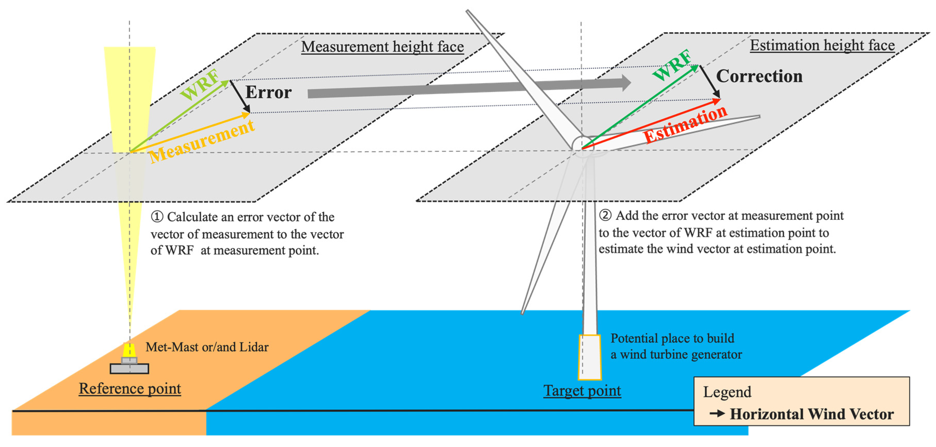
- Offline method: Temporal Correction method (TC)
- (d)
- Offline method: directional extrapolation method (DE)
- (e)
- Direct-application method (DA)
2.3. Evaluation Parameters
2.3.1. General Key Performance Indicators (KPIs)
2.3.2. Wind Speed Difference Between Reference and Target Points
3. Results
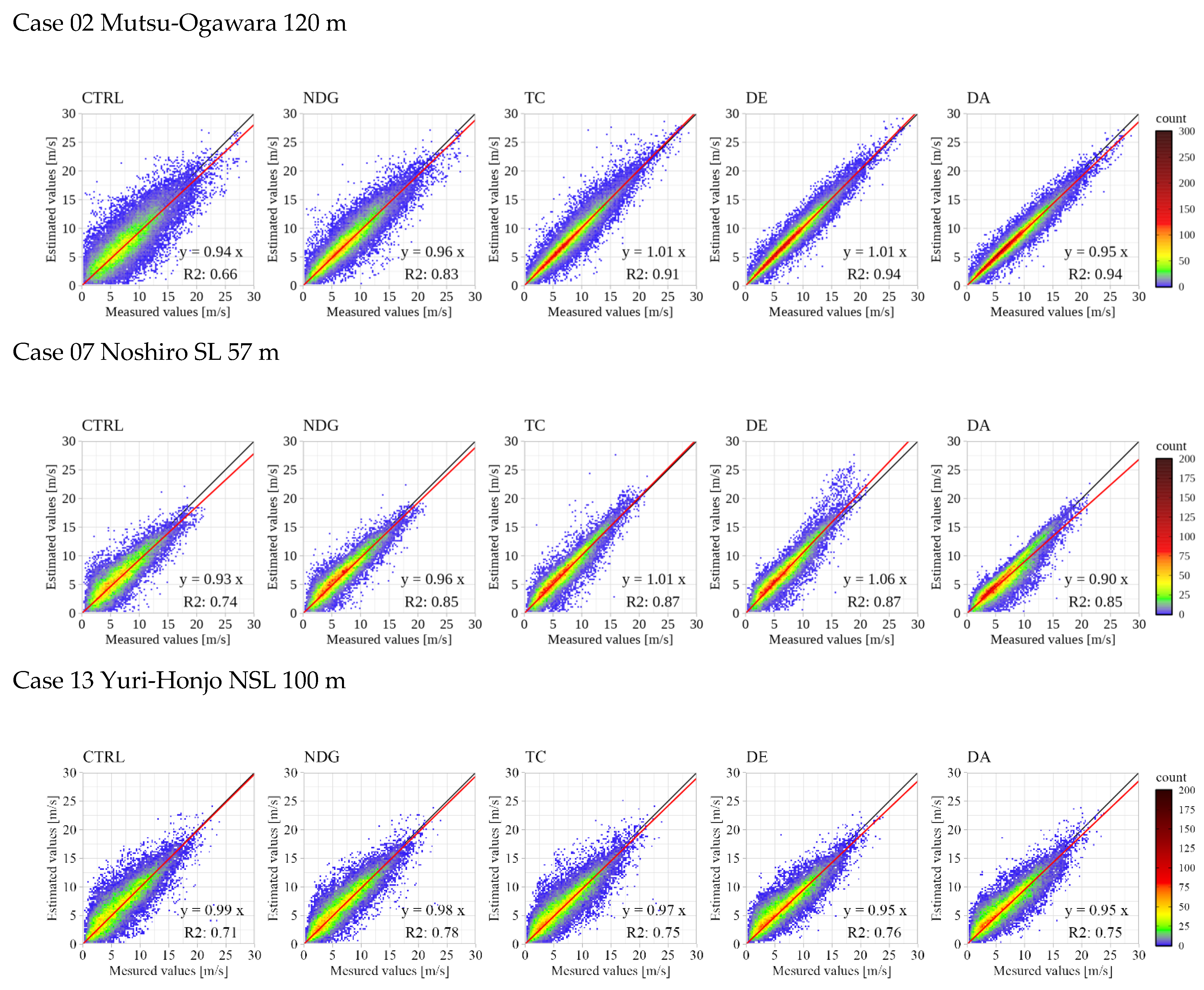
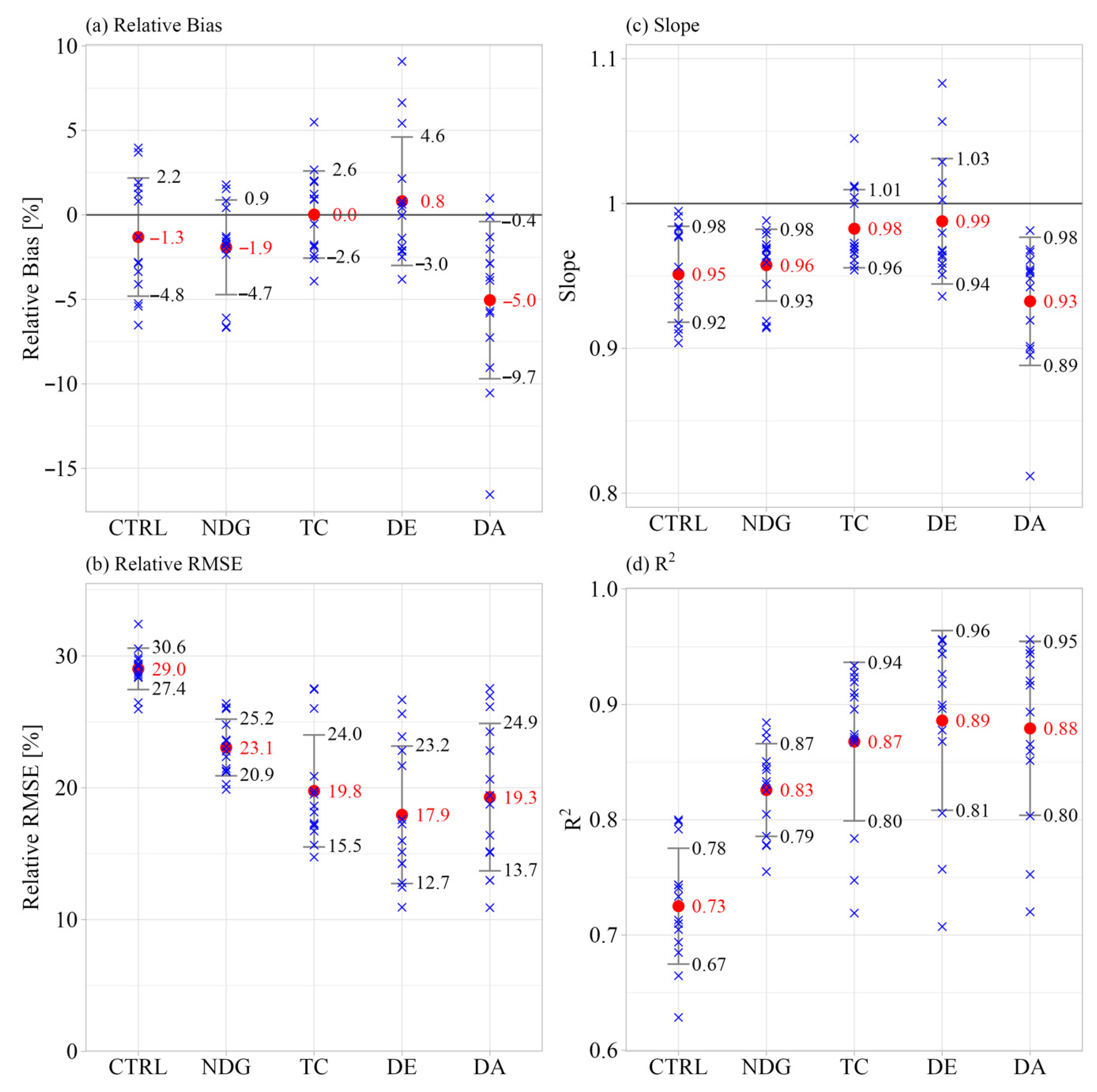
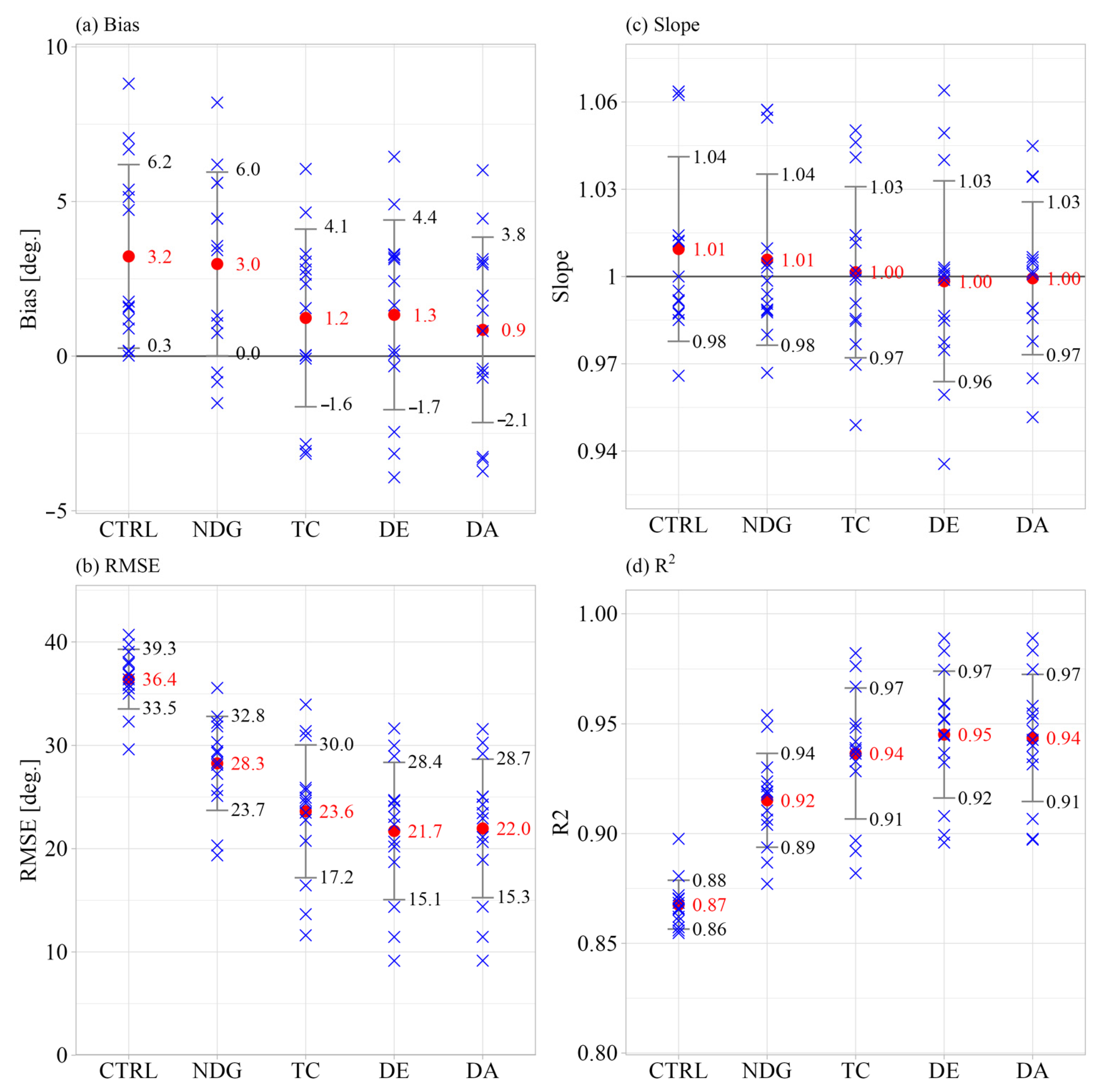
3.1. KPIs of Estimation Time Series by Five Estimation Methods
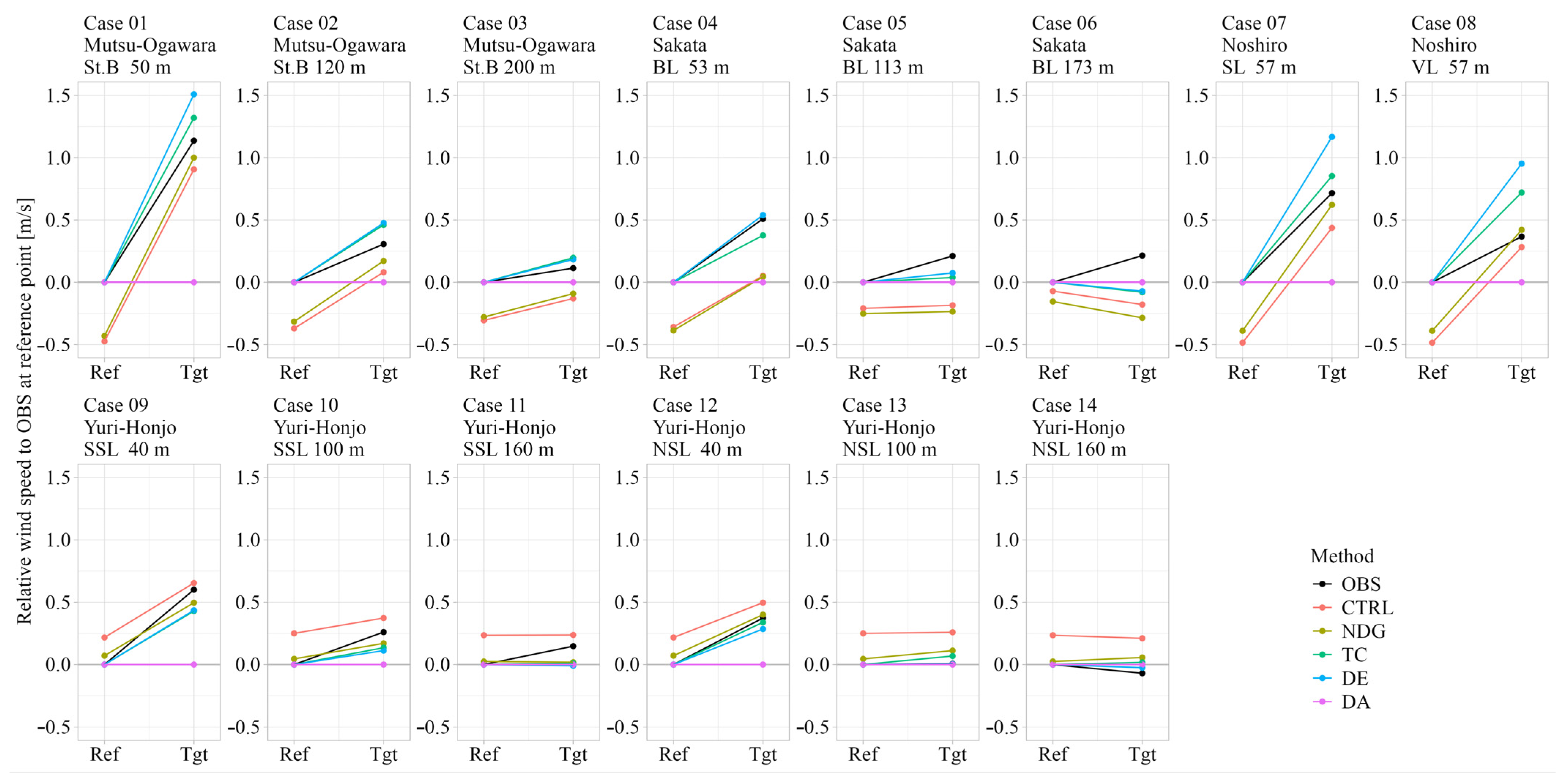
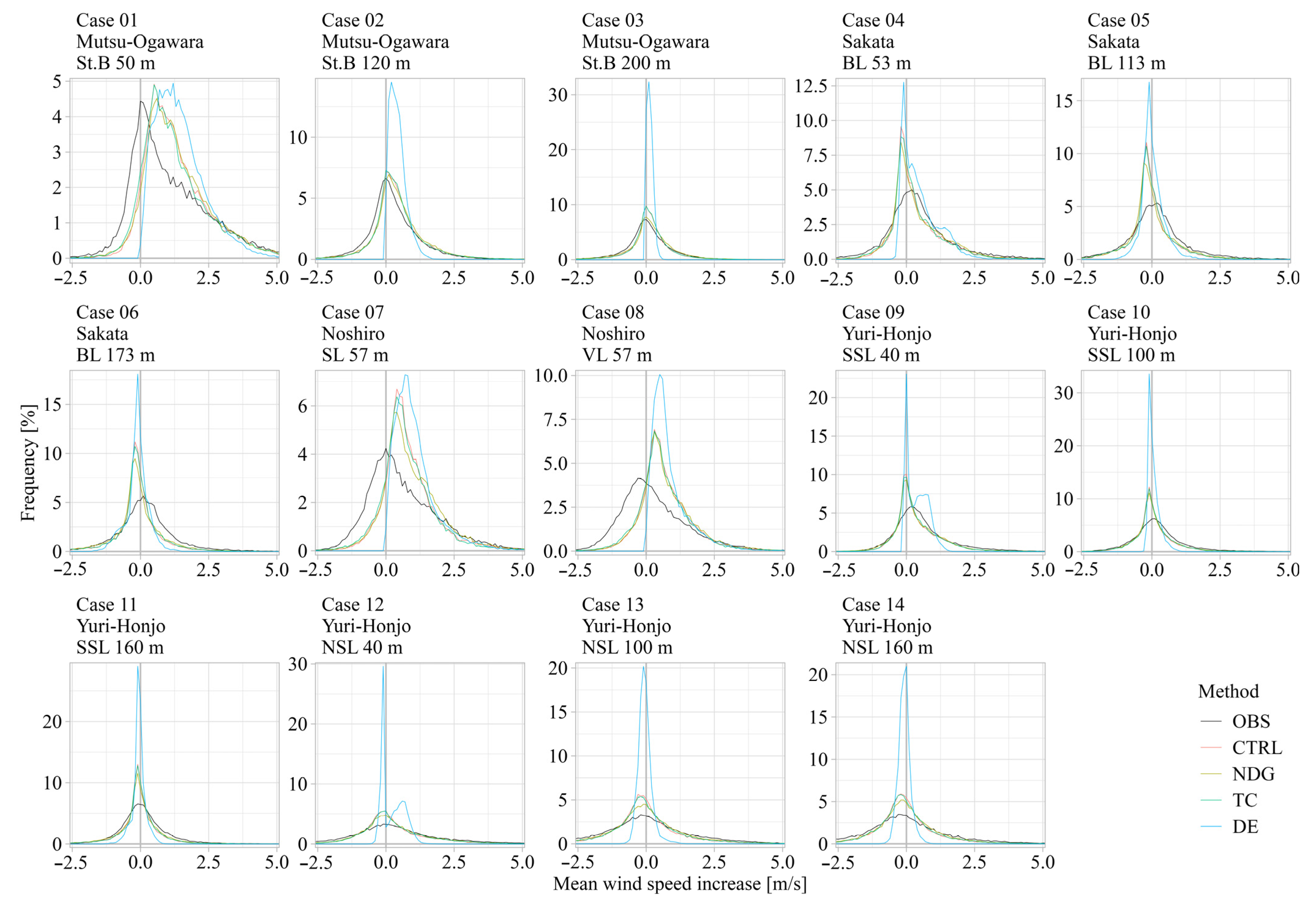
3.2. Accuracy of Wind Speed Difference Between Reference and Target Points
3.3. Evaluation of KPIs That Consider the Characteristics of Each Site
4. Discussion
5. Conclusions
Author Contributions
Funding
Institutional Review Board Statement
Informed Consent Statement
Data Availability Statement
Acknowledgments
Conflicts of Interest
Appendix A
All Statistics Indicators

| Case | Height AMSL [m] | Rel. Bias [%] | Rel. RMSE [%] | Slope | R2 | ||||||||||||||||
|---|---|---|---|---|---|---|---|---|---|---|---|---|---|---|---|---|---|---|---|---|---|
| CTRL | NDG | TC | DE | DA | CTRL | NDG | TC | DE | DA | CTRL | NDG | TC | DE | DA | CTRL | NDG | TC | DE | DA | ||
| Mutsu-Ogawara St. B distance: 1604 m | |||||||||||||||||||||
| 01 | 53 | −3.4 | −2.0 | 2.7 | 5.4 | −16.6 | 32.4 | 24.8 | 19.5 | 17.6 | 27.0 | 0.92 | 0.94 | 1.00 | 1.03 | 0.81 | 0.63 | 0.78 | 0.87 | 0.90 | 0.86 |
| 02 | 113 | −2.9 | −1.7 | 2.0 | 2.1 | −3.9 | 30.5 | 21.3 | 16.7 | 12.8 | 13.0 | 0.94 | 0.96 | 1.01 | 1.01 | 0.95 | 0.66 | 0.83 | 0.91 | 0.94 | 0.94 |
| 03 | 173 | −2.8 | −2.4 | 1.0 | 0.8 | −1.3 | 28.4 | 21.5 | 14.7 | 10.9 | 10.9 | 0.94 | 0.96 | 1.00 | 1.00 | 0.98 | 0.71 | 0.83 | 0.92 | 0.96 | 0.96 |
| Sakata BL distance: 3374 m | |||||||||||||||||||||
| 04 | 50 | −6.5 | −6.6 | −1.9 | 0.4 | −7.3 | 28.6 | 23.1 | 18.6 | 17.3 | 19.4 | 0.90 | 0.91 | 0.97 | 0.98 | 0.92 | 0.79 | 0.87 | 0.91 | 0.92 | 0.92 |
| 05 | 120 | −5.4 | −6.1 | −2.4 | −1.9 | −2.9 | 28.4 | 22.4 | 17.3 | 15.1 | 16.4 | 0.91 | 0.92 | 0.97 | 0.97 | 0.95 | 0.80 | 0.88 | 0.93 | 0.94 | 0.93 |
| 06 | 200 | −5.2 | −6.7 | −3.9 | −3.8 | −2.9 | 28.8 | 23.6 | 17.2 | 14.3 | 15.1 | 0.91 | 0.92 | 0.96 | 0.96 | 0.96 | 0.80 | 0.88 | 0.93 | 0.96 | 0.95 |
| Noshiro SL distance: 4065 m | |||||||||||||||||||||
| 07 | 57 | −4.1 | −1.4 | 2.0 | 6.6 | −10.5 | 26.0 | 19.9 | 19.7 | 21.7 | 22.8 | 0.93 | 0.96 | 1.01 | 1.06 | 0.90 | 0.74 | 0.85 | 0.87 | 0.87 | 0.85 |
| Noshiro VL distance: 4290 m | |||||||||||||||||||||
| 08 | 57 | −1.3 | 0.8 | 5.5 | 9.1 | −5.7 | 26.5 | 20.3 | 20.9 | 22.8 | 20.6 | 0.96 | 0.99 | 1.04 | 1.08 | 0.94 | 0.74 | 0.85 | 0.87 | 0.88 | 0.87 |
| Yuri-Honjo SSL distance: 2115 m | |||||||||||||||||||||
| 09 | 40 | 0.8 | −1.6 | −2.6 | −2.5 | −9.0 | 29.2 | 22.8 | 18.2 | 16.0 | 18.7 | 0.98 | 0.97 | 0.96 | 0.96 | 0.90 | 0.68 | 0.80 | 0.87 | 0.90 | 0.89 |
| 10 | 100 | 1.6 | −1.3 | −1.8 | −2.1 | −3.7 | 29.7 | 21.2 | 17.1 | 14.3 | 15.2 | 0.98 | 0.97 | 0.97 | 0.96 | 0.95 | 0.70 | 0.84 | 0.90 | 0.93 | 0.92 |
| 11 | 160 | 1.2 | −1.8 | −1.9 | −2.2 | −2.0 | 29.4 | 23.6 | 15.7 | 12.5 | 13.0 | 0.98 | 0.97 | 0.97 | 0.97 | 0.97 | 0.73 | 0.83 | 0.92 | 0.95 | 0.94 |
| Yuri-Honjo NSL distance: 11,890 m | |||||||||||||||||||||
| 12 | 40 | 1.9 | 0.4 | −0.5 | −1.4 | −5.8 | 29.4 | 26.1 | 27.5 | 26.7 | 27.5 | 0.98 | 0.97 | 0.95 | 0.94 | 0.90 | 0.69 | 0.75 | 0.72 | 0.71 | 0.72 |
| 13 | 100 | 3.7 | 1.5 | 0.9 | 0.0 | −0.1 | 29.9 | 26.0 | 27.5 | 25.6 | 26.1 | 0.99 | 0.98 | 0.97 | 0.95 | 0.95 | 0.71 | 0.78 | 0.75 | 0.76 | 0.75 |
| 14 | 160 | 4.0 | 1.8 | 1.2 | 0.6 | 1.0 | 29.2 | 26.4 | 26.0 | 23.9 | 24.3 | 0.99 | 0.98 | 0.97 | 0.96 | 0.97 | 0.74 | 0.79 | 0.78 | 0.81 | 0.80 |
| Mean | −1.3 | −1.9 | 0.0 | 0.8 | −5.0 | 29.0 | 23.1 | 19.8 | 17.9 | 19.3 | 0.95 | 0.96 | 0.98 | 0.99 | 0.93 | 0.73 | 0.83 | 0.87 | 0.89 | 0.88 | |
| Std. Dev. | 3.5 | 2.8 | 2.6 | 3.8 | 4.6 | 1.6 | 2.1 | 4.2 | 5.2 | 5.6 | 0.03 | 0.02 | 0.03 | 0.04 | 0.04 | 0.05 | 0.04 | 0.07 | 0.08 | 0.08 | |
| Case | Height AMSL [m] | Bias [deg.] | RMSE [deg.] | Slope | Intercept | R2 | ||||||||||||||||||||
|---|---|---|---|---|---|---|---|---|---|---|---|---|---|---|---|---|---|---|---|---|---|---|---|---|---|---|
| CTRL | NDG | TC | DE | DA | CTRL | NDG | TC | DE | DA | CTRL | NDG | TC | DE | DA | CTRL | NDG | TC | DE | DA | CTRL | NDG | TC | DE | DA | ||
| Mutsu-Ogawara St. B distance: 1604 m | ||||||||||||||||||||||||||
| 01 | 53 | 0.9 | 0.7 | −0.1 | −0.1 | −0.7 | 35.0 | 25.7 | 16.4 | 14.4 | 14.4 | 0.99 | 0.99 | 1.00 | 1.00 | 1.01 | 4.0 | 2.7 | −0.5 | −1.0 | −2.1 | 0.86 | 0.92 | 0.97 | 0.97 | 0.97 |
| 02 | 113 | 1.2 | 1.1 | 0.0 | 0.0 | −0.5 | 32.3 | 19.4 | 13.7 | 11.5 | 11.5 | 1.00 | 1.00 | 1.00 | 1.00 | 1.00 | 1.2 | 0.4 | 0.3 | 0.1 | −1.5 | 0.88 | 0.95 | 0.98 | 0.98 | 0.98 |
| 03 | 173 | 1.8 | 1.3 | 0.0 | 0.0 | −0.4 | 29.6 | 20.3 | 11.6 | 9.1 | 9.2 | 1.01 | 1.01 | 1.00 | 1.00 | 1.00 | −1.2 | −0.7 | 0.0 | 0.3 | −0.7 | 0.90 | 0.95 | 0.98 | 0.99 | 0.99 |
| Sakata BL distance: 3374 m | ||||||||||||||||||||||||||
| 04 | 50 | 0.2 | −0.5 | −3.2 | −3.2 | −3.7 | 40.7 | 31.8 | 25.9 | 24.7 | 25.0 | 1.06 | 1.06 | 1.05 | 1.06 | 1.04 | −12.7 | −12.4 | −13.5 | −17.1 | −13.0 | 0.86 | 0.91 | 0.94 | 0.95 | 0.94 |
| 05 | 120 | 0.0 | −1.5 | −3.1 | −3.1 | −3.3 | 39.8 | 29.5 | 24.4 | 22.3 | 22.9 | 1.06 | 1.05 | 1.05 | 1.05 | 1.03 | −13.4 | −13.0 | −12.8 | −13.5 | −10.5 | 0.86 | 0.92 | 0.94 | 0.95 | 0.95 |
| 06 | 200 | 0.2 | −0.8 | −2.8 | −2.8 | −3.3 | 38.1 | 29.3 | 22.8 | 20.2 | 21.1 | 1.06 | 1.06 | 1.04 | 1.04 | 1.03 | −13.4 | −13.1 | −11.6 | −11.0 | −10.6 | 0.87 | 0.92 | 0.95 | 0.96 | 0.95 |
| Noshiro SL distance: 4065 m | ||||||||||||||||||||||||||
| 07 | 57 | 1.6 | 3.4 | 2.8 | 2.8 | 3.0 | 36.4 | 27.2 | 25.7 | 24.6 | 25.1 | 1.01 | 1.00 | 1.01 | 1.00 | 1.01 | −0.9 | 2.5 | −0.1 | 2.7 | 1.8 | 0.87 | 0.92 | 0.93 | 0.94 | 0.93 |
| Noshiro VL distance: 4290 m | ||||||||||||||||||||||||||
| 08 | 57 | 1.6 | 3.6 | 2.6 | 2.6 | 3.0 | 36.8 | 28.1 | 24.7 | 23.1 | 23.4 | 1.01 | 1.00 | 1.01 | 1.00 | 1.00 | −0.8 | 3.8 | 0.3 | 3.1 | 2.9 | 0.87 | 0.92 | 0.94 | 0.94 | 0.94 |
| Yuri-Honjo SSL distance: 2115 m | ||||||||||||||||||||||||||
| 09 | 40 | 5.4 | 5.6 | 3.1 | 3.1 | 2.0 | 37.9 | 30.3 | 23.5 | 20.7 | 20.6 | 0.99 | 0.98 | 0.98 | 0.97 | 0.99 | 7.9 | 9.5 | 7.6 | 8.1 | 4.8 | 0.86 | 0.90 | 0.94 | 0.95 | 0.95 |
| 10 | 100 | 4.7 | 4.5 | 2.3 | 2.4 | 1.5 | 35.9 | 25.1 | 20.8 | 18.7 | 18.9 | 0.99 | 0.99 | 0.98 | 0.98 | 0.99 | 6.4 | 6.8 | 5.4 | 5.5 | 3.6 | 0.87 | 0.93 | 0.95 | 0.96 | 0.96 |
| 11 | 160 | 5.1 | 4.4 | 1.6 | 1.6 | 0.8 | 35.5 | 28.4 | 24.9 | 24.1 | 24.3 | 0.99 | 0.99 | 0.99 | 0.99 | 0.99 | 7.6 | 6.9 | 3.4 | 4.4 | 3.0 | 0.87 | 0.91 | 0.93 | 0.93 | 0.93 |
| Yuri-Honjo NSL distance: 11,890 m | ||||||||||||||||||||||||||
| 12 | 40 | 8.8 | 8.2 | 6.1 | 6.4 | 6.0 | 39.1 | 35.6 | 34.0 | 31.6 | 31.6 | 0.97 | 0.97 | 0.95 | 0.94 | 0.95 | 15.4 | 14.6 | 15.9 | 18.9 | 15.3 | 0.85 | 0.88 | 0.88 | 0.90 | 0.90 |
| 13 | 100 | 7.1 | 6.2 | 4.6 | 4.9 | 4.4 | 36.9 | 32.2 | 30.9 | 29.0 | 29.2 | 0.99 | 0.99 | 0.97 | 0.96 | 0.97 | 8.7 | 8.4 | 10.6 | 12.9 | 11.4 | 0.87 | 0.89 | 0.90 | 0.91 | 0.91 |
| 14 | 160 | 6.7 | 5.6 | 3.3 | 3.3 | 3.1 | 35.9 | 32.8 | 31.4 | 30.0 | 30.3 | 1.00 | 0.99 | 0.99 | 0.98 | 0.98 | 7.7 | 6.8 | 6.2 | 7.8 | 7.6 | 0.87 | 0.89 | 0.89 | 0.90 | 0.90 |
| Mean | 3.2 | 3.0 | 1.2 | 1.3 | 0.9 | 36.4 | 28.3 | 23.6 | 21.7 | 22.0 | 1.01 | 1.01 | 1.00 | 1.00 | 1.00 | 1.2 | 1.7 | 0.8 | 1.5 | 0.9 | 0.87 | 0.92 | 0.94 | 0.95 | 0.94 | |
| Std. Dev. | 3.0 | 3.0 | 2.9 | 3.1 | 3.0 | 2.9 | 4.5 | 6.4 | 6.6 | 6.7 | 0.03 | 0.03 | 0.03 | 0.03 | 0.03 | 9.0 | 8.8 | 8.7 | 9.9 | 8.2 | 0.01 | 0.02 | 0.03 | 0.03 | 0.03 | |
| Case | Height AMSL [m] | Rel. Bias [%] | Rel. RMSE [%] | Slope | R2 | ||||
|---|---|---|---|---|---|---|---|---|---|
| CTRL | NDG | CTRL | NDG | CTRL | NDG | CTRL | NDG | ||
| Mutsu-Ogawara St. A | |||||||||
| 01 | 50 | −5.5 | −6.0 | 29.6 | 22.5 | 0.92 | 0.93 | 0.79 | 0.88 |
| 02 | 120 | −2.9 | −3.5 | 27.6 | 18.6 | 0.94 | 0.95 | 0.80 | 0.91 |
| 03 | 200 | −1.0 | −2.1 | 27.1 | 19.6 | 0.95 | 0.96 | 0.81 | 0.90 |
| Sakata LL | |||||||||
| 04 | 53 | −8.3 | −7.5 | 32.6 | 25.1 | 0.88 | 0.90 | 0.63 | 0.78 |
| 05 | 113 | −4.9 | −4.2 | 30.2 | 19.9 | 0.92 | 0.94 | 0.66 | 0.85 |
| 06 | 173 | −3.6 | −3.2 | 28.0 | 21.7 | 0.94 | 0.95 | 0.71 | 0.82 |
| Noshiro CMT | |||||||||
| 07, 08 | 57 | −8.0 | −6.4 | 29.0 | 19.8 | 0.89 | 0.92 | 0.74 | 0.89 |
| Yuri-Honjo SVL | |||||||||
| 09, 12 | 40 | 3.6 | 1.2 | 31.3 | 23.6 | 1.00 | 1.00 | 0.66 | 0.80 |
| 10, 13 | 100 | 3.7 | 0.7 | 30.5 | 20.1 | 1.00 | 1.00 | 0.68 | 0.86 |
| 11, 14 | 160 | 3.3 | 0.3 | 29.7 | 22.2 | 1.00 | 0.99 | 0.72 | 0.84 |
| Mean | −2.4 | −3.1 | 29.6 | 21.3 | 0.94 | 0.95 | 0.72 | 0.85 | |
| Std. Dev. | 4.6 | 3.1 | 1.7 | 2.1 | 0.05 | 0.03 | 0.06 | 0.04 | |
| Case | Height AMSL [m] | Bias [deg.] | RMSE [deg.] | Slope | Intercept | R2 | |||||
|---|---|---|---|---|---|---|---|---|---|---|---|
| CTRL | NDG | CTRL | NDG | CTRL | NDG | CTRL | NDG | CTRL | NDG | ||
| Mutsu-Ogawara St. A | |||||||||||
| 01 | 50 | 3.0 | 2.2 | 41.0 | 31.6 | 1.00 | 1.00 | 3.5 | 2.7 | 0.85 | 0.90 |
| 02 | 120 | 2.9 | 1.4 | 38.8 | 24.9 | 1.01 | 1.01 | 0.4 | −0.3 | 0.86 | 0.94 |
| 03 | 200 | 3.1 | 1.6 | 36.7 | 26.4 | 1.01 | 1.01 | 0.1 | −0.7 | 0.88 | 0.93 |
| Sakata LL | |||||||||||
| 04 | 53 | 1.3 | 1.4 | 36.0 | 27.6 | 0.98 | 0.98 | 5.8 | 5.9 | 0.85 | 0.91 |
| 05 | 113 | 1.3 | 1.0 | 33.4 | 19.7 | 1.00 | 1.00 | 1.1 | 1.3 | 0.88 | 0.95 |
| 06 | 173 | 1.7 | 1.5 | 29.9 | 23.4 | 1.01 | 1.01 | −0.8 | 0.5 | 0.90 | 0.93 |
| Noshiro CMT | |||||||||||
| 07, 08 | 57 | −1.3 | 0.1 | 39.7 | 27.2 | 0.99 | 0.99 | 0.0 | 1.9 | 0.85 | 0.92 |
| Yuri-Honjo SVL | |||||||||||
| 09, 12 | 40 | 2.7 | 2.7 | 38.7 | 31.0 | 1.00 | 0.99 | 2.1 | 4.5 | 0.85 | 0.90 |
| 10, 13 | 100 | 2.7 | 2.0 | 36.5 | 25.2 | 1.00 | 1.00 | 1.9 | 2.0 | 0.86 | 0.93 |
| 11, 14 | 160 | 3.6 | 2.9 | 38.0 | 30.3 | 1.00 | 1.00 | 4.0 | 3.8 | 0.85 | 0.90 |
| Mean | 2.1 | 1.7 | 36.9 | 26.7 | 36.9 | 26.7 | 1.8 | 2.2 | 0.86 | 0.92 | |
| Std. Dev. | 1.4 | 0.8 | 3.2 | 3.7 | 3.2 | 3.7 | 2.1 | 2.1 | 0.02 | 0.02 | |
References
- MEASNET. Evaluation of Site-Specific Wind Conditions; Version 3; MEASNET: Madrid, Spain, 2022; p. 64. [Google Scholar]
- Climate Integrate. Offshore Wind in Japan: Policy Agenda and Prospects; Climate Integrate: Tokyo, Japan, 2024; Available online: https://climateintegrate.org/wp-content/uploads/2024/04/Offshore-Wind-in-Japan-EN.pdf (accessed on 27 June 2025).
- Troen, I.; Petersen, E.L. European Wind Atlas; Risø National Laboratory: Roskilde, Denmark, 1989. [Google Scholar]
- Dayal, A.; Prasad, A.; Deo, R.C. Wind Resource Assessment and Energy Potential of Selected Locations in Fiji. Renew. Energy 2021, 172, 292–307. [Google Scholar] [CrossRef]
- Al-Deen, S.; Yamaguchi, A.; Ishihara, T. A Physical Approach to Wind Speed Prediction for Wind Energy Forecasting. In Proceedings of the Fourth International Symposium on Computational Wind Engineering, Yokohama, Japan, 16–19 July 2006; pp. 349–352. [Google Scholar]
- Konagaya, M.; Ohsawa, T.; Mito, T.; Misaki, T.; Maruo, T.; Baba, Y. Estimation of nearshore wind conditions using onshore observation data with computational fluid dynamic and mesoscale models. Resources 2022, 11, 100. [Google Scholar] [CrossRef]
- Uchida, T. Computational Fluid Dynamics Approach to Predict the Actual Wind Speed over Complex Terrain. Energies 2018, 11, 1694. [Google Scholar] [CrossRef]
- Stull, R.B. An Introduction to Boundary Layer Meteorology, 1st ed.; Springer: Dordrecht, The Netherlands, 1988; ISBN 978-90-277-2768-8. [Google Scholar]
- De Tomasi, F.; Miglietta, M.M.; Perrone, R. The growth of the planetary boundary layer at a coastal site: A case study. Bound.-Layer Meteorol. 2011, 139, 521–541. [Google Scholar] [CrossRef]
- Floors, R.; Batchvarova, E.; Gryning, S.-E.; Peña, A. Atmospheric boundary layer wind profile at a flat coastal site—Wind speed lidar measurements and mesoscale modeling results. J. Appl. Meteorol. Climatol. 2011, 50, 1694–1705. [Google Scholar] [CrossRef]
- Dörenkämper, M.; Optis, M.; Monahan, A.; Steinfeld, G. On the offshore advection of boundary-layer structures and the influence on offshore wind conditions. Bound.-Layer Meteorol. 2015, 155, 459–482. [Google Scholar] [CrossRef]
- Lo Feudo, T.; Calidonna, C.R.; Avolio, E.; Sempreviva, A.M. Study of the Vertical Structure of the Coastal Boundary Layer Integrating Surface Measurements and Ground-Based Remote Sensing. Sensors 2020, 20, 6516. [Google Scholar] [CrossRef]
- Milovac, J.; Ingwersen, J.; Warrach-Sagi, K. Multi-nested WRF simulations for studying planetary boundary layer height and structure across the coastal zone. Tellus A 2020, 72, e17674. [Google Scholar] [CrossRef]
- Kikuchi, Y.; Fukushima, M.; Ishihara, T. Assessment of a Coastal Offshore Wind Climate by Means of Mesoscale Model Simulations Considering High-Resolution Land Use and Sea Surface Temperature Data Sets. Atmosphere 2020, 11, 379. [Google Scholar] [CrossRef]
- Konagaya, M.; Ohsawa, T.; Itoshima, Y.; Kambayashi, M.; Leonard, E.; Tromeur, E.; Misaki, T.; Shintaku, E.; Araki, R.; Hamada, K. Estimation of Wind Conditions in the Offshore Direction Using Multiple Numerical Models and In Situ Observations. Energies 2025, 18, 3000. [Google Scholar] [CrossRef]
- Misaki, T.; Ohsawa, T.; Konagaya, M.; Shimada, S.; Takeyama, Y.; Nakamura, S. Accuracy Comparison of Coastal Wind Speeds between WRF Simulations Using Different Input Datasets in Japan. Energies 2019, 12, 2754. [Google Scholar] [CrossRef]
- Skamarock, W.C.; Klemp, J.B.; Duhia, J.; Gill, D.O.; Liu, Z.; Berner, J.; Wang, W.; Powers, J.G.; Duda, M.G.; Barker, D.M.; et al. A Description of the Advanced Research WRF Model; Version 4; NCAR Technical Notes; National Center for Atmospheric Research: Boulder, CO, USA, 2019. [Google Scholar]
- Reen, B.P. A Brief Guide to Observation Nudging in WRF; Battlefield Environment Division, Army Research Laboratory: Adelphi, MD, USA, 2016; Available online: https://raw.githubusercontent.com/wrf-model/OBSGRID/master/ObsNudgingGuide.pdf (accessed on 29 June 2025).
- Gryning, S.-E.; Batchvarova, E.; Floors, R. A study on the effect of nudging on long-term boundary layer profiles of Wind and Weibull distribution parameters in a rural coastal area. J. Appl. Meteorol. Climatol. 2013, 52, 1201–1207. [Google Scholar] [CrossRef]
- Mylonas, M.P.; Barbouchi, S.; Herrmann, H.; Nastos, P.T. Sensitivity analysis of observational nudging methodology to reduce error in wind resource assessment (WRA) in the North Sea. Renew. Energ. 2018, 120, 446–456. [Google Scholar] [CrossRef]
- Désert, T.; Knapp, G.; Aubrun, S. Quantification and correction of wave-induced turbulence intensity bias for a floating LIDAR system. Remote Sens. 2021, 13, 2973. [Google Scholar] [CrossRef]
- Kotake, N.; Kameyama, S.; Kajiyama, Y.; Enjo, M. Performance analysis of Mitsubishi Electric’s wind lidar in the measurement campaign at European test sites. In Proceedings of the WindEurope Summit, Hamburg, Germany, 27–29 September 2016. [Google Scholar]
- Branlard, E.; Pedersen, A.T.; Mann, J.; Angelou, N.; Fischer, A.; Mikkelsen, T.; Harris, M.; Slinger, C.; Montes, B.F. Retrieving wind statistics from average spectrum of continuous-wave lidar. Atmos. Meas. Tech. 2013, 6, 1673–1683. [Google Scholar] [CrossRef]
- Peña, A.; Mann, J. Turbulence measurements with Dual-Doppler scanning lidars. Remote Sens. 2019, 11, 2444. [Google Scholar] [CrossRef]
- Simon, E.; Courtny, M. A Comparison of Sector-Scan and Dual Doppler Wind Measurements at Høvsøre Test Station—One Lidar or Two? DTU Wind Energy Report E-0112; DTU Library: Roskilde, Denmark, 2016. [Google Scholar]
- Misaki, T. A Study on Improving the Accuracy of Coastal Wind Speeds Simulated by Mesoscale Model. Ph.D. Thesis, Kobe University, Kobe, Japan, 2020; p. 78. [Google Scholar]
- Stauffer, D.R.; Seaman, N.L. Use of Four-Dimensional Data Assimilation in a Limited-Area Mesoscale Model. Part I: Experiments with Synoptic-Scale Data. Mon. Weather Rev. 1990, 118, 1250–1277. [Google Scholar] [CrossRef]
- Qian, G.-W.; Ishihara, T. A novel probabilistic power curve model to predict the power production and its uncertainty for a wind farm over complex terrain. Energy. 2022, 261, 125171. [Google Scholar] [CrossRef]
- Misu, Y.; Ishihara, T. Prediction of frequency distribution of strong crosswind in a control section for train operations by using onsite measurement and numerical simulation. J. Wind Eng. Ind. Aerodyn. 2018, 174, 69–79. [Google Scholar] [CrossRef]
- Chai, T.; Draxler, R.R. Root mean square error (RMSE) or mean absolute error (MAE)?—Arguments against avoiding RMSE in the literature. Geosci. Model Dev. 2014, 7, 1247–1250. [Google Scholar] [CrossRef]
- DNV GL; Frazer-Nash Consultancy; Multiversum Consulting; Fraunhofer IWES. Carbon Trust Offshore Wind Accelerator Road Map for the Commercial Acceptance of Floating LiDAR Technology Version 2.0; Carbon Trust: London, UK, 2018; p. 149. [Google Scholar]
- Kvålseth, T.O. Cautionary note about R 2. Am. Stat. 1985, 39, 279–285. [Google Scholar] [CrossRef]

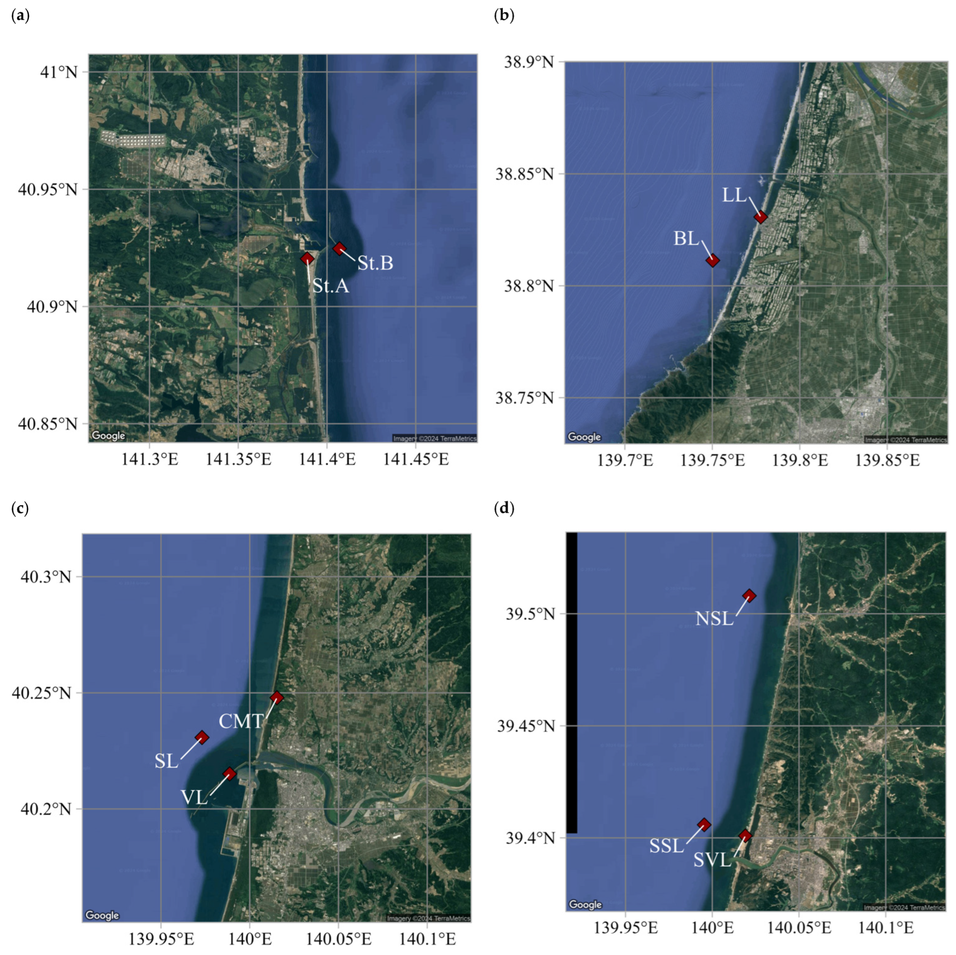


| Site | Point | Method | Scan | Equipment | Specification and Settings of Scan | Height Used for Analysis (from AMSL) [m] | Installation Situation |
|---|---|---|---|---|---|---|---|
| Mutsu-Ogawara | St. A | VL | DBS | Windcube V2.1 | SR: 1 Hz (0.8 s/pulses) 4 inclined beams at 28° and 1 vertical beam Measured: 12 heights | 50, 66, 87, 107, 127, 147, 167, 187, 207 | On land |
| St. B | VL | DBS | Windcube V2.1 | Same as above | 50, 120, 200 | On breakwater | |
| Sakata | LL | VL | DBS | DIABREZZA | Measured: 20 heights 4 inclined beams at 30° and 1 vertical beam | 51.5, 71.5, …, 211.5 | On land |
| BL | VL | DBS | DIABREZZA | Same as above | 53, 113, 173 | On buoy | |
| Noshiro | CMT | Cup and Vane | - | - | SR: 1 Hz Measured: 1 height | 57.0 | Installed meteorological mast on land |
| SL | DSL | RHI | Windcube 200S×2 | SR: 1 Hz Included Angle: 42.3° Gate Length: 50 m Measured: 3 heights | 28, 115 | On land, but measuring offshore point | |
| VL | VL | VAD (CW) | ZX LiDAR 300M | SR: 1 Hz Measured: 3 heights 50 LoS/1 s at 30° Measured: 8 heights | 26, 113 | On breakwater | |
| Yuri-Honjo | SVL | VL | VAD (CW) | ZX LiDAR 300M | Same as above Measured: 5 heights | 40, 100, 160 | On land |
| SSL | SSL | PPI | StreamLine XR | SR: 1 Hz Sector size: 60°, consisting of 5 LoS Gate Length: 90 m Measured: 3 heights | 40, 100, 160 | On land, but measuring offshore point | |
| NSL | SSL | PPI | StreamLine XR | Same as above | 40, 100, 160 | On land, but measuring offshore point |
| Case | Site | Reference Point | Target Point | Height at Reference and Target Point [m AMSL] | Distance Between Reference and Target Point [m] | Distance Between Shoreline and Target Point [m] | # of Sample |
|---|---|---|---|---|---|---|---|
| 01 | Mutsu-Ogawara | St. A * | St. B | 50 | 1604 | 1040 | 45,157 |
| 02 | 120 | ||||||
| 03 | 200 | ||||||
| 04 | Sakata | LL * | BL | 53 | 3374 | 1380 | 18,119 |
| 05 | 113 | ||||||
| 06 | 173 | ||||||
| 07 | Noshiro | CMT | SL * | 57 | 4065 | 2750 | 28,098 |
| 08 | VL * | 57 | 4290 | 520 | |||
| 09 | Yuri-Honjo | SVL | SSL | 40 | 2115 | 1750 | 29,955 |
| 10 | 100 | ||||||
| 11 | 160 | ||||||
| 12 | NSL | 40 | 11,890 | 2040 | |||
| 13 | 100 | ||||||
| 14 | 160 |
| Abbreviation | Method | Material | Schematic | ||
|---|---|---|---|---|---|
| Measurement | Model Results | ||||
| CTRL | WRF control simulation without on-site measurement data | ✓ | 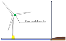 | ||
| NDG | Online method | Observation nudging | ✓ | ✓ | 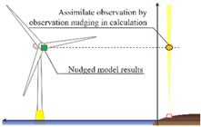 |
| TC | Offline method | Temporal correction method | ✓ | ✓ |  |
| DE | Directional extrapolation method | ✓ | ✓ | ||
| DA | Directly Apply a time series at reference point | ✓ |  | ||
| Model Version | WRF (ARW: Advanced Research WRF) V3.8.1 (Noshiro, Yuri-Honjo)/4.1.2(Sakata, Mutsu-Ogawara) | |
|---|---|---|
| Input data | Met | JMA-LFM (1 hourly, 0.02° × 0.025°) |
| Soil | NCEP FNL (National Centers for Environmental Prediction Final Operational Global Analysis) (6 hourly, 1° × 1°) | |
| SST | Met Office OSTIA (Daily, 0.05° × 0.05°) | |
| Terrain data | Elevation | METI (Ministry of Economy, Trade and Industry (Japan)), NASA (National Aeronautics and Space Administration), ASTER-GDEM (Advanced Spaceborne Thermal Emission and Reflection Radiometer Global Digital Elevation Model) |
| Land use | MEIT, MLNI (Ministry of Land, Infrastructure, Transport and Tourism (Japan)) land use subdivision mesh | |
| Roughness Table | Based on JMA but Mixed Forest (3.0 m by JMA) is 2.0 m in only Noshiro and Yuri-Honjo | |
| Grid spacing | d01 | 2.5 km |
| d02 | 0.5 km | |
| d03 | 0.1 km | |
| Vertical levels | 40 layers (Surface to 100 hPa) | |
| Physics options | Shortwave | Dudhia scheme |
| Longwave | Rapid Radiative Transfer Model scheme | |
| Microphysics | Ferrier (new Eta) scheme | |
| Planetary Boundary Layer | Mellor-Yamada-Janic (Eta operational) scheme | |
| Surface layer | Monin-Obukhov (Janic Eta) scheme | |
| Land surface | Noah Land Surface Model scheme | |
| Cumulus Parameterization | Kain-Fritsch (new Eta) scheme (only d01) | |
| FDDA | d01 | Enabled (u, v, θ, q) |
| d02, d03 | Enabled (u, v, θ, q) above the thirteen layers (about 2 km) | |
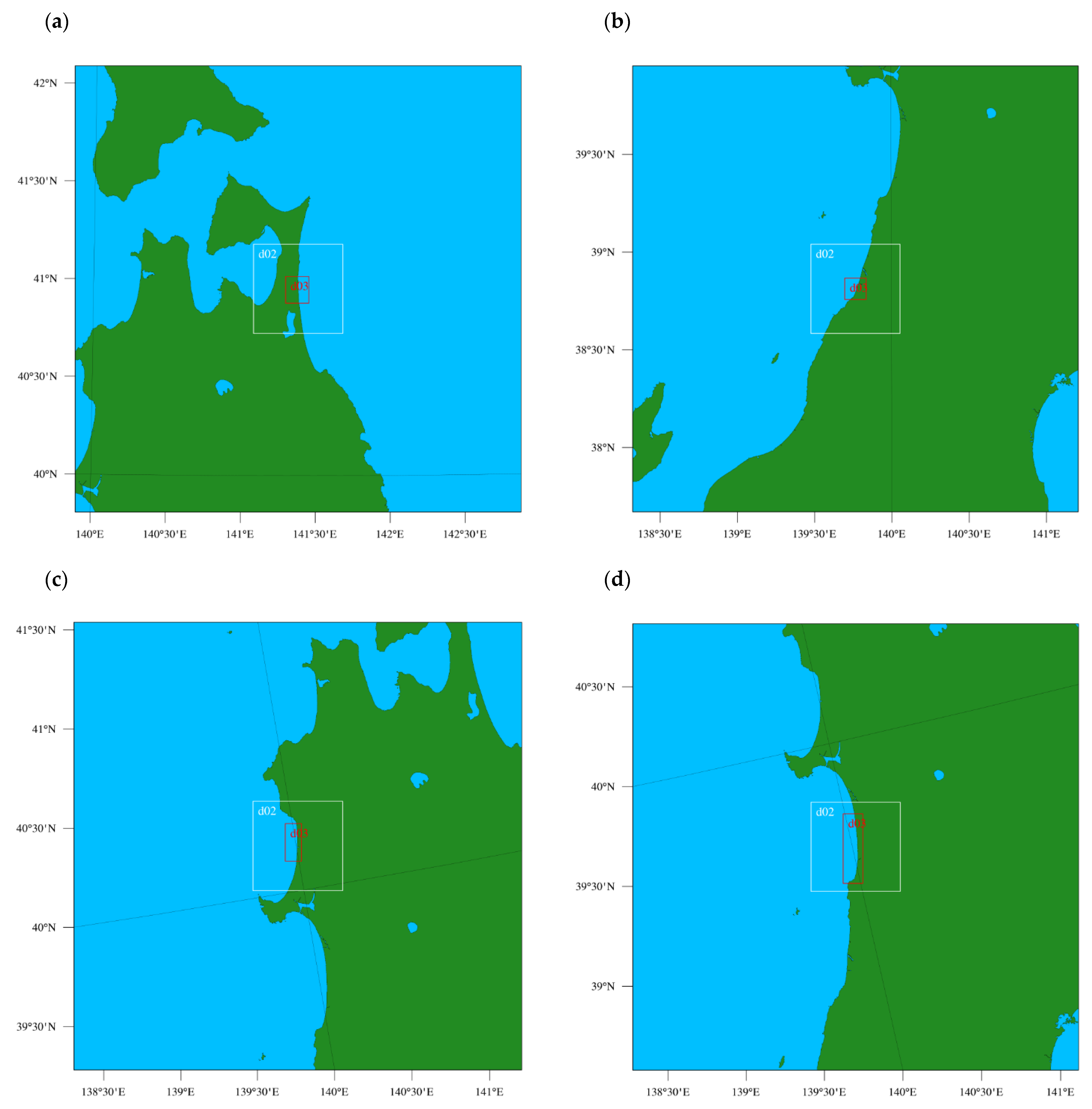
| Site | Period (Not Including the Spin-Up Period) | Grid | |||
|---|---|---|---|---|---|
| d01 | d02 | d03 | |||
| Mutsu-Ogawara | 1 January 2021–31 December 2021 | (1 year) | 100 × 100 | 100 × 100 | 130 × 150 |
| Sakata | 1 July 2018–31 December 2018 | (6 months) | 100 × 100 | 100 × 100 | 120 × 120 |
| Noshiro | 1 August 2020–31 July 2021 | (1 year) | 100 × 100 | 100 × 100 | 90 × 210 |
| Yuri-Honjo | 1 February 2020–31 January 2021 | (1 year) | 100 × 100 | 100 × 100 | 110 × 390 |
| Variable | Setting |
|---|---|
| Valid domain | d03 |
| Input (Reference) data | u- and v-components converted from 10 min horizontal mean wind speed and direction |
| Nudging coefficient | 1.2 × 10⁻³ |
| Horizontal radius of influence | 20 km |
| Half-period time window | 6 min 40 s |
| Case | Site | Reference Point (Its Height [m AMSL]) | Vertical Radius of Influence [m] (Convert Sigma Levels Grid into Meter) |
|---|---|---|---|
| 01–03 | Mutsu-Ogawara | St. A (50, 66, 87, 107, …, 207) | About 20 |
| 04–06 | Sakata | LL (51.5, 71.5, …, 211.5) | About 20 |
| 07–08 | Noshiro | CMT (57) | About 60 |
| 09–14 | Yuri-Honjo | SVL (40, 100, 160) | About 60 |
| Diff. | Ratio | |||||
|---|---|---|---|---|---|---|
| Method | Slope | Intercept | R | Slope | Intercept | R |
| CTRL | 1.22 | −0.08 | 0.90 | 1.32 | −0.34 | 0.91 |
| NDG | 1.25 | −0.06 | 0.88 | 1.35 | −0.36 | 0.90 |
| TC | 1.12 | −0.04 | 0.89 | 1.13 | −0.14 | 0.92 |
| DE | 1.38 | −0.08 | 0.89 | 1.38 | −0.39 | 0.90 |
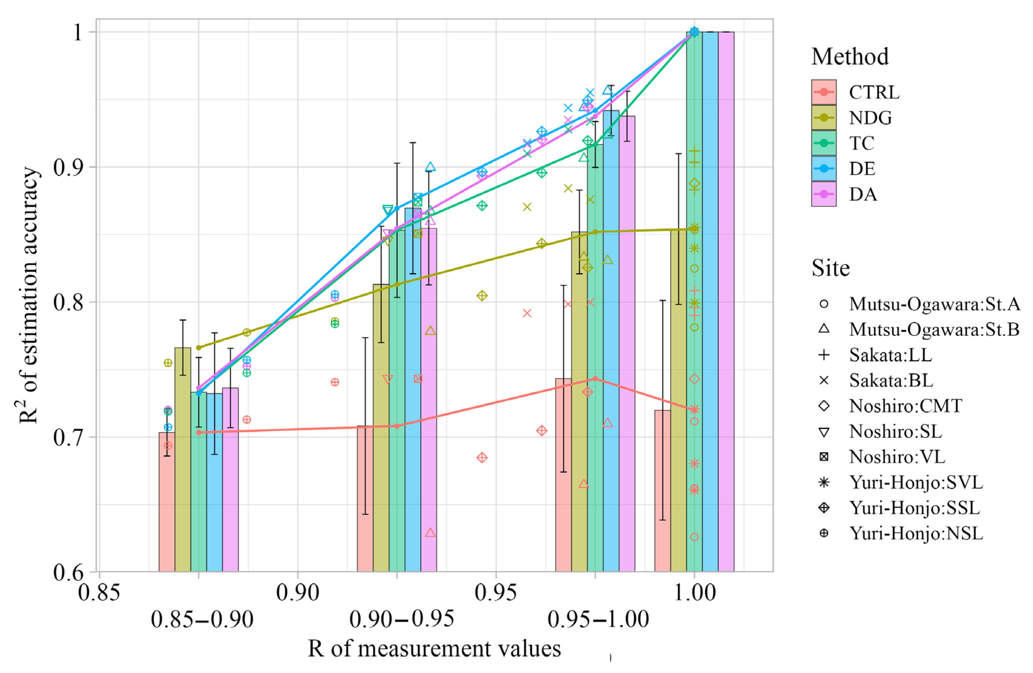
| Bin of R | 0.85–0.90 | 0.90–0.95 | ||||||||
|---|---|---|---|---|---|---|---|---|---|---|
| # of Cases | 2 | 5 | ||||||||
| Method | CTRL | NDG | TC | DE | DA | CTRL | NDG | TC | DE | DA |
| Mean [%] | 0.70 | 0.77 | 0.73 | 0.73 | 0.74 | 0.71 | 0.81 | 0.85 | 0.87 | 0.85 |
| Std.Dev. [%] | 0.01 | 0.02 | 0.02 | 0.04 | 0.02 | 0.05 | 0.03 | 0.04 | 0.04 | 0.03 |
| Bin of R | 0.95–1.00 | 1.00 (Only reference points) | ||||||||
| # of cases | 7 | 10 | ||||||||
| Method | CTRL | NDG | TC | DE | DA | CTRL | NDG | TC | DE | DA |
| Mean [%] | 0.74 | 0.85 | 0.92 | 0.94 | 0.94 | 0.72 | 0.85 | 1.00 | 1.00 | 1.00 |
| Std.Dev. [%] | 0.05 | 0.02 | 0.01 | 0.01 | 0.01 | 0.06 | 0.04 | 0.00 | 0.00 | 0.00 |
Disclaimer/Publisher’s Note: The statements, opinions and data contained in all publications are solely those of the individual author(s) and contributor(s) and not of MDPI and/or the editor(s). MDPI and/or the editor(s) disclaim responsibility for any injury to people or property resulting from any ideas, methods, instructions or products referred to in the content. |
© 2025 by the authors. Licensee MDPI, Basel, Switzerland. This article is an open access article distributed under the terms and conditions of the Creative Commons Attribution (CC BY) license (https://creativecommons.org/licenses/by/4.0/).
Share and Cite
Maruo, T.; Ohsawa, T. Wind Estimation Methods for Nearshore Wind Resource Assessment Using High-Resolution WRF and Coastal Onshore Measurements. Wind 2025, 5, 17. https://doi.org/10.3390/wind5030017
Maruo T, Ohsawa T. Wind Estimation Methods for Nearshore Wind Resource Assessment Using High-Resolution WRF and Coastal Onshore Measurements. Wind. 2025; 5(3):17. https://doi.org/10.3390/wind5030017
Chicago/Turabian StyleMaruo, Taro, and Teruo Ohsawa. 2025. "Wind Estimation Methods for Nearshore Wind Resource Assessment Using High-Resolution WRF and Coastal Onshore Measurements" Wind 5, no. 3: 17. https://doi.org/10.3390/wind5030017
APA StyleMaruo, T., & Ohsawa, T. (2025). Wind Estimation Methods for Nearshore Wind Resource Assessment Using High-Resolution WRF and Coastal Onshore Measurements. Wind, 5(3), 17. https://doi.org/10.3390/wind5030017