Reflection of Wind Turbine Noise from Rough Ground Using 3D Multiple Scattering Theory

Abstract

Ground roughness is investigated for its influence on the propagation of wind turbine noise by using a proposed multiple scattering theory to predict the reflection of sound waves from a deterministic distribution of hemispheres. By using a distribution of hemispheres as an approximation for a realistic rough ground, a semi-analytical formulation for the reflected sound pressure is possible. Experiments are conducted within the University of Hull’s anechoic chamber and the results are compared against predictions from the proposed theory. Good agreement between the results is shown. The proposed multiple scattering theory also gives results consistent with a three-dimensional boundary element method, while having significantly shorter computation times and smaller memory requirements. Furthermore, results remain accurate up to the point where the radii of the hemispheres are comparable to the wavelengths of interest, which means that the scattering effect can be investigated more completely. When the proposed theory was applied to the unique source–receiver geometry of a wind turbine and a human height receiver, the excess attenuation calculated over an array of receivers showed significant fluctuations in sound pressure which were attributed to the ground roughness. Further works aim to incorporate weak refraction effects and ground absorption to analyze the relative influence of different parameters.

1. Introduction

The noise generated by wind turbines can be a major hinderance to the public acceptance of the technology [1]. Aspects of the current framework in the UK for controlling wind turbine-generated noise [2] have been described as outdated in light of developments in the literature and technology [3]. The noise that is generated by wind turbines is, at a minimum, cause for annoyance, despite the levels being modest compared to other sources like traffic noise [4]. Therefore, there may be some public benefit in being able to accurately predict and report sound levels around a wind turbine or wind farm. Furthermore, wind turbine sound propagation models are beneficial because they could be used practically during the micro-siting process.

Understanding how sound reflects from the ground is an important aspect of predicting sound levels outdoors, especially when the ground is uneven as this can result in a scattering effect. In the context of outdoor sound propagation, scattering may be described as the diffraction of sound at a rough surface, where the magnitude of the scattering effect is dependent on variables such as the frequency, the profile of the rough surface, and the source–receiver geometry.

There are different methods for incorporating the ground roughness, and its scattering effect, when predicting outdoor sound levels. A popular option is to use an effective impedance model in the ground boundary conditions of some Parabolic Equation (PE) method, say the Crank–Nicholson Parabolic Equation (CNPE) method [5]. These methods have been used to highlight that the scattering from a rough ground surface can significantly affect the propagation of sound from wind turbines [6,7]. An effective impedance models the scattering effect as an intrinsic property of the ground surface, in the sense that a rough ground may be treated as a flat one of modified impedance. However, effective impedances are often only valid when the wavelength is large comparative to the dimensions of the rough surface (or vice versa). Using an effective impedance outside this condition can lead to prediction errors [8]. Under such cases, scattering is mainly in the forward specular direction [9,10]. As the wavelength becomes comparative to the dimensions of a rough surface, scattering in non-specular directions dominates [11], and most effective impedance models are not applicable. Alternative methods include PE methods that directly incorporate surface roughness. For example, the generalized terrain parabolic equation (GTPE) method [12,13]. The GTPE method, as outlined by Sack and West [14], uses a terrain following coordinate transformation to account for a surface roughness. However, there are strict limits on the roughness slope. For the GTPE, the limit is a local slope of up to 30° [15].

A less common method, in the context of wind turbine noise prediction, is developing a multiple scattering theory (MST). MSTs are analytical or semi-analytical methods for predicting the scattered sound pressure from a deterministic rough surface and are generally more efficient than numerical methods like boundary element methods (BEMs). Linton and Martin [16,17] and Linton and Evans [18] have worked extensively on MSTs for both cylinders and spheres which are deterministically placed in a medium where some sound wave is propagating. Shin [19] developed an MST for spheres in the presence of reflecting surfaces and corners. This was achieved by solving for the unknown coefficients of outgoing waves from image objects which were related to the real counterpart using image conditions. Spherical and planar incidence were both accounted for, and the reflecting planes were treated either as sound hard or sound soft.

MSTs for spheres in the presence of an impedance ground surface (or outdoor ground surface) was studied by Li, Lui, and Frommer [20]. They focused on the case of a single sphere suspended close to a ground surface, wherein the scattering is between the sphere and the ground surface. They accounted for the acoustical properties of the ground by incorporating the Weyl–van der Pol formula and the spherical wave reflection coefficient in their formulation. Other works have developed and used MSTs to investigate the multiple scattering from rigid cylinders in the presence of a ground plane [21,22]. Boulanger, Attenborough, Qin, and Linton [23] developed formulations for the scattering of sound pressure from distributions of semi-cylinders on flat, hard planes. This particular two-dimensional MST has been used to investigate noise reduction with interesting results, showing that there is promising applicability for noise reduction if the receiver is low [24]. In fact, it is understood that a rough ground surface (both random and periodic) can be used positively for noise reduction [25,26].

Distributions of hemispheres on a flat plane can be a reasonable approximation for a realistic rough ground surface and may be used to investigate the reflection of wind turbine noise. To the best of the authors’ knowledge, there has not been an MST which accounts for multiple hemispheres placed onto a flat reflecting plane. Therefore, it is the purpose of this paper to propose such a theory, validate it, and then apply the theory to the prediction of wind turbine noise propagation over a rough ground.

Section 2 describes the theoretical formulations of the proposed MST. Section 3 outlines the experimental methods used to gather data for the purpose of validating the proposed MST. Furthermore, Section 4 outlines the key aspects of a three-dimensional boundary element method. Section 5 provides comparisons between the results from the experiments, BEMs, and the proposed MST. The validity of the MST is then discussed. Section 6 describes how MSTs can be used in the context of wind turbine noise propagation, wherein the parameters of some case studies are described, and the results are shown. Finally, in Section 7, the results are discussed and conclusions drawn. Also, some further work is proposed.

2. Multiple Scattering Theory

Consider $N$ hemispheres $H_j$ with radii $a_j$ and complex admittance (inverse of impedance) ${\beta }_j$ that are all located on a flat reflecting plane. The sound pressure $p$ exterior to the hemispheres and the flat surface satisfies the three-dimensional Helmholtz equation

$${\nabla }^{2}p+k^{2}p=0.$$

(1)

${\nabla }^2$ is the Laplacian operator in spherical polar coordinates and $k$ is the wavenumber. A point source is positioned at ${\mathit{x}}_o$ and a receiver is positioned at ${\mathit{x}}_r$. Therefore, the vector from source directly to the receiver is ${\mathit{r}}_{or}=\left(r_{or},{\theta }_{or},{\varphi }_{or}\right)$.

An expression for an incident wave is needed. An outgoing spherical wave in free space may be given as

$$p_{inc}=h_0^{\left(1\right)}\left(k{r}_{or}\right),$$

(2)

where $h_0^{\left(1\right)}$ is a spherical Hankel function of first kind and zeroth order [27], and is the linear combination of the solutions to the Helmholtz equation when separated into radial variables [28]. This gives an outgoing wave in the $r_{or}$ direction. Using an addition theorem for spherical Hankel functions [29] (p. 89), the incident wave as a function of $r_{or}$ can be given in terms of the position of one of the hemispheres, say hemisphere $H_j$. We establish a spherical polar coordinate system with origins $O_j$ at the centre of each hemisphere, such that the vector between a hemisphere center and the receiver is ${\mathit{r}}_{jr}=\left(r_{jr},{\theta }_{jr},{\varphi }_{jr}\right)$. Furthermore, with ${\mathit{r}}_{oj}=\left(r_{oj},{\theta }_{oj},{\varphi }_{oj}\right)$ being the vector between the source and hemisphere $H_j$, we write ${\mathit{r}}_{or}={\mathit{r}}_{oj}+{\mathit{r}}_{jr}$ and the incident wave can be given by

$$p_{inc}={\displaystyle \sum }_{n=0}^{\infty }{\displaystyle \sum }_{m=-n}^{n}4\pi {\left(-1\right)}^n{h}_n^{\left(1\right)}\left(k{r}_{oj}\right)\overline{Y_n^m\left({\theta }_{oj},{\varphi }_{oj}\right)}{j}_n\left(k{r}_{jr}\right)Y_n^m\left({\theta }_{jr},{\varphi }_{jr}\right),$$

(3)

subject to the condition $r_{jr}<r_{oj}$. $j_n$ is the spherical Bessel function [30], and $Y_n^m$ is the normalized spherical harmonic [31]. The overbar indicates the complex conjugate.

Assuming the reflecting plane is sound hard, an expression for the reflected wave can be given using the following method of images. The reflected wave is taken as a spherical wave originating from the image source, ${\mathit{x}}_i$. The image source is the mirror of the point source in the $xy$ plane such that, in Cartesian coordinates, ${\mathit{x}}_o=\left(x_o,y_o,z_o\right)$ and ${\mathit{x}}_i=\left(x_0,y_o,-z_o\right)$. This reflected wave is given by

$$p_{ref}=h_0^{\left(1\right)}\left(k{r}_{ir}\right),$$

(4)

where ${\mathit{r}}_{ir}=\left(r_{ir},{\theta }_{ir},{\varphi }_{ir}\right)$ is the vector from the image source to the receiver. With ${\mathit{r}}_{ij}=\left(r_{ij},{\theta }_{ij},{\varphi }_{ij}\right)$ being the vector between the image source and hemisphere $H_j$,

$$p_{ref}={\displaystyle \sum }_{n=0}^{\infty }{\displaystyle \sum }_{m=-n}^{n}4\pi {\left(-1\right)}^n{h}_n^{\left(1\right)}\left(k{r}_{ij}\right)\overline{Y_n^m\left({\theta }_{ij},{\varphi }_{ij}\right)}{j}_n\left(k{r}_{jr}\right)Y_n^m\left({\theta }_{jr},{\varphi }_{jr}\right).$$

(5)

It is supposed that the scattered sound pressure is the sum of contributions from each hemisphere. From each hemisphere, the scattered waves can be expressed as the linear combination of product solutions for the separated equations of the Helmholtz equation in the spherical polar coordinates. Furthermore, unknown coefficients, ${𝒸}_{jn}^m$, are attached to the solution, which it is the objective to solve for.

$$p_{sca}={\displaystyle \sum }_{j=1}^N{\displaystyle \sum }_{n=0}^{\infty }{\displaystyle \sum }_{m=-n}^n{𝒸}_{jn}^m{h}_n^{\left(1\right)}\left(k{r}_{jr}\right)Y_n^m\left({\theta }_{jr},{\varphi }_{jr}\right).$$

(6)

Considering each hemisphere, $H_j$, and some other hemisphere, say $H_s,$ the vectors between them may be given as ${\mathit{h}}_{js}=\left(h_{js},{\theta }_{js},{\varphi }_{js}\right)$. Another addition theorem, for spherical wavefunctions [29] (p. 90), is then used to express the scattered component at each jth hemisphere, in terms of the sth hemisphere.

$$p_{sca}={\displaystyle \sum }_{n=0}^{\infty }{\displaystyle \sum }_{m=-n}^n\left\{{𝒸}_{sn}^m{h}_n^{\left(1\right)}\left(k{r}_{sr}\right)Y_n^m\left({\theta }_{sr},{\varphi }_{sr}\right)+{\displaystyle \sum }_{\begin{array}{c}j=1\\ j\ne s\end{array}}^N{𝒸}_{jn}^m{\displaystyle \sum }_{\nu =0}^{\infty }{\displaystyle \sum }_{\mu =-\nu }^{\nu }{𝒮}_{n\nu }^{m\mu }\left({\mathit{h}}_{js}\right)j_{\nu }\left(k{r}_{sr}\right)Y_{\nu }^{\mu }\left({\theta }_{sr},{\varphi }_{sr}\right)\right\}$$

(7)

subject to ${\mathit{r}}_{jr}={\mathit{h}}_{js}+{\mathit{r}}_{sr}$ and $r_{sr}<h_{js}$. ${𝒮}_{n\nu }^{m\mu }\left({\mathit{h}}_{js}\right)$ is a complicated function associated with the addition theorem. Only the necessary details are outlined here,

$$S_{n\nu }^{m\mu }\left({\mathit{h}}_{js}\right)=4\pi i^{\nu -n}{\displaystyle \sum }_{q=\left|n-\nu \right|}^{\left(n+\nu \right)}{i}^q{\left(-1\right)}^m{h}_q\left(k{h}_{js}\right)\overline{Y_q^{\mu -m}\left({\theta }_{js},{\varphi }_{js}\right)}𝒢\left(n,m;\nu ,-\mu ;q\right).$$

(8)

The sum in $q$ must be taken in steps of 2 and $𝒢\left(n,m;\nu ,-\mu ;q\right)$ is a gaunt coefficient [29,32]. Also, note that ${\theta }_{js}\equiv pi/2$. The unknown coefficients in $c_{jn}^m$ may be moved inside the sums in $\nu$ and $\mu$ for ${𝒸}_{j\nu }^{\mu }$.

$$p_{sca}={\displaystyle \sum }_{n=0}^{\infty }{\displaystyle \sum }_{m=-n}^n\left\{{𝒸}_{sn}^m{h}_n^{\left(1\right)}\left(k{r}_{sr}\right)Y_n^m\left({\theta }_{sr},{\varphi }_{sr}\right)+{\displaystyle \sum }_{\begin{array}{c}j=1\\ j\ne s\end{array}}^N{j}_n\left(k{r}_{sr}\right)Y_n^m\left({\theta }_{sr},{\varphi }_{sr}\right){\displaystyle \sum }_{\nu =0}^{\infty }{\displaystyle \sum }_{\mu =-\nu }^{\nu }{𝒮}_{\nu n}^{\mu m}\left({\mathit{h}}_{js}\right){𝒸}_{j\nu }^{\mu }\right\}$$

(9)

Therefore, the total sound pressure is the sum of the incident, reflected and scattered components, $p=p_{inc}+p_{ref}+p_{sca}$. Expressing each component in terms of hemisphere $H_s$ gives

$$\begin{gathered} p_{inc}+p_{ref}+p_{sca}= \\ {\displaystyle \sum }_{n=0}^{\infty }{\displaystyle \sum }_{m=-n}^n\left\{4\pi {\left(-1\right)}^n{j}_n\left(k{r}_{sr}\right)Y_n^m\left({\theta }_{sr},{\varphi }_{sr}\right)\left[h_n^{\left(1\right)}\left(k{r}_{os}\right)\overline{Y_n^m\left({\theta }_{os},{\varphi }_{os}\right)}+h_n^{\left(1\right)}\left(k{r}_{is}\right)\overline{Y_n^m\left({\theta }_{is},{\varphi }_{is}\right)}\right] \\ +{𝒸}_{sn}^m{h}_n^{\left(1\right)}\left(k{r}_{sr}\right)Y_n^m\left({\theta }_{sr},{\varphi }_{sr}\right)+{\displaystyle \sum }_{\begin{array}{c}j=1\\ j\ne s\end{array}}^N{j}_n\left(k{r}_{sr}\right)Y_n^m\left({\theta }_{sr},{\varphi }_{sr}\right){\displaystyle \sum }_{\nu =0}^{\infty }{\displaystyle \sum }_{\mu =-\nu }^{\nu }{𝒮}_{\nu n}^{\mu m}\left({\mathit{h}}_{js}\right){𝒸}_{j\nu }^{\mu }\right\} \end{gathered}$$

(10)

Furthermore, applying an impedance boundary condition,

$${\displaystyle \frac{𝜕p}{𝜕n}}-ik{\beta }_{s}p=0,$$

(11)

on the surface of the sth hemisphere, at ${\mathrm{r}}_{\mathrm{sr}}=a_s$, gives an infinite set of equations. $n$ is the normal to the hemisphere surface. The infinite sums are truncated at some value $M$, so that the set of equations may be solved numerically. The truncated set of equations is given by

$$\begin{gathered} {𝒸}_{sn}^m+{\displaystyle \sum }_{\begin{array}{c}j=1\\ j\ne s\end{array}}^N{ℬ}_{sn}{\displaystyle \sum }_{\nu =0}^{\mathrm{M}}{\displaystyle \sum }_{\mu =-\nu }^{\nu }{𝒮}_{\nu n}^{\mu m}\left({\mathit{h}}_{js}\right){𝒸}_{j\nu }^{\mu }= \\ -{ℬ}_{sn}4\pi {\left(-1\right)}^n\left[h_n^{\left(1\right)}\left(k{r}_{os}\right)\overline{Y_n^m\left({\theta }_{os},{\varphi }_{os}\right)}+h_n^{\left(1\right)}\left(k{r}_{is}\right)\overline{Y_n^m\left({\theta }_{is},{\varphi }_{is}\right)}\right], \\ \begin{array}{c}for s=1,2,\dots ,N, n=0,1,\dots ,M, m=-n,\dots ,+n,\end{array} \end{gathered}$$

(12)

where

$${ℬ}_{sn}={\displaystyle \frac{j_n^{\prime }\left(k{a}_s\right)+ik{\beta }_s{j}_n\left(k{a}_s\right)}{h_n^{{\left(1\right)}^{\prime }}\left(k{a}_s\right)+ik{\beta }_s{h}_n\left(k{a}_s\right)}}.$$

(13)

Once the unknown coefficients are determined, using Equations (2), (4), and (6), the total pressure at the receiver position can be calculated. For sound hard hemispheres, the limit can be taken as ${\beta }_s\to 0$. The excess attenuation can then be calculated using the following formula:

$$EA \left(dB\right)=20{\log }_{10}\left({\displaystyle \frac{\left|p_{inc}+p_{ref}+p_{sca}\right|}{\left|p_{inc}\right|}}\right).$$

(14)

Excess attenuation is used because it highlights the ground effect.

3. Experiment Methods

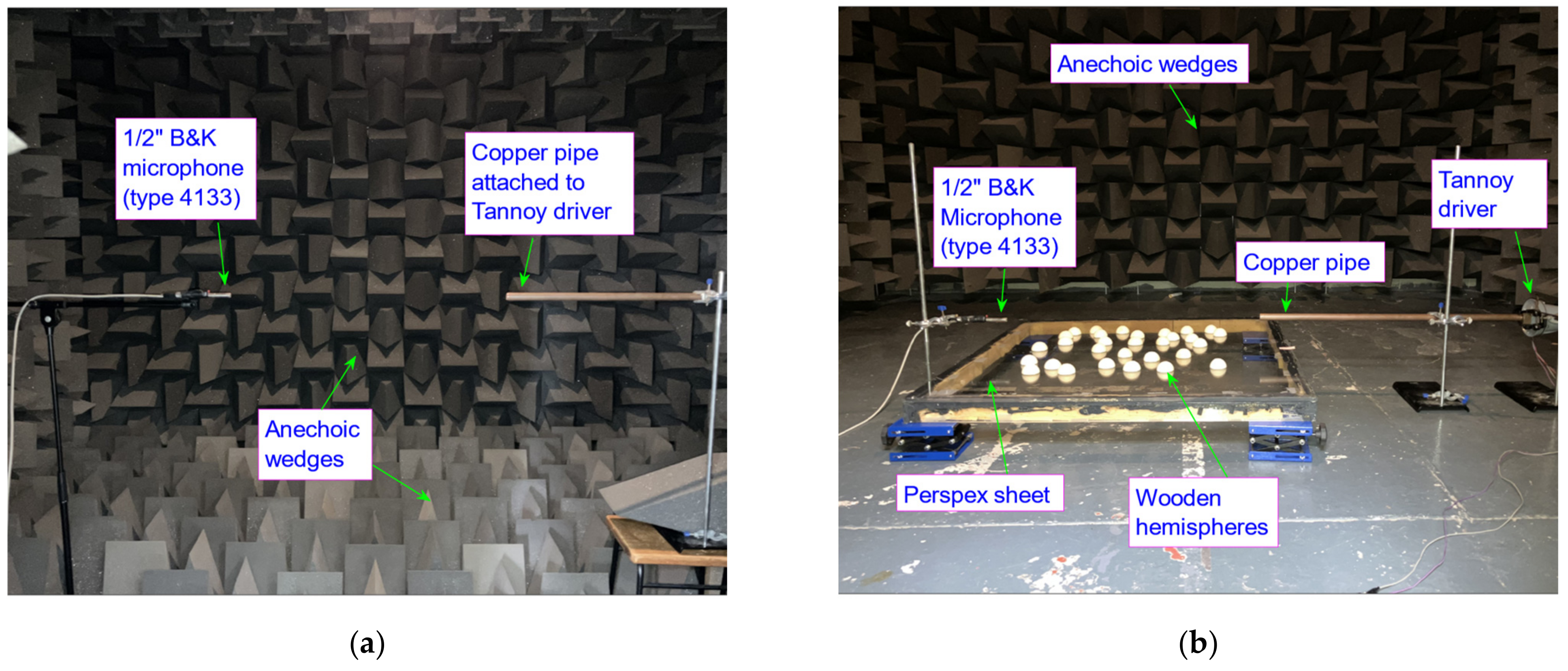
To validate the theory, measurements of the reflection of sound from distributions of hemispheres were taken within the University of Hull’s anechoic chamber.

A 1 ${\mathrm{m}}^2$ Perspex sheet was placed in the center of the anechoic chamber balanced on its corners by 4 jacks which kept the sheet level. A half inch B&K (type 4133) condenser microphone was used for the receiver. With the center of the Perspex sheet being the origin of a Cartesian coordinate space, the center of the microphone was positioned at $\left(-0.4, 0, 0.1\right)$ m. Similarly, a Tannoy driver, fitted with a 1 m copper tube (0.02 m diameter), was used to represent a point source. The center of the end of the copper tube was positioned at $\left(0.4, 0, 0.1\right)$ m. The source–receiver geometry was chosen specifically because the first ground interference dip was prominent in the excess attenuation spectra. Various distributions of 30 hemispheres, all 0.025 m radius, were generated using pseudorandom number generators in MATLAB (version R2024b) for the x and y coordinates on the reflecting plane. The pseudorandom number generator is not truly random but succeeds in creating distributions of hemispheres which appear random. The coordinates were limited to a 0.6 m² area, with the center of the Perspex sheet being the origin of the coordinate space for reference to the hemisphere positions.

Then, one of the distributions of hemispheres was chosen and carefully placed on the Perspex sheet. The hemispheres used were solid wooden hemispheres, all 0.025 m in radius. Also, to calculate the excess attenuation, free field measurements were necessary. For these measurements, a free field was created in the anechoic chamber by filling the floor with anechoic wedges and suspending the source and receivers above the wedges at a sufficient height. The distance between the source and receiver was kept at 0.8 m. The experiments for the free field and for one of the roughness distributions are shown in Figure 1.

Once the apparatus was set up, maximum length sequence (MLS) signals were used for gaining the impulse response of the system. This is a method developed by Schroeder [33]. MLS signals are pseudo-random sequences of +1 and −1. MLS signals are advantageous because they have a flat frequency spectrum from the DC term (near 0 Hz) to the Nyquist frequency. Furthermore, by using MLS signals, we were able to achieve a better signal-to-noise ratio (SNR) than if acoustic pulses were used. An MLS signal, 65,535 points in length, was generated on a PC with a 40 kHz clock rate. This allows for analysis of frequencies up to 20 kHz. The MLS signal was amplified by a Sony stereo amplifier (model TA-FE33OR) and emitted by the Tannoy driver. Following methods described by Walker [34], the MLS signal was repeated twice, and the second period of the signal was recorded and processed. Signals were received by a half inch B&K (model 4133) condenser microphone, amplified by a B&K amplifier (model 2609), and the data acquired by a National Instruments 5911 Series Data Acquisition Card (DAQ). The received signal was sampled at 40 kHz (same at the MLS clock frequency). Then, using the National Instruments LABVIEW virtual oscilloscope software (version 2.1), the digital signals were saved where postprocessing (calculating the impulse responses) could be conducted externally. Then, as detailed by Chu [35], the impulse responses were calculated through cross-correlation of the input MLS signal and the received system response. For each distribution of hemispheres that was chosen, 15 impulse responses were averaged to improve the signal-to-noise ratio. The frequency transform was then calculated using discrete Fourier transforms [36].

4. Boundary Element Method

A boundary element method code was written in MATLAB for simulating the scattering of sound waves from a three-dimensional roughness. We followed the methods from Chandler-Wilde [37] to derive the boundary integral equation; however, the method was applied to the three-dimensional problem rather than the two-dimensional. Also, a sound hard (Neumann) boundary condition was used for simplicity. For a point source at ${\mathit{x}}_o$, a receiver at ${\mathit{x}}_r$ and points on the sound hard hemisphere boundary, $S$, at ${\mathit{x}}_s$, the acoustic pressure, $p$, can be given by

$$ϵ\left({\mathit{x}}_r\right)p\left({\mathit{x}}_r\right)=G\left({\mathit{x}}_r,{\mathit{x}}_o\right)+\underset{S}{{\displaystyle \int }}{\displaystyle \frac{G\left({\mathit{x}}_s,{\mathit{x}}_r\right)}{\partial n\left({\mathit{x}}_s\right)}}p\left({\mathit{x}}_s\right)dS\left({\mathit{x}}_s\right), for {\mathit{x}}_s on S,$$

(15)

where $n$ is the normal direction outwards from the boundary $S$ and $ϵ\left({\mathit{x}}_r\right)$ is a factor dependent on receiver position. $G\left({\mathit{x}}_r,{\mathit{x}}_o\right)$ is the Green’s function for the sound field above an acoustically hard plane in three-dimensions. Following methods in Wright [38],

$$G\left({\mathit{x}}_r,{\mathit{x}}_o\right)=-{\displaystyle \frac{\mathit{exp}\left(ik\left|{\mathit{x}}_r-{\mathit{x}}_o\right|\right)}{4\pi \left|{\mathit{x}}_r-{\mathit{x}}_o\right|}}-{\displaystyle \frac{\mathit{exp}\left(ik\left|{\mathit{x}}_r-{\mathit{x}}_i\right|\right)}{4\pi \left|{\mathit{x}}_r-{\mathit{x}}_i\right|}}.$$

(16)

By using this method, there is no need to discretize the flat ground surrounding the roughness which saves computation time significantly.

For the boundary element method, the boundary was discretized into a set of boundary elements and the corresponding discretized boundary integral equation was solved approximately by assuming the solution to be a polynomial of zeroth order on the surface of each boundary element. A point collocation method was used to determine the pressure at the centroids of the boundary elements as a solution to a set of linear equations. The collocation method creates singularities in the Green’s function at a series of points, ${\mathit{x}}_r={\mathit{x}}_o$ and ${\mathit{x}}_r={\mathit{x}}_i$, which can be avoided by setting the boundary integral at that point to zero, as detailed by Chandler-Wilde and Langdon [39]. Furthermore, integrals on the surface of each boundary element were approximated using the midpoint rule. Using this scheme, it was possible to approximate the scattered acoustic pressure from a rough surface, where the accuracy increases with refinement of the boundary element sizes. A convergence test was conducted for a distribution of 30 hemispheres of 0.025 m radius over one-third octave band frequencies from 500 Hz to 16 kHz. The results show the boundary element areas must be at least one-fifth the wavelength squared for consistent results.

5. Validation

5.1. Comparison to Measurements

Figure 2 shows comparisons between the excess attenuation from the proposed multiple scattering theory and from the experiments detailed in Section 3. In order to compare measurements to the proposed theory, a truncation parameter was required. From a convergence test on one of the distributions of hemispheres, the truncation parameter of $M=7$ was sufficient for consistent results up to 16 kHz. Since the temperature in the lab was $~11°$, the sound speed used in the multiple scattering theory, and the boundary element method, was 337.8338 m/s. Out of the 30 distributions of hemispheres, distributions 2 and 3 were chosen. The agreement is as the theory manages to capture the ground interference dips at the correct frequency. Also, the fluctuations in the excess attenuation across the frequency spectrum seem to be consistent with the measured data. However, in Figure 2b it is clear that the magnitude of the ground interference dip is overpredicted by the multiple scattering theory. The theory appears to remain consistent beyond the point at which the wavelength is equal to the hemisphere radius, which is about 13,513 Hz in this case. Overall, in comparison to the measured data, the proposed MST gives consistent results.

5.2. Comparison to BEM

Figure 3 shows comparisons between the proposed multiple scattering theory and the boundary element method. The boundary element method code on MATLAB was run on the University of Hull’s high-performance computer, where the excess attenuation is calculated over 100 logarithmically spaced frequency points between 500 Hz and 16 kHz. While results for all the distributions are available, a select few are shown here. The discrepancies between the boundary element method and the new multiple scattering theory are very small. There are some more obvious discrepancies in the boundary element method; however, this can be expected due to the approximations which were made. Furthermore, on the high-performance computer, the time taken for the boundary element method to calculate the excess attenuation was roughly 6 min and 30 s per frequency interval. The multiple scattering theory took just under 2 s per frequency interval on a personal laptop, making it around 200 times quicker. Furthermore, in terms of memory, the multiple scattering theory requires very little memory compared to the boundary element method. For both the boundary element method and the multiple scattering theory, most of the memory is in the square matrix of coefficients resulting from the sets of equations in Equation (12) and from the collocation method. For the multiple scattering theory, the size of the matrix is given by $N^2\ast {\left(M+1\right)}^4$, which corresponds to roughly 29.5 MB for 30 hemispheres, a truncation parameter of 7 using double precision values. This is much smaller when compared to the boundary element method which requires roughly 8 GB. Overall, the proposed MST gives consistent results to the BEM at much faster speed.

6. Application Toward Wind Turbine Noise Prediction

6.1. Parameters of Wind Turbine Noise Case Study

With the proposed MST validated by comparison to measurements and numerical simulations (BEM), the next step is to apply the MST practically towards investigating the reflection of wind turbine noise from a rough ground. Therefore, this section is dedicated to investigating the propagation of wind turbine noise over a rough, or hilly, ground approximated by a distribution of hemispheres. Furthermore, since the aim is to investigate the scattering effect of the rough surface, the hemispheres and reflecting plane are taken as sound hard. This ensures that any significant results can be attributed to the scattering effect alone.

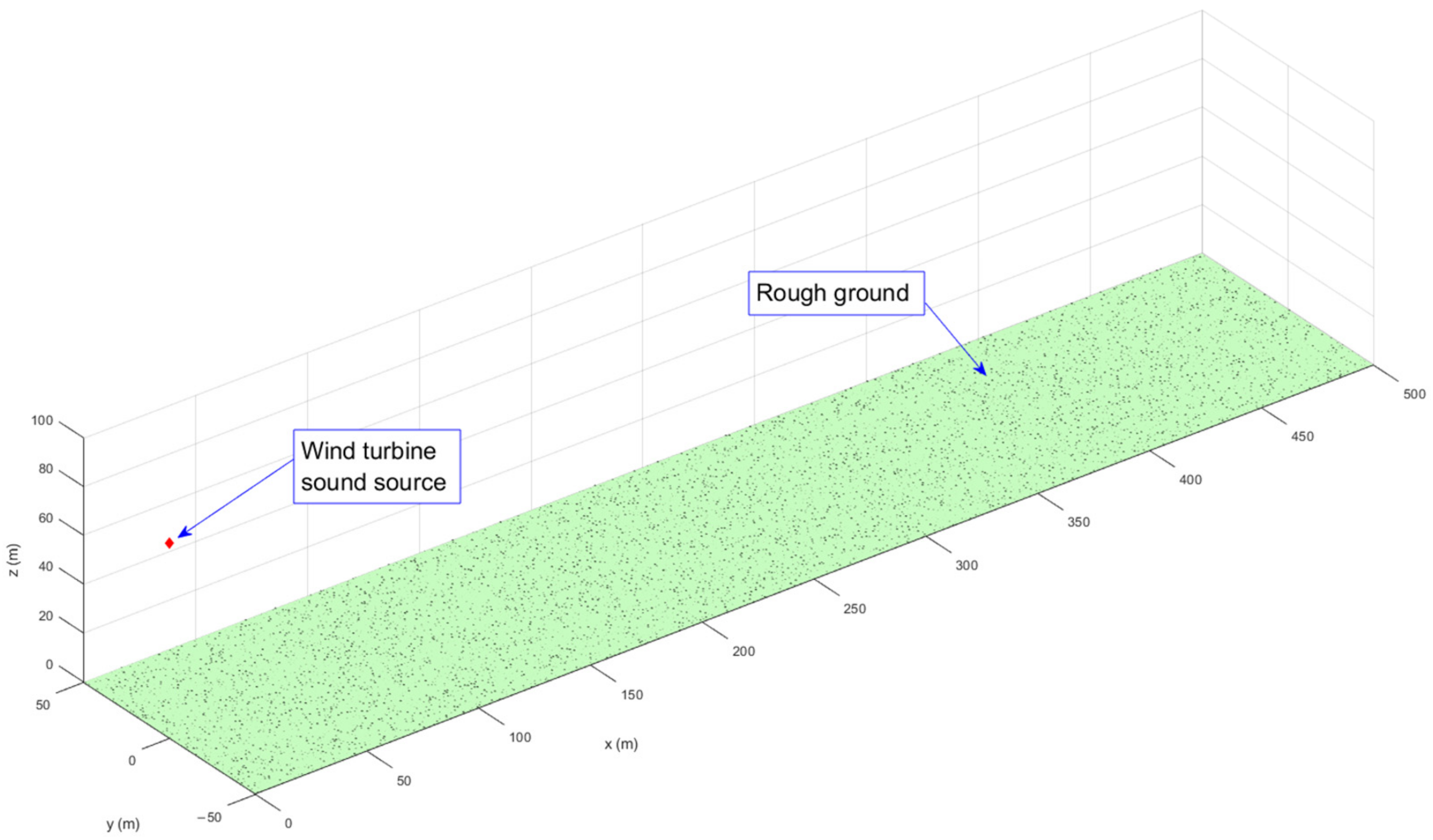
The coordinates of 10,000 hemispheres are generated by a pseudorandom number generator in MATLAB. The pseudorandom number generator is not truly random but succeeds in creating distributions of hemispheres which appear random. The hemisphere radii are generated using the same pseudorandom number generator. The x and y coordinates of the hemisphere centers are generated between specified intervals on the x and y axis, those being from 0 m to 500 m in the x direction and −50 m to 50 m in the y direction. Outside the area described, the ground is assumed flat. Furthermore, the hemisphere radii are generated between specified intervals from 0.1 m to 0.5 m. This creates a rough ground that has a varying bumpiness. A maximum radius is given to not limit the frequencies that can be investigated. After all, the scattering theory has not been validated for hemisphere radii which are much larger than the wavelengths of interest. Therefore, a maximum radius of 0.5 m limits the frequencies to roughly under 680 Hz. A minimum radius is given because a very small roughness at the described frequencies is expected to have only a small scattering effect. The hemisphere radii are generated first; then, a hemisphere coordinate is generated where it is checked as to whether the hemisphere overlaps with another. If it does, a new coordinate is generated.

In the domain created where some distribution of hemispheres lies, a point source is suspended at position $\left(0, 0, 80\right)$ m, as 80 m is a sensible height for an onshore wind turbine. Furthermore, as a receiver is positioned further into the far field, $kr\gg 1$, a point source becomes a more appropriate approximation of a wind turbine sound source [40]. Closer to the sound source, a point source approximation instead of an extended source model can lead to some discrepancies in interference dips [41,42]. However, for engineering applications, the point source approximation seems a reasonable approach and has been recommended for wind turbine noise prediction schemes [43].

Receiver points are positioned in 1 m intervals over the entire 500 m by 100 m area at a height of 1.7 m. The height is chosen to represent a person’s perception of the sound generated by the wind turbine. Finally, the frequencies investigated are octave band frequencies 63 Hz, 125 Hz, 250 Hz, and 500 Hz. While these may not be the dominant frequencies emitted from wind turbines [44], lower frequency noise propagates much further in the atmosphere than higher frequencies. Figure 4 shows a distribution of hemispheres generated using the methods described. Also, the location of the point source is outlined.

To use the multiple scattering theory, a truncation parameter needs to be chosen. A convergence test is conducted for a distribution of hemispheres ranging from 0.1 m to 0.5 m in radius. It was found that for the octave band frequencies, 65 Hz, 125 Hz, 250 Hz, and 500 Hz, truncation parameters of 1, 1, 2, 2, respectively, were sufficient. When all the parameters were set, the simulations were run on the University of Hull’s High-Performance Computer. The excess attenuation is calculated again using Equation (14).

6.2. Results from Wind Turbine Noise Case Study

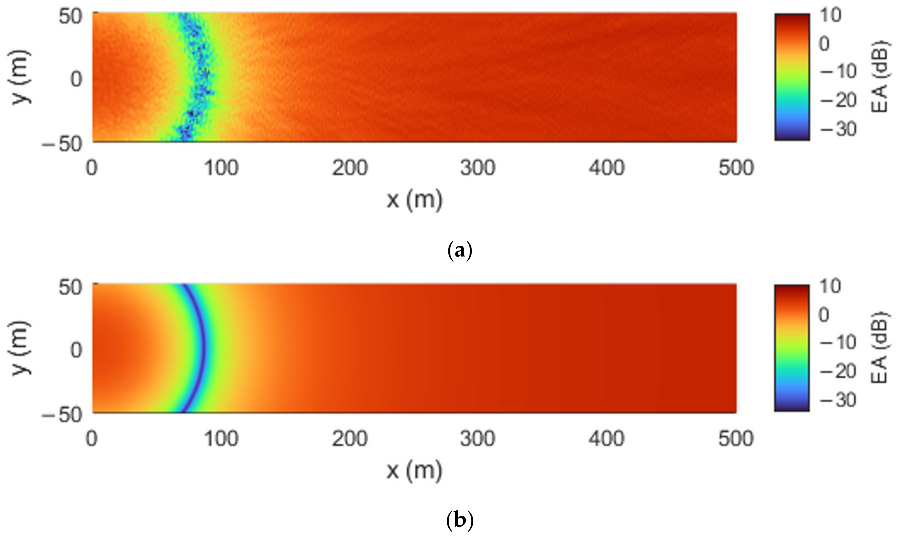
Figure 5, Figure 6, Figure 7 and Figure 8 show the excess attenuation at frequencies of 63 Hz, 125 Hz, and 500 Hz, respectively. The excess attenuation calculated for the equivalent case, however with a perfectly reflecting flat ground surface, are shown also for comparison between the results and to highlight the significance of the scattering effect.

In Figure 5a, there is not a large difference between the results shown in Figure 5b. However, the small, seemingly random patterns in the excess attenuation do indicate that some interference caused by scattered sound waves. We note that, at the frequency of 63 Hz, the wavelength is over ten times larger than the largest hemisphere radius (0.5 m). Therefore, the indication that the scattering mainly is in the forward specular direction is not necessarily surprising.

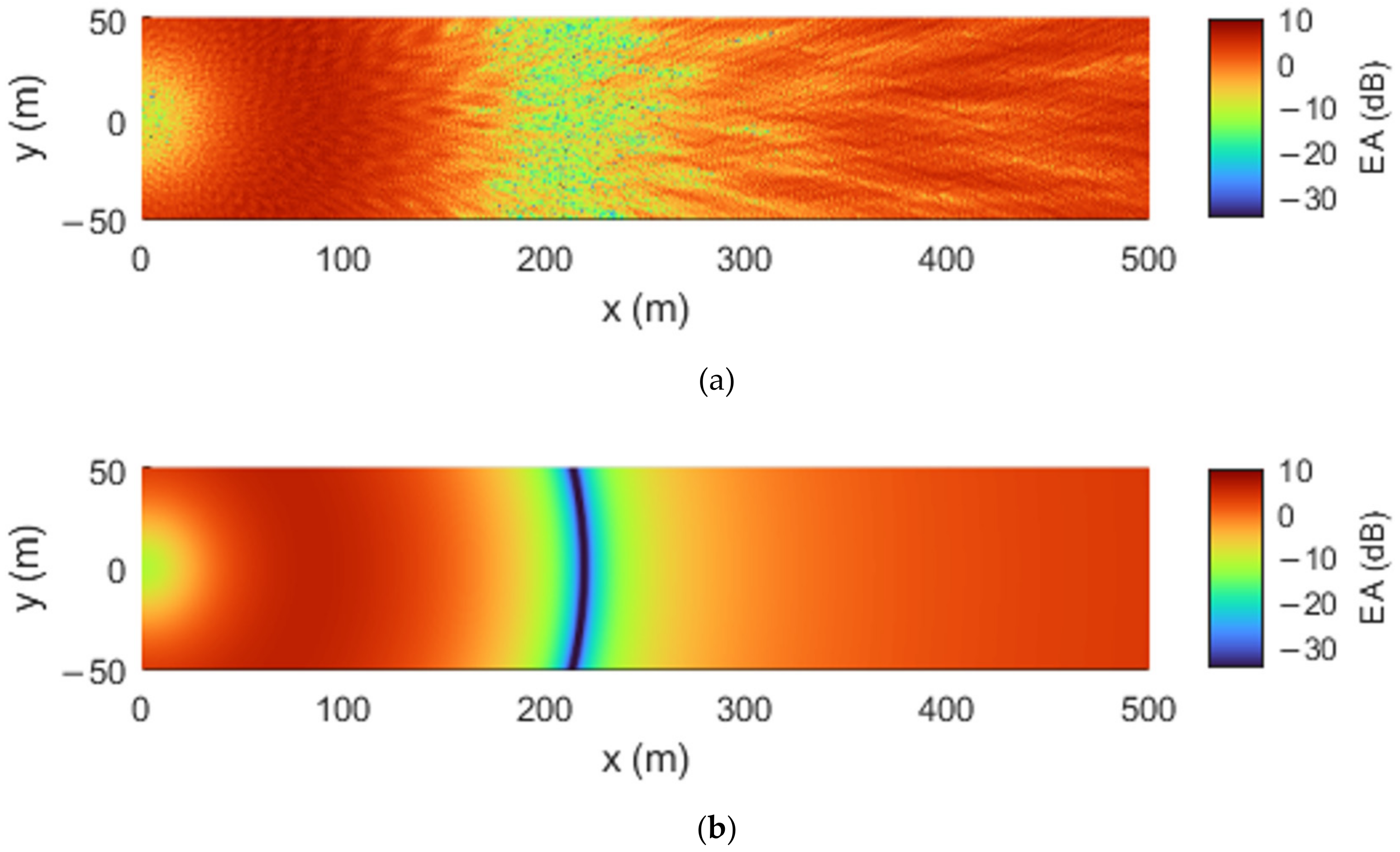
Conversely, in Figure 6, there are some major differences between the results from the flat ground and the rough ground. The ground interference dips, which are caused by destructive interference between the direct and reflected waves, are destroyed. This is not a novel result and is understood in the context of sound propagation over roughness. An interesting result is that the excess attenuation, in between the interference dips, highlights some significant reduction and amplification in sound pressure. Not including the ground interference dips, the excess attenuation at various points in the receiver plane at 125 Hz can differ from, but are not limited to, a range of ±3 dB. The same statement can be made for the 500 Hz case in Figure 7. Also, it is clear that, as the frequency increases, these patterns in the scattering effect become finer due, to some degree, to the decreased wavelength.

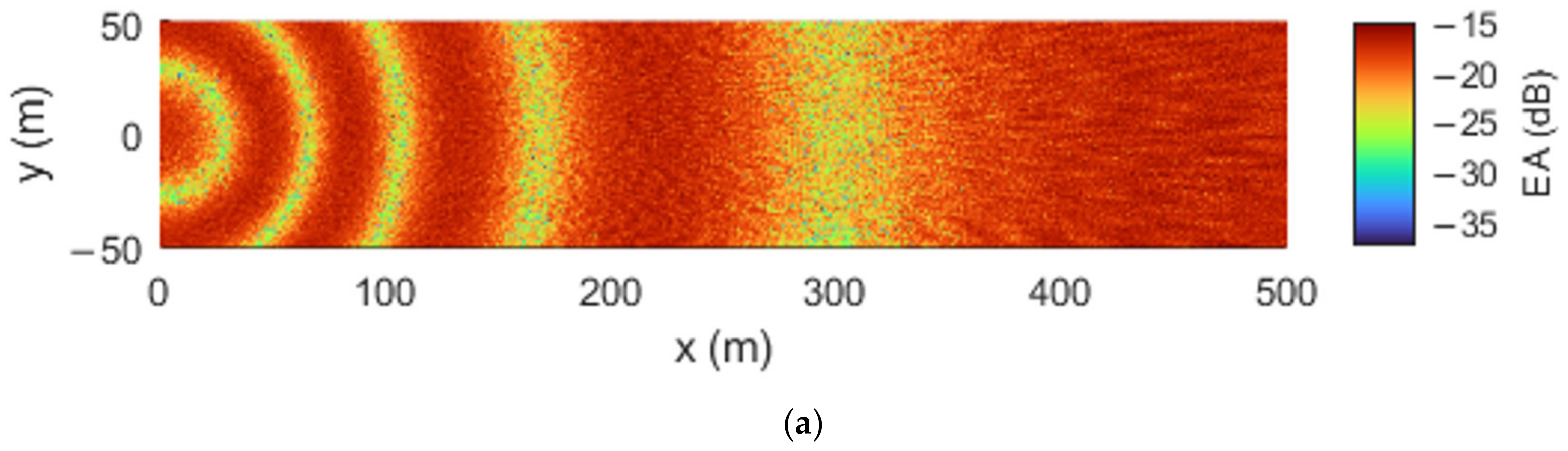
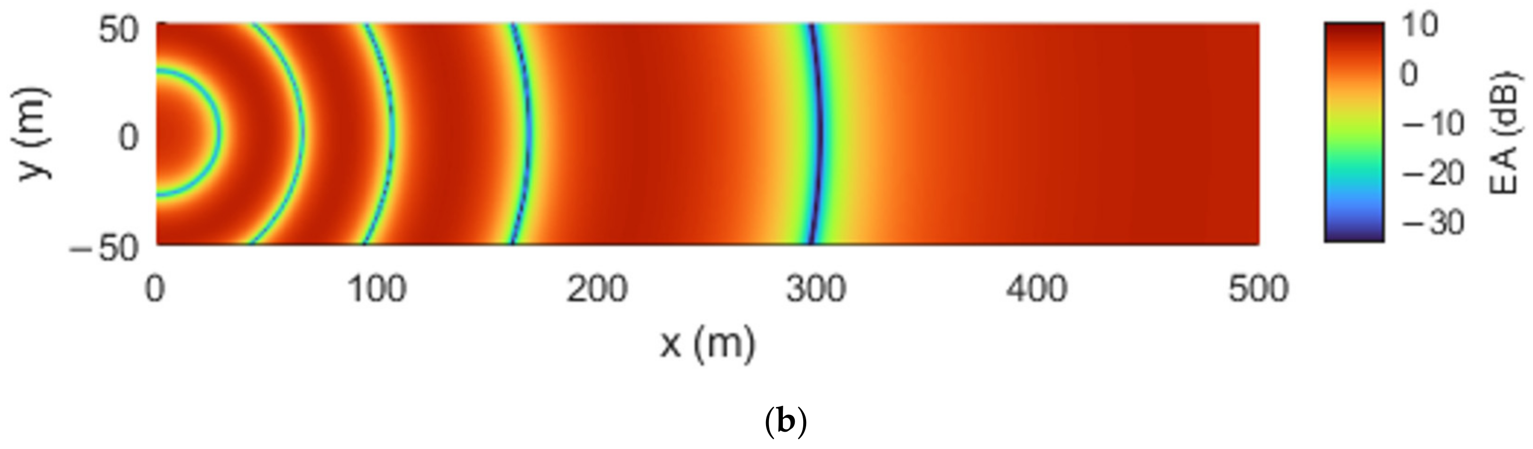
To highlight the significance of the scattering patterns, Figure 8 shows the excess attenuation plotted over a strip of receivers at 500 m of horizontal distance from the wind turbine sound source. Figure 8a shows the 63 Hz case while Figure 8b shows the 125 Hz case. Here, the sensitivity of the scattering effect to the frequency is clear. At lower frequencies, the is an overall reduction across the array of receivers, though the same cannot be said for the higher frequency case. As the frequency is increased, the scattering effect is amplified and the amplitude of the destructive and constructive interference patterns become more accentuated.

7. Discussion

The proposed MST was validated by comparison to experiment and numerical results, then applied towards predicting the reflection of wind turbine noise from a realistic rough ground, approximated by a distribution of hemispheres of various sizes. The results from the case study highlight significant fluctuations in the sound pressure level which is sensitive to the frequency under consideration. The reductions in the total sound pressure can be attributed to the interference effect caused by the non-specular reflections from the roughness. The results highlight a key point, namely that the scattering effect at relatively higher frequencies can both amplify and attenuate the sound pressure, and the magnitude of both appear to be dependent on the positioning of the receiver. Therefore, the scattering effect for a different source–receiver geometry may give entirely different results. This relationship between the roughness, the frequency, and the source–receiver geometry also raises the question of whether a roughness could be used practically for enhanced wind turbine noise reduction by arranging the hemispheres into patterns. Further work on both these questionings on source–receiver geometries and practical noise mitigation would be interesting.

Results from the validation of the proposed MST show that the theory can predict the reflected sound pressure up to the point where the wavelength is comparable to the hemisphere radius. This means it may be used for investigating higher frequency sound generated by wind turbines. Previous studies on wind turbine noise propagation over roughness were limited low frequencies since an effective impedance was used [45]. However, effective impedances are much quicker to compute than using a semi-analytical method like the proposed MST. An effective impedance is not the same as a multiple scattering theory and comparing the two critically can be challenging. Though, simply put, if low frequencies and small roughness is of interest, effective impedances may be a better choice. For example, an equivalent effective impedance for statistical distributions of hemispheres is given by Attenborough and Taherzadeh [46].

While the results outline the importance of a rough ground as a factor in wind turbine noise prediction, the discrepancy between the results using the approximated roughness (hemispheres) and a realistic roughness is unknown in context of the proposed MST. Chu and Stanton [47] compared results from a modified scattering theory from Twersky [48] (which was a scattering theory for hemispheres also) to measurements from a real rough surface to measurements from a real rough surface. They found that the agreement was reasonable. Though, for the proposed MST, further works on highlighting the accuracy of approximating a rough ground as a distribution of hemispheres would be reassuring.

While the proposed scattering theory is quite accurate, unfortunately the theory is not applicable when the reflecting plane is locally reacting, having a complex surface impedance. This is because the reflecting plane on which the hemispheres are placed must be sound hard for the image method to be used. If, however, the incident wave was assumed plane, which may be the case for studies on wind turbine noise, then theoretically a plane wave reflection coefficient may be attached to the reflected wave. Therefore, a locally reacting ground surface (e.g., most outdoor ground surfaces) may be considered. However, for spherical waves, we were not able to achieve such a formulation in this paper. Further works will aim to incorporate the acoustical properties of the ground by using a different approach in the theoretical formulations.

8. Conclusions

Formulations for a three-dimensional multiple scattering theory have been proposed in order to accurately predict the scattered pressure from a rough ground which has been approximated as a distribution of hemispheres of various radii. The theory has been validated against experimental and numerical results. The proposed theory was then applied to the unique source–receiver geometry of a wind turbine sound source and a human height receiver to highlight the significance of a rough ground effect on wind turbine noise propagation. Often, analyses of the roughness effect on wind turbine noise use effective impedance models to characterize the roughness effect [6,7,49]. However, this limits the analysis to roughness sizes and wavelengths where the scattering effect is mainly in the forward, specular direction. The proposed theory in this paper gives results that remain accurate up to the point where the radii of the hemispheres are comparable to the wavelengths of interest, which means that the scattering effect can be investigated more completely. The results from our case study have shown significant fluctuations in the excess attenuation over large distances from the wind turbine sound source, highlighting the possible influence of a ground roughness. The aim of the research is to shed light on the significance of a rough ground effect on sound propagation outdoors. We note that we chose a sound hard rough ground surface to isolate the scattering effect. Previous works on multiple scattering theories have heuristically used complex reflection coefficients to account for an absorbing ground plane [20,21], and future works may adopt this same treatment. Furthermore, it should be noted that the atmospheric effects were not incorporated into the proposed multiple scattering theory. This may be possible for weak refraction effects, where methods exist for replacing the radial path lengths by curves determined by the stratified atmosphere [11]. Incorporating these refraction effects is reserved for future works.