Article

Laboratory Validation of 3D Model and Investigating Its Application to Wind Turbine Noise Propagation over Rough Ground

The Acoustics Research Centre, The University of Hull, Hull HU6 7RX, UK
*
Author to whom correspondence should be addressed.
Wind 2024, 4(4), 363-375; https://doi.org/10.3390/wind4040018
Submission received: 6 September 2024 / Revised: 17 October 2024 / Accepted: 4 November 2024 / Published: 7 November 2024

Abstract

:
In an investigation into how wind turbine noise interacts with the surrounding terrain, its propagation over rough ground is simulated using a parabolic equation code using a modified effective impedance model, which characterizes the effects of a three-dimensional, rigid roughness within a relatively long wavelength limit ( k a 1 ). The model is validated by comparison to experiments conducted within an anechoic chamber wherein different source–receiver geometries are considered. The relative sound pressure level spectra from the parabolic equation code using the modified effective impedance model highlight a sensitivity to the roughness parameters. At a low frequency and far distance, the relative sound pressure level decreased as the roughness coverage increased. A difference of 4.9 dB has been reported. The simulations highlight how the roughness shifts the ground effect dips, resulting in the sound level at the distance of 2 km being altered. However, only the monochromatic wave has been discussed. Further work on broadband noise is desirable. Furthermore, due to the long wavelength limit, only a portion of audible wind turbine noise can be investigated.

1. Introduction

Large wind turbines are quite serious sources of noise, making the acoustic impact one of the major hindrances to the public’s acceptance of the technology [1,2]. Conclusions from a government-commissioned analysis of the current guidance for wind turbine noise control in the UK indicate that the current framework [3] is outdated in light of the large volume of new research and technologies spanning decades after the initial publishing of the document [4].
Reviews on the effects of wind turbine noise indicate that, at a minimum, wind turbine noise is a cause for annoyance, and despite the levels being modest compared to other sources like traffic noise, the wind turbine noise seems more annoying [5].
This paper focuses on the reflections and scattering of the noise from the rough terrain that often surrounds wind turbines. It is well understood that roughness can have a significant effect on the propagation of sound, such that considering its effect in the context of wind turbine noise is worthwhile. It is valuable to understand how this noise propagates through the environment toward the homes of those living near wind turbines to improve the micrositing process and minimize the environmental impact.
Much effort devoted to researching the roughness effect on noise propagation has illuminated the advantages and disadvantages of the various available methods. Some authors have utilized the roughness directly, incorporating the surface roughness profile in their numerical calculations [6,7]. However, under certain circumstances, the roughness can be assumed to be an intrinsic property of the ground surface. Under this assumption, the rough surface can be thought of as a flat one with modified acoustic properties (modified impedance). In this case, the modified acoustic property is called an effective impedance, Z e f f [8,9,10]. This method has also been applied to the numerical simulation of wind turbine noise and other noise sources over a rough sea surface by considering the sea wave velocity as being much smaller than the speed of sound such that the sea roughness can be considered static [11,12]. Compared to directly incorporating a rough surface profile in the simulation of the sound propagation, the effective impedance approach is computationally more efficient and simpler to apply.
Effective impedances have been used extensively in studies on the propagation of wind turbine noise over a rough surface [12,13,14]. However, not yet has a three-dimensional roughness been employed; only two-dimensional effective impedance models have been of interest. Therefore, in this paper, a three-dimensional effective impedance model will be chosen and validated for its use in the simulation of wind turbine noise propagation. Then, said effective impedance model will be used to investigate the propagation of wind turbine noise over large distances of rough terrain, discussing its significance in its effect on the perceived noise levels.

2. Methods

2.1. Effective Impedance Model

Some of the first works on the subject of effective impedances can be attributed to Twersky’s work [15]. In this work, a theory for the scattered field above a flat surface cluttered with semicylinders and/or hemispheres was derived. The scattered field was a function of the statistical distribution of the scatterers as well as of their individual scattering behavior. From the theory, approximations for the reflection coefficients could be calculated. Later, the theory was used to create boundary conditions for the rough surface [16,17]. These boundary conditions, in turn, were then extended with an emphasis on the scatterer shape [18]. The extended boundary conditions were then used to derive an effective impedance for a planar distribution of arbitrary three-dimensional scatterers [9]. However, to maintain that the roughness effects are solely an intrinsic property of the ground surface, these models are restricted to cases where the wavelengths are large relative to the roughness size. In such cases, the scattering is mainly in the forward, specular direction [19]. This limit is given by k a 1 , where k and a are the wavenumber and the height of the roughness, respectively. Resultingly, effective impedance models are sometimes called long wavelength approximations. Further literature on the topic can be found in Ogilvy [20].
In this paper, a rough surface is idealized by 0.0135 m radius polyurethane hemispheres distributed across a smooth Perspex sheet. The hemispheres were chosen to represent hills using a simple, canonical shape. Therefore, the impedance model to be used must suit the roughness type in mind. An effective impedance model, which will be called the Attenborough–Tolstoy effective impedance model, accommodates such a roughness. Consider a reflecting plane with density, ρ 3 ( k g / m 3 ), and sound speed, c 3 ( m / s ), on which a distribution of the hemispherical scattering elements lies. The hemispheres have density, ρ 2 , sound speed, c 2 , radius, a (m), and a mean center-to-center spacing, L (m). L is a parameter concerning the interaction between scattering objects.
The atmosphere above the reflecting plane and the scattering objects then has a density ρ 1 and sound speed c 1 . The model can be modified when ρ 3 ρ 1 and ρ 2 ρ 1 such that the hemisphere density is assumed to be much larger than the atmospheric density. The equation for the effective admittance (inverse of impedance) is then given by
β e f f = 1 Z e f f = i k σ V 3 2 s 3 1 + 3 π σ V s 3 8 N L 3 1 1
N is the number of hemispheres per m2, σ V is the volume occupied by the hemispheres per m2  2 3 N π a 3 , s 3 is a shape factor (equal to 1 for hemispheres), k is the wavenumber, and i = 1 . By making the assumptions on the densities of the scatterers, Equation (1) is a modified version of the Attenborough–Tolstoy effective impedance model. However, the model is still restricted to wavelengths that are larger than the roughness size. This limit will be discussed in a later section. Note that in this modified effective impedance model, the real part of the effective impedance goes to zero, indicating that the small absorption that would be attributed to the scatterers is neglected.
Various distributions of 0.0135 m radius polyurethane hemispheres are placed on the Perspex sheet. The parameters characterizing the distribution include the number of hemispheres per unit area, N, and the mean center-to-center spacing between the hemispheres, L (m). L is calculated as the mean length between the center of each scattering element and the 8 immediate scattering elements nearby. Calculating the mean spacing using the distances between more elements gives similar enough values of L to neglect them. However, it is more intuitive to characterize the roughness by the percentage coverage per unit area, n (%). For N = 1372 , the mean center-to-center spacing was 0.033 m, and the percentage coverage was 78.5%. Table 1 shows the details for all the roughness types. Figure 1 then shows a diagram of the roughness distributions.
Figure 2 shows the predicted normalized effective impedances for the various roughness types using the modified model (Equation (1)). Only the imaginary part is shown since Equation (1) denotes a solely imaginary part of the effective impedance (reactance) for the solid acoustic rigid surface.

2.2. Sound Field Above a Locally Reacting Ground

When the effective admittance is calculated, it can be incorporated into the analytical theory for the sound field above a locally reacting ground. Consider the geometry of a sound source at ( 0 , 0 , z s ) and a receiver at r = ( x , y , z ) with a reflecting plane at z = 0 . With time dependence suppressed, the pressure at the receiver p r can be calculated [21].
p r = e x p i k r 1 4 π r 1 + R p + 1 R p F w e x p i k r 2 4 π r 2
r 1 is the distance between the source and the receiver, while r 2 is the distance from the image source ( 0 , 0 , z s ) to the receiver. R p is the plane wave reflection coefficient, and F w is often called the boundary loss factor.
R p = cos θ β cos θ + β
F w = 1 + i π w e x p w 2 e r f c i w
θ is the angle made between the incident wave vector and the axis normal to the reflecting plane. e r f c is a complimentary error function that can be approximated [22]. Finally, w is called the numerical distance.
w = 1 2 1 + i k r 2 cos θ + β
The admittance, β , is then substituted for the effective admittance calculated using the modified Attenborough–Tolstoy model in Equation (1).

2.3. Principles of Parabolic Equation (PE) Method

The parabolic equation method [23] allows fast prediction of noise levels over large distances in an inhomogeneous atmosphere. Because wind speed and sound speed gradients can be incorporated, the method is a popular tool for predicting wind turbine noise. Comparisons between the PE method and measurements from existing wind turbines have shown its effectiveness [24].
The propagation method in this paper is a wide-angle parabolic equation method solved using the Crank-Nicholson finite difference scheme [25]. The method assumes propagation in an inhomogeneous medium, though, for simplicity, a homogeneous atmosphere (constant sound speed, c ) can be chosen. The sound field is governed by the following Helmholtz equation.
2 x 2 + 2 z 2 + k 2 Ψ x , z = 0
k is the wavenumber at altitude z, and Ψ ( x , z ) is a complex quantity related to the acoustic pressure by p x , z = Ψ ( x , z ) / x . x and z denote the horizontal range and vertical height, respectively. An operator, q , is introduced.
q = 1 k 0 2 2 z 2 + k 2 1
k 0 is a reference sound speed, k 0 = ω / c 0 . Considering the operator, q , and only considering outgoing waves, the Helmholtz equation reduces to
x i k 0 1 + q Ψ x , z = 0
for which a solution is chosen.
Ψ x , z = φ x , z exp i k 0 x
In the proposed solution, exp ( i k 0 x ) is the carrier function, and φ x , z is a slowly varying envelope function. A second-order accurate approximation for 1 + q is then introduced.
1 + q 1 + 3 q 4 1 + q 4
This approximation allows Equation (9) to be written as
1 + q 4 Ψ x = i k 0 1 + 3 q 4 Ψ
from which the corresponding equation for the envelope function, φ , is
1 + q 4 φ x = i k 0 q 2 φ
This is the key principle of the wide-angle parabolic equation method. Equation (12) is solved over a vertical strip of the atmosphere given by grid points, z j = j z for j = 1 , 2 , , M and is then marched horizontally by grid points, x i = i x for i = 1 , 2 , , N . From a convergence test, it is found that it is best practice to have a grid step size, Δ x = λ / 10 and Δ z = λ / 10 where λ is the wavelength of interest. For the ground boundary conditions, an impedance boundary condition is given. This is where the effective impedance, Equation (1), is incorporated. The roughness effect is considered a property of the ground and is not a function of the source–receiver geometry and/or refraction effects. The PE code is implemented in MATLAB.

2.4. Experiment Methods

In an anechoic chamber, a speaker fitted with a copper pipe was placed at 100 mm above a 1 m × 1 m Perspex sheet. The inner diameter of the copper pipe which was attached to the speaker was 20 mm. The purpose of the pipe was to reduce reflections from the source and the apparatus holding it in place. This also ensured the sound source was a point source. A 1/2-inch Bruel & Kjaer (Nærum, Denmark) condenser microphone was then placed 100 mm above the Perspex sheet. The horizontal distance between the speaker and microphone was 400 mm. For each distribution of hemispheres, 50 measurements were taken.
Further measurements were then taken, which employed a lower receiver. The sound source and the receiver were placed at 200 mm and 20 mm, respectively, above the Perspex sheet. The horizontal distance between the two was 100 mm. Only the closely packed roughness is considered in this case. For the latter set of measurements, they will be called situation 1 and for the former, they will be called situation 2. An analysis of the ray paths ensured the boundaries of the experiment site would not cause interference.
An RS PRO RSDG830 Series Waveform Generator fed successively to a Sony (Tokyo, Japan) Signal Amplifier, then to the speaker, was used to produce acoustic impulses. Impulse signals were used as they can show the effects of a scattered field more clearly. Next, a 1/2-inch Brüel & Kjaer condenser microphone, fed successively to a Brüel & Kjaer Amplifier and then to a National Instruments 5911 Series Data Acquisition Card, was used to save the data on a National Instruments (Austin, TX, USA) LABVIEW virtual oscilloscope software (version 2.1). Figure 3 shows a diagram of the apparatus arrangement.

3. Results

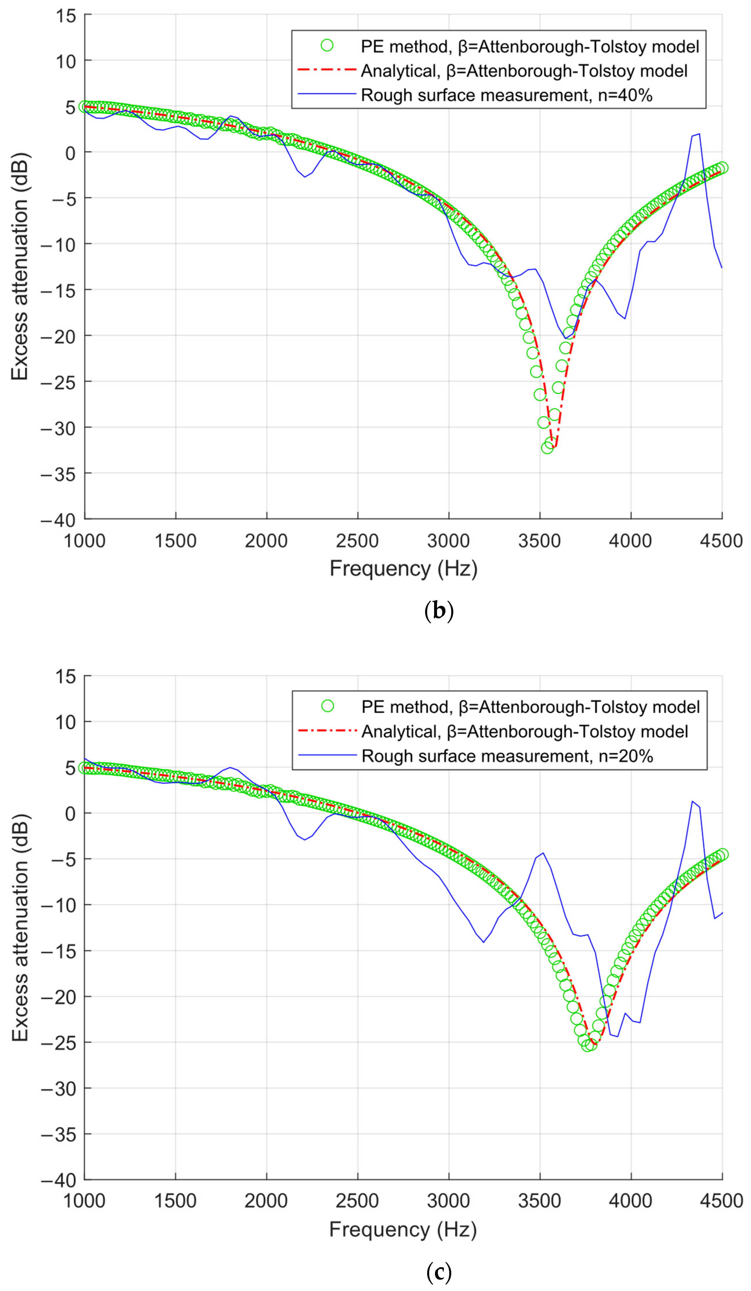
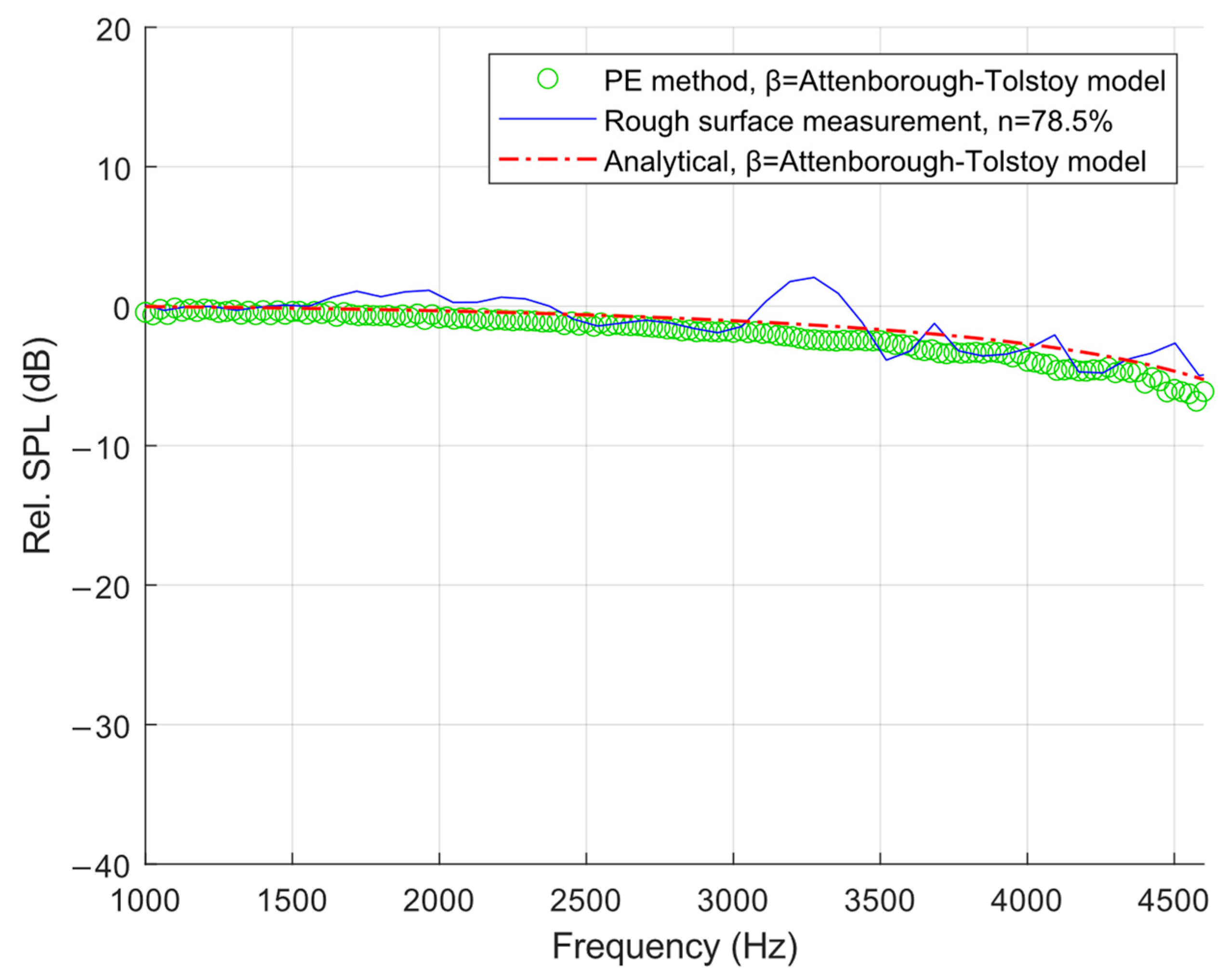
3.1. Validation of the Effective Impedance Model

The recorded time domain data were used to calculate the attenuation of sound pressure in excess of the direct field, called excess attenuation, E A , in d B .
E A d B = 10 log 10 P 2 / P r e f 2
P is the total acoustic pressure (direct, reflected, and scattered) and P r e f is the direct field pressure from the source to the receiver. The reference pressure is measured by maintaining the direct distance between the source and receiver but removing the ground boundary by adjusting the height of the source and receiver to a relatively large distance above the ground such that reflection may not be recorded. The recorded time domain data is transferred to the frequency domain using a Fourier transform algorithm. So, the pressures, P and P r e f , are evaluated over their frequency spectra. For each roughness type, after signals are transferred to the frequency domain and the excess attenuation is calculated, the average excess attenuation is reported.
Figure 4 shows the comparisons of the measured excess attenuation to that predicted by the analytical and the parabolic equation theory. The analytical and parabolic equation theory both use an effective impedance calculated from Equation (1). In the parabolic equation simulations, to remain consistent with the experiment methods, a starting function was used to represent a point source [26]. Furthermore, the grid spacing was 0.001 m. Because the effective impedance model assumes the roughness is an intrinsic property of flat ground, it was also necessary to shift the reflecting plane upwards slightly in the calculations (by roughly 1/2 of the hemisphere radius).
The Attenborough–Tolstoy effective impedance model shows the shift in the ground effect dips, which are a consequence of the rough surface, to a tolerable accuracy. Since the model only gives an imaginary part of the impedance, the reactance and phase shifts are the only roughness effects expected anyway. It is also clear to see the discrepancies as the relatively large wavelength limit ( k a 1 ) is strained. However, within the limit, there is little discrepancy.
The large negative excess attenuation can be attributed to the destructive interference between the directly received sound wave and that which is reflected from the slightly rough ground. Roughness can alter the phase of a reflected wave, which can significantly shift interference effects to a different frequency [27].
Regarding the experiments that employed a relatively low receiver, the attenuation in excess of the direct field was not calculated. Rather, the attenuation was calculated with reference to the total pressure taken over a smooth, rigid ground with the same source–receiver geometry. This method isolated the roughness effect. The attenuation with reference to the smooth, rigid ground is given by R e l . S P L (for Relative Sound Pressure Level) because the term excess attenuation is generally reserved for the attenuation in excess of a direct field.
R e l . S P L d B = 10 log 10 P r o u g h 2 / P s m o o t h 2
P r o u g h is the total acoustic pressure (direct, reflected and scattered) from the measurements taken under a rough ground condition, P s m o o t h is the total acoustic pressure (direct and reflected) taken under a smooth ground condition. Figure 5 shows the comparisons of the measured relative sound pressure level to that predicted by the analytical and parabolic equation theory. In the case of the unique source–receiver geometry, the ground effects may shift at much higher frequencies where the impedance model limit is exceeded. Nevertheless, the curves of the measured data and the theory are consistent.

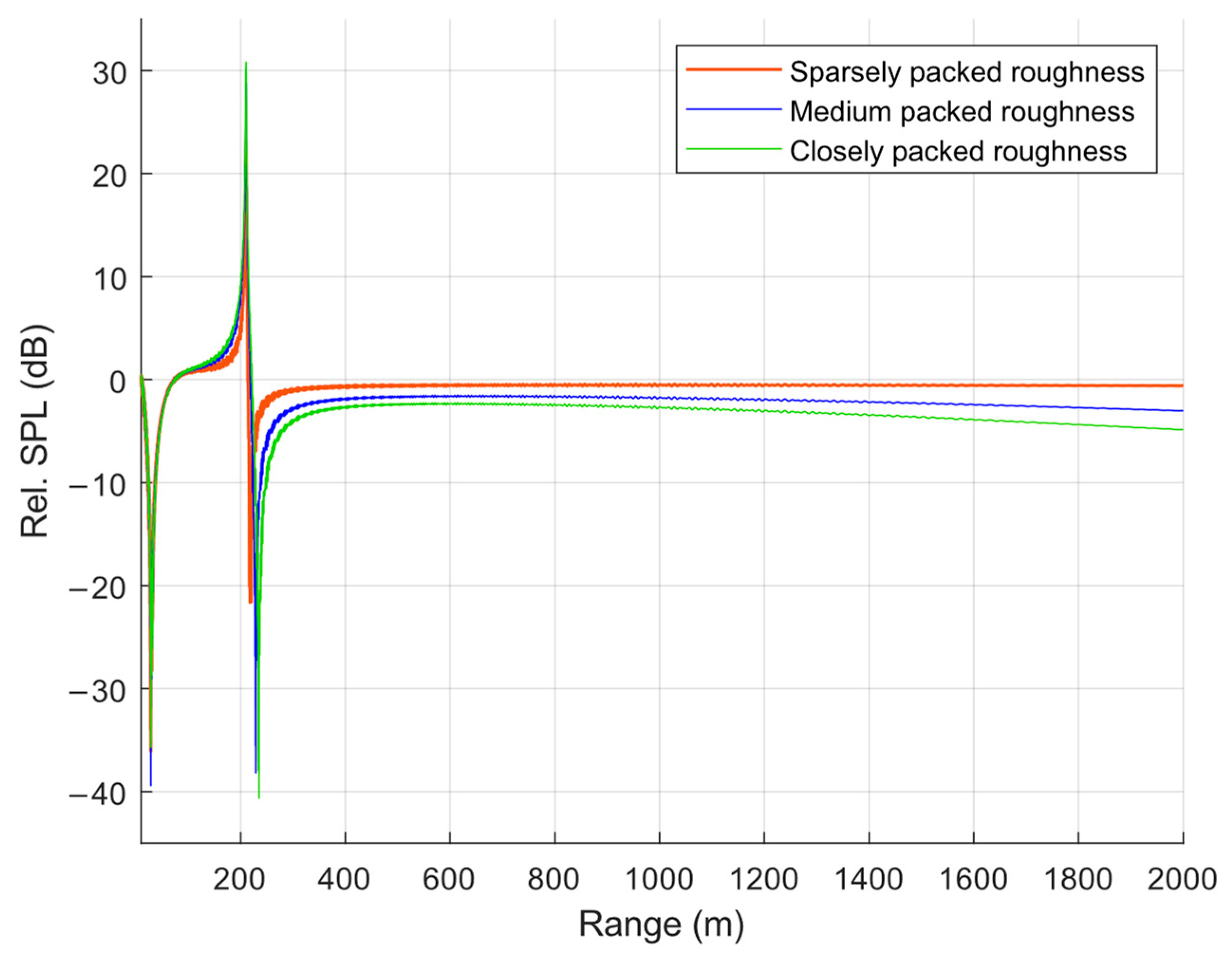
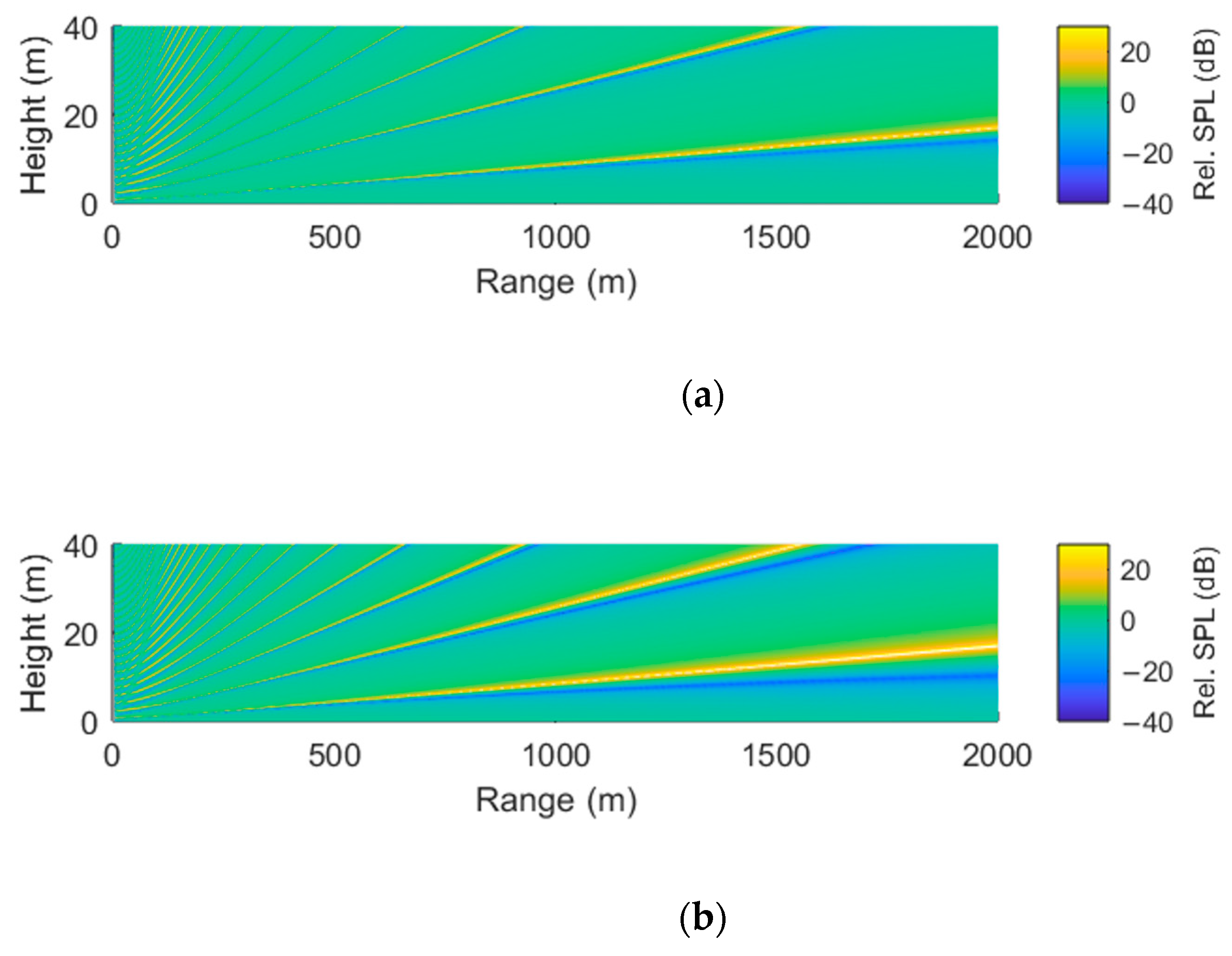
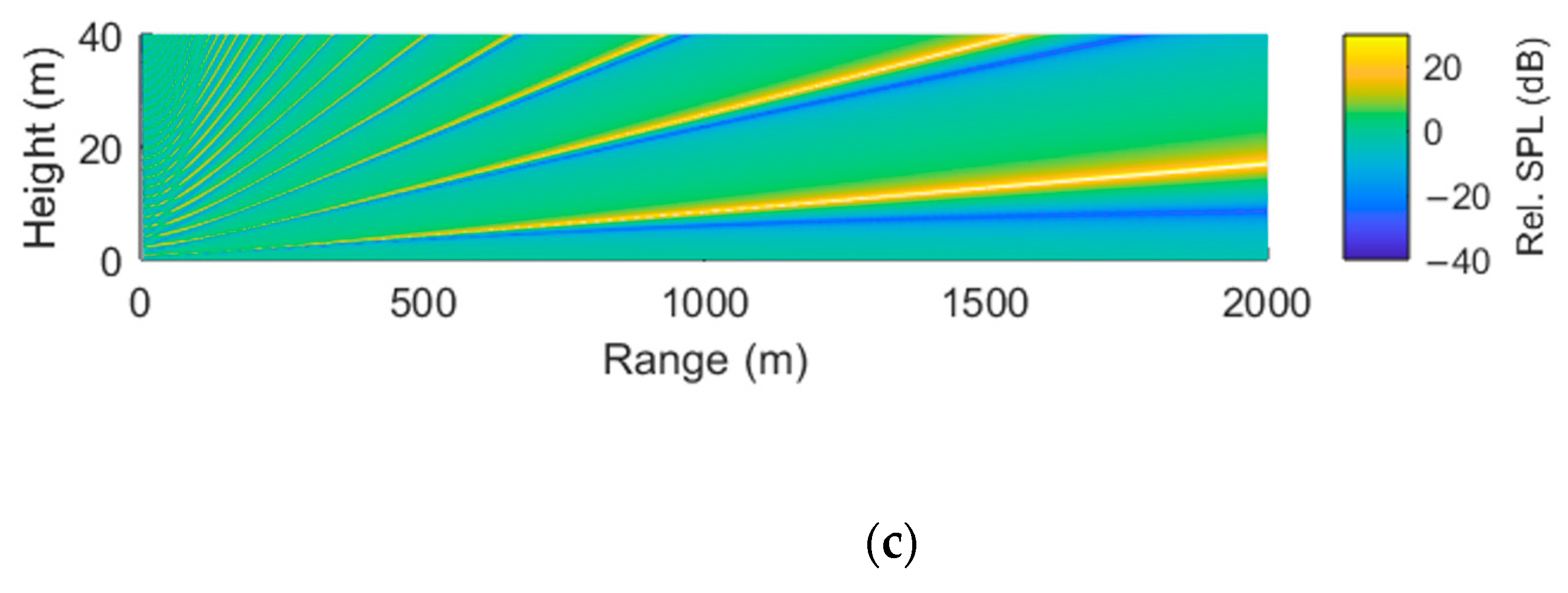
3.2. Further Parabolic Equation Method Simulations

Since the effective impedance model gave results consistent with the measured experiment data, further PE simulations using the model were conducted. To represent a wind turbine, the sound source was taken as a point source located at the center of the wind turbine nacelle at 100 m above the ground. Regarding the noise source, some authors use three-point sources [7,24,28,29,30]. The locations of these point sources are taken from studies on the localization of wind turbine noise sources [31]. However, as propagation distance increases into the far field ( k r 1 ), the point source approximation becomes valid for representing a wind turbine [28]. Furthermore, a point source is chosen to remain consistent with the previous parabolic equation simulations. The receiver was taken at 2 m to represent the human perception of wind turbine noise, and the ground roughness was given by various distributions of 0.2 m radius hemispherical bosses. The roughness may represent rough ground, which can be idealized by hemispherical bosses. Figure 6 shows a diagram of the scenario in mind.
A frequency of 100 Hz was chosen. Low-frequency noise still remains within the spectrum of wind turbine noise, though not dominant [32]. Therefore, studying these frequencies is still valuable and the limit will be discussed in a later section. The grid sizing was given by Δ x = z = 0.2 m . The distributions of the hills are characterized by their number per unit area, N, which ranged between 6 for a closely packed roughness density, 3 for a medium-packed roughness density and 1 for a sparsely packed roughness density. The same distributions as in Figure 1 were used. Further details on the roughness are found in Table 2.
The parameters of the roughness were used to determine the corresponding effective impedance using Equation (1). The relative sound pressure level, Equation (14), was calculated to emphasize the roughness effect alone. Figure 7 shows the predicted relative sound pressure levels.
The results at 2 km vary significantly with the roughness type. The values of the relative sound pressure levels at 2 km are reported in Table 3. Figure 8 shows the roughness effect across the domain close to the ground, which becomes more prominent as the roughness coverage increases. The effect in Figure 7 can be seen in Figure 8.

4. Discussion

The modified Attenborough–Tolstoy effective impedance model showed the shift in the ground effect dips to tolerable accuracy within the relatively long wavelength limit. Since the model only gives an imaginary part of the effective impedance, phase shifts are the only roughness effect expected.
When the experimental apparatus was altered to a high source and a low receiver, the curves from the theory fitted well with the measured data, too. However, no ground effect dips were measured. Furthermore, it was necessary to lift the reflecting plane in the theory by one-half the radius of the hemispheres to give the most accurate results. This follows since the effective impedance idealizes the rough surface as a smooth one. So, intuitively, the level of this smooth surface would be between the maximum and minimum heights of the roughness.
Regarding the relatively long wavelength limit, not always will it be the case that the wavelength is large compared to the roughness size. When the wavelength approaches the roughness size (or vice versa), scattering in random, non-specular directions dominates [19,33]. Therefore, the roughness effect cannot be treated simply by an effective impedance. A non-specular, randomly scattered field depends on, for example, source–receiver geometry and the refraction effects [6]. All these factors are pertinent to wind turbine noise. Therefore, treating a rough ground with an effective impedance may not be suitable in all cases. The effects of scattering at higher frequencies are expected to be more significant than at low frequencies for these PE simulations. Therefore, treating a rough ground with an effective impedance may not be suitable in all cases. Furthermore, especially when larger roughness or higher frequencies are considered, a large portion of audible wind turbine noise is excluded by the model (the trailing edge noise, for instance). Therefore, it is appropriate to discuss alternative approaches and possible further work.
For example, the use of a generalized terrain parabolic equation is more computationally demanding but will simulate non-specular scatter in a one-way propagation scheme [34].
In regard to the effect of the actual surface roughness of each of the hemispherical bosses, for a surface roughness that is at such small a scale compared to the size of the hemisphere, any scattering effects are expected at much higher frequencies where the wavelengths are comparable to the surface roughness. Therefore, for the frequencies of interest, the effects of the roughness of the scatterer surface can be neglected.
Furthermore, in the derivation of the Attenborough–Tolstoy effective impedance model, the second-order derivatives in the boundary conditions are ignored. These components of the boundary conditions account for the dipole contributions, which may have a significant effect on the perception of wind turbine noise from a person’s perspective. Further works may investigate the significance of the contribution.
Concerning the further parabolic equation method simulations, the predicted relative sound pressure levels highlighted a clear sensitivity to the roughness parameters. At a low frequency and far distance, the relative sound pressure level decreased as the roughness coverage increased. A difference of 4.9 dB has been reported. In the context of the noise restrictions imposed on wind farm projects, a difference of 4.9 dB can certainly alter the micrositing process and the position of a wind turbine.
It is important to note also that the roughness considered is not necessarily truly representative of real, random ground topography. Therefore, the discrepancy between the effects of the idealized roughness and the realistic roughness is understood. However, comparisons between Twersky’s theory [15] for the scattering from bosses (from which the effective impedance model originates) and measurements from a random roughness have shown reasonable agreement [35].

5. Conclusions

An effective impedance model for a three-dimensional roughness has been modified and validated for its use in simulating wind turbine noise over rough ground by comparison to results from experiments in an anechoic chamber. The effective impedance model was then used in conjunction with the parabolic equation theory to simulate the propagation of wind turbine noise over large distances of roughness. Results highlight a clear sensitivity to the roughness parameters. At a low frequency and far distance, the relative sound pressure level decreased as the roughness coverage increased. A difference of 4.9 dB has been reported. Further work might investigate a more general roughness profile as well as the roughness caused by sea waves in the context of offshore wind turbine noise. Due to the high impedance of water, the sea wave roughness can be treated as hard, and a similar effective impedance approach may be taken.

Author Contributions

Conceptualization, J.N. and Q.Q.; methodology, J.N. and Q.Q.; software, J.N.; validation, Q.Q. and J.N.; formal analysis, J.N.; investigation, J.N. and Q.Q.; resources, J.N. and Q.Q.; data curation, J.N.; writing—original draft preparation, J.N.; writing—review and editing, Q.Q. All authors have read and agreed to the published version of the manuscript.

Funding

This research received no external funding.

Institutional Review Board Statement

Not applicable.

Informed Consent Statement

Not applicable.

Data Availability Statement

The raw data supporting the conclusions of this article will be made available by the authors on request.

Conflicts of Interest

The authors declare no conflicts of interest.

References

  1. van den Berg, F. A Proposal to Use Determinants of Annoyance in Wind Farm Planning and Management. Wind 2022, 2, 571–585. [Google Scholar] [CrossRef]
  2. da Silva, V.P.; Galvão, M.L.D.M. Onshore wind power generation and sustainability challenges in Northeast Brazil: A quick scoping review. Wind 2022, 2, 192–209. [Google Scholar] [CrossRef]
  3. Working Group on Noise from Wind Turbines; ETSU. The Assessment and Rating of Noise from Wind Farms; Easte Tennessess State University: Johnson City, TN, USA, 1996. [Google Scholar]
  4. Lotinga, M.; Lewis, T.; Powlson, J.; Berry, B. Onshore wind turbine noise: A review of the current guidance framework for the UK Government (Part 2: Conclusions and recommendations). Acoust. Bull. 2023, 49, 26–38. [Google Scholar]
  5. van Kamp, I.; van den Berg, F. Health effects related to wind turbine sound: An update. Int. J. Environ. Res. Public Health 2021, 18, 9133. [Google Scholar] [CrossRef] [PubMed]
  6. Vecchiotti, A.; Ryan, T.J.; Vignola, J.F.; Turo, D. Atmospheric Sound Propagation over Rough Sea: Numerical Evaluation of Equivalent Acoustic Impedance of Varying Sea States. Acoustics 2024, 6, 489–508. [Google Scholar] [CrossRef]
  7. Shen, W.Z.; Zhu, W.J.; Barlas, E.; Li, Y. Advanced flow and noise simulation method for wind farm assessment in complex terrain. Renew. Energy 2019, 143, 1812–1825. [Google Scholar] [CrossRef]
  8. Boulanger, P.; Attenborough, K.; Taherzadeh, S.; Waters-Fuller, T.; Li, K.M. Ground effect over hard rough surfaces. J. Acoust. Soc. Am. 1998, 104, 1474–1482. [Google Scholar] [CrossRef]
  9. Attenborough, K.; Taherzadeh, S. Propagation from a point source over a rough finite impedance boundary. J. Acoust. Soc. Am. 1995, 98, 1717–1722. [Google Scholar] [CrossRef]
  10. Brelet, Y.; Bourlier, C. SPM numerical results from an effective surface impedance for a one-dimensional perfectly-conducting rough sea surface. Prog. Electromagn. Res. 2008, 81, 413–436. [Google Scholar] [CrossRef]
  11. Boulanger, P.; Attenborough, K. Effective impedance spectra for predicting rough sea effects on atmospheric impulsive sounds. J. Acoust. Soc. Am. 2005, 117, 751–762. [Google Scholar] [CrossRef]
  12. Johansson, L. Sound Propagation Around Off-Shore Wind Turbines; Byggvetenskap: Stockholm, Sweden, 2003. [Google Scholar]
  13. Van Renterghem, T.; Botteldooren, D.; Dekoninck, L. Airborne sound propagation over sea during offshore wind farm piling. J. Acoust. Soc. Am. 2014, 135, 599–609. [Google Scholar] [CrossRef] [PubMed]
  14. Kayser, B.; Gauvreau, B.; Ecotière, D. Sensitivity analysis of a parabolic equation model to ground impedance and surface roughness for wind turbine noise. J. Acoust. Soc. Am. 2019, 146, 3222–3231. [Google Scholar] [CrossRef]
  15. Twersky, V. On scattering and reflection of sound by rough surfaces. J. Acoust. Soc. Am. 1957, 29, 209–225. [Google Scholar] [CrossRef]
  16. Biot, M.A. Reflection on a rough surface from an acoustic point source. J. Acoust. Soc. Am. 1957, 29, 1193–1200. [Google Scholar] [CrossRef]
  17. Biot, M.A. Generalized boundary condition for multiple scatter in acoustic reflection. J. Acoust. Soc. Am. 1968, 44, 1616–1622. [Google Scholar] [CrossRef]
  18. Tolstoy, I. Coherent sound scatter from a rough interface between arbitrary fluids with particular reference to roughness element shapes and corrugated surfaces. J. Acoust. Soc. Am. 1982, 72, 960–972. [Google Scholar] [CrossRef]
  19. Brekhovskikh, L. Diffraction of waves on an uneven surface, 2(Diffraction of acoustic and electromagnetic waves on wavy surfaces). Zh. Eksperim. Teor. Fiz. 1952, 23, 289–304. [Google Scholar]
  20. Ogilvy, J. Wave scattering from rough surfaces. Rep. Prog. Phys. 1987, 50, 1553. [Google Scholar] [CrossRef]
  21. Attenborough, K.; Van Renterghem, T. Predicting Outdoor Sound; CRC Press: Boca Raton, FL, USA, 2021. [Google Scholar]
  22. Abramowitz, M.; Stegun, I.A. Handbook of Mathematical Functions with Formulas, Graphs, and Mathematical Tables; United States Government Printing Office: Washington, DC, USA, 1948; Volume 55. [Google Scholar]
  23. Tappert, F.D. The parabolic approximation method. In Wave Propagation and Underwater Acoustics; Springer: Berlin/Heidelberg, Germany, 2005; pp. 224–287. [Google Scholar]
  24. Könecke, S.; Hörmeyer, J.; Bohne, T.; Rolfes, R. A new base of wind turbine noise measurement data and its application for a systematic validation of sound propagation models. Wind. Energy Sci. Discuss. 2022, 8, 639–659. [Google Scholar] [CrossRef]
  25. West, M.; Gilbert, K.; Sack, R. A tutorial on the parabolic equation (PE) model used for long range sound propagation in the atmosphere. Appl. Acoust. 1992, 37, 31–49. [Google Scholar] [CrossRef]
  26. Salomons, E.M. Computational Atmospheric Acoustics; Springer Science & Business Media: Berlin/Heidelberg, Germany, 2001. [Google Scholar]
  27. Bashir, I.; Taherzadeh, S.; Attenborough, K. Diffraction assisted rough ground effect: Models and data. J. Acoust. Soc. Am. 2013, 133, 1281–1292. [Google Scholar] [CrossRef] [PubMed]
  28. Nyborg, C.; Fischer, A.; Thysell, E.; Feng, J.; Søndergaard, L.S.; Sørensen, T.; Hansen, T.R.; Hansen, K.S.; Bertagnolio, F. Propagation of wind turbine noise: Measurements and model evaluation. J. Phys. Conf. Ser. 2022, 2265, 032041. [Google Scholar] [CrossRef]
  29. Ecotière, D. Can we really predict wind turbine noise with only one pointsource. In Proceedings of the 6th International Meeting on Wind Turbine Noise, Glasgow, Scotland, 20–23 April 2015. [Google Scholar]
  30. Barlas, E.; Zhu, W.J.; Shen, W.Z.; Dag, K.O.; Moriarty, P. Consistent modelling of wind turbine noise propagation from source to receiver. J. Acoust. Soc. Am. 2017, 142, 3297–3310. [Google Scholar] [CrossRef] [PubMed]
  31. Oerlemans, S.; Sijtsma, P.; López, B.M. Location and quantification of noise sources on a wind turbine. J. Sound Vib. 2007, 299, 869–883. [Google Scholar] [CrossRef]
  32. Søndergaard, B. Low frequency noise from wind turbines: Do the Danish regulations have any impact? An analysis of noise measurements. Int. J. Aeroacoust. 2015, 14, 909–915. [Google Scholar] [CrossRef]
  33. Eckart, C. The scattering of sound from the sea surface. J. Acoust. Soc. Am. 1953, 25, 566–570. [Google Scholar] [CrossRef]
  34. Sack, R.; West, M. A parabolic equation for sound propagation in two dimensions over any smooth terrain profile: The generalised terrain parabolic equation (GT-PE). Appl. Acoust. 1995, 45, 113–129. [Google Scholar] [CrossRef]
  35. Chu, D.; Stanton, T. Application of Twersky’s boss scattering theory to laboratory measurements of sound scattered by a rough surface. J. Acoust. Soc. Am. 1990, 87, 1557–1568. [Google Scholar] [CrossRef]
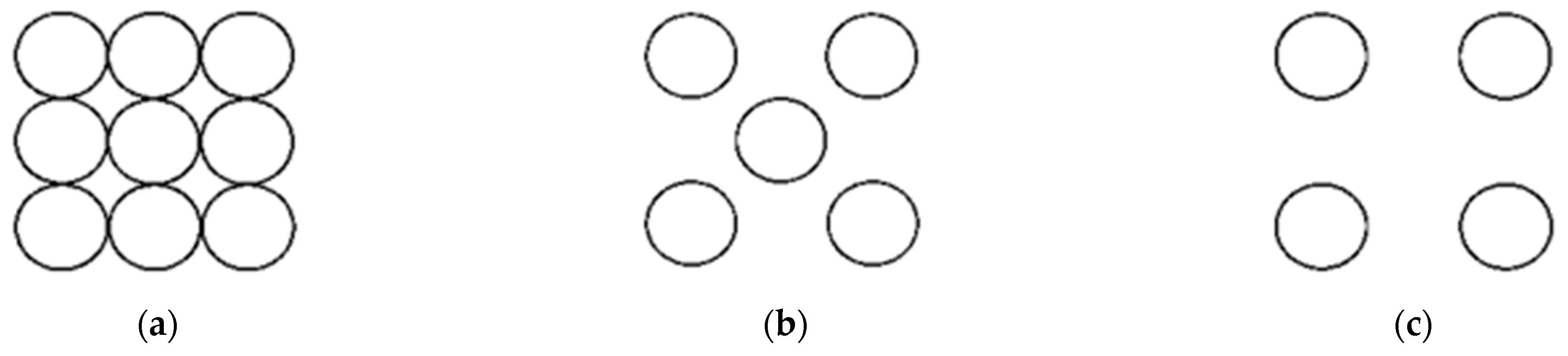
Figure 1. Roughness types. (a) Closely packed; (b) Medium packed; (c) Sparsely packed.
Wind 04 00018 g001
Figure 2. Imaginary part of the normalized effective impedance calculated using the Attenborough–Tolstoy impedance model for various roughness types.
Wind 04 00018 g002
Figure 3. Diagram of experimental setup.
Wind 04 00018 g003
Figure 4. Comparison of the measured excess attenuation to the analytical and parabolic equation theory using the Attenborough–Tolstoy effective impedance model. (a) Closely packed roughness; (b) Medium packed roughness; (c) Sparsely packed roughness. For all figures (ac), the sound source height, receiver height and horizontal distance between the two were 100 mm, 100 mm and 400 mm, respectively, for situation 1.
Wind 04 00018 g004aWind 04 00018 g004b
Figure 5. Comparison of the measured relative sound pressure level, Rel. SPL, to the analytical and parabolic equation theory using the Attenborough–Tolstoy effective impedance model for a closely packed roughness. The sound source height, receiver height and horizontal distance between the two were 200 mm, 20 mm, and 100 mm, respectively, for situation 2.
Wind 04 00018 g005
Figure 6. Simplified diagram of the scenario in mind for the parabolic equation method simulations.
Wind 04 00018 g006
Figure 7. Relative sound pressure level, Rel. SPL, against propagation range, measured at 2 m height. Calculated for various roughness types using the parabolic equation method.
Wind 04 00018 g007
Figure 8. Relative sound pressure level, Rel. SPL, map close to ground level. Calculated using the parabolic equation method. (a) Sparsely packed roughness; (b) Medium packed roughness; (c) Closely packed roughness.
Wind 04 00018 g008aWind 04 00018 g008b
Table 1. Roughness parameters.
Roughness TypeNumber per Unit Area, NCenter-Center Spacing, L (m)Coverage per Unit Area, n (%)
Closely packed13720.03378.5
Medium packed7000.04640
Sparsely packed3500.06520
Table 2. Roughness parameters for parabolic equation method.
Roughness TypeNumber per Unit Area, NCenter-Center Spacing, L (m)Coverage per Unit Area, n (%)
Closely packed60.48375.4
Medium packed30.68337.7
Sparsely packed11.36612.6
Table 3. Details of the predicted relative sound pressure level at 2 km over varying ground roughness types.
Roughness TypeRel. SPL at 2 km (dB)
Closely packed−4.9
Medium packed−3
Sparsely packed−0.6
Disclaimer/Publisher’s Note: The statements, opinions and data contained in all publications are solely those of the individual author(s) and contributor(s) and not of MDPI and/or the editor(s). MDPI and/or the editor(s) disclaim responsibility for any injury to people or property resulting from any ideas, methods, instructions or products referred to in the content.

