Novel Machine-Learning-Based Stall Delay Correction Model for Improving Blade Element Momentum Analysis in Wind Turbine Performance Prediction

Abstract

Wind turbine blades experience excessive load due to inaccuracies in the prediction of aerodynamic loads by conventional methods during design, leading to structural failure. The blade element momentum (BEM) method is possibly the oldest and best-known design tool for evaluating the aerodynamic performance of wind turbine blades due to its simplicity and short processing time. As the turbine rotates, the aerofoil lift coefficient enhances, notably in the rotor’s inboard section, relative to the value predicted by 2D experimentation or computational fluid dynamics (CFD) for the identical angle of attack; this is induced by centrifugal pumping action and the Coriolis force, thus delaying the occurrence of stall. This rotational effect is regarded as having a significant influence on the rotor blade’s aerodynamic performance, which the BEM method does not capture, as it depends on 2D aerofoil characteristics. Correction models derived from the traditional hard computing mathematical method are used in the BEM predictions to take into account stall delay. Unfortunately, it has been observed from the earlier literature that these models either utterly fail or inaccurately predict the enhancement in lift coefficient due to stall delay. Consequently, this paper proposes a novel stall delay correction model based on the soft computing technique known as symbolic regression for high-level precise aerodynamic performance prediction by the BEM process. In complement to the correction model for the lift coefficient, a preliminary correction model for the drag coefficient is also suggested. The model is engendered from the disparity in 3D and 2D aerofoil coefficients over the blade length for different wind speeds for the NREL Phase VI turbine. The proposed model’s accuracy is evaluated by validating the 3D aerofoil coefficients computed from the experimental results of a second wind turbine known as the MEXICO rotor.

1. Introduction

The rapid depletion of fossil fuels in recent decades has resulted in a scarcity of power generation. This intensifies the demand for alternate energy sources to fossil fuels. Wind energy has been acknowledged as one of the most intriguing renewable energy resources [1]. Wind turbine design is demanding in terms of both expense and time. Based on this, the engineering approach known as blade element momentum (BEM) was extensively employed in wind turbine blade design [2,3,4]. With the increasing dimensions of wind turbine blades, precise and efficient techniques for predicting aerodynamic loads and performance are anticipated [5]. The BEM method evaluates forces throughout the blade length and ultimately the torque and the engendered power by the rotor depending on wind speed, rotor design, and aerofoil characteristics ($C_L$ and $C_D$). Since wind turbine cross-sections are aerofoil-shaped, the BEM method requires aerofoil characteristics in order to evaluate sectional aerodynamic forces [4]. At low wind speeds, BEM predictions exhibit good accuracy, but at higher wind speeds, BEM fails due to massively separated flow conditions [4,6]. The characteristics of the aerofoil used in BEM are predicted from a 2D wind tunnel or CFD measurements [4,7]. Owing to the spanwise separated flow, there is an enhancement in the lift coefficient of the aerofoils of the rotating blade at the identical angle of attack compared to the 2D analysis of the aerofoil or 3D analysis of the aerofoil of a non-rotating blade, which delays stall. This phenomenon is called “stall delay” [3,4]. There is no conclusive knowledge regarding the causes of stall delay, however it is thought that when flow separation begins, a separated air mass on the suction face rotates with the blade due to centrifugal force. The separated air mass tends to approach the tip radially due to centrifugal force. This spanwise flow therefore enables Coriolis force to impact toward the trailing edge, resulting in a delay in stall initiation [4,5,6,8,9,10,11,12,13]. The second explanation in the literature [5,12,14] that contributes for the radial flow of the separated air mass is the dynamic pressure gradient along the length of the blade. Eventually, stall delay is a boundary layer impact that is speculated to be induced by centrifugal force, dynamic pressure gradient, or a blend of the two. Although technologically advanced wind turbines are pitch-controlled and therefore do not normally function in stall, stall in the inner section of the blade is inevitable once rated power is reached [15]. Failure to comprehend the effect of stall delay may lead to under-prediction of aerodynamic values and design failure. It is more effective at inboard portions and progressively drops towards the tip [4]. As a corollary, before utilising them in design, 2D aerofoil characteristics must be compensated for rotational impacts [4,5].

Himmelskamp [16] in the 1940s was the first to recognize the difference between lift coefficients for rotating and non-rotating aircraft propellers. Banks and Gadd [17] conducted a theoretical study and clarified how rotation delays separation and inferred that rotation induces the boundary layer to stabilize and resist separation. Stall delay was analysed and examined by Dwyer and McCroskey [18] on helicopter rotors. Later, in wind turbines, Milborrow [19] and Madsen and Christensen [20] noticed the stall delay effect. Variation in the predicted lift coefficient comparing rotating and non-rotating blades was shown by Ronsten [21] in his observational investigation. Figure 1 presents the estimated lift coefficient at 30 percent of the blade length from the work of Ronsten [21].

Wood [22], Narramore and Vermeland [23], and Snel et al. [24] conducted CFD evaluation in the early 1990s, with development of computers, to examine the consequences of stall delay. Numerous empirical correction models for wind turbine rotor design have been generated over the last few decades [4,11,15]. These were all three-dimensional correction models considering the impact of stall delay to correct 2D aerofoil characteristics. In 2001, NREL performed a blind test comparison relying on an interpretation of the experimental results from an NREL Phase VI turbine. Experts were urged to estimate the load values for the NREL Phase VI turbine without the actual experimental results being given to them [25]. Significant uncertainties were reported as compared with experimental results and estimated values.

Figure 1. $C_L$ vs. AoA for rotating blade (RB) and non–rotating blade (NRB) at 30 percent blade length [21].

Figure 1. $C_L$ vs. AoA for rotating blade (RB) and non–rotating blade (NRB) at 30 percent blade length [21].

Consequently, existing models to modify 2D aerofoil characteristics to depict stall delay effects were found to be incorrect. In 2002, Schreck and Robinson [14], using the results of the NREL Phase VI turbine experiment, utilised CFD to examine the influence of the radial pressure gradient on the stall delay mechanism. In 2008, in simulating the NREL Phase VI turbine, Breton et al. [11] utilised the lifting line-prescribed wake vortex theory to explore the performance of six correction models for stall delay (Snel, Chaviaropoulos and Hansen, Raj, Corrigan and Schilling, Bak, and Lindenburg models) and hypothesized that all these models end in over-prediction. Guntur et al. [15] conducted an equivalent test for the MEXICO rotor, and the selected correction models (Snel, Du and Selig, Chaviarpoulus and Hansen, Lindenburg, and Bak) failed to predict the 3D aerodynamic characteristics accurately. In prior work, the authors Kabir and Ng [4] compared 3D aerofoil coefficients computed throughout the blade length from NREL Phase VI turbine CFD simulation with values computed utilising BEM analysis employing four correction models (Snel, Lindenburg, Du and Selig, and Chaviarpoulus and Hansen models). It was found that these models over-predicted the lift coefficients and power computed, especially at high wind speeds. This was predominantly owing to the complexity of foreseeing the rotation effect on wind turbines, stressing the importance of developing an accurate numerical model. Guntur and Sørensen [15,26] used the Inverse BEM method to compute the angles of attack and the 3D aerofoil characteristics of the specific segments of turbine blades. Lately, Kabir and Ng [4] enhanced the Inverse BEM strategy as well as the computed angle of attack and 3D aerofoil characteristics of 18 Sections (5 sections regarded for experimental measurements and 13 additional sections as outlined in blade design) from full rotor CFD simulations of the NREL Phase VI turbine. Kabir and Ng [4] also proposed amendments to BEM analysis to account for the impact of local blade length using the angle of attack and aerofoil characteristics computed from Inverse BEM evaluation. Regrettably, the main purpose of using BEM analysis is pace and ease. Although the method of computing 3D aerofoil characteristics is precise, it is complex and requires substantial computational power to model CFD and perform Inverse BEM. Therefore, an optimal method must be established to reconcile precision and pace.

In this paper, a new empirical model derived from the soft computing technique called ‘Symbolic Regression’ is formulated for the correction of 2D aerofoil characteristics data to compensate for the stall delay in wind turbine blade design and performance analysis via BEM. This paper is structured as follows:

• A synopsis of the stall delay mechanism;
• A synopsis of the Blade Element Momentum theory and Inverse BEM theory;
• A brief description of existing correction models for stall delay used in BEM;
• Description of the NREL Phase VI turbine and MEXICO rotor experiments;
• Proposed new models;
• Results comparison to NREL Phase VI turbine and MEXICO rotor data, followed by discussion.

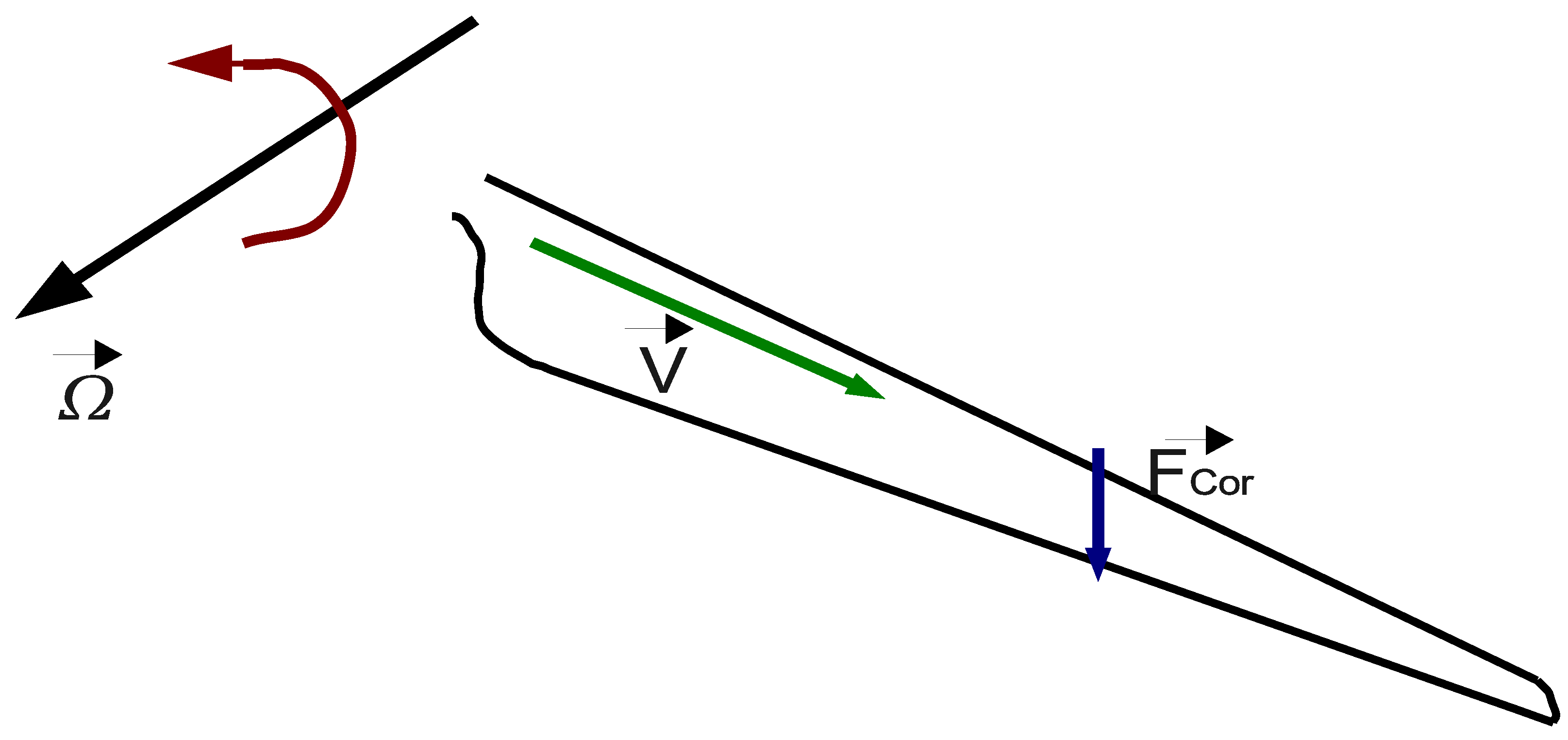
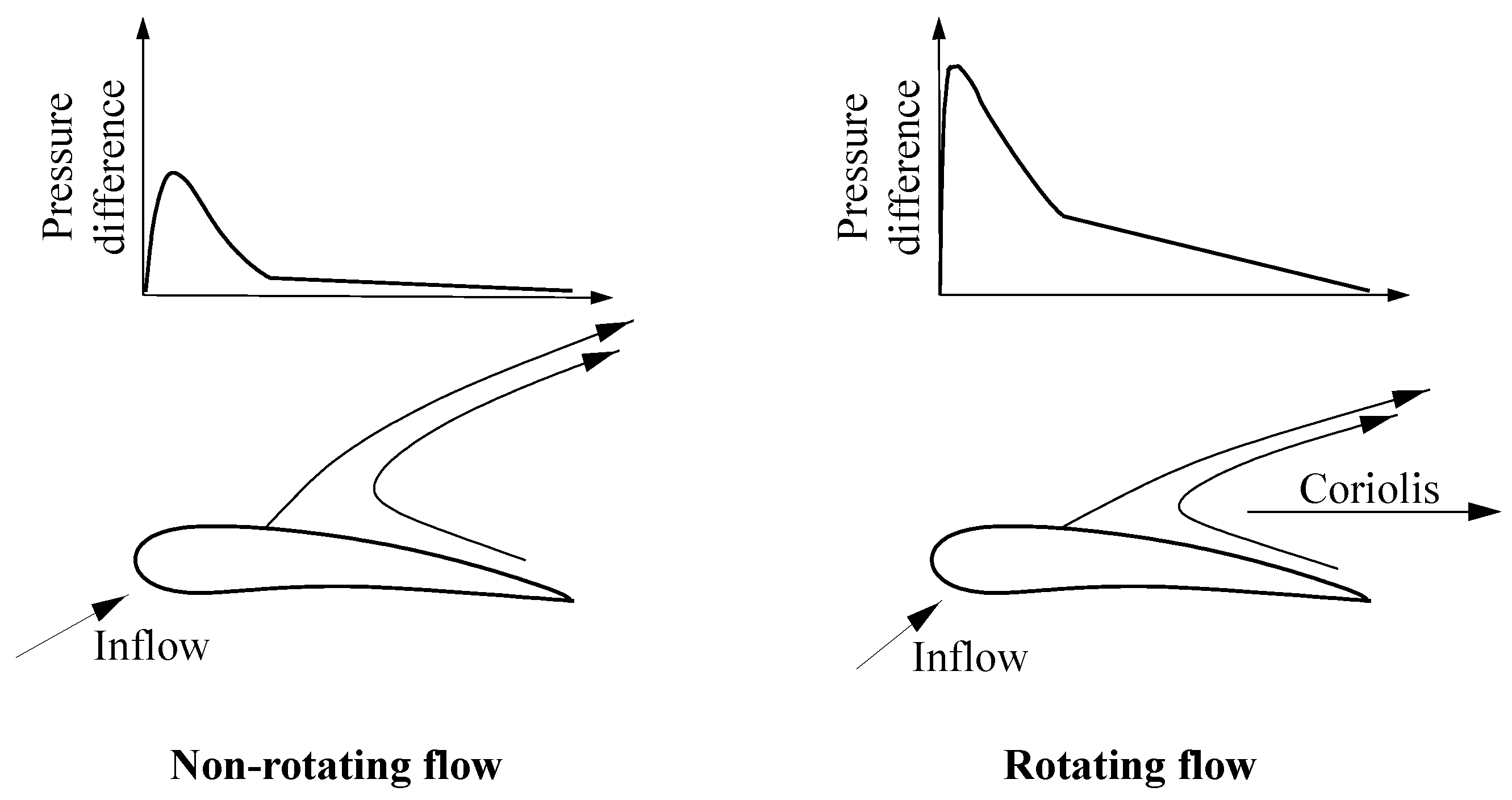
2. Stall Delay Mechanism

Stall delay is a boundary layer phenomenon that is primarily assumed to be attributable to centrifugal force, a dynamic pressure gradient, or a blend of both. Either or both of these responses stimulate spanwise flow, leading to formation of the Coriolis force [4,5,6,8,9,10,11,12,13,14,27,28,29], as shown in Figure 2. The Coriolis force acts from the leading edge to the trailing edge as a positive chord-wise pressure gradient, ensuing in stall delay, as shown in Figure 3. Figure 3 illustrates this phenomenon, where the pressure difference between the aerofoil’s suction side and pressure side is higher for a rotating flow than for a non-rotating flow due to the presence of Coriolis force, which increases the lift coefficient. At low wind speeds, which implies low angles of attack, the flow stays attached on the rotor’s suction side, and no stall emerges. Even though centrifugal force and the dynamic pressure gradient are present, their effects are modest since the flow passes over the blade in a brief period of time. When flow separation occurs at higher wind speeds (i.e., at higher angles of attack), a separated air mass persists along the suction surface and is subjected to centrifugal pumping and/or a dynamic pressure gradient. When spanwise flow occurs in a rotating reference frame, the Coriolis effect occurs, resulting in stall delay.

3. Blade Element Momentum Theory and Inverse BEM Theory

3.1. Blade Element Momentum Theory

Due to its simplicity and speed, the Blade Element Momentum (BEM) method is often utilised for wind turbine blade design and wind turbine performance analysis. The BEM methodology estimates forces throughout the blade length and ultimately the torque and the turbine power. Betz’s [30] and Glauert’s [31] research serve as the foundation for this concept. The BEM theory blends the concepts of momentum and blade element theories into one cohesive framework. The momentum balance on a rotating annular stream tube is described using the momentum theory, while the forces created by the aerofoil cross-section of the blade section are computed using the blade element theory. In BEM theory, a wind turbine blade is segmented into (N) elements. The intent is to establish a balance between the force imposed on the blade elements and the change of the momentum magnitude of the air between the upstream and downstream regions of the rotor based on these two theories in each element independently. In Burton et al. [8] and Hansen [32], the BEM method is properly delineated. The fundamental premise of BEM theory is that forces and velocities computed in each element are calculated independently and are unaffected by the adjacent elements. The aerofoil characteristics ($C_L$ and $C_D$) required by the blade element theory to calculate forces at each sectional element are generally obtained via wind tunnel or 2D CFD simulations. The three-dimensional (3D) and unsteady effects happening on the blade, such as yaw misalignment, wind shear, tower shadow, dynamic stall, dynamic inflow, and stall delay, cannot be captured directly by the BEM method [28,32,33,34]. The other effects are real-time, while the stall delay explained earlier raises the lift coefficient even under ideal conditions owing to blade rotation. Thus, it is necessary to first enhance BEM to take into account stall delay, followed by the inclusion of corrective models for additional real-time unsteady effects. In synopsis, traditional BEM theory is based on two-dimensional aerofoil characteristics that must be rectified for the rise in value caused by stall delay.

3.2. Inverse Blade Element Momentum Theory

The authors earlier [4] provided a comprehensive description of BEM analysis of the NREL Phase VI turbine using several aerofoil characteristic extrapolation techniques and different existing correction models for stall delay. The authors demonstrated that it is crucial to determine the optimal aerofoil characteristics ($C_{L,3D}$ and $C_{D,3D}$) throughout the blade length in order to improve the BEM model and narrow the disparity among 2D and 3D aerofoil characteristics. The computation of sectional AoA, $C_{L,3D}$, and $C_{D,3D}$ throughout the blade length has been accomplished using a variety of methodologies [26,35]. One of the strategies is the Inverse BEM method. This was a strategy utilised by the authors. In previous work [4], the authors validated their computation using other approaches used by other researchers to estimate the sectional $C_{L,3D}$ and $C_{D,3D}$ for the NREL Phase VI turbine. Inverse BEM analysis is carried out in the opposite way from BEM analysis, as the name indicates. In the conventional BEM analysis outlined above, at each element, based on the calculated AoA, $C_{L,2D}$, and $C_{D,2D}$, is supplied as key to determine the forces impacting that element. While in Inverse BEM analysis, the forces calculated from 3D CFD or experimental analysis were used to predict the aerofoil characteristics ($C_{L,3D}$ and $C_{D,3D}$) using the reverse approach to BEM [4].

4. Models for Stall Delay Correction in BEM Technique

The BEM process utilises the aerofoil sections’ $C_L$ and $C_D$ values throughout the blade length. Aerofoil characteristics are typically inferred from wind tunnels or 2D CFD tests. As stated in the preceding section, stall delay enhances $C_L$, notably on the inboard portions of the blade. There are numerous correction models to integrate BEM analyses to account for the impact of stall delay. The inaccuracies of various correction models for stall delay were outlined in Section 1. Breton et al. [11] compared the results of the NREL Phase VI turbine to six correction models for stall delay: Snel [36], Chaviaropoulos and Hansen [37], Raj [38], Corrigan and Schilling [39], Bak [40], and Lindenburg [9]. The models over-predicted the forces observed on a wind turbine blade throughout a variety of operating cases, while the model built by Lindenburg [9] was shown to perform the best across the set of scenarios investigated but still had substantial inadequacies. Guntur et al. [15] did an analogous test for the MEXICO rotor and compared it to five correction models: Snel [36], Du and Selig [41], Chaviarpoulus and Hansen [37], Lindenburg [9], and Bak [40]. None of the five correction models could accurately predict the 3D aerofoil characteristics [5,15]. Detailed assessments of the BEM analysis for the evaluation of the NREL Phase VI turbine were carried out in 2017 by Kabir and Ng [4]. They focused on the various extrapolation methods for the S809 aerofoil polar characteristics. They used an enhanced Inverse BEM strategy to predict $C_{L,3D}$ and $C_{D,3D}$ values from the full CFD rotor analysis throughout the blade length and compared their measured values with the corresponding BEM values, leveraging four different correction models for stall delay [4]: Snel [36], Du and Selig model [41], Chaviaropolous and Hansen [37], and Lindenburg [9]. It was observed that among the four models, the Lindenburg model was closest to the lift coefficients predicted by the Inverse BEM analysis of the 3D CFD simulation of the NREL Phase VI turbine.

Based on the disparity between 3D and 2D values and the use of symbolic regression as a soft computation methodology, a new correction model for stall delay is established in this work. Section 6 gives a brief synopsis of symbolic regression and the new model. It has previously been determined from three prior reports [4,11,15] that existing correction models for stall delay—Snel [36], Du and Selig [41], Chaviaropolous and Hansen [37], Raj [38], Corrigan and Schilling [39], and Bak [40]—are inaccurate; thus, these models are discarded for comparison in this study. Since the Lindenburg [9] model was determined to be the closest to the 3D lift coefficient among all models [4,11], it is used for comparison with our novel model. The general formulation for the correction models are given below:

$$C_{L,3D}=C_{L,2D}+f_L\left(2\pi \left(\alpha -{\alpha }_0\right)-C_{L,2D}\right)$$

(1)

$$C_{D,3D}=C_{D,2D}+f_D\left(C_{D,2D}-C_D(\alpha =0)\right)$$

(2)

where ${\alpha }_0$ is the AoA when the lift is zero, and $C_D(\alpha =0)$ is the drag coefficient when AoA is zero. In this article, we have also included two additional recent correction models for stall delay for comparison. The three models used for comparison in this present study are:

4.1. Lindenburg [9]

Lindenburg analysed the stall delay phenomenon thoroughly and inferred that centrifugal pumping was its primary cause. In addition, he developed a stall delay correction model based on centrifugal pumping. In his correction model, he extended the model developed by Snel et al. [24] by including the ratio of the rotational speed at the tip and the relative local velocity. However, he did not provide a correction model for drag.

$$f_L=3.1{\left(\frac{\Omega r}{U_{rel}}\right)}^2{\left(\frac{c}{r}\right)}^2$$

(3)

$$f_D=0$$

(4)

4.2. Dumitrescu and Cardos [42,43,44]

A semi-empirical model for rectifying the two-dimensional lift coefficient of aerofoils was built by Dumitrescu and Cardos. This model fails to rectify the drag coefficient correction.

$$f_L=\left[1-exp\left(-\frac{\gamma }{r/c-1}\right)\right],\gamma =1.25$$

(5)

$$f_D=0$$

4.3. Hamlaoui, Smaili and Fellouah Model [45]

This model was developed on the basis of an evaluation conducted between the two-dimensional lift coefficients and the NREL Phase VI turbine experimental results. This model also fails to rectify the drag coefficient correction.

$$f_L=a{e}^{-{\left(\frac{\alpha -b}{c}\right)}^2}$$

(6)

$$C_{L,3D}=C_{L,2D}+f_L\left(C_{L,2D}\right)$$

(7)

where a, b, and c are constants, and $\alpha$ is the effective angle of attack (radian). For spanwise positions below 0.30R, a is 1.45, b is 0.7, and, c is 0.2832. Constant a is 0.55, b is 0.3826, and c is 0.1188 for spanwise positions higher than 0.30R.

5. Description of Experiments of NREL Phase VI Turbine and MEXICO Rotor

5.1. NREL Phase VI Turbine Experiment

The NREL Phase VI turbine (10.06 m in diameter) is a two-bladed HAWT that has been rigorously evaluated in the NASA Ames 24.4 m × 36.6 m wind tunnel in a series of operating scenarios [46]. Throughout the span of the blade, the blades are tapered and twisted and incorporate an S809 aerofoil. A consistent rotational speed of nearly 72 revolutions per minute (rpm) was maintained regardless of the wind speed. The sectional pressure distributions were monitored using 22 pressure taps interspersed at five radial positions: 30 percent, 47 percent, 63 percent, 80 percent, and 95 percent of the span. The sectional normal and tangential forces were evaluated by summing the surface pressures at all 22 of these points at each radial position. The technical report [46] has more specific details of the experiment. The experimental data from Sequence S with an axial inflow condition was/is utilised in the authors’ prior and current research. In a previous study [4], unsteady RANS (URANS) CFD simulations were conducted by the authors for inflow wind speeds of 7 m/s, 10 m/s, 15 m/s, 20 m/s, and 25 m/s employing the advanced sliding mesh method. $C_{L,3D}$ and $C_{D,3D}$ were calculated by employing Inverse BEM analysis at 18 radial positions (supplementary to the five radial positions used for experimental investigations, thirteen other positions were examined).

5.2. MEXICO Experiment

The Mexnext Phase III project was a global partnership led by the Netherlands’ Energy Research Centre (ECN) [47]. In 2018, the findings of the NEW MEXICO experiment, which was conducted in the German–Dutch wind tunnel, DNW, with an open section measuring 9.5 m × 9.5 m, became accessible [47]. The MEXICO rotor blade is 4.5 m in diameter and is composed of three aerofoils: DU91-W2-250, RISØ-A2-21, and NACA 64-418, from 20 to 45.6 percent of blade length, 54.4 to 65.6 percent of blade length, and 74.4 to 100 percent of blade length, respectively. The entire blade is twisted and tapered, with a global pitch angle of −2.3${}^{\circ }$. Experiments were conducted in the wind tunnel at 10 m/s, 15 m/s, and 24 m/s with the blade rotating at 425.1 rpm. Axial inflow was taken into account in this analysis, and the influence of blade yaw was not considered. The pressure was measured using pressure sensors positioned at five distinct blade sections: 25 percent, 35 percent, 60 percent, 82 percent, and 92 percent of the blade length. The authors in their previous work [48] used the sliding mesh approach to perform both Unsteady RANS (URANS) and LES CFD analysis for inlet wind speeds of 10 m/s, 15 m/s, and 24 m/s.

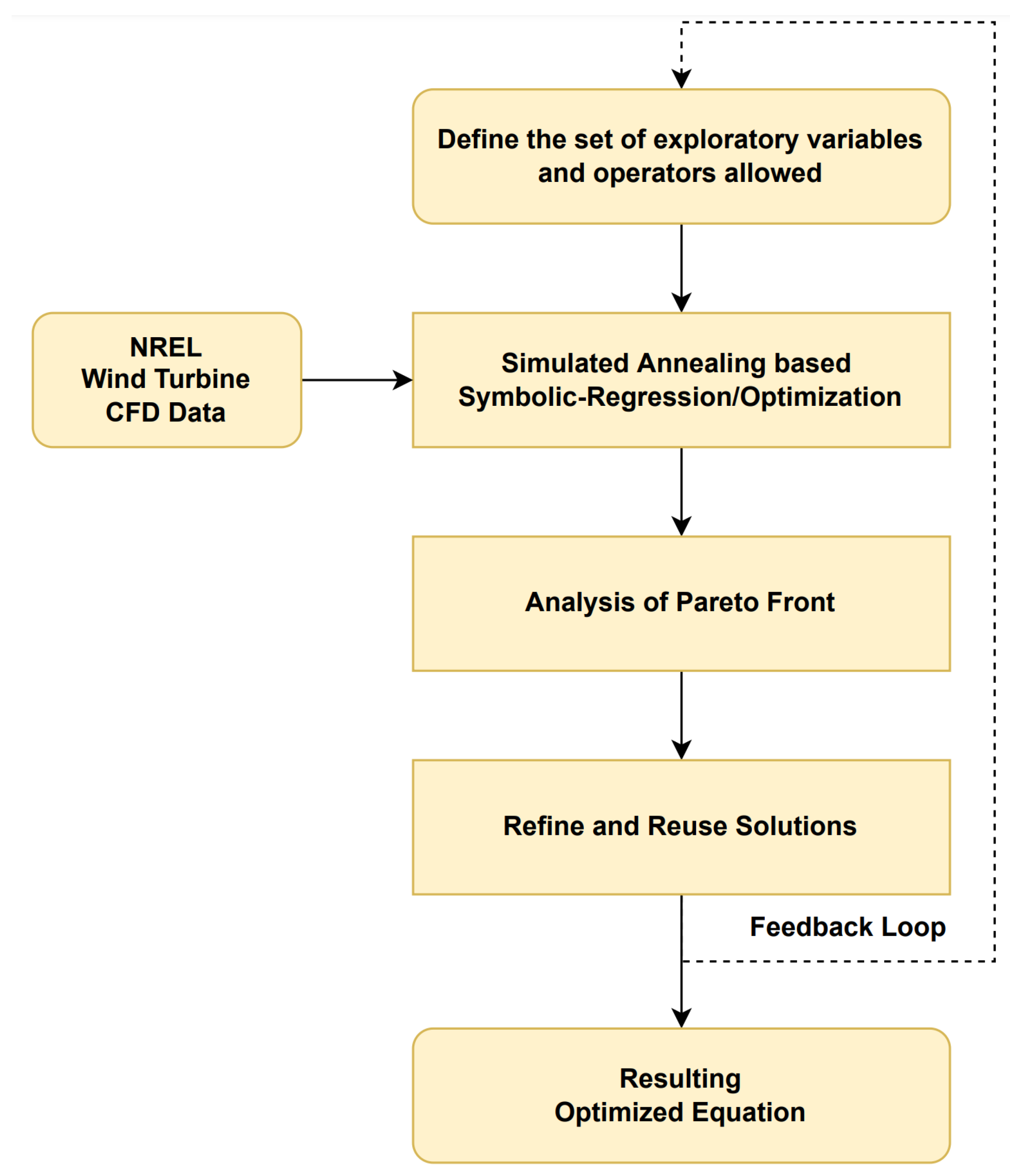
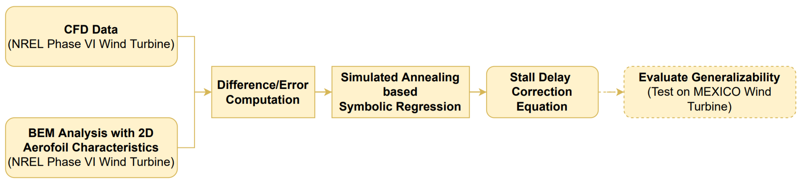
6. Symbolic Regression

Artificial intelligence (AI) is gaining popularity in several fields, from basic domestic appliances such as washing machines to advanced automated medical diagnosis [49,50,51,52]. The behaviour of AI is close to that of the human brain and can draw conclusions primarily based on constrained and particular facts from earlier studies [53]. Soft computing is a subset of artificial intelligence that deals with methods for conducting predicted qualitative and logical cognition [53,54]. Zadeh [55] coined the word “soft computing” to describe an alternate to traditional (hard) computing. Hard computation is a traditional problem-solving strategy that involves specifically defined computational or mathematical models, which requires a long period of computing and is inefficient in many complex real-world scenarios [54,56,57]. Evolutionary computation, fuzzy logic, probabilistic reasoning, neural networks, expert systems, data mining, and machine learning are some of the most important soft computational methods or techniques [54,57,58]. In this research, a soft computing technique known as regression analysis is utilised. Regression analysis is a statistical modelling technique used to determine a mathematical relationship between dependent (target) and independent (explanatory) variables [59,60]. In regression techniques such as polynomial regression, a model structure is first hypothesized, and then the coefficients are fit to the training data; however, symbolic regression is a distinct type of regression technique that involve both the discovery of the model structure and the coefficients within that model structure [61].

Symbolic regression is a widely used technique for the approximation of mathematical functions [62]. It explores the mathematical space to find the most desirable metamodel by a structured manner of modifying operators in a set of explicit formulae. Various formulae explored in symbolic regression can be expressed utilising a tree structure. A combinatoric optimization technique is used to obtain the best tree structure. The notable benefit of symbolic regression is its interpretability and capability to capture the underlying physics from data [63]. Symbolic regression has several advantages compared to other regression techniques, such as flexibility in the choice of operators, class of functions, and expression size. Symbolic regression to determine mathematical functions can be performed using several techniques such as genetic programming (GP) [64] and simulated annealing (SA) [65]. Although genetic programming- and simulated annealing-based symbolic regression utilize a tree structure to search for the optimal mathematical expression, the algorithmic searching methods are fundamentally different. A genetic algorithm starts with a population of possible solutions, and at each step (generation), it chooses pairs of a possible solution, joins them (crossover), and applies random changes (mutation). In contrast, simulated annealing takes a population and applies a metaheuristic function to approximate the global optimum in the large search space; this reduces the population’s random variation (rate, quantity, and type). The primary advantage of simulated annealing over genetic programming is its capability to arrive at a global minimum, and other advantages include the ease of determining constants and lower relative computational cost [63]. The overall procedure utilised in this work is illustrated in Figure 4.

Simulated annealing-based symbolic regression’s general idea is to have an overall look at all the components of the solution space at the start of the search, and to track one solution in the space of possible solutions. The parameters are adjusted gradually during each iteration, and the algorithm decides to either continue with the current solution or select the neighbouring solution based on probabilities (which decay over time). If the algorithm continuously accepts large adjustments during the optimization process, the starting parameters can be adjusted by reannealing. In symbolic regression, complex functions tend to fit the data better; however, complex functions are prone to over-fitting and are difficult to interpret. Therefore the objective is to determine a mathematical expression that is both simple (minimize the complexity) and fits the data (maximize the metamodel quality) using a MultiObjective Combinatorial Optimization (MOCO) method such as Pareto simulated annealing. A detailed algorithm for implementation of Pareto simulated annealing-based symbolic regression can be found in [63], and it was performed here using TuringBot python library on an AMD Ryzen™ 9 5900 CPU with 24 threads for about 1200 CPU hours. The authors described the limitations of machine learning-based models with training and test data derived from the findings of a single wind turbine simulation in one of their earlier publications [66]. It is advised to have data from various wind turbines in order to achieve generalizability. Since the experimental results of the NREL Phase VI wind turbine and MEXICO rotor are well acknowledged and often utilised, training data from the NREL Phase VI wind turbine and test data from the MEXICO rotor are utilised in this work.

6.1. Dataset

The training data were obtained from the unsteady RANS (URANS) CFD simulations of the NREL Phase VI wind turbine employing the advanced sliding mesh method from the authors’ prior work [4]. Aerofoil characteristics $C_{L,3D}$ and $C_{D,3D}$ were calculated by employing Inverse BEM analysis at 18 radial positions for different inlet wind speeds of 7 m/s, 10 m/s, 15 m/s, 20 m/s, and 25 m/s.

For validation, a hold-out cross-validation strategy was considered in this study to avoid overfitting: 20 percent of the training data was held-out to perform hyper-parameter optimization. The hyper-parameters that were optimized include the coefficients of the obtained functional form.

The testing data to ensure the generalizability of the proposed model were from experimental data of the MEXICO rotor [47,48]. The test data included the sectional aerofoil characteristics at five distinct radial positions (25 percent, 35 percent, 60 percent, 82 percent, and 92 percent) obtained at inlet wind speeds of 10 m/s, 15 m/s, and 24 m/s.

6.2. Model Evaluation

The model obtained from symbolic regression should fit well with the training and validation data. For this, we calculate the Root Mean Squared Error (RMSE):

$$RMSE=\sqrt{\frac{{\sum }_{i=1}^N{\left(\mathrm{Actual}{Y}_i-\mathrm{Predicted}f\left(x_i\right)\right)}^2}{N}}$$

(8)

If a change in model structure or model coefficients improves the obtained model (RMSE decreases), the change is accepted [63]; using this iterative process, a final model that is compact, interpretable, and fits the training and validation data well is obtained. Other details of the training process, such as defining exploratory variables and solution search options, can be found in Section 7.

7. New Empirical Model for Stall Delay

A total of six non-dimensional exploratory variables, including the tip-speed ratio defined as ($\lambda =\Omega R/U_{\infty }$), the ratio of local to total radius of the wind turbine ($r/R$), the ratio of local chord to local radius of the wind turbine ($c/r$), the ratio of inflow wind to relative velocity ($U_{\infty }/U_{rel}$), ${\lambda }_r$ defined as (${\lambda }_r=\Omega r/U_{\infty }$), and ${\lambda }_{rel}$ defined as (${\lambda }_{rel}=\Omega r/U_{rel}$), were formulated, and their values were extracted from NREL wind turbine data (see Section 5.1). The objective of the Pareto simulated annealing-based symbolic regression algorithm is to determine a mathematical expression to model the target variable $f_L$ (stall delay correction parameter for lift) and $f_D$ (stall delay correction parameter for drag) based on Equations (9) and (10), respectively.

$$f_L=f(\lambda ,\frac{r}{R},\frac{c}{r},\frac{U_{\infty }}{U_{rel}},{\lambda }_r,{\lambda }_{rel})$$

(9)

$$f_D=g(\lambda ,\frac{r}{R},\frac{c}{r},\frac{U_{\infty }}{U_{rel}},{\lambda }_r,{\lambda }_{rel})$$

(10)

After determining the expressions for stall delay correction parameters $f_L$ and $f_D$, the three-dimensional aerodynamic coefficients ($C_{L,3D}$ and $C_{D,3D}$) can be computed from two-dimensional aerodynamic coefficients ($C_{L,2D}$ and $C_{D,2D}$) utilising Equations (1) and (2), respectively.

The six non-dimensional exploratory variables that were included to model the target stall delay correction parameters $f_L$ and $f_D$ are shown in Equations (9) and (10), respectively. Parameter selection (feature selection) to model the target variable using exploratory variables is performed by the algorithm automatically. This step ensures that the model is constructed only using parameters (features) that capture the underlying physics. Mathematical operators (×, ÷, exponent, and square root) were chosen for the expression search, and remaining operators such as +, −, and trigonometric values were excluded in order to obtain a generalised expression that is not limited to a specific range of the input parameters and to ensure that the resulting expression is not very sensitive to small changes to the input.

$$f_L=C_1\times e^{\left(\frac{C_2}{\lambda \times \frac{c}{r}}\right)}$$

(11)

$$f_D=C_3\times \lambda \times e^{\frac{c/r}{{(C_4\times \lambda )}^{\lambda }}}$$

(12)

The proposed stall delay correction model determined using Pareto simulated annealing-based symbolic regression is given in Equations (11) and (12), where $C_1=1.425330$, $C_2=1.261960$, $C_3=0.267109$, $C_4=0.337107$. The choice of exploratory parameters is crucial for the symbolic regression model’s capability to capture the underlying physics; therefore, the non-dimensional exploratory parameters (see Equations (11) and (12)) considered in this study were chosen based on extensive literature review. Further, the variables $\lambda$ (tip speed ratio) and $c/r$ (ratio of local chord to local radius) were selected automatically based on their capability to capture the underlying physics. The compact size of the expression and choice of operators in the expression reaffirms that the model is not overfit to the data. In addition, the obtained model is also validated on MEXICO rotor experimental results. The overall workflow of this study is shown in Figure 5.

8. Results and Discussions

This section portrays the comparative study focused on the Blade Element Momentum evaluation of the NREL Phase VI turbine and MEXICO rotor. In prior strategies for deriving corrective models, data from only one rotor were typically employed. The Lindenburg model, for instance, is based on NREL Phase VI turbine experiments. The correction computed for certain cases may not be appropriate in the other cases of different wind turbines. As a basis, the model in this study was developed using data from NREL Phase VI turbine analysis and verified using MEXICO rotor analysis. The authors Kabir and Ng [4] executed earlier CFD assessments of the NREL Phase VI turbine and computed $C_{L,3D}$ and $C_{D,3D}$ values using an enhanced Inverse BEM method because the aerofoil coefficients from experiments were not directly available. Kabir and Ng [4] verified their forecasts with other previous works [67,68,69,70,71] at five radial positions (30 percent, 47 percent, 63 percent, 80 percent, and 95 percent). Therefore, if the prediction at five radial positions is accurate, the values predicted at other radial positions (13 positions used for the design) would be accurate as well. In contrast to earlier models, which only use data from the five radial positions specified in the experimental details, additional radial positions were utilised for data creation in order to obtain a more accurate corrective model. In this comparison, 2D aerofoil characteristics of an S809 aerofoil from Delft University of Technology (DUT) wind tunnel analysis for Reynolds numbers of $1\times {10}^6$ up to ${20.6}^{\circ }$ AoA were used, and the Viterna and Corrigon method [72] for polar extrapolation was used, as described by Kabir and Ng [4]. Since the MEXICO rotor was deployed for validation, the sectional aerofoil characteristics at five distinct radial positions (25 percent, 35 percent, 60 percent, 82 percent, and 92 percent) were calculated from the experimental results using the Inverse BEM method executed in MATLAB. In this comparative investigation, BEM results without and with correction models for stall delay are compared to 3D aerofoil coefficients of the NREL Phase VI turbine, followed by validation with MEXICO rotor results.

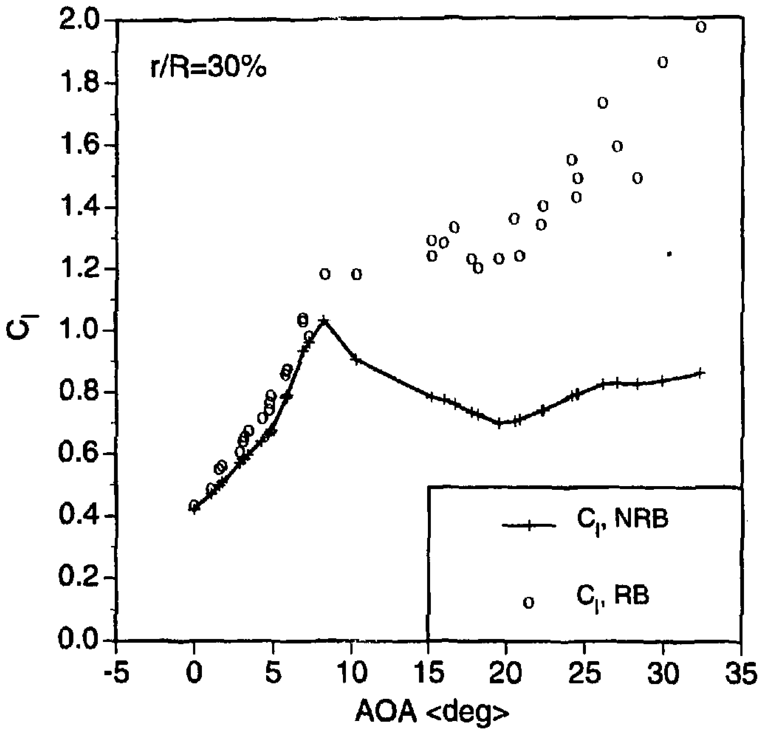
8.1. 3D Aerodynamic Characteristics

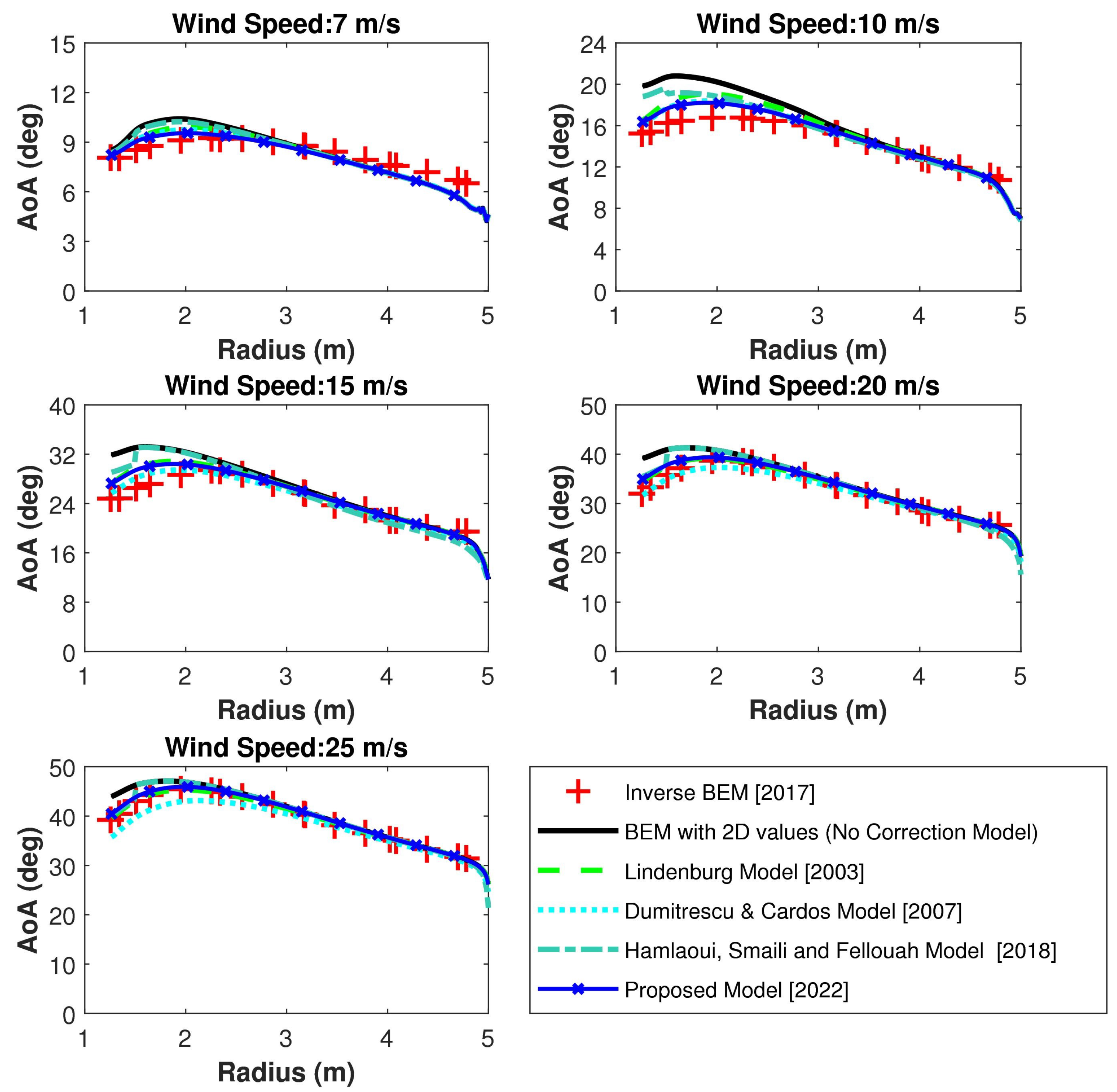
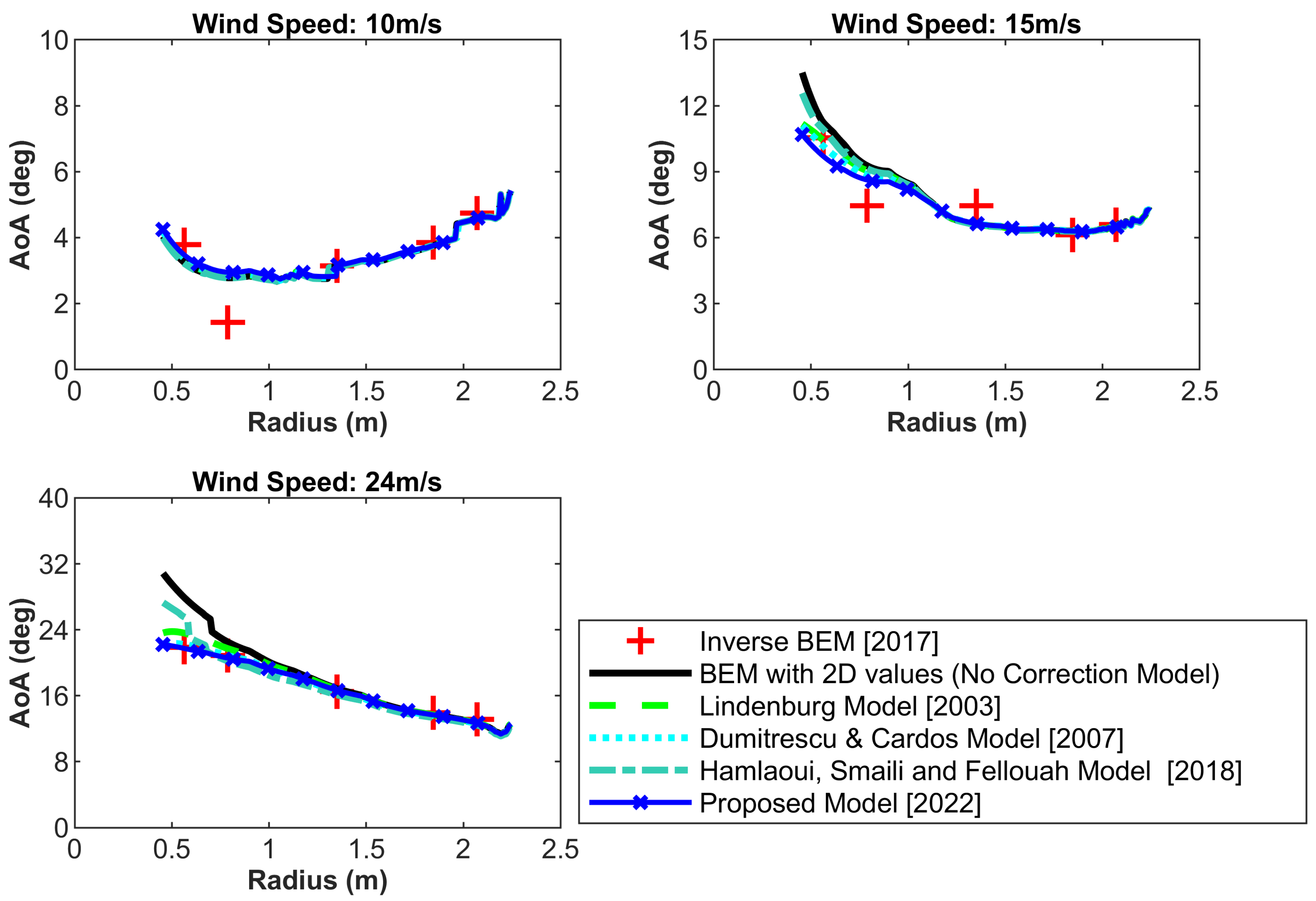
8.1.1. Angle of Attack Distribution

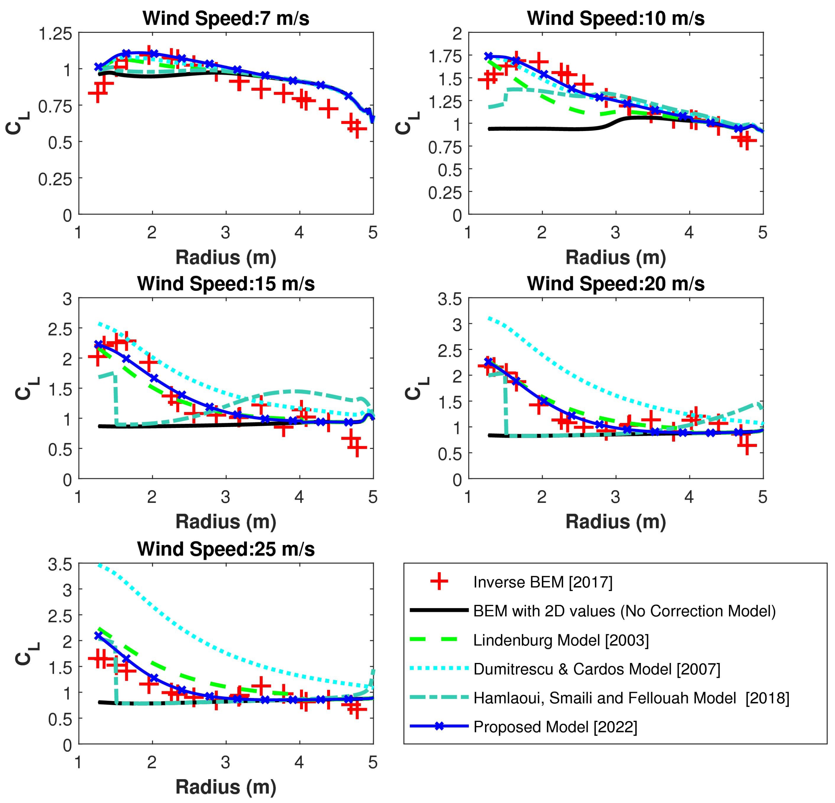
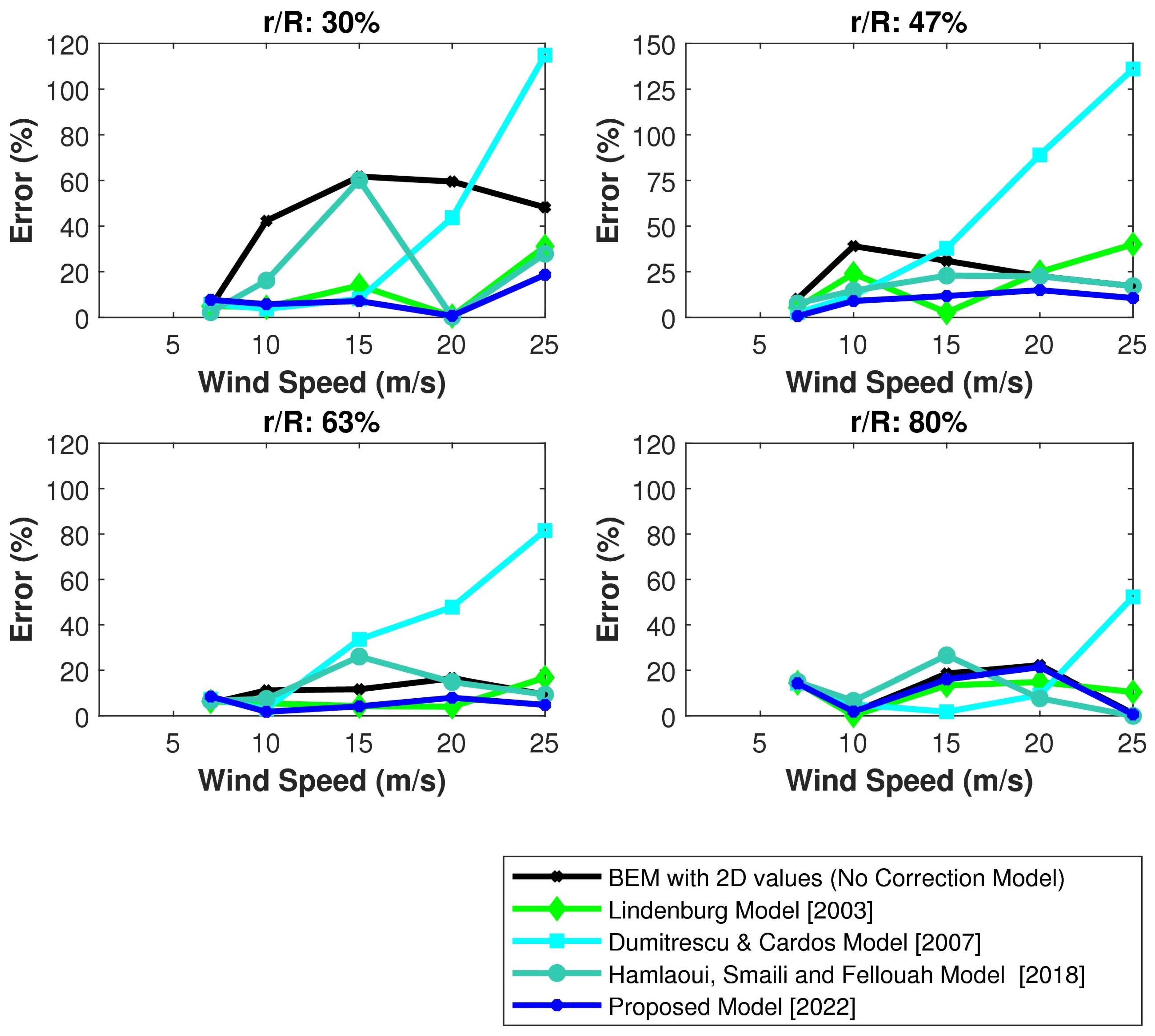
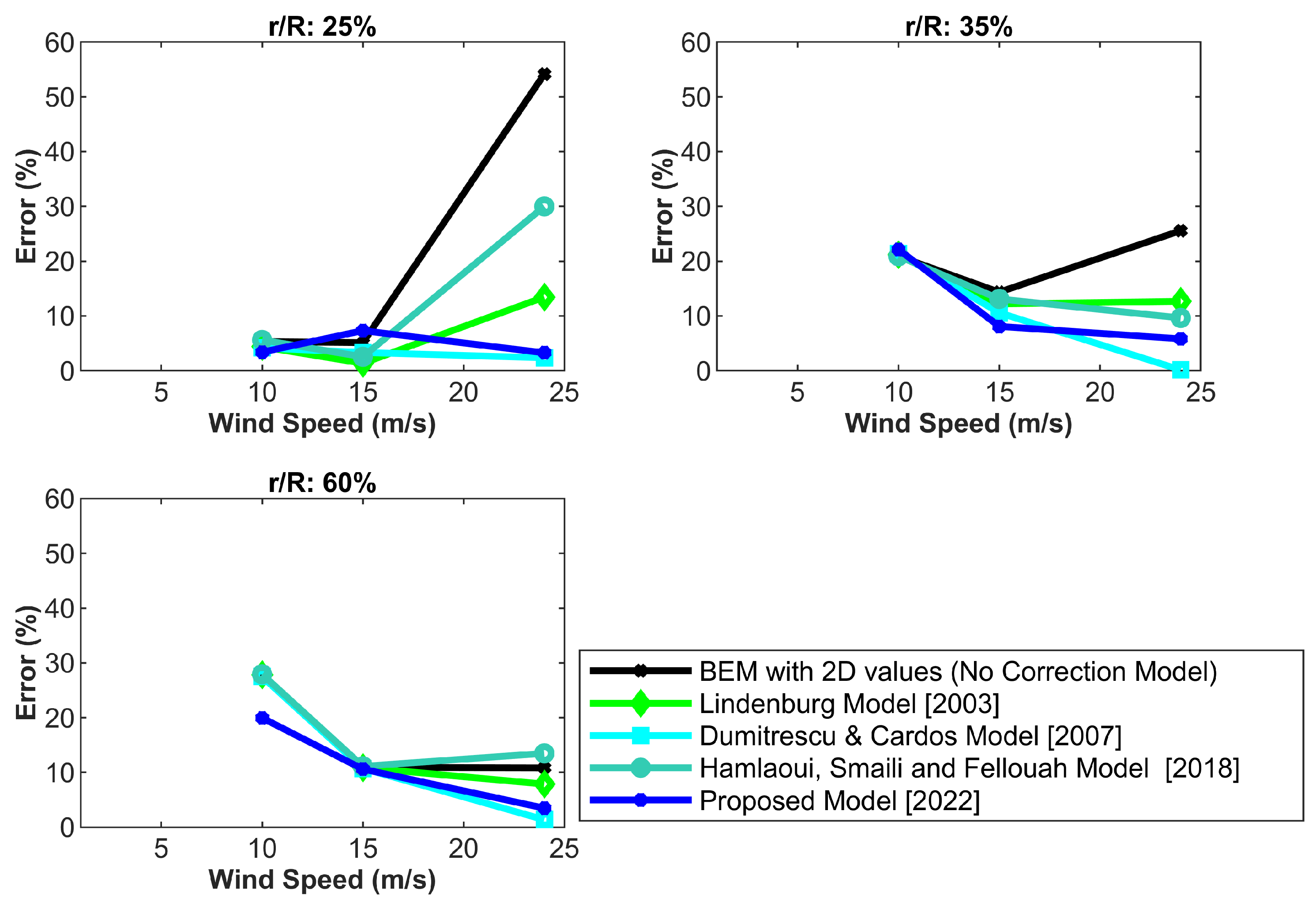
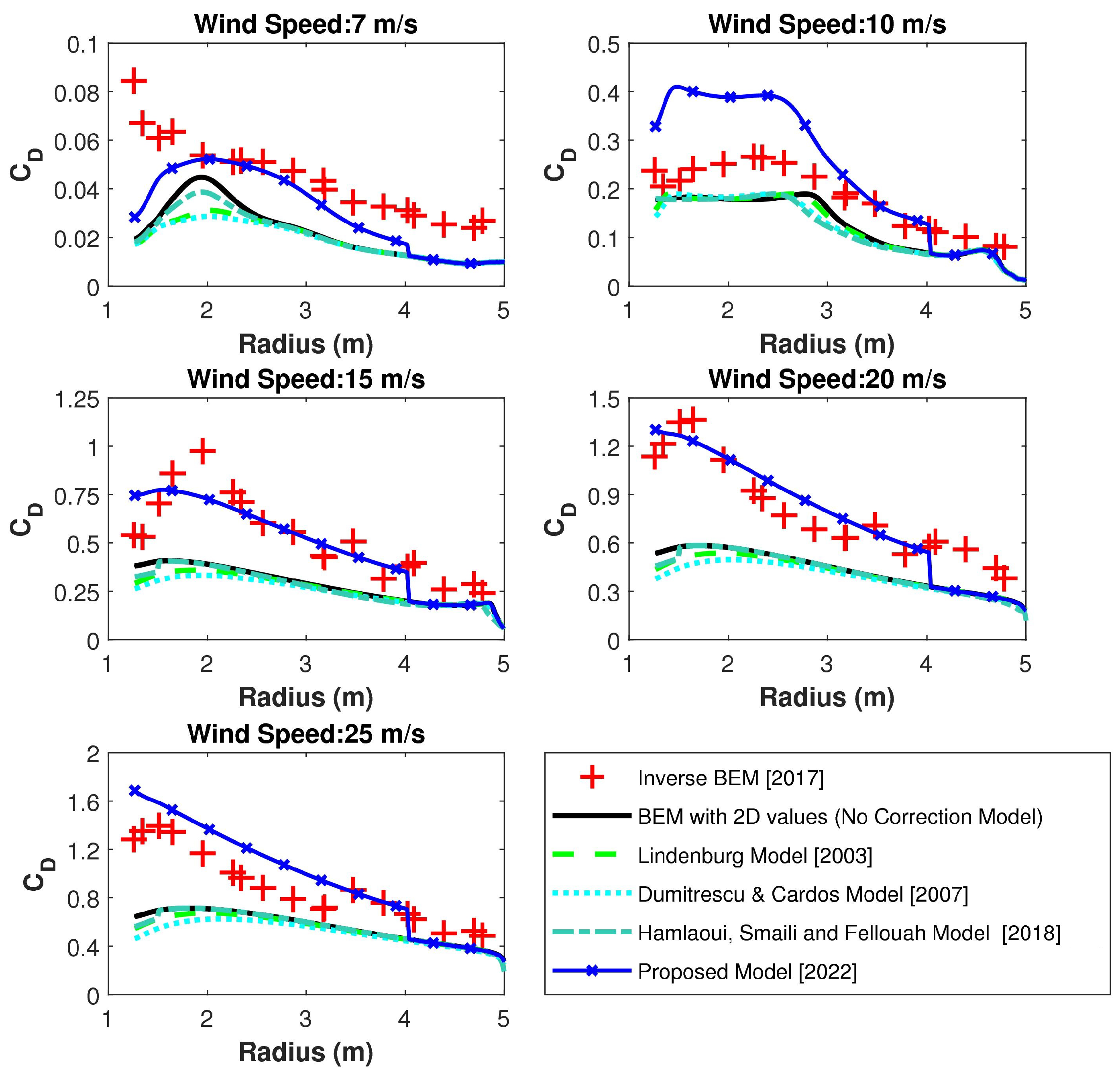
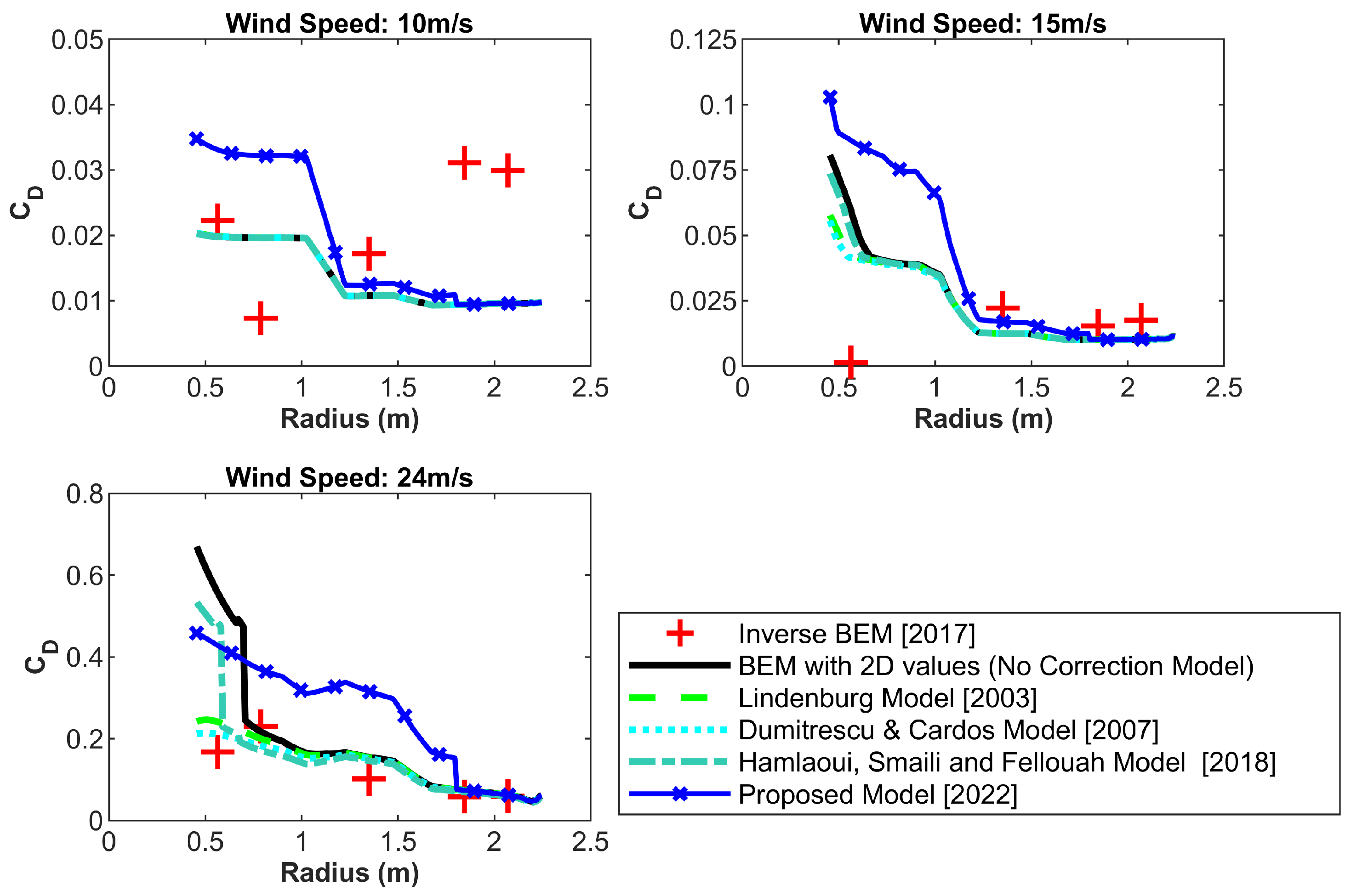
Figure 6 depicts the distribution of angles of attack over the blade length for wind speeds ranging from 7 to 25 m/s, as calculated from the BEM assessment of the NREL Phase VI turbine without and with distinct correction models for stall delay. Figure 7 presents a comparison of the distribution of angles of attack over the blade length for the MEXICO rotor at wind speeds of 10 m/s, 15 m/s, and 24 m/s. It is essential to realise that whereas correction models for stall delay alter anticipated forces on the blades, the influence on distribution of angles of attack is minimal. The sole exception is when the correction models for stall delay predict very high load variations in the area of the root. In these cases, a comparable local variation in angles of attack is created at the root, as predicted by BEM analysis with correction models for stall delay, which are close to 3D values predicted by Inverse BEM analyses, but BEM with no correction models overestimates angles of attack.

8.1.2. Comparison of $C_L$ Prediction throughout the Blade Length

Figure 8 illustrates the contrast of the estimated $C_L$ value throughout the blade length by the BEM assessment without and with the different existing correction models for stall delay and the model proposed with the $C_{L,3D}$ value obtained from the CFD analyses of the NREL Phase VI turbine for wind speeds of 7 m/s, 10 m/s, 15 m/s, 20 m/s, and 25 m/s. BEM predicts the enhancement in lift coefficient attributable to stall delay quite decently up to a wind speed of 10 m/s with all correction models for stall delay [4]. With increasing wind speed, BEM with previous correction models for stall delay, such as the Dumitrescu and Cardos model [42,43,44], estimate higher $C_L$ values in comparison to $C_{L,3D}$ calculation from the CFD study for the NREL Phase VI turbine [4]. The Lindenburg model [9] substantially overpredicts at extremely high wind speed of 25 m/s, as predicted earlier by Breton et al. [11] and Kabir and Ng [4]; however, for other wind speeds, the trajectory of increase in $C_L$ throughout the blade length is close to the $C_{L,3D}$ throughout the blade length. The Hamlaoui, Smaili and Fellouah model [45] for r/R < 30 percent, which is considered to be the lower inboard region of the blade, and for r/R > 50 percent, which is considered to be the top half of the blade, gives predictions comparable to the 3D values. However, the value of $C_L$ shows a profound downward trend for r/R between 30 percent and 50 percent, ignoring the effect of stall delay. The root cause of this tendency is that Hamlaoui et al. [45] employed values from only five radial positions: 30 percent, 47 percent, 63 percent, 80 percent, and 95 percent. It is worth noting that just around 30 percent of the r/R is located in the inboard portion, where the effect of stall delay is strongest, whereas the other four radial positions are almost on the blade’s upper half. As a consequence, they incorporated two components in their correction models: r/R < 30 percent and r/R > 30 percent. However, because the second component is based on values predicted above 47 percent, this model fails to estimate the effect of stall delay between 30 and 47 percent. As a corollary, 3D values computed at additional radial positions (0.250R, 0.267R, 0.328R, 0.390R, 0.450R, 0.510R, 0.570R, 0.633R, 0.691R, and 0.750R) were also included in estimating the correction models in our work. Therefore, for all wind speeds, the current proposed model determines results close to the $C_{L,3D}$ for the NREL Phase VI turbine. The accuracy of the proposed model is confirmed by computing the error percentage at four radial positions (0.30R, 0.47R, 0.63R, and 0.80R) considered in the experimental analysis and is presented in Figure 9. As recognised, the percentage of error calculated from the proposed method is predominantly less compared to the other models. The proposed model can only be used up to 0.8R, whereas the calculated values of $C_L$ at r/R > 80 percent are $C_{L,2D}$ values without any added correction. Unlike the inboard section, $C_{L,3D}$ in the tip region is lower than $C_{L,2D}$. This is due to tip vortices with the secondary flow generated at the tip [5,11]. The current model is only meant to take into account stall delay; therefore, the correction model is only proposed up to 0.8 R. For this reason, radial positions smaller than 0.8 R are represented in the error comparison for both the NREL Phase VI and MEXICO rotors. In the future, a new model will be proposed to account for the correction in the reduction of the lift coefficient due to the effect of tip vortices. Figure 10 depicts the $C_L$ distribution estimated from BEM analysis without and with correction models for stall delay along the MEXICO rotor’s blade length for three distinct wind speeds. Figure 11 shows the error comparison for $C_L$ prediction at three distinct radial positions (0.25R, 0.35R, and 0.60R) utilised in the experimental analysis, ignoring radial positions above 0.8R. Almost all models forecast closure values with the experimental data at wind speeds of 10 m/s and 15 m/s; however, at 24 m/s, the Dumitrescu and Cardos [42,43,44] model and the proposed model are quite similar to 3D values obtained from the experimental data, while the Lindenburg model [9] is slightly lower but follows the same trend. The Hamlaoui, Smaili and Fellouah model [45], on the other hand, is a total catastrophe. As per Figure 10 and Figure 11, the proposed model outperforms the existing correction models for stall delay.

8.1.3. Comparison of $C_D$ Prediction throughout the Blade Length

Figure 12 compares the estimated $C_D$ value throughout the blade length using BEM without or with the correction models for stall delay using the $C_{D,3D}$ values obtained through the Inverse BEM method of CFD analysis at wind speeds of 7 m/s, 10 m/s, 15 m/s, 20 m/s, and 25 m/s for the NREL Phase VI turbine. The BEM utilising earlier correction models for stall delay predicts lower $C_D$ values than the $C_{D,3D}$ determined from CFD analysis using the Inverse BEM approach. The values estimated based on earlier correction models for stall delay considered for comparison in this study are close to the $C_{D,2D}$ values since these models do not account for drag coefficient corrections. On the contrary, since there was a divergence noticed in $C_{D,3D}$ and $C_{D,2D}$ for all wind speeds, a new model is proposed and compared in Figure 12. While previous models did not even approach the 3D values, the proposed model predicts extremely close at high wind speeds (15 m/s, 20 m/s, and 25 m/s) and relatively close at low wind speeds (7 m/s and 10 m/s). Figure 12 compares the estimated $C_D$ value throughout the blade length using BEM without or with the correction models for stall delay with $C_{D,3D}$ values obtained through the Inverse BEM method of CFD analysis on wind speeds of 10 m/s, 15 m/s, and 24 m/s for the MEXICO rotor. Figure 12 and Figure 13 show that for the NREL Phase VI turbine, $C_{D,3D}$ is often higher than $C_{D,2D}$, indicating that rotational effects were associated with a notable drag rise, but for the MEXICO rotor, rotational effects were associated with a small drag drop. Ivan Harreaz [5] exploited OpenFOAM to do CFD simulations of the MEXICO rotor and calculated sectional $C_{L,3D}$ and $C_{D,3D}$ at three distinct wind speeds. Ivan Harreaz [5] also noticed a similar discrepancy in $C_D$ predictions. Other drag correction models, such as those by Chaviaropolous and Hansen [37] and Raj [38], anticipate an increase in $C_D$, but the Corrigan and Schillings [39] and Du and Selig [41,73] models predict a decrease in $C_D$. Other models, such as those by Snel [36], Lindenburg [9], Dumitrescu and Cardos [42,43,44], and Hamlaoui , Smaili and Fellouah [45], have not proposed models or taken into account a $C_D$ discrepancy. In fact, it can be noticed from Figure 13 that there is no discernible difference between the $C_{D,3D}$ and $C_{D,2D}$ values for the MEXICO rotor. Furthermore, according to Ivan Harreaz [5], rotational effects have minimal influence on $C_D$ (except at r/R = 60 percent). Guntur et al. [15], who used the MEXICO rotor to evaluate correction models, came to the conclusion that $C_D$ correction may not be essential. Ivan Harreaz [5] concluded that the effect of rotation on drag appears to be aerofoil-type dependant, which we concur with. Since, as stated in Section 1 of this paper, the main concern of this work is to predict lift enhancement due to stall delay. Further, the effect of rotation on drag is minimal compared to its effect on lift, and because this work employs a novel dimension of using Machine Learning (ML), we propose a preliminary model for drag correction depending on the predictions of the NREL Phase VI turbine. Despite the fact that this model is dependent on NREL Phase VI turbine data, the forecast for the MEXICO rotor is still close. In the future, an additional relevant parameter representing aerofoil type will be taken into account, and a new model for drag correction with greater accuracy will be built that enables forecasting of both increases and decreases in the drag coefficient based on aerofoil type.

9. Conclusions and Future Works

Practically, direct CFD analyses of wind farms with a significant number of wind turbines are not feasible. Hence in CFD analyses of wind farms, indirect rotor modelling, such as Actuator Disk (AD), Actuator Line (AL), and Actuator Surface (AS) modelling, are necessary. This indirect rotor modelling depends on BEM analyses for aerodynamic phenomena performance. Hence, if the prediction of BEM is wrong, that leads to incorrect CFD analyses. Therefore, accurate prediction from BEM is essential for the CFD analyses of a wind farm. This work, thus, takes account of an attempt to improve the precision of BEM in the prediction of aerodynamic loads. In this investigation, a new correction model was derived using soft computing called Symbolic Regression based on the disparity between 3D CFD observations and 2D values of aerofoil coefficients throughout the blade length for different wind speeds of the NREL Phase VI turbine. It has been noted from the literature that correction models for stall delay derived from conventional hard computing techniques are not accurate enough. Contrarily, BEM predicts the lift and drag coefficient closure of the CFD results while using the new correction model for stall delay for the NREL Phase VI turbine [4]. The proposed model is validated using 3D aerofoil characteristics collected from the MEXICO rotor experimental results with an Inverse BEM approach. The proposed model effectively predicts closure for lift coefficient comparisons, but the drag coefficients are slightly over-predicted. This might be due to the effect of rotation on drag, which differs based on aerofoil type. The drag coefficient increases with rotation for the NREL Phase VI turbine but decreases for the MEXICO rotor. This research focuses on the rise in lift coefficients caused by stall delay at the inboard sections; therefore, significant emphasis is placed on lift coefficient correction models. A preliminary model for the drag coefficient is also suggested and found to be adequate. The proposed model for lift correction is good for r/R < 80 percent because at r/R > 80 percent, 3D lift coefficients are lower than 2D lift coefficients due to the influence of tip vortices; we are now developing a new model to compute the decrease in lift coefficients at the blade’s tip. In addition, we are focusing on a novel correction model for drag coefficients based on the type of aerofoil.

Ongoing research seeks to improve rotor and wake aerodynamic prediction in wind farm modelling and optimization. The authors focused on wake aerodynamics in their earlier works [1,74,75] and derived empiric relationships specifically to determine the wake velocity and turbulence intensity. In this article, the authors emphasised one of the unsteady effects in rotor aerodynamics modelling called stall delay to accurately model three-dimensional rotational augmentation effect. In the future, ML-based models will be developed for other unsteady 3D effects such as dynamic stall [76,77,78], dynamic inflow [79], yaw misalignment [80], wind shear [81], and tower shadow [76] to improve rotor modelling techniques. Subsequently, both these rotor and wake aerodynamic modelling strategies can be utilised to extract data to optimize axial flow wind farms to estimate the power from a given landscape.

References

1. Kabir, I.F.S.A.; Safiyullah, F.; Ng, E.Y.K.; Tam, V.W. New analytical wake models based on artificial intelligence and rivalling the benchmark full-rotor CFD predictions under both uniform and ABL inflows. Energy 2020, 193, 116761. [Google Scholar] [CrossRef]
2. Liu, S.; Janajreh, I. Development and application of an improved blade element momentum method model on horizontal axis wind turbines. Int. J. Energy Environ. Eng. 2012, 3, 30. [Google Scholar] [CrossRef] [Green Version]
3. Sun, Z.; Chen, J.; Shen, W.Z.; Zhu, W.J. Improved blade element momentum theory for wind turbine aerodynamic computations. Renew. Energy 2016, 96, 824–831. [Google Scholar] [CrossRef]
4. Kabir, I.F.S.A.; Ng, E.Y.K. Insight into stall delay and computation of 3D sectional aerofoil characteristics of NREL phase VI wind turbine using inverse BEM and improvement in BEM analysis accounting for stall delay effect. Energy 2017, 120, 518–536. [Google Scholar] [CrossRef]
5. Herráez, I.; Stoevesandt, B.; Peinke, J. Insight into rotational effects on a wind turbine blade using Navier–Stokes computations. Energies 2014, 7, 6798–6822. [Google Scholar] [CrossRef] [Green Version]
6. Plaza, B.; Bardera, R.; Visiedo, S. Comparison of BEM and CFD results for MEXICO rotor aerodynamics. J. Wind Eng. Ind. Aerodyn. 2015, 145, 115–122. [Google Scholar] [CrossRef]
7. Manwell, J.F.; McGowan, J.G.; Rogers, A.L. Wind Energy Explained: Theory, Design and Application; John Wiley & Sons: Hoboken, NJ, USA, 2010. [Google Scholar]
8. Burton, T.; Jenkins, N.; Sharpe, D.; Bossanyi, E. Wind Energy Handbook; John Wiley & Sons: Hoboken, NJ, USA, 2011. [Google Scholar]
9. Lindenburg, C. Investigation into Rotor Blade Aerodynamics; ECN-C–03-025; Energy Research Centre of the Netherlands (ECN) Wind Energy Publication: Petten, The Netherlands, 2003. [Google Scholar]
10. Hu, D.; Hua, O.; Du, Z. A study on stall-delay for horizontal axis wind turbine. Renew. Energy 2006, 31, 821–836. [Google Scholar] [CrossRef]
11. Breton, S.P.; Coton, F.N.; Moe, G. A study on rotational effects and different stall delay models using a prescribed wake vortex scheme and NREL phase VI experiment data. Wind Energy Int. J. Prog. Appl. Wind Power Convers. Technol. 2008, 11, 459–482. [Google Scholar] [CrossRef]
12. Breton, S.P. Study of the Stall Delay Phenomenon and of Wind Turbine Blade Dynamics Using Numerical Approaches and NREL’s Wind Tunnel Tests. 2008. Available online: https://ntnuopen.ntnu.no/ntnu-xmlui/bitstream/handle/11250/231375/124628_FULLTEXT02.pdf?sequence=1 (accessed on 20 September 2022).
13. Elgammi, M.; Sant, T. A new stall delay algorithm for predicting the aerodynamics loads on wind turbine blades for axial and yawed conditions. Wind Energy 2017, 20, 1645–1663. [Google Scholar] [CrossRef]
14. Schreck, S.; Robinson, M. Rotational augmentation of horizontal axis wind turbine blade aerodynamic response. Wind Energy Int. J. Prog. Appl. Wind Power Convers. Technol. 2002, 5, 133–150. [Google Scholar] [CrossRef]
15. Guntur, S.; Bak, C.; Sørensen, N.N. Analysis of 3D stall models for wind turbine blades using data from the MEXICO experiment. In Proceedings of the 13th International Conference on Wind Engineering, Amsterdam, The Netherlands, 10–15 July 2011. [Google Scholar]
16. Himmelskamp, H. Profile Investigations on a Rotating Airscrew; Ministry of Aircraft Production: Göttingen, Germany, 1947. [Google Scholar]
17. Banks, W.; Gadd, G. Delaying effect of rotation on laminar separation. AIAA J. 1963, 1, 941. [Google Scholar] [CrossRef]
18. Dwyer, H.; McCROSKE, W. Crossflow and unsteady boundary-layer effects on rotating blades. AIAA J. 1971, 9, 1498–1505. [Google Scholar] [CrossRef]
19. Milborrow, D. Changes in aerofoil characteristics due to radial flow on rotating blades. In Proceedings of the 7th BWEA Conference, Oxford, UK, 27–29 March 1985. [Google Scholar]
20. Madsen, H.A.; Christensen, H. On the relative importance of rotational, unsteady and three-dimensional effects on the HAWT rotor aerodynamics. Wind. Eng. 1990, 14, 405–415. [Google Scholar]
21. Ronsten, G. Static pressure measurements on a rotating and a non-rotating 2.375 m wind turbine blade. Comparison with 2D calculations. J. Wind Eng. Ind. Aerodyn. 1992, 39, 105–118. [Google Scholar] [CrossRef]
22. Wood, D. A three-dimensional analysis of stall-delay on a horizontal-axis wind turbine. J. Wind Eng. Ind. Aerodyn. 1991, 37, 1–14. [Google Scholar] [CrossRef]
23. Narramore, J.; Vermeland, R. Navier-Stokes calculations of inboard stall delay due to rotation. J. Aircr. 1992, 29, 73–78. [Google Scholar] [CrossRef]
24. Snel, H.; Houwink, R.; Bosschers, J. Sectional Prediction of Lift Coefficients on Rotating Wind Turbine Blades in Stall. 1994. Available online: https://www.osti.gov/etdeweb/biblio/6693027 (accessed on 20 September 2022).
25. Simms, D.; Schreck, S.; Hand, M.; Fingersh, L.J. NREL Unsteady Aerodynamics Experiment in the NASA-Ames Wind Tunnel: A Comparison of Predictions to Measurements; Technical Report; National Renewable Energy Lab.: Golden, CO, USA, 2001. [Google Scholar]
26. Guntur, S.; Sørensen, N.N. An evaluation of several methods of determining the local angle of attack on wind turbine blades. J. Phys. Conf. Ser. 2014, 555, 012045. [Google Scholar] [CrossRef] [Green Version]
27. Pereira, R. Validating the Beddoes-Leishman Dynamic Stall Model in the Horizontal Axis Wind Turbine Environment. Master’s Thesis, Department of Control and Operations, Delft University of Technology, Delft, The Netherlands, 2010. [Google Scholar]
28. Kabir, I.F.S.A. Improvement of Bem Analysis to Incorporate Stall Delay Effect and the Study of Atmospheric Boundary Layer Effect on the Wake Characteristics of NREL Phase VI Turbine. Ph.D. Thesis, School of Mechanical and Aerospace Engineering, Nanyang Technological University, Singapore, 2018. [Google Scholar]
29. Lindenburg, C. Modelling of rotational augmentation based on engineering considerations and measurements. In Proceedings of the European Wind Energy Conference, London, UK, 22–25 November 2004; pp. 22–25. [Google Scholar]
30. Betz, A. Das Maximum der theoretisch möglichen Ausnutzung des Windes durch Windmotoren. Z. Fur Das Gesamte Turbinenwesten 1920, 26, 307–309. [Google Scholar]
31. Glauert, H. The Elements of Aerofoil and Airscrew Theory; Cambridge University Press: Cambridge, UK, 1983. [Google Scholar]
32. Hansen, M. Aerodynamics of Wind Turbines, 2nd ed.; Earthscan: London, UK, 2008. [Google Scholar]
33. Hansen, A.; Butterfield, C. Aerodynamics of horizontal-axis wind turbines. Annu. Rev. Fluid Mech. 1993, 25, 115–149. [Google Scholar] [CrossRef]
34. Leishman, J.G. Challenges in modelling the unsteady aerodynamics of wind turbines. Wind Energy Int. J. Prog. Appl. Wind Power Convers. Technol. 2002, 5, 85–132. [Google Scholar] [CrossRef]
35. Rahimi, H.; Schepers, J.; Shen, W.Z.; García, N.R.; Schneider, M.; Micallef, D.; Ferreira, C.S.; Jost, E.; Klein, L.; Herráez, I. Evaluation of different methods for determining the angle of attack on wind turbine blades with CFD results under axial inflow conditions. Renew. Energy 2018, 125, 866–876. [Google Scholar] [CrossRef] [Green Version]
36. Snel, H.; Houwink, R.; Bosschers, J.; Piers, W.; Van Bussel, G.J.; Bruining, A. Sectional Prediction of sD Effects for Stalled Flow on Rotating Blades and Comparison with Measurements. 1993. Available online: https://www.osti.gov/etdeweb/biblio/6222685 (accessed on 20 September 2022).
37. Chaviaropoulos, P.; Hansen, M.O. Investigating three-dimensional and rotational effects on wind turbine blades by means of a quasi-3D Navier-Stokes solver. J. Fluids Eng. 2000, 122, 330–336. [Google Scholar] [CrossRef]
38. Raj, N.V. An Improved Semi-Empirical Model for 3-D Post-Stall Effects in Horizontal Axis Wind Turbines. Ph.D. Thesis, University of Illinois at Urbana-Champaign, Urbana-Champaign, IL, USA, 2000. [Google Scholar]
39. Corrigan, J.J.; Schillings, J. Empirical model for stall delay due to rotation. In Proceedings of the American Helicopter Society Aeromechanics Specialists Conference, San Francisco, CA, USA, 19–21 January 1994; pp. 1–16. [Google Scholar]
40. Bak, C.; Johansen, J.; Andersen, P.B. Three-dimensional corrections of airfoil characteristics based on pressure distributions. In Proceedings of the European Wind Energy Conference, Athens, Greece, 7 February–2 March 2006; pp. 1–10. [Google Scholar]
41. Du, Z.; Selig, M. A 3-D stall-delay model for horizontal axis wind turbine performance prediction. In Proceedings of the 1998 ASME Wind Energy Symposium, Reno, NV, USA, 12–15 January 1998; p. 21. [Google Scholar]
42. Dumitrescu, H.; Cardoş, V.; Dumitrache, A. Modelling of inboard stall delay due to rotation. J. Physics Conf. Ser. 2007, 75, 012022. [Google Scholar] [CrossRef] [Green Version]
43. Dumitrescu, H.; Cardoş, V. Inboard boundary layer state on wind turbine blades. ZAMM-J. Appl. Math. Mech. Für Angew. Math. Und Mech. Appl. Math. Mech. 2009, 89, 163–173. [Google Scholar] [CrossRef]
44. Dumitrescu, H.; Cardos, V. Inboard stall delay due to rotation. J. Aircr. 2012, 49, 101–107. [Google Scholar] [CrossRef] [Green Version]
45. Hamlaoui, M.N.; Smaili, A.; Fellouah, H. Improved BEM Method for HAWT Performance Predictions. In Proceedings of the 2018 International Conference on Wind Energy and Applications in Algeria (ICWEAA), Algiers, Algeria, 6–7 November 2018; pp. 1–6. [Google Scholar]
46. Hand, M.; Simms, D.; Fingersh, L.; Jager, D.; Cotrell, J.; Schreck, S.; Larwood, S. Unsteady Aerodynamics Experiment Phase VI: Wind Tunnel Test Configurations and Available Data Campaigns; Technical Report; National Renewable Energy Lab.: Golden, CO, USA, 2001. [Google Scholar]
47. Schepers, J.; Lutz, T.; Boorsma, K.; Gomez-Iradi, S.; Herraez, I.; Oggiano, L.; Rahimi, H.; Schaffarczyk, P.; Pirrung, G.; Madsen, H.A.; et al. Final Report of Iea Wind Task 29 Mexnext (Phase 3); ECN: Petten, The Netherlands, 2018. [Google Scholar]
48. Purohit, S.; Kabir, I.F.S.A.; Ng, E.Y.K. On the Accuracy of uRANS and LES-Based CFD Modeling Approaches for Rotor and Wake Aerodynamics of the (New) MEXICO Wind Turbine Rotor Phase-III. Energies 2021, 14, 5198. [Google Scholar] [CrossRef]
49. Khan, M.Z.; Gajendran, M.K.; Lee, Y.; Khan, M.A. Deep Neural Architectures for Medical Image Semantic Segmentation. IEEE Access 2021, 9, 83002–83024. [Google Scholar] [CrossRef]
50. Gajendran, M.K.; Khan, M.Z.; Khattak, M.A.K. ECG Classification using Deep Transfer Learning. In Proceedings of the 2021 4th International Conference on Information and Computer Technologies (ICICT), Kahului, Maui Island, HI, USA, 11–14 March 2021; pp. 1–5. [Google Scholar]
51. Jahmunah, V.; Ng, E.; San, T.R.; Acharya, U.R. Automated detection of coronary artery disease, myocardial infarction and congestive heart failure using GaborCNN model with ECG signals. Comput. Biol. Med. 2021, 134, 104457. [Google Scholar] [CrossRef]
52. Gajendran, M.K.; Rohowetz, L.J.; Koulen, P.; Mehdizadeh, A. Novel machine-learning based framework using electroretinography data for the detection of early-stage glaucoma. Front. Neurosci. 2022, 15, 869137. [Google Scholar] [CrossRef]
53. Karray, F.; Karray, F.O.; De Silva, C.W. Soft Computing and Intelligent Systems Design: Theory, Tools, and Applications; Pearson Education: London, UK, 2004. [Google Scholar]
54. Londhe, S.N.; Dixit, P.R. Genetic programming: A novel computing approach in modeling water flows. In Genetic Programming-New Approaches and Successful Applications; IntechOpen Publishing: London, UK, 2012. [Google Scholar]
55. Yager, R.R.; Zadeh, L.A.; Kosko, B.; Grossberg, S. Fuzzy Sets, Neural Networks, and Soft Computing; Technical Report; John Wiley & Sons, Inc.: Hoboken, NJ, USA, 1994. [Google Scholar]
56. Magdalena, L. What is soft computing? Revisiting possible answers. Int. J. Comput. Intell. Syst. 2010, 3, 148–159. [Google Scholar]
57. Ibrahim, D. An overview of soft computing. Procedia Comput. Sci. 2016, 102, 34–38. [Google Scholar] [CrossRef] [Green Version]
58. Safiyullah, F.; Sulaiman, S.; Naz, M.; Jasmani, M.; Ghazali, S. Prediction on performance degradation and maintenance of centrifugal gas compressors using genetic programming. Energy 2018, 158, 485–494. [Google Scholar] [CrossRef]
59. Draper, N.R.; Smith, H. Applied Regression Analysis; John Wiley & Sons: Hoboken, NJ, USA, 1998; Volume 326. [Google Scholar]
60. Chatterjee, S.; Hadi, A.S. Regression Analysis by Example; John Wiley & Sons: Hoboken, NJ, USA, 2015. [Google Scholar]
61. Smits, G.F.; Kotanchek, M. Pareto-front exploitation in symbolic regression. In Genetic Programming Theory and Practice II; Springer: Berlin/Heidelberg, Germany, 2005; pp. 283–299. [Google Scholar]
62. Morales, C.O.; Vázquez, K.R. Symbolic regression problems by genetic programming with multi-branches. In Proceedings of the Mexican International Conference on Artificial Intelligence, Mexico City, Mexico, 26–30 April 2004; pp. 717–726. [Google Scholar]
63. Stinstra, E.; Rennen, G.; Teeuwen, G. Metamodeling by symbolic regression and Pareto simulated annealing. Struct. Multidiscip. Optim. 2008, 35, 315–326. [Google Scholar] [CrossRef]
64. Schmidt, M.; Lipson, H. Distilling free-form natural laws from experimental data. Science 2009, 324, 81–85. [Google Scholar] [CrossRef] [PubMed]
65. Kirkpatrick, S.; Gelatt, C.D.; Vecchi, M.P. Optimization by simulated annealing. Science 1983, 220, 671–680. [Google Scholar] [CrossRef]
66. Gajendran, M.K.; Kabir, I.F.S.A.; Purohit, S.; Ng, E. On the Limitations of Machine Learning (ML) Methodologies in Predicting the Wake Characteristics of Wind Turbines. In Renewable Energy Systems in Smart Grid; Springer: Berlin/Heidelberg, Germany, 2022; pp. 15–23. [Google Scholar]
67. Sørensen, N.N.; Michelsen, J.; Schreck, S. Navier–Stokes predictions of the NREL phase VI rotor in the NASA Ames 80 ft × 120 ft wind tunnel. Wind Energy Int. J. Prog. Appl. Wind Power Convers. Technol. 2002, 5, 151–169. [Google Scholar] [CrossRef]
68. Johansen, J.; Sørensen, N.N. Aerofoil characteristics from 3D CFD rotor computations. Wind Energy Int. J. Prog. Appl. Wind Power Convers. Technol. 2004, 7, 283–294. [Google Scholar] [CrossRef]
69. Tangler, J.; Kocurek, D. Wind turbine post-stall airfoil performance characteristics guidelines for blade-element momentum methods. In Proceedings of the 43rd AIAA Aerospace Sciences Meeting and Exhibit, Reno, NV, USA, 10–13 January 2005; p. 591. [Google Scholar]
70. Sant, T.; van Kuik, G.; Van Bussel, G. Estimating the angle of attack from blade pressure measurements on the NREL phase VI rotor using a free wake vortex model: Axial conditions. Wind Energy Int. J. Prog. Appl. Wind Power Convers. Technol. 2006, 9, 549–577. [Google Scholar] [CrossRef]
71. Schepers, J.; Van Rooij, R. Analysis of Aerodynamic Measurements on a Model Wind Turbine Placed in the NASA-Ames Tunnel. Contribution of ECN and TUD to IEA Wind Task XX. 2008. Available online: https://publications.tno.nl/publication/34628905/hf75V2/e08052.pdf (accessed on 20 September 2022).
72. Viterna, L.A.; Corrigan, R.D. Fixed pitch rotor performance of large horizontal axis wind turbines. In Proceedings of the NASA Lewis Research Center: Energy Production and Conversion Workshop, Cleveland, OH, USA, 1 January 1982; Volume 1. [Google Scholar]
73. Du, Z.; Selig, M. The effect of rotation on the boundary layer of a wind turbine blade. Renew. Energy 2000, 20, 167–181. [Google Scholar] [CrossRef]
74. Kabir, I.F.S.A.; Ng, E.Y.K. Effect of different atmospheric boundary layers on the wake characteristics of NREL phase VI wind turbine. Renew. Energy 2019, 130, 1185–1197. [Google Scholar] [CrossRef]
75. Purohit, S.; Kabir, I.F.S.A.; Ng, E.Y.K. Evaluation of three potential machine learning algorithms for predicting the velocity and turbulence intensity of a wind turbine wake. Renew. Energy 2022, 184, 405–420. [Google Scholar] [CrossRef]
76. Moriarty, P.J.; Hansen, A.C. AeroDyn Theory Manual; Technical report; National Renewable Energy Lab.: Golden, CO, USA, 2005. [Google Scholar]
77. Bangga, G.; Lutz, T.; Arnold, M. An improved second-order dynamic stall model for wind turbine airfoils. Wind Energy Sci. 2020, 5, 1037–1058. [Google Scholar] [CrossRef]
78. Küppers, J.P.; Reinicke, T. A WaveNet-Based Fully Stochastic Dynamic Stall Model. In Wind Energy Science Discussions; Copernicus GmbH: Göttingen, Germany, 2022; pp. 1–24. Available online: https://wes.copernicus.org/preprints/wes-2022-13/ (accessed on 20 September 2022).
79. Ferreira, C.; Yu, W.; Sala, A.; Viré, A. Dynamic inflow model for a floating horizontal axis wind turbine in surge motion. Wind Energy Sci. 2022, 7, 469–485. [Google Scholar] [CrossRef]
80. Castellani, F.; Astolfi, D.; Natili, F.; Mari, F. The yawing behavior of horizontal-axis wind turbines: A numerical and experimental analysis. Machines 2019, 7, 15. [Google Scholar] [CrossRef] [Green Version]
81. Kavari, G.; Tahani, M.; Mirhosseini, M. Wind shear effect on aerodynamic performance and energy production of horizontal axis wind turbines with developing blade element momentum theory. J. Clean. Prod. 2019, 219, 368–376. [Google Scholar] [CrossRef]
Figure 2. Stall delay phenomenon [27].
Wind 02 00034 g002
Figure 3. Favourable pressure gradient due to the Coriolis force in rotating flow (inspired from [29]).
Wind 02 00034 g003
Figure 4. Flowchart of symbolic regression procedure.
Wind 02 00034 g004
Figure 5. Flowchart describing overall workflow.
Wind 02 00034 g005
Figure 6. Contrast of evaluated AoA throughout the blade length from BEM analysis without and with different correction models for stall delay and Inverse BEM method for NREL Phase VI turbine.
Wind 02 00034 g006
Figure 7. Contrast of evaluated AoAs throughout the blade length from BEM analysis without and with different correction models for stall delay and Inverse BEM method for MEXICO rotor.
Wind 02 00034 g007
Figure 8. Contrast of evaluated C L throughout the blade length from BEM analysis without and with different correction models for stall delay and Inverse BEM method for NREL Phase VI turbine.
Wind 02 00034 g008
Figure 9. Error in C L computation by each model at different radial positions with different wind speeds for NREL Phase VI turbine.
Wind 02 00034 g009
Figure 10. Contrast of evaluated C L throughout the blade length from BEM analysis without and with different correction models for stall delay and Inverse BEM method for MEXICO rotor.
Wind 02 00034 g010
Figure 11. Error in C L computation by each model at different radial positions with different wind speeds for MEXICO rotor.
Wind 02 00034 g011
Figure 12. Contrast of evaluated C D throughout the blade length from BEM analysis without and with different correction models for stall delay and Inverse BEM method for NREL Phase VI turbine.
Wind 02 00034 g012
Figure 13. Contrast of evaluated C D throughout the blade length from BEM analysis without and with different correction models for stall delay and Inverse BEM method for MEXICO rotor.
Wind 02 00034 g013
Publisher’s Note: MDPI stays neutral with regard to jurisdictional claims in published maps and institutional affiliations.