Multivariate Simulation of Offshore Weather Time Series: A Comparison between Markov Chain, Autoregressive, and Long Short-Term Memory Models

Abstract

In the estimation of future investments in the offshore wind industry, the operation and maintenance (O&M) phase plays an important role. In the simulation of the O&M figures, the weather conditions should contain information about the waves’ main characteristics and the wind speed. As these parameters are correlated, they were simulated by using a multivariate approach, and thus by generating vectors of measurements. Four different stochastic weather time series generators were investigated: Markov chains (MC) of first and second order, vector autoregressive (VAR) models, and long short-term memory (LSTM) neural networks. The models were trained on a 40-year data set with 1 h resolution. Thereafter, the models simulated 25-year time series, which were analysed based on several time series metrics and criteria. The MC (especially the one of second order) and the VAR model were shown to be the ones capturing the characteristics of the original time series the best. The novelty of this paper lies in the application of LSTM models and multivariate higher-order MCs to generate offshore weather time series, and to compare their simulations to the ones of VAR models. Final recommendations for improving these models are provided as conclusion of this paper.

1. Introduction

The revised European renewable energy directive has set the targets to reduce greenhouse gas emissions by at least 55% by 2030, and reach climate neutrality by 2050 [1]. Offshore wind energy is one of the most relevant renewable energy sources, covering 16.4% of the European electricity market in 2020 [2]. However, to achieve the energy and climate targets and to make a step towards electrification, a significantly accelerated expansion of wind power capacity is necessary.

The costs for the operation and maintenance (O&M) of offshore wind projects significantly influence their levelised costs of electricity (LCOE) [3]. A reliable estimation of the operational expenditures (OPEX) of the offshore wind farms is the key to support future investments into new areas of development and the next-generation technologies, i.e., bigger and more complex systems.

Compared to onshore wind project, the O&M of installations in the offshore environment is associated with a high degree of uncertainty and risk due to the harsher metocean conditions. The accessibility to the assets of an offshore wind farm highly depends on the environmental factors. Therefore, the realistic simulation of the site-specific weather parameters, based on historical data, is one of the fundamental steps to obtain reliable OPEX and availability estimates.

1.1. Background

The wave and wind parameters, simulated in a weather module, are used in O&M time-based tools for offshore wind projects. The most relevant characteristics are: the wave height, the peak wave period, and the wind speed at a reference height above sea level (ASL). The wave parameters affect wind turbine accessibility—especially in the case of floating offshore wind turbines—and influence decisions about the O&M strategy to be pursued. Wind speed limits are set to reduce the risk of offshore activities for the personnel and the assets, e.g., maintenance activities at height and tow-in operations for floating wind systems. Furthermore, a realistic representation of the wind speed plays a major role in providing meaningful estimates of the energy production and losses due to maintenance activities.

These aspects are reflected in an O&M tool, by mimicking the maintenance strategy and simulating the offshore activities during the operational phase of the wind farm. Thus, a weather simulator represents an important component of the O&M tool, and different modelling techniques can have an impact on the final tool’s estimates. Eventually, the OPEX and the availability evaluations are deployed to realistically assess the expected yield and the LCOE of offshore wind projects.

1.2. Literature Review

The training of several models for the simulation of these weather time series has already been extensively investigated in the literature. Their underlying algorithms can vary from simple probabilistic methods to more advanced stochastic weather generators. Seyr et al. [4] reviewed and discussed the main approaches applied to O&M decision-support tools for offshore wind projects. One of the first authors investigating this matter was Graham [5], who developed a mathematical persistence model to forecast the wave height and the wind speed for the oil industry’s operational planning. Graham calibrated their model to the conditions of a site in the North Sea and concluded that the model can be deployed for the early staged planning and for sites with limited access to metocean historical data.

Over the years, most of the research for the offshore wind industry has focused on the simulation of wind time series only, to generate realistic synthetic data for wind power and load estimation models. Brokish et al. [6] presented the pitfalls of Markov chains when deployed for microgrid models, and other applications requiring short simulation time steps. Ailliot and Monbet [7] developed stochastic models for the simulation of wind time series over different timescales; they suggested the switching between different autoregressive models via a hidden Markov chain, representing the several weather types. In [8], Wang et al. provided a comprehensive review of the foremost models for the forecasting of wind speed and power, based on physical, statistical, and hybrid methods over different timescales. As a result, they compared the accuracy of these models and identified the main source of errors and challenges associated with wind power predictions.

For the purpose of modelling the planning of the wind farm maintenance activities, some authors extended and applied these methods to the generation of the other main weather parameters. Scheu [9] deployed a first-order Markov chain to simulate the significant wave height of a site in the North Sea and derived the wind speed from their joint probability distribution. In [10], Seyr and Muskulus presented a Langevin model to simulate the wind speeds and the wave heights independently. Finally, it is worth mentioning the work of Pandit et al. [11]. These authors compared two data-driven approaches—an LSTM neural network and a first-order Markov chain—for the prediction of the FINO3 [12] wind and wave data.

To tackle the holistic generation of offshore weather parameters, the focus shifted from the simulation of independent variables to their multivariate modelling. Skobiej and Niemi [13] continued on the work of Niemi and Sill Torres [14] and used the Gaussian multivariate class from the Copulas Python library [15] to generate random variables of wind speed and wave heights. Soares and Cunha [16] simulated the significant wave height and peak wave period at a site in the Portuguese Atlantic waters, by applying a bivariate autoregressive model to the stationarised data. Hagen et al. [17] presented a multivariate approach for a first-order Markov chain to capture the correlations between the wind and wave parameters at two locations in the North Sea. Multivariate Markov chains of higher order were not applied to offshore weather time series before, but, e.g., Guo et al. [18] predicted trajectories of ocean vessels utilising this concept.

1.3. Scope of the Analysis and Overview

The scope of this work is to extend the investigation of the advantages and challenges of multivariate simulation of offshore weather parameters, for the purpose of offshore wind projects’ maintenance logistics and planning. This research extends the current scientific knowledge on the application of Markov chains, autoregressive models, and LSTM models for the simulation of wind and wave characteristic parameters. More precisely, LSTMs and multivariate higher-order Markov chains have not been used to simulate offshore weather time series.

The remainder of the paper is organised as follows: Section 2 provides an introduction to the data collected and models deployed in this study. The technique applied for the standardisation of the data is explained in Section 2.2. The information on the algorithms and their training settings are then described in Section 2.3, Section 2.4 and Section 2.5. Furthermore, the criteria to compare the joint probability density functions are presented in Section 2.6. In Section 3, the results are presented, at first, in terms of single measurements, and then analysed as vector-valued simulations. The discussion of these results is supported by the use of several time series metrics and criteria. The authors’ perspective and engineering judgement on the models is finally given in Section 4, to then conclude with advice on improvements and future work in Section 5.

2. Materials and Methods

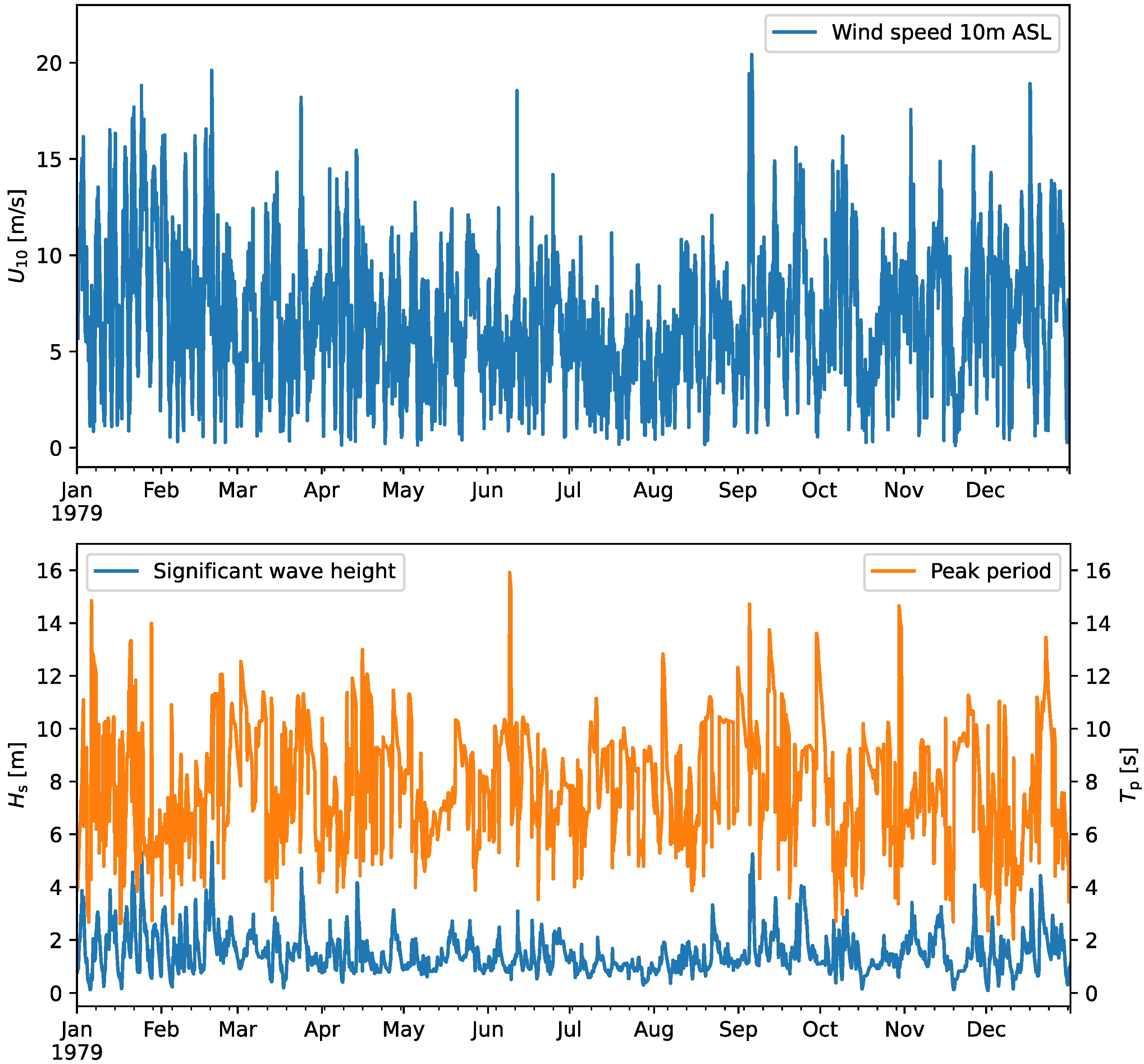
2.1. Historical Weather Data

The historical weather database employed for the analysis of this paper contained 40 years (1979–2018) of measured meteorological and oceanographic (metocean) data, in time steps of one hour. Although the measurements were taken over such a long time period, no trends related to a possible effect of the climate change were observed over the years. As a consequence, this phenomenon was not considered in this analysis.

The significant wave height H_s, the peak wave period T_p, the wind speed at a 10 m reference height U₁₀, and the current speed were recorded in this database. For the purpose of this work, only the wave and wind data were used.

Table 1. Main metocean data characteristics.

Parameter	Value
Mean annual significant wave height	1.520 m
Mean annual wind speed at 10 m ASL	6.837 m/s
Mean annual peak wave period	7.701 s

shows the essential characteristics of the metocean data set.

The measurements of the first year (1979) are visualised in Figure 1. It is observed that the wind speeds are generally higher in the winter months than in the summer, with values above 15 m/s being an exception. A similar trend can be observed for the wave height, where more extreme conditions occur regularly during the winter months.

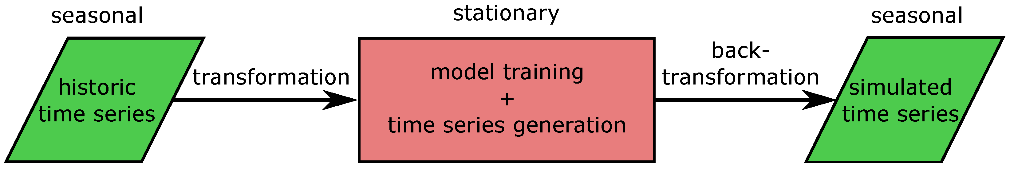
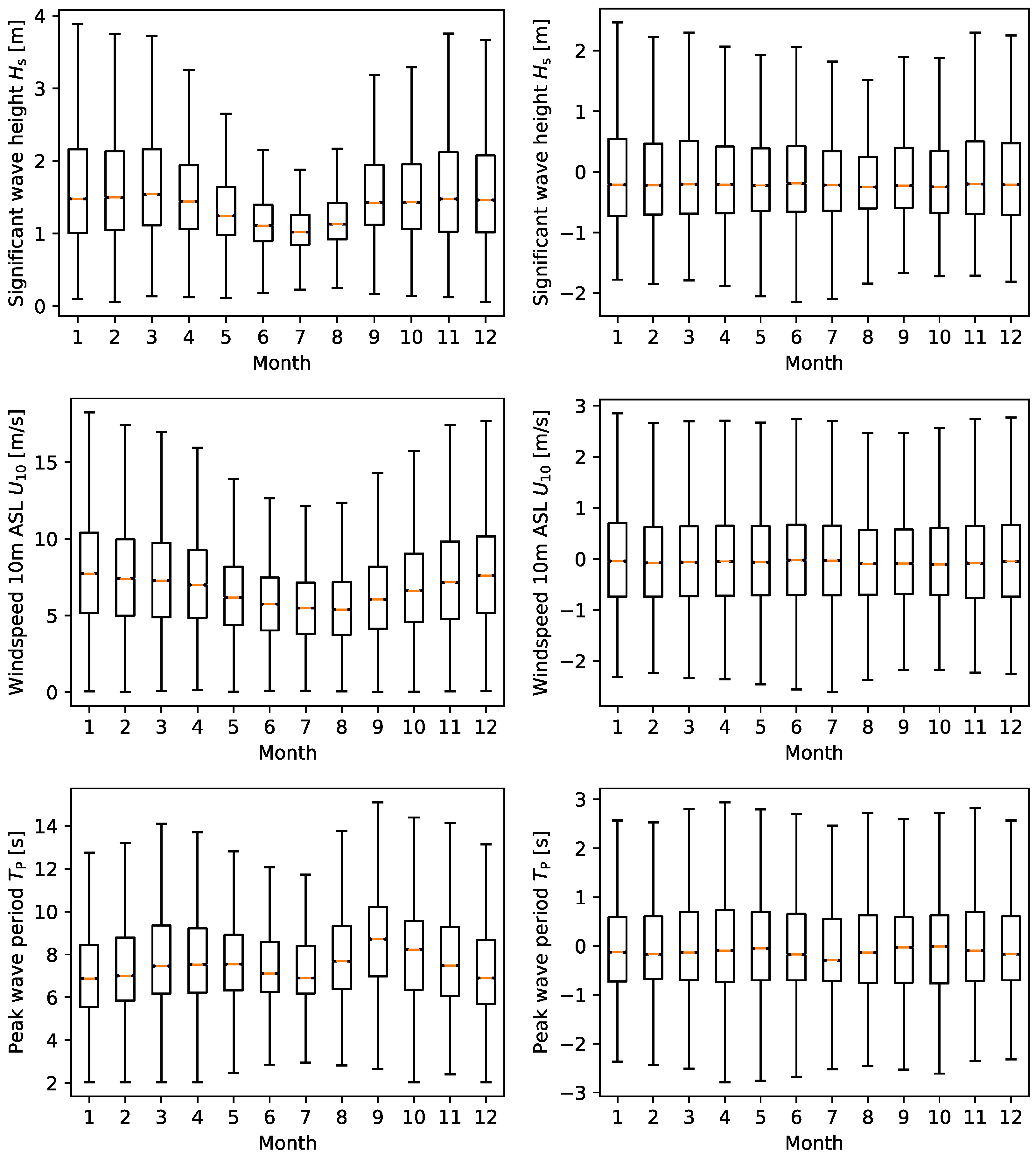
2.2. Data Processing

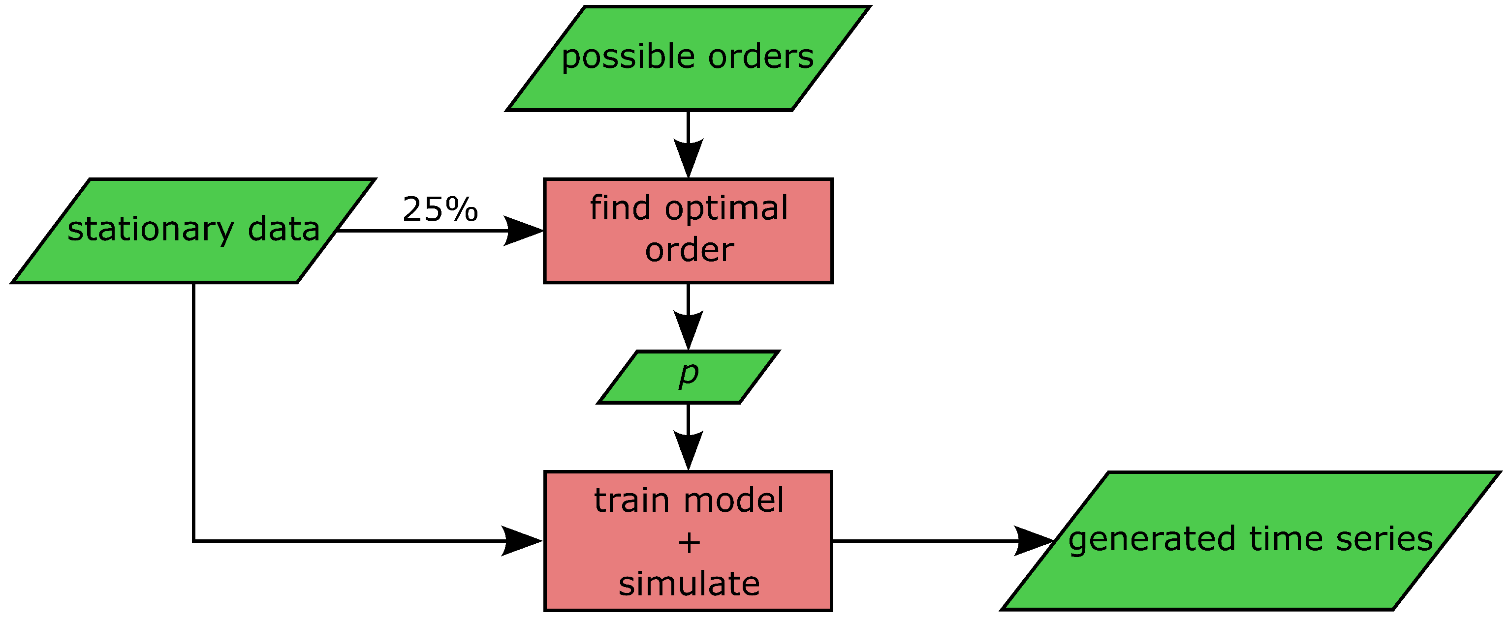
The measured time series contained some seasonal patterns. For instance, the wind speed varied between summer and winter (see Figure 1) and was also dependent on the time of day. The simulated data should include these trends. However, the algorithms used for their simulation cannot deal with this seasonality. To overcome this issue, the training data for the models were stationarised. As a consequence, the simulated time series of the models were also stationary and needed to be transformed back to be representative and deployed in a maintenance planning tool. This procedure is sketched in Figure 2.

To address this issue, several authors [9,11,17,19] suggested removing the seasonality by splitting the data into monthly sets. Besides neglecting the daily trends, this approach dramatically reduces the amount of training data. Alternatively, Soares and Cunha [16] applied a transformation based on a Fourier model fitted to the logarithmic time series of the monthly averages.

The approach adopted in this paper was similar to the one employed by Hagen et al. [17]. The univariate time series were standardised by using the mean ${\overline{X}}_{\mathrm{local},t}$ and standard deviation ${\widehat{\sigma }}_{\mathrm{local},t}$ over a selected range of days. This range was taken as ±15 days over the whole length of the time series. Hence, the two parameters ${\overline{X}}_{\mathrm{local},t}$ and ${\widehat{\sigma }}_{\mathrm{local},t}$ were estimated using $n\times 31$ values, where n is the length of the historic time series in years. The formula of this transform, from a time series $X_t$ to a stationary time series $\widetilde{X_t}$, is given by

$$\widetilde{X_t}=\frac{X_t-{\overline{X}}_{\mathrm{local},t}}{{\widehat{\sigma }}_{\mathrm{local},t}}.$$

(1)

By using this approach, it is easy to back-transform the data into time series containing a seasonality. Additionally, this standardisation method should be superior to the modification of the mean value suggested in [20], because both the mean value and the variance are under control. Furthermore, it avoids the problem of discontinuities between several month [17,20].

2.3. Markov Chain

This probabilistic model, named after Andrey Markov, has been widely used by researchers for several forecasting and simulation tasks [4,9,11,17,18,19,20]. The process to be modelled has to be discrete in time and switching between a finite number of states. The historic time series used in this analysis met the first requirement, being recorded in hourly measurements. Concerning the definition of a finite number of states, the approach followed in this paper was similar to the one in [17].

To derive the states $1,\cdots ,n$, the set of observations (H_s × U₁₀ × T_p) was partitioned in cuboids, which were numbered consecutively. The result was a discrete time series of scalar values, and thus the same theory as for a scalar-valued simulation was applied. To fit to different needs, the size of the cuboids can be varied. Therefore, if the behaviour of one parameter are sketched very roughly, the cuboids can be large along the corresponding axis. However, the number of states should be chosen carefully, as this highly affects the memory required.

The information on the states selected for this study are reported in

Table 2. Definition of the states for the Markov chain resulting in $n=15\times 20\times 15=4500$ states.

	Hs	U10	Tp
Min value	−1.2892	−1.7000	−1.6515
Number of states	15	20	15
Max value	2.5363	2.0940	2.2084

. The minimum and maximum values were chosen as the 2.5th and 97.5th percentile, respectively. The outlying 5% of the data were neglected to avoid creating states that were not important in the time series generation as they occurred very seldom.

For the purpose of the simulation, it is necessary that the transition probabilities only depend on the last p time steps of the time series $X_t$, with p indicating the order of the Markov chain. Given a time $t>p$ and states $a_1,\cdots ,a_t\in \{1,\cdots ,n\}$, the following equation applies

$$\mathbb{P}(X_t=a_t|X_{t-1}=a_{t-1},\cdots ,X_1=a_1)=\mathbb{P}(X_t=a_t|X_{t-1}=a_{t-1},\cdots ,X_{t-p}=a_{t-p}).$$

(2)

For $p=1$, Equation (2) is called the Markov property. Passing to a second-order Markov chain, the transition probabilities are abbreviated as follows

$$p_{a_1,a_2,a_3}:=\mathbb{P}(X_t=a_3|X_{t-1}=a_2,X_{t-2}=a_1).$$

To summarise these probabilities the transition matrix $\mathbf{A}$ is used

$$\mathbf{A}=\left(\begin{array}{cccc}{p}_{1,1,1}& p_{1,1,2}& \cdots & p_{1,1,n}\\ p_{1,2,1}& p_{1,2,2}& \cdots & p_{1,2,n}\\ ⋮& ⋮& \ddots & ⋮\\ p_{1,n,1}& p_{1,n,2}& \cdots & p_{1,n,n}\\ p_{2,1,1}& p_{2,1,2}& \cdots & p_{2,1,n}\\ p_{2,2,1}& p_{2,2,2}& \cdots & p_{2,2,n}\\ ⋮& ⋮& \ddots & ⋮\\ p_{n,n,1}& p_{n,n,2}& \cdots & p_{n,n,n}\end{array}\right)\in {\mathbb{R}}^{n^2\times n}.$$

(3)

Each row represents one combination of previous states, and its entries are the probabilities for the next time step. Thus, all rows of the transition matrix sum up to 1. The same scheme can be applied to Markov chains of any order.

The transition matrix is determined by counting the transitions between the states in the historic time series. In a first step, the number of transitions is set into the corresponding entry in the matrix. Then, the matrix is made right stochastic

$${\mathbf{A}}_{i,j}\leftarrow \left\{\begin{array}{cc}\frac{{\mathbf{A}}_{i,j}}{{\sum }_{m=0}^n{\mathbf{A}}_{i,m}},\hfill & \mathrm{if}\sum _{m=0}^n{\mathbf{A}}_{i,m}>0,\hfill \\ 1,\hfill & \mathrm{if}\sum _{m=0}^n{\mathbf{A}}_{i,m}=0\mathrm{and}{a}_p=j,\hfill \\ 0,\hfill & \mathrm{else}.\hfill \end{array}\right.$$

(4)

With states $a_1,\cdots ,a_p$ the matrix-row index i is given by

$$i=a_1{n}^p+a_2{n}^{p-1}+\cdots +a_p=\underset{modn=0}{\underbrace{(a_1{n}^{p-1}+a_2^{{}^p-2}+\cdots +a_{p-1})n}}+a_p.$$

(5)

Thus, the value of $a_p$ can be determined by $a_p=imodn$.

After extracting the behaviour of the time series in the transition matrix, the Markov chain can be used to simulate future values. The approach is similar to the one of [9,19,20]: given p previous time steps, the probability distribution for the next time step can be derived from the transition matrix. From there, one state is chosen randomly, but proportionally to its probability. This procedure can be repeated at each time step to simulate a time series of the desired length.

2.4. Vector Autoregressive Models

Autoregressive models are often used to model scalar-valued time series [4,21,22,23]. By following the approach of [24,25], it is possible to extend the theory to vector-valued time series, as has already been done by Soares and Cunha in [16]. A d-dimensional vector autoregressive time series ${\mathbf{X}}_t$ of order p (VAR(p)-process) is defined by

$${\mathbf{X}}_t={\mathsf{\Phi }}_1{\mathbf{X}}_{t-1}+{\mathsf{\Phi }}_2{\mathbf{X}}_{t-2}+\cdots +{\mathsf{\Phi }}_p{\mathbf{X}}_{t-p}+{\mathbf{Z}}_t.$$

(6)

Here, ${\mathsf{\Phi }}_i\in {\mathbb{R}}^{d\times d}$ for $i\in \{1,\dots ,p\}$ are the coefficient matrices and ${\mathbf{Z}}_t\in {\mathbb{R}}^d$ is a white noise vector, which is independent for different time steps, with a zero mean and a covariance matrix ${\sum }_{\mathbf{Z}}$.

Given a time series ${\mathbf{X}}_t$ and an order p, it is possible to estimate the coefficient matrices and the covariance matrix of the white noise by using a Yule–Walker estimator as in [25], Chapter 7.6.1. Alternatively, other approaches are suggested in [24], Chapter 3.

A very important aspect for the training of a VAR model is the appropriate selection of the order p. A VAR($p+1$)-process is always able to model a VAR(p) time series, but it is computationally more expensive than its lower-order replacement. Furthermore, there is a bigger stochastic uncertainty if more parameters need to be estimated. For this reason, some criteria are used to find a compromise between the goodness of fit and the value of the p, based on a penalty for the number of parameters used. In this work, the Hannan–Quinn criterion (HQ) from [24], Equation 4.3.8 was used, given by

$$\mathrm{HQ}\left(p\right)=\underset{\mathrm{goodness\; of\; fit}}{\underbrace{\ln \left(\det \left({\tilde{\sum }}_{\mathbf{Z}}\left(p\right)\right)\right)}}+\underset{\mathrm{penalty\; term}}{\underbrace{\frac{2\ln \ln T}{T}p{d}^2}},$$

(7)

where ${{\displaystyle \tilde{\sum }}}_{\mathbf{Z}}\left(p\right)$ is the maximum likelihood estimator of the white noise covariance matrix ${\sum }_{\mathbf{Z}}$, d is the dimension of the time series, and T is the number of training data. Other criteria are the final prediction error (FPE) [24], Equation 4.3.1 and the Akaike information criterion (AIC) [24], Equation 4.3.2. Both the AIC and the FPE tend to overestimate the order p for small time series dimensions ($d<5$) [24], Chapter 4.3.2. Another criterion, similar to the HQ, is the Schwarz criterion, [24], Equation 4.3.9, also known as the Bayesian information criterion (BIC). In

Table 3. VAR order selection based on some of the main criteria for autoregressive models. The minimum of each criterion is marked in green.

Order p	AIC	BIC	HQ
1	−73,961	−73,792	−73,909
2	−159,656	−159,403	−159,579
3	−170,549	−170,211	−170,446
4	−172,847	−172,425	−172,719
5	−173,016	−172,509	−172,861
6	−172,881	−172,290	−172,701
7	−173,919	−173,243	−173,713
8	−174,156	−173,396	−173,924
9	−174,171	−173,326	−173,913
10	−174,185	−173,257	−173,902
11	−174,212	−173,199	−173,903

, the AIC, HQ, and BIC were calculated for models of different order. For this comparison only one-fourth of the data were used to save on computational time.

The procedure around the VAR models is summarised in Figure 3. The flowchart can be seen as a detailed version of the middle box from Figure 2.

As for the Markov chain, presented in Section 2.3, the simulation of a time series via the VAR model follows an iterative approach. Given some starting values and a randomly generated white noise vector ${\mathbf{Z}}_t$, the first simulated value is derived, from which a second one can be computed, and so on. Because ${\mathbf{Z}}_t$ is regenerated every time, two simulations will be almost surely different.

The VAR models presented in this paper were implemented in Python 3 by using the statsmodels module [26].

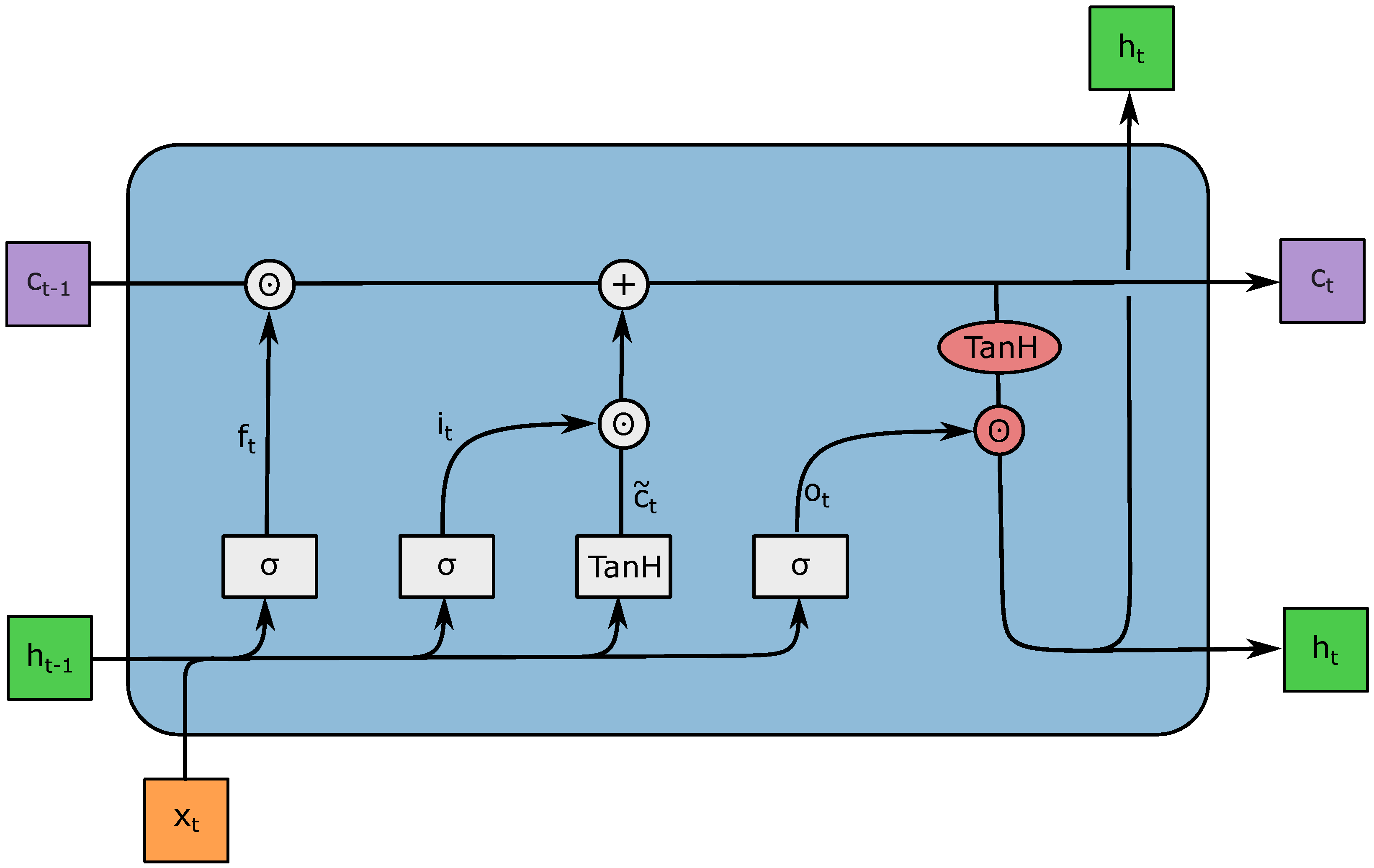
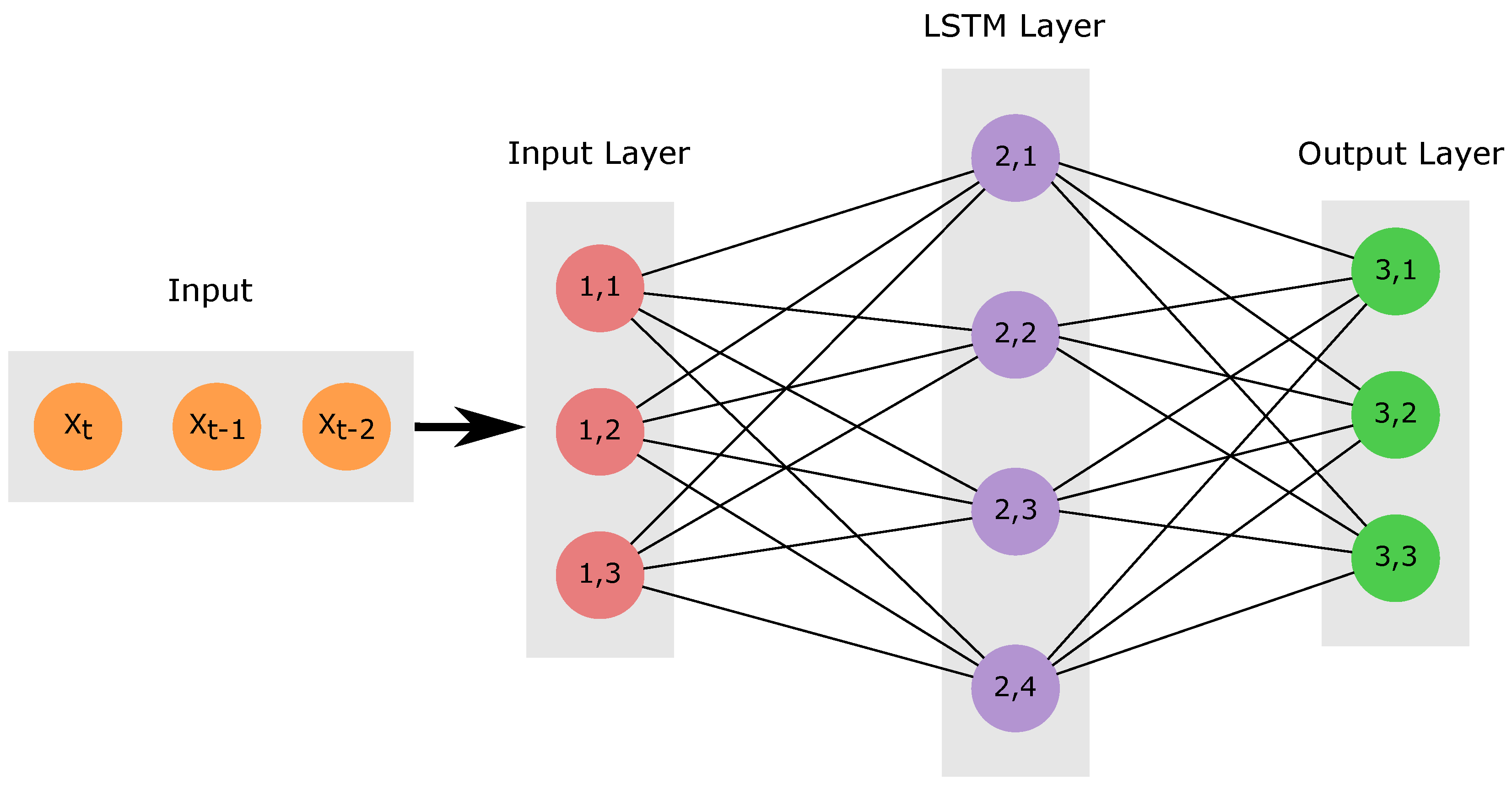
2.5. LSTM Neural Networks

The latest of the approaches presented in this paper is the long short-term memory (LSTM) neural network. This deep learning approach was developed by Hochreiter and Schmidhuber [27], and it has been widely used in context of time series, e.g., [11,21,23]. The LSTM networks are an enhanced version of recurrent neural networks (RNN) [28], Chapter 8, which in turn build up on multilayer perceptrons [28], Chapter 4. As indicated by their name, the advantage of LSTM networks over RNNs is in the long-term memory. Therefore, they were more suitable for this paper.

Figure 4 visualises a layer of the LSTM neural network, to help explain the way it works. For more details on the topic, the reader is referred to [29].

Starting from the outside of Figure 4, there are the input vector ${\mathbf{x}}_t$, the hidden state ${\mathbf{h}}_t$, which is also the output, and the cell state ${\mathbf{c}}_t$, which works as the long-term memory.

Furthermore, there are two activation functions in a LSTM layer: the sigmoid function $\sigma$ and the hyperbolic tangent TanH. These are applied component-wise to the corresponding vectors. In the blue box are three gates which perform the same task; they get multiplied to other vectors using the Hadamard product “⊙”, i.e., a component-wise multiplication of two vectors. Each gate is therefore used to control the amount of information that passes the “⊙”-multiplication. For this purpose, all three gates have their own weight matrices and bias vectors. In detail, the

• Forget gate${\mathbf{f}}_t$ controls how much of the old cell state ${\mathbf{c}}_{t-1}$ is forgotten for every component;
• Input gate${\mathbf{i}}_t$ determines which information from the current time step is important and should be added to ${\mathbf{c}}_t$;
• Output gate${\mathbf{o}}_t$ decides which information from ${\mathbf{c}}_t$ (activated with the TanH) should be saved in the hidden state ${\mathbf{h}}_t$.

To use this architecture for time series forecasting, the most common approach is to aim for ${\mathbf{x}}_{t+1}\approx {\mathbf{h}}_t$. This is achieved during a training phase, in which the neural network uses the training data for several epochs divided into batches. After the forecast for one batch, the errors are backpropagated, such that all the matrices and the bias vectors are updated to fit the LSTM network more and more to the training data.

Prior to the start of the training, some hyperparameter need to be defined. These are listed in

Table 4. Hyperparameter of the LSTM neural network.

Parameter	Value
Order	8
Input neurons	3
Neurons in LSTM layer	100
Output neurons	3
Optimiser	Adam
Loss function	MSE
Epochs	5
Batch size	500

, together with their values used.

The order of the model is defined as in Section 2.4. It determines how many time steps the LSTM network uses to train and simulate. An eighth-order model was chosen for consistency to the VAR(8)-model identified in Table 3. In this way, both approaches held the same amount of information.

Figure 5 shows the structure of the LSTM network used in this paper. Its implementation in Python 3 was obtained by using the Keras module [30].

The simulation of the time series with LSTM neural networks is received as for the VAR model. The noise is received from the errors the LSTM model makes on the training data in a separate run after the training. The distributions of these errors are saved independently per measurement, by making the assumption that the covariance matrix of the noise is a diagonal matrix. To simulate, the network is given some starting values based on which it predicts the next value, and finally adds the randomly generated noise. This procedure can be repeated to get an arbitrarily long time series.

2.6. Metrics for Joint Probability Density Functions

To compare the joint probability density functions (PDFs) of the different simulations later on in Section 3, we define several metrics in the following.

The Bhattacharyya coefficient (BC), introduced in [31], is calculated by

$$\mathrm{BC}(p,q)=\sum _{x\in X}\sqrt{p\left(x\right)q\left(x\right)},$$

(8)

where x are cuboids partitioning the multidimensional space X, which contains the measurements, while p and q are the relative frequencies of these cuboids. The more similar the distributions are, the larger the $\mathrm{BC}(p,q)$ becomes, in a range between 0 and 1.

As a second measure of similarity, the Kullback–Leibler divergence (${\mathrm{D}}_{\mathrm{KL}}$), introduced in [32], is defined as

$${\mathrm{D}}_{\mathrm{KL}}(p,q)=\sum _{x\in X}p\left(x\right)\ln \left(\frac{p\left(x\right)}{q\left(x\right)}\right).$$

(9)

The ${\mathrm{D}}_{\mathrm{KL}}$ is zero for identical joint PDFs and it cannot be negative. Therefore, the aim is to approach a ${\mathrm{D}}_{\mathrm{KL}}$ close to zero.

The Kullback–Leibler divergence is not symmetric, i.e., ${\mathrm{D}}_{\mathrm{KL}}(p,q)\ne {\mathrm{D}}_{\mathrm{KL}}(q,p)$, and it also accounts for the division by zero, which results into an infinite value of ${\mathrm{D}}_{\mathrm{KL}}$.

To cope with the limitations of the Kullback–Leibler divergence, the Jeffrey divergence ${\mathrm{D}}_{\mathrm{J}}$ was considered as well. This modified definition of the divergence is symmetric and also superior in other aspects [33]. It is calculated by

$${\mathrm{D}}_{\mathrm{J}}(p,q)=\sum _{x\in X}p\left(x\right)\ln \left(\frac{p\left(x\right)}{m\left(x\right)}\right)+q\left(x\right)\ln \left(\frac{q\left(x\right)}{m\left(x\right)}\right),$$

(10)

where $m\left(x\right)=\frac{p\left(x\right)+q\left(x\right)}{2}$.

Finally, another measure of the similarity of two PDFs is given by the histogram intersection (HI) [33], which indicates how much overlap there is between two distributions

$$\mathrm{HI}(p,q)=\sum _{x\in X}\min \{p\left(x\right),q\left(x\right)\}.$$

(11)

3. Results

After the models were trained on the full 40-year data set, we simulated 25 years of multivariate time series. Different metrics and statistics on these simulations are presented in this section. Special attention was given to comparing the results across the several models and investigate how they perform in comparison to the original data set. A first- and a second-order Markov chain, a VAR model, and an LSTM neural network were applied as explained in Section 2.

3.1. Preprocessing of the Data

The purpose of the standardisation is the removal of the seasonal influences. Hence, Figure 6 compares the training data of H_s, U₁₀ and T_p before (on the left) and after (on the right) the transformation. These boxplots are based on the whole data set divided into month, and they mark the median in orange.

A clear seasonal influence is visible in the boxplots of the measured data (on the left), especially for H_s and U₁₀. As it can be observed, on the right-hand side of Figure 6, the standardisation method is able to remove most of the seasonality effect from the data. Nevertheless, there are still differences in the distributions; the sizes of the boxes, marking the 25th and 75th percentiles, and the median are not equal for all months. However, as the approach only controls the mean value and the variance, these drawbacks were deemed acceptable.

Concerning the interconnection between the data over a large time period, Figure 7 shows how the autocorrelation functions developed over 36 months. This range was chosen to observe the similarities over multiple years. Although the transformation does not dramatically change the autocorrelation for any of the measurements, the standardised results (orange line) come very close to the desired outcome. Overall, the properties of the historic time series are homogenised across the several months, and it is thus reasonable to treat the standardised time series as stationary.

3.2. Single Measurements Comparison

In the following, the scalar-valued time series extracted from the vector-valued simulations are considered. Using these, there are several metrics to be evaluated and compared across the models.

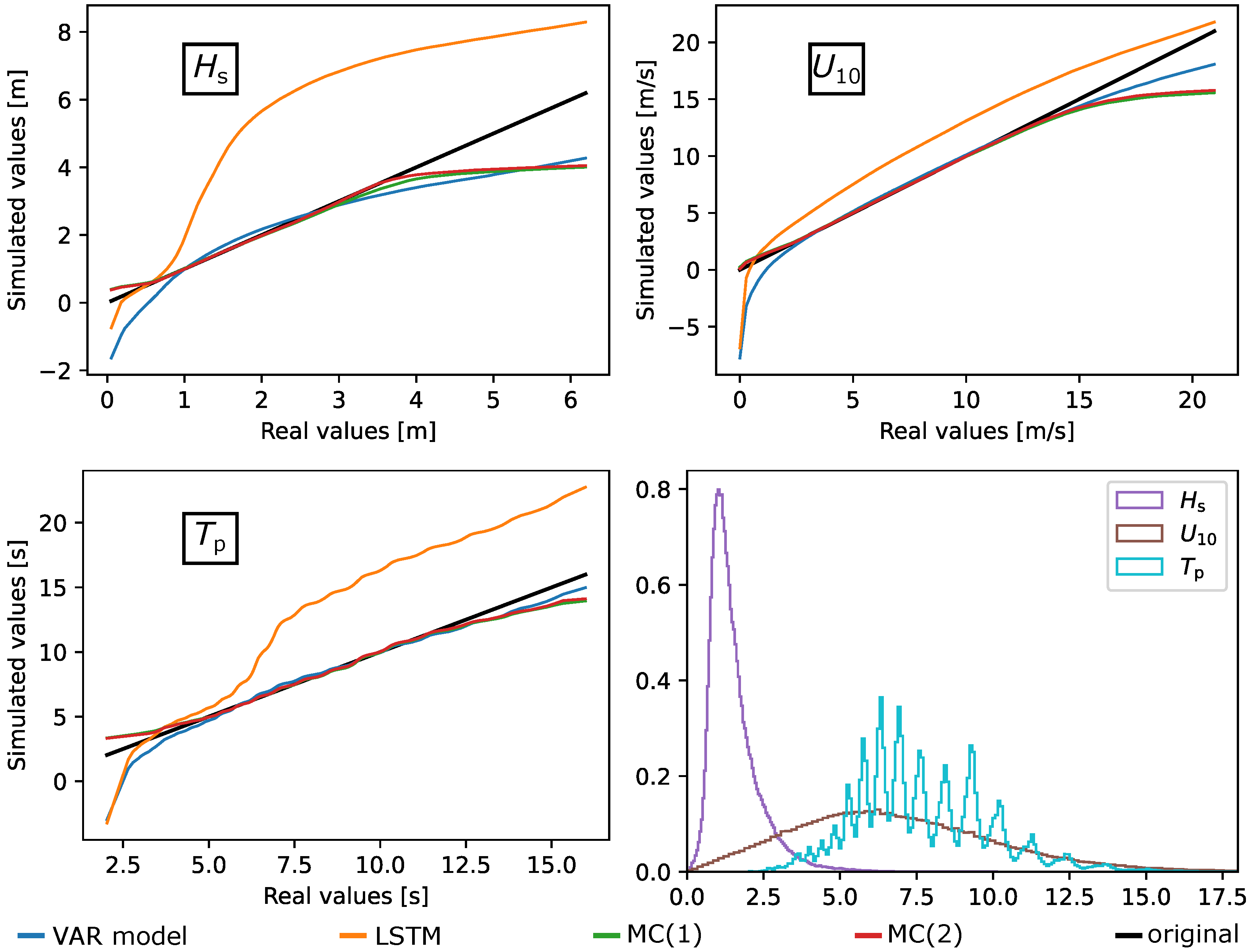
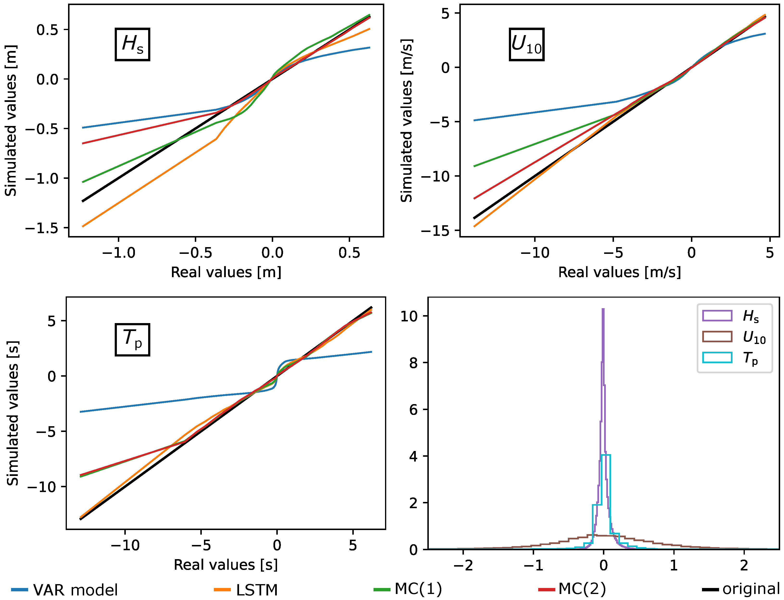
3.2.1. Marginal Distributions and Increments

The marginal distributions of the data, broken down into the different measurements, are reported in

Table 5. Different statistics on the simulations, taken before the back-transformation.

		VAR Model	LSTM	MC(1)	MC(2)	Original
Hs	mean	−0.0151	2.8167	−0.0287	−0.0484	−0.0022
	std	1.0073	2.4503	0.9036	0.8670	0.9948
	min	−4.3077	−2.6322	−1.2892	−1.2892	−2.2746
	25%	−0.6968	0.4199	−0.6867	−0.6854	−0.6652
	50%	−0.0139	3.3725	−0.2328	−0.2417	−0.2199
	75%	0.6671	4.8972	0.4139	0.4037	0.4186
	max	3.9227	8.3683	2.5363	2.5361	13.9059
U10	mean	−0.0020	0.8251	−0.0132	−0.0239	−0.0006
	std	1.0101	1.1068	0.9470	0.9285	0.9980
	min	−4.5885	−4.0388	−1.7000	−1.7000	−2.6080
	25%	−0.6838	0.0601	−0.7223	−0.7270	−0.7209
	50%	0.0003	0.8593	−0.0763	−0.0781	−0.0656
	75%	0.6786	1.5875	0.6315	0.6213	0.6369
	max	4.4298	5.8560	2.0940	2.0940	8.7361
Tp	mean	0.0018	1.9856	−0.0054	−0.0158	−0.0009
	std	0.9976	1.9515	0.9566	0.9287	0.9978
	min	−4.5479	−5.4943	−1.6515	−1.6514	−3.1213
	25%	−0.6751	0.1651	−0.7291	−0.7356	−0.7221
	50%	−0.0038	2.4620	−0.1392	−0.1299	−0.1337
	75%	0.6734	3.5614	0.6626	0.6380	0.6506
	max	4.6768	9.2085	2.2083	2.2084	5.4062

. This table compares the estimates, in the stationary state, across the several models and the original time series. The statistics of the 25-year simulations are provided in terms of the mean value, the standard deviation, and the percentiles of the different measurements.

Over all measurements, it can be observed that there is almost no correspondence between the results of the LSTM model and the original time series statistics. In contrast, the mean value and variance are adequately reproduced by the VAR model, while the Markov chains have a variance too small compared to that of the real data. Concerning the percentiles and the extrema, the VAR model generates approximately symmetric distributions. The Markov chains are instead able to replicate the asymmetry of the original data.

To better discuss the distributions of the simulated values, their quantile–quantile plots (QQ plots) are shown in Figure 8. If a simulated measurement has the same distribution as the original one, this is represented as a straight black line in the plots. The closer the simulations get to this straight line, the more accurate their marginal distributions are, see [34]. The bottom right plot of Figure 8 shows the distribution of the original data; the vertical axis is scaled so that the area below the histograms sums up to 1. The QQ plots confirm the speculations on the goodness of the LSTM model: it is evident that the yellow line completely differs from the trend wanted. As regards the VAR model, it can be seen that its lower quantiles reach very small and even negative values. This problem occurs due to the fact that the model cannot anticipate the natural limits of the measurements. A similar but slightly better performance is shown by both Markov chains. The difference in the higher and lower percentiles appears because the outlying values are neglected in the definition of the states (Section 2.3).

Another aspect to be investigated is the behaviour of the increments, defined as the differences between the values. The increments are analysed to see how much, and in which sense the values differ from the preceding ones. Once again, the QQ plots are used for this purpose (see Figure 9). In terms of increment, the VAR model performs worse than all the other algorithms. It tends to simulate too little increments across all the measurements. The increments of the LSTM model are distributed similarly to the ones of the original data, especially for the wind speed and the peak wave period. The Markov chains perform better than the VAR model, but worse than the LSTM model. It is worth noticing that the second-order Markov chain is a little more accurate than its first-order equivalent.

3.2.2. Earth Mover’s Distance

The earth mover’s distance (EMD) is calculated between two different distributions p and q. This measure quantifies how different these distributions are according to the following logic: it is imagined that both distributions are landscapes, and one is transformed into the other. The EMD assesses the amount of work to be done in terms of earth to be moved. Because the optimal flow has to be determined at first, this measure is not easy to derive for high-dimensional distributions. More information on this metric can be found in [33].

Table 6. Earth mover’s distances for the simulated values and the increments. The best result is marked in green.

		EMD of the Values $\times {10}^3$	EMD of the Increments $\times {10}^3$
	VAR model	0.3031	0.4160
HS	LSTM	1.0487	0.4219
	MC(1)	0.0797	0.5396
	MC(2)	0.0726	0.5363
	VAR model	0.0402	0.2877
U10	LSTM	0.1580	0.1089
	MC(1)	0.0577	0.1237
	MC(2)	0.0612	0.1276
Tp	VAR model	0.2255	1.2661
	LSTM	0.6922	0.8886
	MC(1)	0.2250	0.8730
	MC(2)	0.2377	0.8728

summarises the values of the EMDs for both the simulated values and the increments considered in Section 3.2.1. The values of the EMD were calculated using a normalised histogram with 1000 bins.

Using this metric, the results from Figure 8 and Figure 9 are put into perspective. The EMD is not too sensitive to the border areas since most of the values are concentrated in the middle. Therefore, the differences which appear large in the QQ plots can be compensated by moving a small amount of “earth”. The goodness of the simulations of the Markov chains does not stand out as in Figure 8 and Figure 9. However, it is worth recalling that these models are the only ones having no negative outliers, in contrast to the VAR and the LSTM models. Further weaknesses of the VAR model is in the distribution of the increments of the U₁₀ and the T_p measurements. The big offset in the distribution of the values simulated by the LSTM model can be noticed again in the EMD.

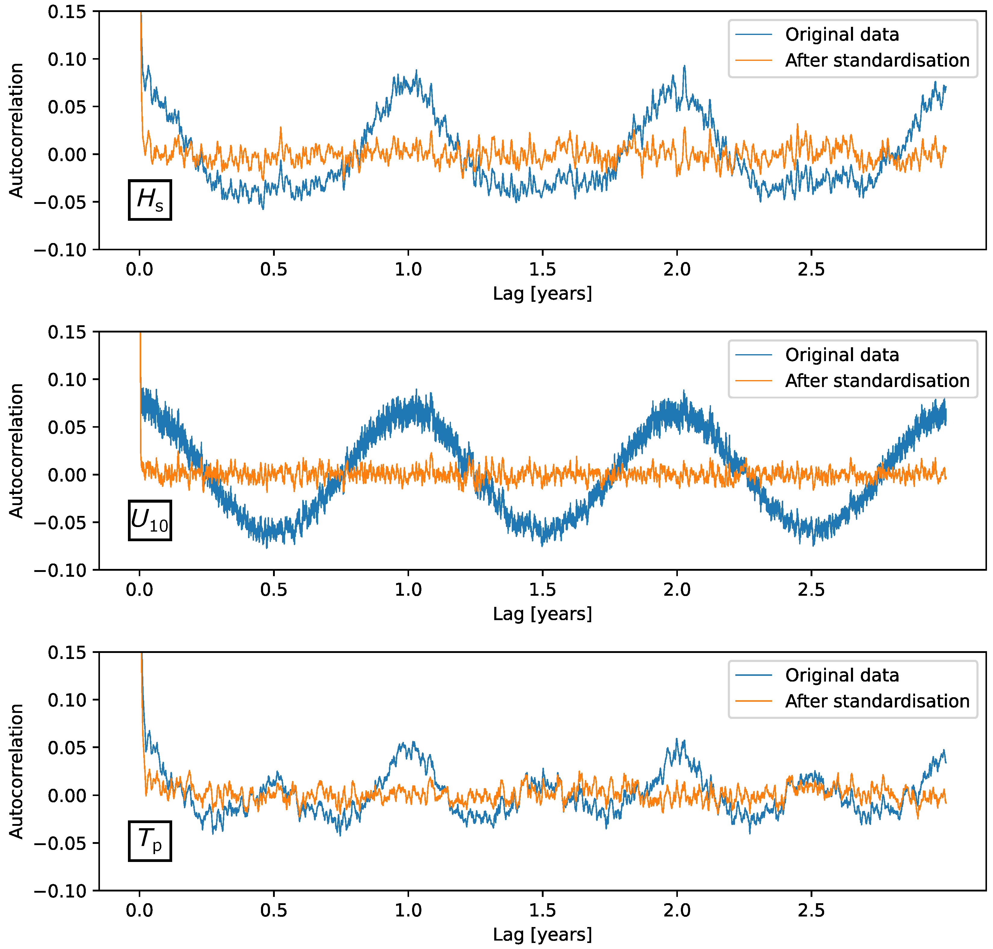
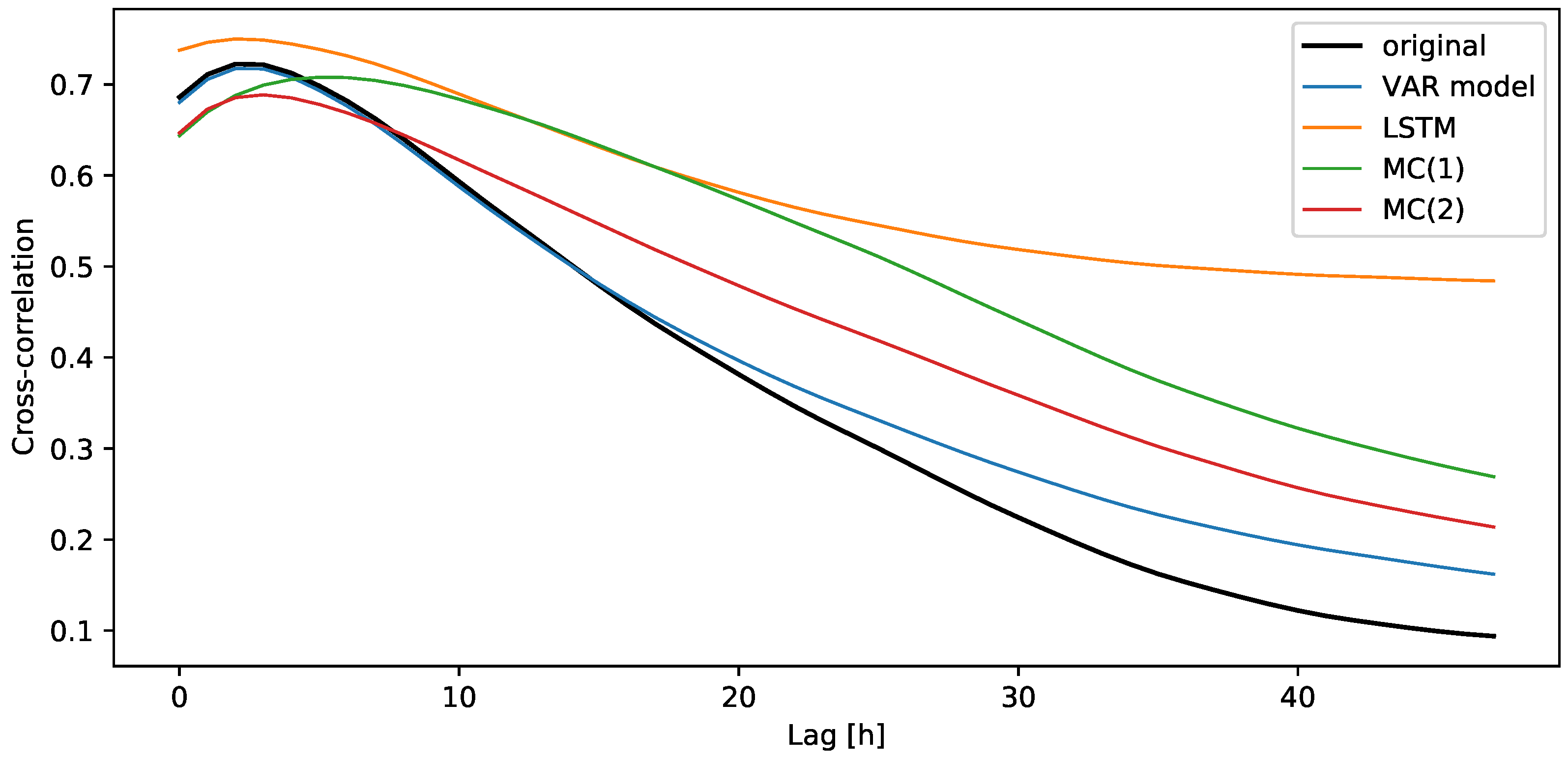
3.2.3. Autocorrelation

To analyse the interconnection between the time steps of the simulations, the autocorrelation was calculated as defined in [25], Chapter 3. Figure 10 shows the autocorrelation functions for the three measurements. For all measurements, the VAR model performs best. In contrast to the other models, the autocorrelation of the LSTM decreases too slowly. This is an indication for a strong connection between the corresponding time steps, which is much weaker in the original time series. The autocorrelation of the first-order Markov chain is always bigger than the one of the second-order model. This can be related to the fact that the first-order Markov chain cannot capture the tendencies in the simulated data, and thus it is prone to stay in the last state with a high probability. This phenomenon is already known, and it leads to a high autocorrelation [20].

3.3. Multidimensional Results Comparison

To conclude on the results section, a closer look is given to the interaction between the estimated measurements and their joint probability distributions.

3.3.1. Cross-Correlation of the Simulations

Similarly to the concept of the autocorrelation, it is possible to estimate a cross-correlation between two time series as their connection at different time steps. A definition can be found in [24], Equation 2.1.45. In Figure 11, the cross-correlations between the wave height and the wind speed are shown. The peak on the left shows that the wave height reacts to the wind speed, and their correlation reaches a maximum after about two hours. The VAR model shows accurate results again, nearly identical to the original time series for the first twelve hours. The LSTM model exhibits the same issues as for the autocorrelations (cf. Figure 10). The Markov chains’ estimates are closer to those of the original time series, with a clear advantage of the second-order Markov chain over the first one.

3.3.2. Joint Probability Density Functions

This section compares the simulated joint probability density functions (joint PDFs) to the original ones. Because a visualisation of the three-dimensional distributions is not feasible, several metrics were introduced in Section 2.6. In

Table 7. Comparison of the simulated joint PDFs; the best result is marked in green.

	BC	${\mathbf{D}}_{\mathbf{KL}}$	${\mathbf{D}}_{\mathbf{J}}$	HI
VAR model	0.1141	∞	1.2496	0.0594
LSTM	0.1918	∞	1.1545	0.1034
MC(1)	0.4082	∞	0.8840	0.2305
MC(2)	0.4163	∞	0.8735	0.2359

, these criteria were used once again to compare and discuss the different simulation models. The histograms, to calculate the characteristic criteria of the joint PDFs, were created by using $100\times 100\times 100$ cuboids.

The Kullback–Leibler divergence is infinite for all the models, meaning that there are cuboids having a positive probability in the historic data, and these do not appear in the simulations. Across all the other metrics, the second-order Markov chain behaves the best, closely followed by its first-order equivalent. On the other hand, the VAR model performs the worst, being even inferior to the LSTM model.

4. Discussion

Starting with the preprocessing of the data, presented in Section 3.1, a standardisation approach was used to make the simulations independent from the seasonality of the historic data. Figure 6 and Figure 7 proved the achievement of stationary time series, by maintaining a similar distribution of the data and attaining a constant autocorrelation. Because of the switch from monthly based to daily based time frames, this approach can be considered superior to the procedures generally used in the literature [17,20].

Several data analysis visuals and metrics were deployed to discuss the performance of the different stochastic weather generators and come to a comprehensive conclusion. The LSTM model was seen to perform poorly across every stage of the analysis, with the exception of the increments of Figure 9. In terms of predictions, they have been shown to outperform the autoregressive models [21,23]. However, this did not seem to hold for the simulation purpose. This discrepancy might be associated to the approach adopted for the inclusion of the independent noise, which was integrated to add some randomness to the simulation process. The VAR model delivered a very accurate mean and standard deviation, but it was not able to preserve the asymmetric distribution (see Table 5). Additionally, its symmetric marginal distribution fell in the negative range after the back-transformation. To solve this problem a postprocessing of the simulation could be used to fit the marginal distribution to the one of the historic time series. By contrast, both Markov chains were able to keep the asymmetry of the historic data and match their marginal distributions very well.

Concerning the increments, the Markov chains were superior to the VAR model, which simulated too small increments. The increments of the VAR model were partly consisting of the noise vector ${\mathbf{Z}}_t$. During the training phase, the model minimised the standard deviation of the noise to deliver a good fit to the training data. It also might be that the VAR model fitted the data too well, and therefore the noise had a too small variance. As regards the correlation functions from Figure 10 and Figure 11, the VAR model outperformed the Markov chains. This can be explained by the fact that the VAR model is structured into matrices and takes into account the relation with eight time steps. On the other hand, the Markov chains consider only the relationship with one to two time steps. The second-order Markov chain can access a higher level of information from the original data, and thus it showed better a cross-correlation of wind speed U₁₀ and significant wave height H_s. Regarding the joint PDFs, the simulations of the VAR model performed generally worse than the ones of the Markov chains. This might be related to the presence of negative values in the VAR simulations, which did not intersect with the histogram of the original data.

5. Conclusions and Future Work

The aim of this paper was to benchmark the goodness of the simulation of vector-valued time series against different stochastic weather generators. Markov chains were used to simulate vector-valued time series by following a similar approach to [17]. The novelty of this approach was to combine the multivariate and second-order Markov chain in the field of offshore weather time series. The simulation results from this model were judged to be among the best, especially in terms of their correlation metrics. Among the other statistics derived, the first-order Markov chain did not differ significantly in its results and is thus worth being considered to save on computational time. Another type of simulation models considered in this analysis was the vector autoregressive (VAR), which was implemented as in [16,22]. The results of the VAR models were shown to be very accurate in obtaining the time series correlation and standard deviation. In turn, they were assessed to be weaker than the Markov chains with regards to the probability distributions. Finally, a long short-term memory (LSTM) neural network was deployed similar to [11]. The novelty was to use it for offshore weather time series simulations by including a random noise. Despite the successful training of a LSTM neural network on the historical data, this particular set up of the model is not recommended for time series simulation, due to the poor results shown across most of the statistics derived.

Some aspects can be still improved in the setup of these models, as none of them managed to perfectly reproduce the information held in the original time series. As regards the use of LSTM networks for time series simulation, the approach might need to be refined. The training phase does not prepare the network properly for the long-term simulations. Furthermore, the randomness of the noise can be integrated in several ways, potentially leading to better results.

The weaknesses of the VAR model concern the representation of the increments. Additionally, its simulated values fall into the negative sphere due to the approach used in the generation of the noise vector ${\mathbf{Z}}_t$. If the noise generation is regulated by the simulations, instead of being modelled independently, unrealistic large or small values can be avoided. This change can also lead to improvements of the joint probability density functions. However, it should be avoided that this enhancement is achieved at the cost of the other time series’ statistics.

The simulations of Markov chains are typically not smooth because they output a uniformly distributed random number in the simulated bin. This can be regulated by using a smoothing filter as in [20]. Other approaches that can be used to better represent the probabilities involve the increase of the Markov chain order and the number of states. Both these solutions come at the cost of computational time, and they require a larger set of training data to approximate the transition probabilities well. Thus, to tackle the fine-tuning of a Markov chain, the optimal solution should be found by compromising on all these aspects.

References

1. EU. Directive (EU) 2018/2001 of the European Parliament and of the Council on the Promotion of the Use of Energy from Renewable Sources; EU: Brussels, Belgium, 2018. [Google Scholar]
2. Bundesverband-WindEnergie. Europa in Zahlen. 2022. Available online: https://www.wind-energie.de/themen/zahlen-und-fakten/europa/#:~:text=Windenergie%20in%20Europa&text=Mit%20458%20TWh%20produziertem%20Strom,und%20Gro%C3%9Fbritannien%20mit%2024%20GW (accessed on 26 April 2022).
3. Johnston, B.; Foley, A.; Doran, J.; Littler, T. Levelised cost of energy, A challenge for offshore wind. Renew. Energy 2020, 160, 876–885. [Google Scholar] [CrossRef]
4. Seyr, H.; Muskulus, M. Decision Support Models for Operations and Maintenance for Offshore Wind Farms: A Review. Appl. Sci. 2019, 9, 278. [Google Scholar] [CrossRef] [Green Version]
5. Graham, C. The parameterisation and prediction of wave height and wind speed persistence statistics for oil industry operational planning purposes. Coast. Eng. 1982, 6, 303–329. [Google Scholar] [CrossRef]
6. Brokish, K.; Kirtley, J. Pitfalls of modeling wind power using Markov chains. In Proceedings of the 2009 IEEE/PES Power Systems Conference and Exposition, PSCE, Seattle, WA, USA, 15–18 March 2009; pp. 1–6. [Google Scholar] [CrossRef]
7. Ailliot, P.; Monbet, V. Markov-switching autoregressive models for wind time series. Environ. Model. Softw. 2012, 30, 92–101. [Google Scholar] [CrossRef] [Green Version]
8. Wang, X.; Guo, P.; Huang, X. A Review of Wind Power Forecasting Models. Energy Procedia 2011, 12, 770–778. [Google Scholar] [CrossRef] [Green Version]
9. Scheu, M. Maintenance Strategies for Large Offshore Wind Farms. Energy Procedia 2012, 24, 281–288. [Google Scholar] [CrossRef] [Green Version]
10. Seyr, H.; Muskulus, M. Using a Langevin model for the simulation of environmental conditions in an offshore wind farm. J. Phys. Conf. Ser. 2018, 1104, 012023. [Google Scholar] [CrossRef]
11. Pandit, R.; Kolios, A.; Infield, D. Data-Driven weather forecasting models performance comparison for improving offshore wind turbine availability and maintenance. IET Renew. Power Gener. 2020, 14, 2386–2394. [Google Scholar] [CrossRef]
12. BMU (Bundesministerium fuer Umwelt, Federal Ministry for the Environment, Nature Conservation and Nuclear Safety); Project Executing Organisation; PTJ (Projekttraeger Juelich). FINO3 Metrological Masts Datasets. Available online: https://www.fino3.de/en/ (accessed on 26 April 2022).
13. Skobiej, B.; Niemi, A. Validation of copula-based weather generator for maintenance model of offshore wind farm. WMU J. Marit. Aff. 2022, 21, 73–87. [Google Scholar] [CrossRef]
14. Niemi, A.; Torres, F.S. Application of synthetic weather time series based on four-dimensional copula for modeling of maritime operations. In Proceedings of the Oceans Conference Record (IEEE), MTS, San Diego, CA, USA, 20–23 September 2021. [Google Scholar] [CrossRef]
15. MIT Data To AI Lab. Copulas Python Library; MIT Data To AI Lab: Cambridge, MA, USA, 2018. [Google Scholar]
16. Soares, C.G.; Cunha, C. Bivariate autoregressive models for the time series of significant wave height and mean period. Coast. Eng. 2000, 40, 297–311. [Google Scholar] [CrossRef]
17. Hagen, B.; Simonsen, I.; Hofmann, M.; Muskulus, M. A multivariate Markov Weather Model for O&M Simulation of Offshore Wind Parks. Energy Procedia 2013, 35, 137–147. [Google Scholar] [CrossRef] [Green Version]
18. Guo, S.; Liu, C.; Guo, Z.; Feng, Y.; Hong, F.; Huang, H. Trajectory Prediction for Ocean Vessels Base on K-order Multivariate Markov Chain. In Wireless Algorithms, Systems, and Applications; Chellappan, S., Cheng, W., Li, W., Eds.; Springer International Publishing: Cham, Switzerland, 2018; pp. 140–150. [Google Scholar] [CrossRef]
19. Nfaoui, H.; Essiarab, H.; Sayigh, A. A stochastic Markov chain model for simulating wind speed time series at Tangiers, Morocco. Renew. Energy 2004, 29, 1407–1418. [Google Scholar] [CrossRef]
20. Pesch, T.; Schröders, S.; Allelein, H.J.; Hake, J.F. A new Markov-chain-related statistical approach for modelling synthetic wind power time series. New J. Phys. 2015, 17, 055001. [Google Scholar] [CrossRef]
21. Siami-Namini, S.; Tavakoli, N.; Namin, A.S. A Comparison of ARIMA and LSTM in Forecasting Time Series. In Proceedings of the 2018 17th IEEE International Conference on Machine Learning and Applications (ICMLA), IEEE, Orlando, FL, USA, 17–20 December 2018. [Google Scholar] [CrossRef]
22. Dinwoodie, I.; Quail, F.; Mcmillan, D. Analysis of Offshore Wind Turbine Operation & Maintenance Using a Novel Time Domain Meteo-Ocean Modeling Approach. Turbo Expo Power Land Sea Air 2012, 6, 847–857. [Google Scholar] [CrossRef] [Green Version]
23. Dostal, L.; Grossert, H.; Duecker, D.A.; Grube, M.; Kreuter, D.C.; Sandmann, K.; Zillmann, B.; Seifried, R. Predictability of Vibration Loads From Experimental Data by Means of Reduced Vehicle Models and Machine Learning. IEEE Access 2020, 8, 177180–177194. [Google Scholar] [CrossRef]
24. Lütkepohl, H. New Introduction to Multiple Time Series Analysis; Springer Science & Business Media: Berlin/Heidelberg, Germany, 2005. [Google Scholar] [CrossRef]
25. Brockwell, P.; Davis, R. An Introduction to Time Series and Forecasting; Springer: Berlin/Heidelberg, Germany, 2002; Volume 39. [Google Scholar] [CrossRef] [Green Version]
26. Seabold, S.; Perktold, J. Statsmodels: Econometric and statistical modeling with python. In Proceedings of the 9th Python in Science Conference, Austin, TX, USA, 28 June–3 July 2010. [Google Scholar]
27. Hochreiter, S.; Schmidhuber, J. Long Short-Term Memory. Neural Comput. 1997, 9, 1735–1780. [Google Scholar] [CrossRef]
28. Zhang, A.; Lipton, Z.C.; Li, M.; Smola, A.J. Dive into Deep Learning. arXiv 2021, arXiv:2106.11342. [Google Scholar]
29. Olah, C. Understanding LSTM Networks. 2015. Available online: https://colah.github.io/posts/2015-08-Understanding-LSTMs/ (accessed on 15 April 2022).
30. Chollet, F. Keras. 2015. Available online: https://keras.io (accessed on 18 April 2022).
31. Bhattacharyya, A. On a Measure of Divergence between Two Multinomial Populations. Sankhyā Indian J. Stat. 1946, 7, 401–406. [Google Scholar]
32. Kullback, S.; Leibler, R.A. On Information and Sufficiency. Ann. Math. Stat. 1951, 22, 79–86. [Google Scholar] [CrossRef]
33. Rubner, Y.; Tomasi, C.; Guibas, L.J. The earth mover’s distance as a metric for image retrieval. Int. J. Comput. Vis. 2000, 40, 99–121. [Google Scholar] [CrossRef]
34. Marden, J.I. Positions and QQ Plots. Stat. Sci. 2004, 19, 606–614. [Google Scholar] [CrossRef]
Figure 1. The first year of weather measurements. At the top, the wind speed at reference height (U10). At the bottom, the wave characteristic parameter: the significant height (Hs) and the peak period (Tp).
Wind 02 00021 g001
Figure 2. The procedure of simulating time series in this paper.
Wind 02 00021 g002
Figure 3. Flowchart for the VAR model used in this work.
Wind 02 00021 g003
Figure 4. Schematic illustration of an LSTM Layer, adapted from [29].
Wind 02 00021 g004
Figure 5. Structure of an LSTM for a three-dimensional time series with four neurons in the LSTM layer.
Wind 02 00021 g005
Figure 6. Boxplots of the data split up into different months. On the left, the original data, which have been measured. On the right, the data after the standardisation.
Wind 02 00021 g006
Figure 7. The autocorrelation of the data before and after the standardisation.
Wind 02 00021 g007
Figure 8. QQ plots of the simulated values. Bottom right: distributions of the historical data.
Wind 02 00021 g008
Figure 9. QQ plots of the simulated increments. Bottom right: distributions of the increments from historical data.
Wind 02 00021 g009
Figure 10. The autocorrelation of the different simulations in comparison to the autocorrelation of the original time series.
Wind 02 00021 g010
Figure 11. The cross-correlation of Hs and U10 for the original time series and different simulations.
Wind 02 00021 g011