Wind Loading of Photovoltaic Panels Installed on Hip Roofs of Rectangular and L-Shaped Low-Rise Buildings

Abstract

Many residential houses in Japan have hip roofs with pitches ranging from 20° to 30°. Recently, roof-mounted photovoltaic (PV) panels have become popular all over the world for environmental conservation. The design of PV systems in Japan is usually based on the Japanese Industrial Standard (JIS) C 8955 (2017). However, the standard does not provide wind force coefficients for PV panels installed near roof edges (up to 0.3 m from the edge) because flow separation at the roof edges causes large up-lift forces on such panels. In this paper, we investigated the wind force coefficients for designing PV panels installed on hip roofs of rectangular and L-shaped low-rise buildings. The roof pitch was set to 25° as a typical value. Rectangular panels were installed almost over the whole roof, including the edge zones. Because the thickness of PV panels and the distance between PV panels and the roof are both as small as several centimeters, it is difficult to make wind tunnel models of PV systems with the same geometric scale as that for buildings. We focused on a numerical simulation using the unsteady Bernoulli equation to estimate the pressures in the space between PV panels and the roof. In the simulation, we used the time histories of wind pressure coefficients on the bare roof, which were measured in a turbulent boundary layer. We propose installing PV panels with small gaps between them along their short sides. The gaps may reduce the wind loads not only on the PV panels but also on the roofing due to pressure equalization. We discuss the optimum gap width from the viewpoint of wind load reduction.

1. Introduction

The objective of the present study is to provide useful information about the wind force coefficients of PV panels installed on hip roofs of practical residential houses. Furthermore, the effects of horizontal gaps between PV panels on the wind load reduction of both PV panels and roof cladding are investigated. For this purpose, a numerical simulation based on the unsteady Bernoulli equation is employed.

In recent years, solar energy has been exploited by installing photovoltaic (PV) systems on the roofs of buildings all over the world, considering the environmental conservation. In Japan, installing PV panels at a tilt angle of 20° to 30° against the horizontal plane is the most efficient from the viewpoint of power generation. Furthermore, hip roofs with pitches ranging from 20° to 30° are widely used for low-rise buildings, especially for residential houses. Hence, many PV panels are installed on hip roofs, as shown in Figure 1. In Japan, the structural design of PV systems is usually based on the Japanese Industrial Standard (JIS) C 8955 [1]. The standard provides positive and negative wind force coefficients for designing PV panels installed on sloped roofs as a function of roof pitch, β. However, it does not specify the values for panels installed near the eaves and ridges, up to 0.3 m from the edges, because the flow separation at the roof edges generates large up-lift forces on the panels. Therefore, PV panels are usually set at least 0.3 m back from the edges (see Figure 1). On the other hand, there is a demand to install PV panels on the whole roof area, including the edge zones, to maximize the total amount of electric power obtained from a building. In such a case, the wind loads on PV panels should be estimated appropriately, usually by employing a wind tunnel experiment. At present, little information is available for wind loading of PV panels installed on hip roofs, particularly near the edges.

Many researchers have investigated the wind loading of PV panels mounted on flat roofs [2,3,4,5,6,7,8,9,10,11,12,13]. The effects of tilt angle and location of PV panels, as well as the building geometry, on the wind loading of PV panels were investigated by many researchers based on wind tunnel experiments and/or CFD simulations. By comparison, the number of studies on PV panels mounted on sloped roofs is rather limited. Geurts and Blackmore [14] carried out a full-scale measurement and a wind tunnel experiment to measure the up-lift wind forces acting on a stand-off PV system mounted on a house, the roof pitch of which was β = 42°. The wind tunnel model of the PV panel had a plane dimension of 10 mm × 15 mm and a thickness of t_panel = 2 mm; the geometric scale, λ_L, of the model was 1/100. The clearance, H_panel, between the panel’s underside and the roof surface was varied from 0.25 to 3 mm in the experiment. The results indicated that the net wind forces on the PV panel were not significantly affected by H_panel. This feature may be related to the fact that the roof pitch was as high as 42°. Aly and Bitsuamlak [15] experimentally investigated the wind forces on PV panels mounted parallel to gable roofs of residential houses; the roof pitches were 14° and 22.6°, and the geometric scale of the wind tunnel models was 1/15. Three sizes of PV panels (small, medium and large) were tested. The value of H_panel was fixed to about 0.15 m at full scale. It was found that the wind load on individual panels was strongly dependent not only on the roof pitch, β, but also on the location and dimensions of the panel. Aly and Bitsuamlak recommended avoiding mounting PV panels near roof edges because large up-lift forces would be generated on the panels. Stenabough et al. [16] carried out a wind tunnel experiment to measure wind forces on PV panels mounted parallel to the gable roof (β = 30°) of a low-rise building. The full-scale dimensions of the tested panels were 50 cm wide and 145.5 cm long. The geometric scale of the wind tunnel models was 1/20, and the thickness, t_panel, was 3 mm (6 cm at full scale). The researchers focused on the effects of the horizontal gap width, G, between PV panels and the clearance, H_panel, on the net wind loads of PV panels. The values of G and H_panel were varied from 0 to 12 cm and from 0 to 20 cm at full scale, respectively. It was found that the net wind loads on PV panels decreased with an increase in G and/or with a decrease in H_panel. Such a wind load reduction is thought to be due to pressure equalization. Leitch et al. [17] measured the net wind forces on PV panels mounted parallel to gable roofs (β = 7.5°, 15°, 22.5°) of domestic buildings and the wind pressures on the underlying roof surface in a wind tunnel. The geometric scale of the wind tunnel models was 1/20. An array consisting of seven panels (1.0 m wide and 7.0 m long at full scale) was arranged at one of two positions on the roof. The thickness, t_panel, was 6 mm (120 mm at full scale), and the clearance, H_panel, was either 5 mm or 10 mm (100 mm or 200 mm at full scale). The aerodynamic shape factors for different array positions and roof pitches were provided. An interesting finding is that the maximum and minimum peak pressures on the roof were close to those on the bottom surface of the panel. Naeiji et al. [18] investigated the net wind forces of PV panels mounted on flat, gable and hip roofs. They used large models with a geometric scale of 1/6 in a large wind tunnel at Florida International University. The PV panel was 2 m in length, 1 m in width and 0.15 m in thickness at full scale. The effects of building height, H, panel clearance, H_panel, and panel tilt angle, β_panel, on the panel wind loads were investigated. It should be mentioned that the angle, β_panel, did not necessarily coincide with the roof pitch, β. The clearance, H_panel, tested was 0.3 m or 0.45 m at full scale, which was much larger than practical values. Takamori et al. [19] measured the wind forces on PV panels mounted parallel to gable roofs of low-rise buildings using 1/30 scale models. The thickness, t_panel, was 3 mm (90 mm at full scale). The panels were installed with no horizontal gap (i.e., G = 0 mm). The clearance, H_panel, and the roof pitch, β, were varied from 30 mm to 150 mm at full scale and from 10° to 40°, respectively. The wind pressure on the PV panels’ bottom surface was replaced by that on the underlying roof surface. This method is thought to be reasonable, judging from the above-mentioned findings of Leitch et al. [17]. The specifications of wind loads in JIS C 8955 [1] are mainly based on a study by Takamori et al.

In addition to the above-mentioned wind tunnel studies, several studies using CFD simulations have been carried out in recent years. Agarwall et al. [20] computed the wind pressures on PV arrays installed on industrial buildings with saw-type roofs with β = 20°, 30° and 40°. Li et al. [21] computed wind pressure distributions on PV arrays mounted on a hip roof. The tilt angle of PV panels with respect to the roof surface was varied from 2° to 30°; that is, the PV panels were not mounted parallel to the roof. Both studies used the Reynolds-averaged Navier–Stokes (RANS) turbulence models. Therefore, only the time-averaged wind pressure coefficients were obtained in these studies. In the structural design of PV systems, the maximum and minimum peak wind force coefficients on PV panels are required. For this purpose, a large eddy simulation (LES) is required. However, the computation loads required for LES are much larger than that for RANS. Furthermore, high-spec computers are necessary. In conclusion, few studies (either experimental or numerical) have been conducted on the wind loading of PV panels installed parallel to hip roofs of low-rise buildings, considering the dynamic load effects of fluctuating wind pressures. More information is necessary to appropriately evaluate the wind force coefficients of such PV panels, particularly for those placed near roof edges.

At present, wind tunnel experimentation is thought to be the most reliable method for estimating wind loads on buildings and structures. Regarding PV panels mounted on the roofs of low-rise buildings, the values of t_panel and H_panel are both as small as several centimeters (see Figure 1). Furthermore, to accurately obtain the net wind pressures on PV panels, it is necessary to install pressure taps on both the top and bottom surfaces of the model. Generally speaking, making wind tunnel models of PV panels with the same geometric scale as that for buildings (e.g., 1/100) is quite difficult. Therefore, it is necessary to use deformed models of PV panels in wind tunnel experiments [19], which may significantly affect the wind pressure distributions on the PV panels. Thus, we proposed a numerical simulation using the unsteady Bernoulli equation to estimate the pressure in the space between PV panels and the roof, which is called ‘layer pressure’ [22,23]. In the numerical simulation, we used the time histories of external pressure coefficients on the roof without PV panels (bare roof), which had been obtained from a wind tunnel experiment. It was confirmed that this simulation method could be used effectively to estimate the wind loads on PV panels, provided that t_panel and H_panel were both as small as several centimeters. Therefore, we applied this simulation method to the wind load estimation of PV panels mounted on hip roofs of residential houses with rectangular and L-shaped plans, which are widely used in Japan. The roof pitch was fixed to 25° as a representative value for residential houses. PV panels installed in the edge zones were also considered. We propose to install PV panels with small gaps between them along the short sides. It is expected that the pressure equalization caused by the gaps will significantly reduce the net wind loads on PV panels, as well as on the wind pressures on the roof. This study contributes to the rational wind resistant design of PV systems installed on hip roofs, including edge zones, of low-rise buildings as well as to the reduction in wind-induced damage to roofing.

This paper consists of four sections. Section 2 outlines the wind tunnel experiment carried out to measure the external pressures on the bare roof. Simultaneous pressure measurements at many points on the roof were taken in a turbulent boundary layer. The characteristics of wind pressures on the roof were investigated. Time histories of wind pressure coefficients obtained in the experiment were used to simulate the layer pressures in the following section. In Section 3, we describe the numerical simulation of layer pressures. Combining the computed layer pressure coefficients with the experimentally obtained external pressure coefficients on the roof, we can obtain the net wind force coefficients of PV panels. The effect of gap width, G, on the wind force coefficients is examined. We then discuss the optimum gap width from the viewpoint of wind load reduction for panels installed in edge zones. Finally, Section 4 summarizes the main conclusions obtained in this study.

2. Wind Tunnel Experiment

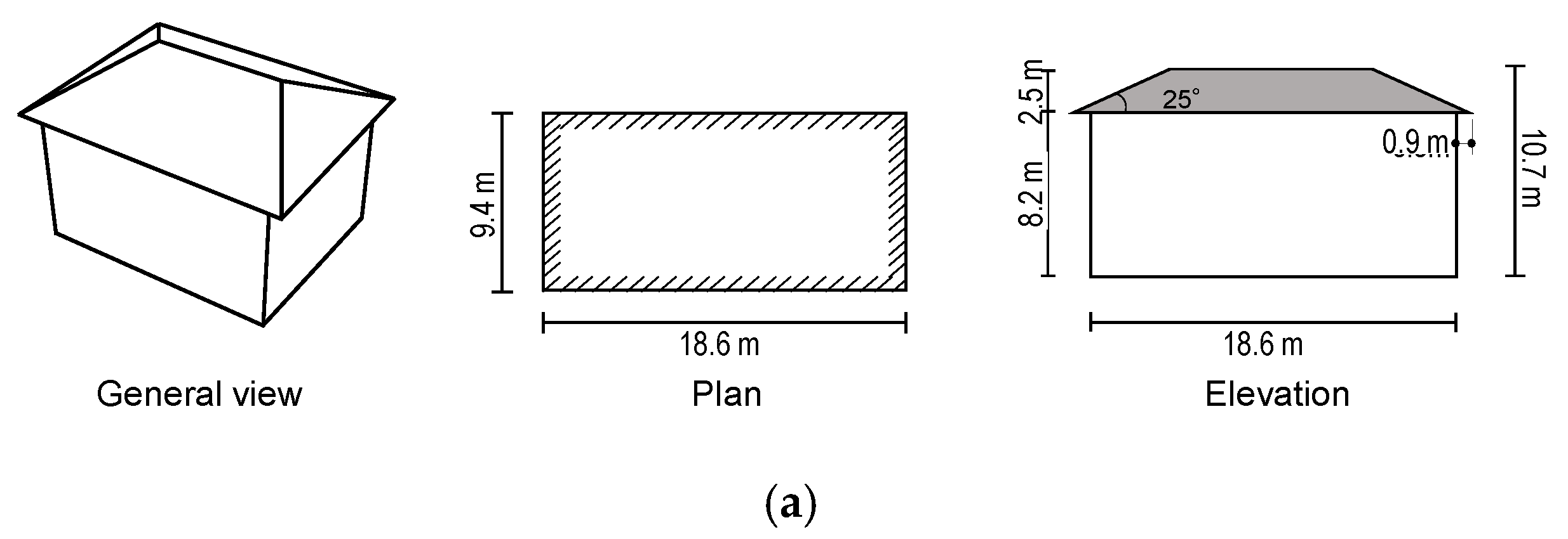
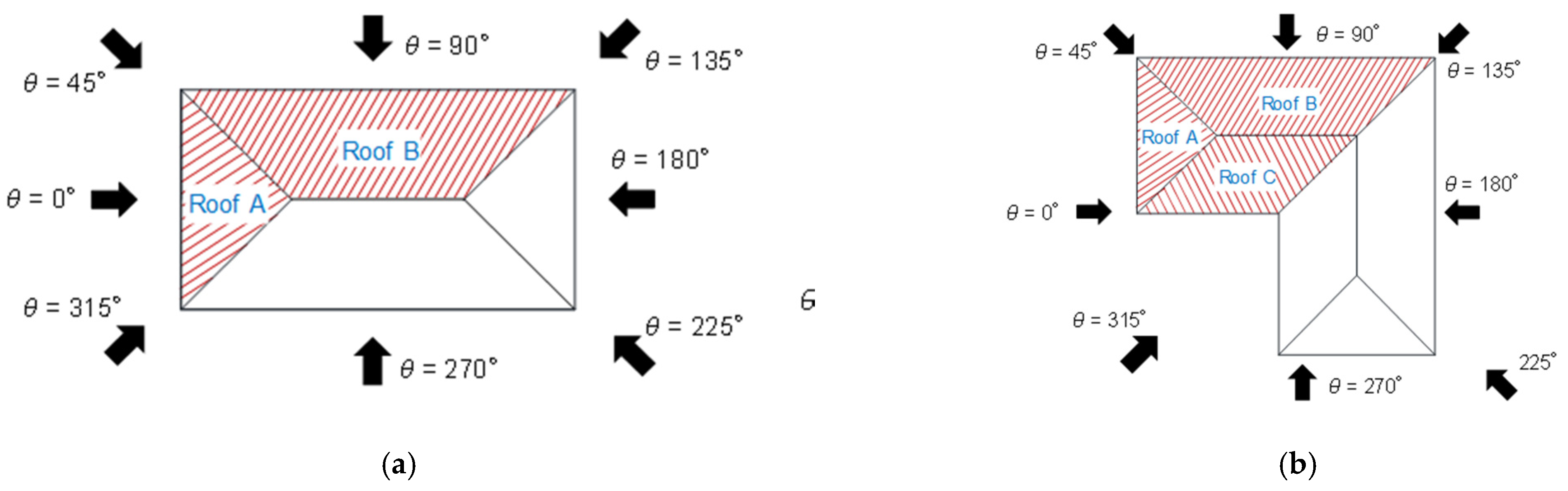
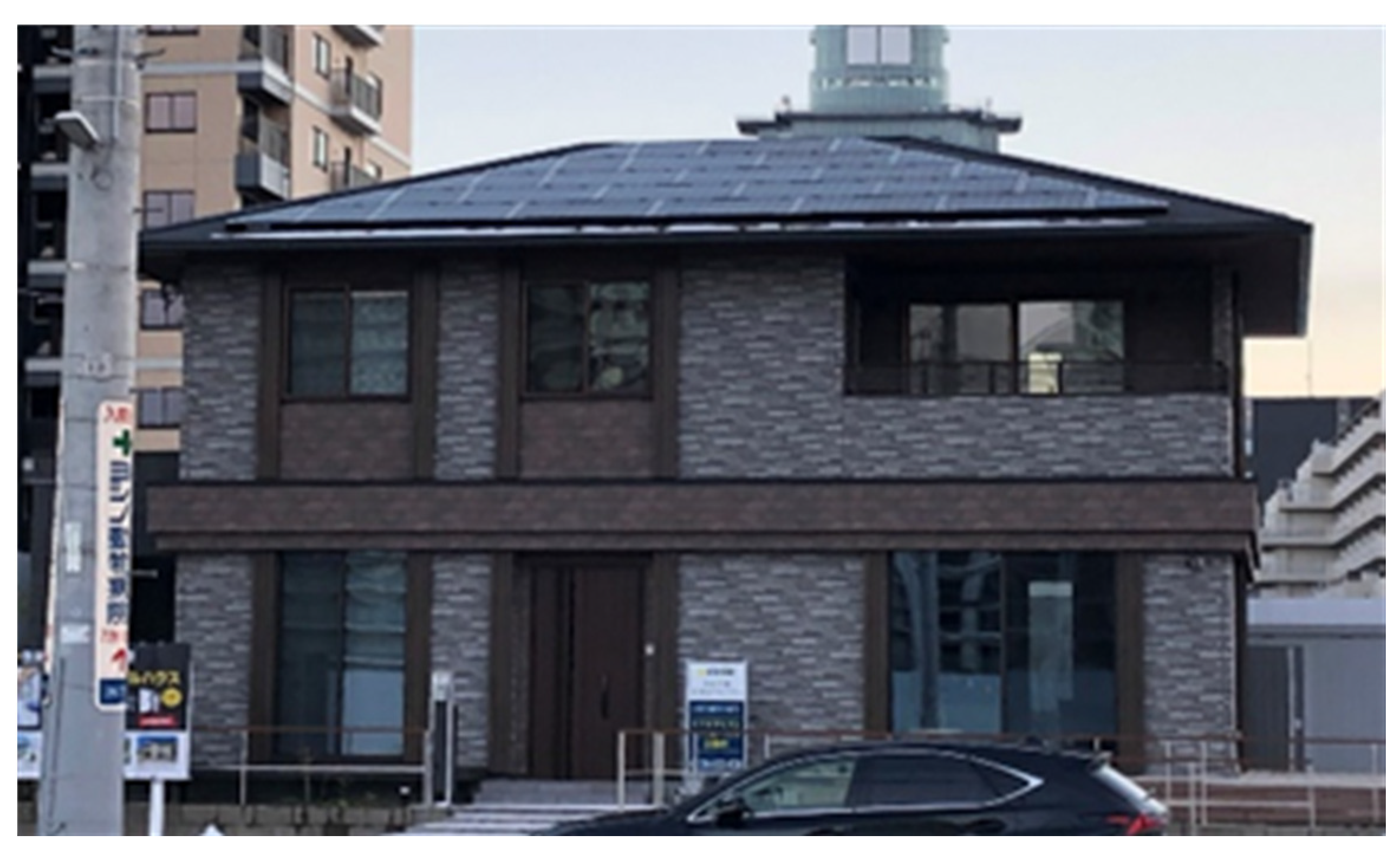
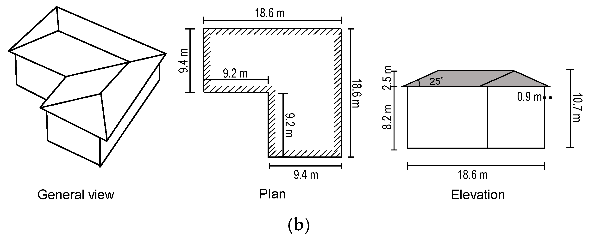
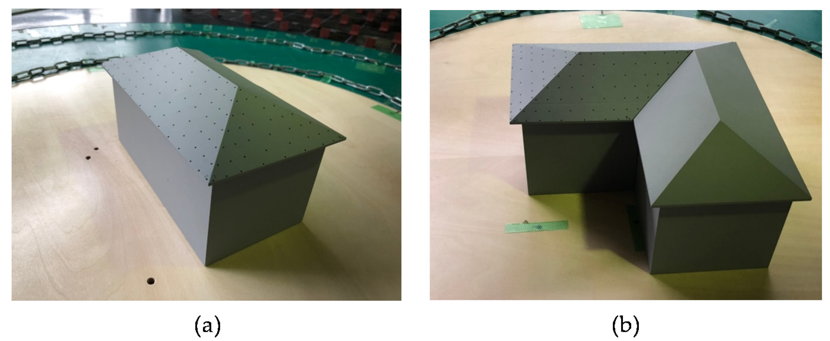
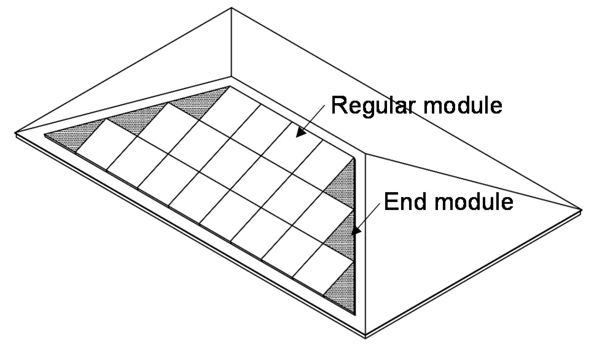
2.1. Investigated Buildings and Wind Tunnel Models

The subject of this study is PV panels mounted on hip roofs of two kinds of two-story residential houses with rectangular and L-shaped plans, as shown in Figure 2, which are called Buildings 1 and 2, respectively. The roof pitch, β, is 25°. The shape and dimensions of these buildings were determined from a survey of current residential houses in Japan; that is, these buildings are typical of current residential houses in Japan. The wind tunnel models were made by using 2 mm thick acrylic plates for the walls and a 3D printer for the roofs. The geometric scale λ_L was 1/100 (see Figure 3). Figure 4 shows the pressure tap arrangements on the roofs. Considering the symmetry of the model, the pressure taps were arranged on Roofs A and B for Building 1 and on Roofs A–C for Building 2. The number of pressure taps was 120 for Building 1 and 176 for Building 2. The diameter of pressure taps was 0.6 mm. The pressure taps were connected to pressure transducers (Wind Engineering Institute, MAPS-02) via flexible vinyl tubes of 1 m length and 1 mm ID.

2.2. Wind Tunnel Flow

Pressure measurements were carried out in an Eiffel-type wind tunnel at the Department of Architecture and Building Science, Tohoku University, which has a working section 1.4 m wide, 1.0 m high and 6.5 m long. The wind tunnel flow is a turbulent boundary layer generated on the wind tunnel floor by using a spire and roughness blocks. The power-law exponent, α, for the mean wind speed profile was about 0.27. The intensity, I_ref, and the integral scale, L_x, of turbulence at a reference height of z_ref = 10 cm (10 m at full scale, which is nearly equal to the height of the rooftop of the buildings) were about 0.17 and 0.2 m, respectively. Comparing these values of α, I_ref and L_x with the specified values in the AIJ Recommendations for Loads on Buildings [24] (referred to as ‘AIJ-RLB’, hereafter) for suburban exposure (Terrain Category III), we found that α is larger, whereas I_ref and L_x were smaller. In particular, the value of L_x was much smaller than the target. The similarity of the wind tunnel flow with natural winds was discussed in our previous paper [23]. Regarding the integral scale of turbulence, the wind tunnel flow satisfied the criteria specified by Tieleman et al. [25,26,27] for wind tunnel flow. It was concluded that the wind tunnel flow was acceptable for the purpose of the present study. The blockage ratio, Br, defined as the ratio of the model’s vertical cross section to the wind tunnel’s cross section (1.4 m $\times$ 1.0 m), was about 2%, at most. The mean wind speed, U_H, at the mean roof height, H (=9.45 cm), was about 8.5 m/s. The Reynolds number, Re, defined in terms of U_H and H, was about 5.4 × 10⁴. The values of Br and Re satisfied the conditions specified by the ASCE Wind Tunnel Testing for Buildings and Other Structures [28], i.e., Br < 5% and Re > 1.1 × 10⁴. The wind direction, θ, defined as shown in Figure 5, was varied at an increment of 5°. The range of θ depends on the roof, considering the symmetry of the building, for example, from 0° to 180° for Roof A of Building 1 and from 0° to 355° for all roofs of Building 2. The pressure coefficient distributions on the whole roof area at various wind directions can be obtained from the measured distributions on the half area of the roof (hatched areas in Figure 5a,b).

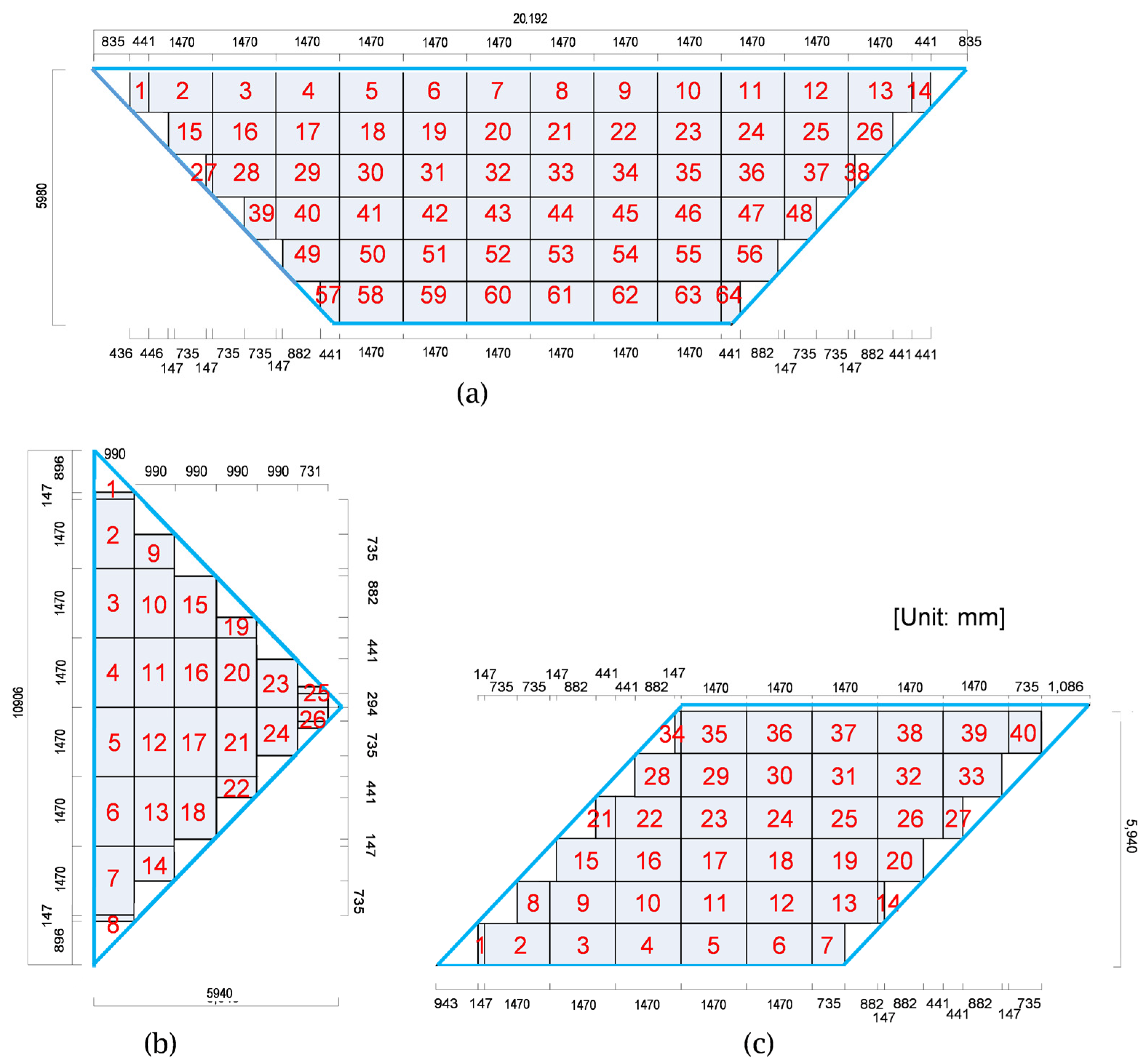
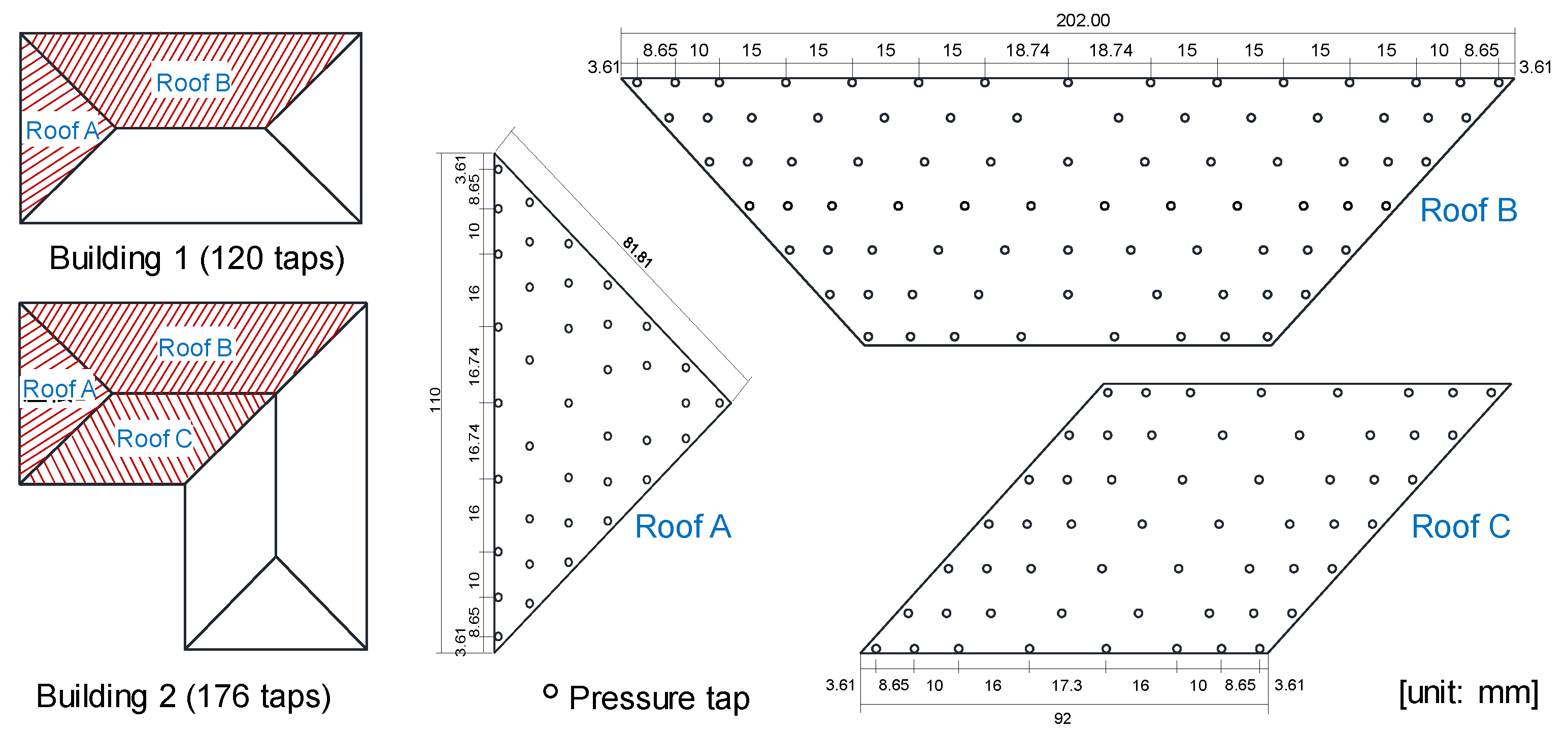
2.3. Wind Pressure Measurement

The design wind speed (10 min mean wind speed), U_H, at the mean roof height, H, was 27.8 m/s, which was determined based on the AIJ-RLB, with an assumption that the ‘basic wind speed’, U₀ was 35 m/s and the terrain category was III. The mean wind speed, U_H, was set to 8.5 m/s in the wind tunnel experiment, as mentioned above. Therefore, the velocity scale, λ_V, of the wind tunnel flow was 1/3.27. Consequently, the time scale, λ_T, was calculated as 1/30.6. The sampling frequency and period of pressure measurements were 800 Hz and 19.6 s (26 Hz and 600 s at full scale), respectively. A low-pass filter with a cut-off frequency of 300 Hz was used to eliminate high-frequency noise included in the output of pressure transducers. The measurements were carried out 10 times.

The wind pressure coefficient, $C_{pe}$, was defined in terms of the velocity pressure, $q_H$ (=$\frac{1}{2}\rho U_H^2$, where ρ is the air density), of the approach flow. The statistical values of $C_{pe}$, such as the maximum and minimum peak pressure coefficients, ${\widehat{C}}_{pe}$ and ${\check{C}}_{pe}$, during 10 min at full scale, were evaluated by applying ensemble averaging to the results of ten measurements. The tubing system used in the pressure measurements caused a distortion of fluctuating pressures, which was compensated in the frequency domain by using the transfer function of the measuring system.

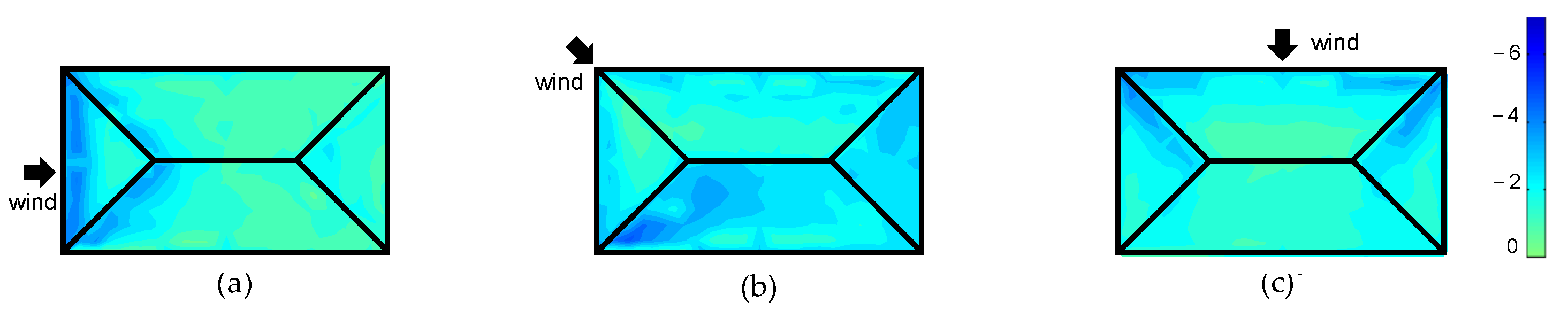
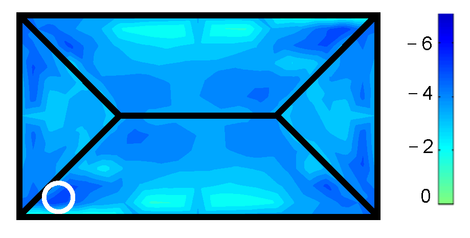
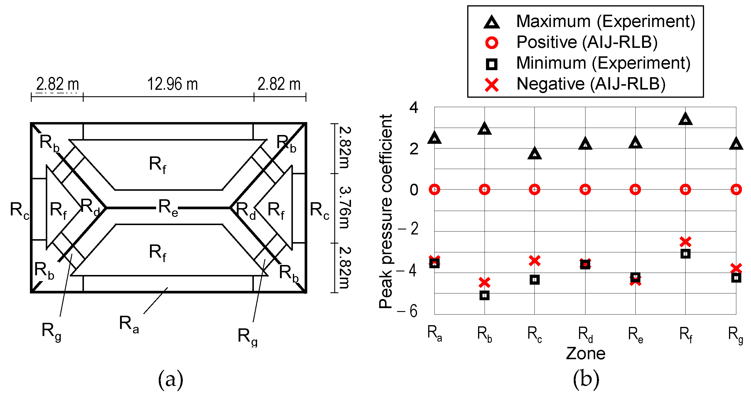
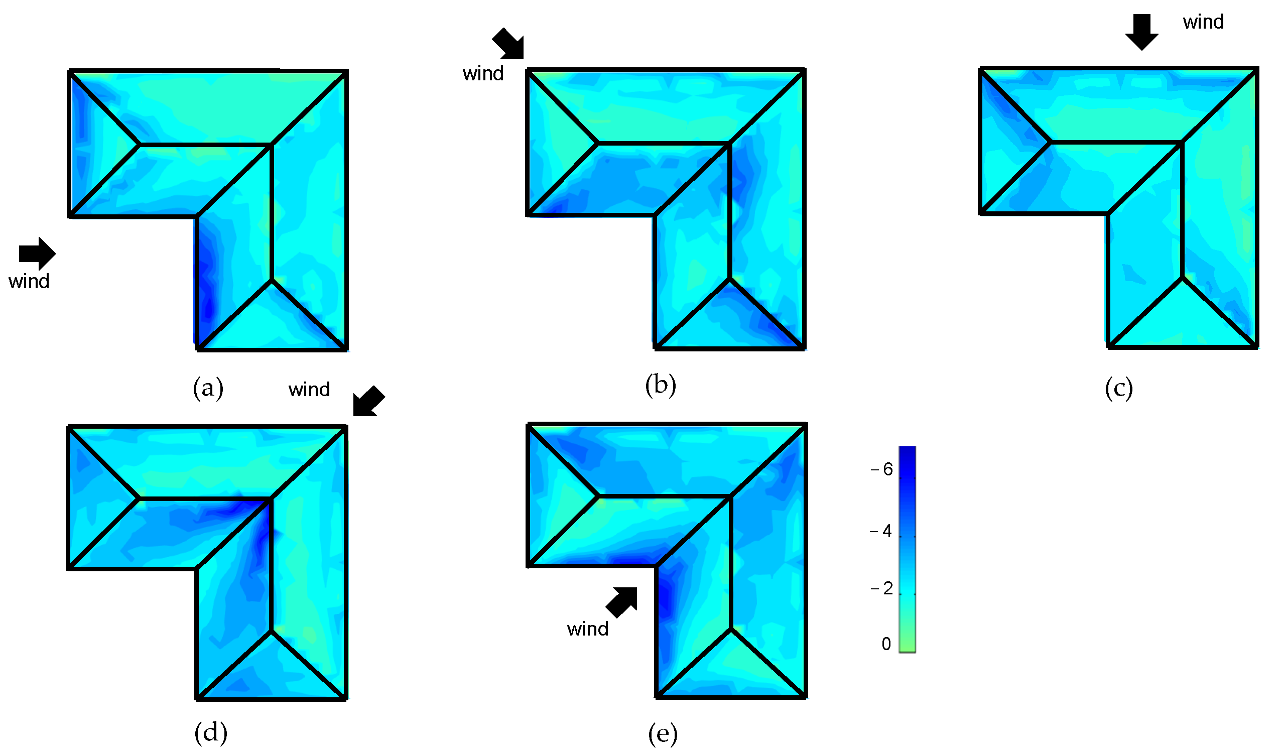
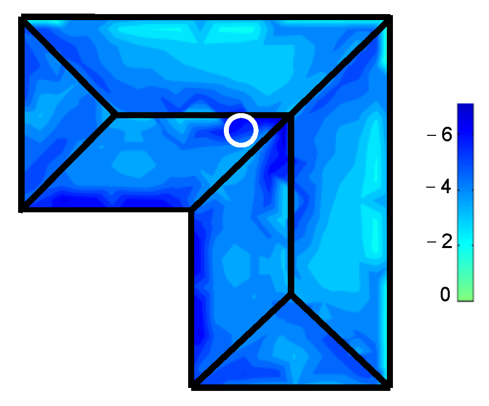
2.4. Wind Pressure Distribution on the Roof

A wind tunnel experiment was carried out to obtain the time histories of wind pressure coefficients on the roof, which were used for the numerical simulation of the layer pressures (Section 3). However, it seems interesting to study the characteristics of wind pressures on the roofs because they significantly affect the wind loads on PV panels. Considering the construction of PV systems, the critical load on the panels is thought to be up-lift force. Therefore, we focused on the negative pressures.

Figure 6 shows the contours of the minimum peak pressure coefficients, ${\check{C}}_{pe}$, on the roof of Building 1 at θ = 0°, 45° and 90°. The values of ${\check{C}}_{pe}$ were derived from the time histories of $C_{pe}$, to which no moving average was applied. In normal winds, e.g., at θ = 0° and 90°, large suctions occur near the windward eaves and corner ridges (declining ridges). On the other hand, in diagonal winds, e.g., at θ = 45°, larger suctions occur near the leeward corner ridge. Figure 7 shows the contours of the most critical minimum peak pressure coefficient, ${\check{C}}_{pe,\mathrm{cr}}$, irrespective of wind direction, i.e., the minimum value of ${\check{C}}_{pe}$ among all wind directions at each pressure tap. The minimum value of ${\check{C}}_{pe,\mathrm{cr}}$ among all pressure taps was −5.08, which occurred at a tap marked by a white circle in Figure 7 when θ = 35°. Note that the ${\check{C}}_{pe,\mathrm{cr}}$ distribution on the roof is not necessarily symmetric with respect to the center lines parallel to the long and short sides. This is due to an avoidable error involved in the experiment. The characteristics of the minimum pressure coefficients on the roofs observed here are consistent with those reported in previous studies [29,30,31,32,33,34,35,36].

The AIJ-RLB specifies positive and negative peak pressure coefficients for designing cladding/components of roofs. The roof is divided into several zones, as shown in Figure 8a, and positive and negative peak pressure coefficients are provided for each zone as a function of the building geometry. The specification is based on the results of wind tunnel experiments [33,34,35]. Figure 8b compares the specified values with the values of ${\widehat{C}}_{pe,\mathrm{cr}}$ and ${\check{C}}_{pe,\mathrm{cr}}$ obtained in our experiment. The AIJ-RLB specifies the positive peak pressure coefficients as zero when θ ≤ 30°. However, the present results show relatively large positive values of up to about 3.3. This implies that the specification should be revised appropriately, although positive pressures are not so important for cladding/components of roofs. By comparison, regarding the negative peak pressure coefficients, the present results correspond well to the specified values. In Zones R_b and R_c, however, the present results are somewhat larger in magnitude than the specified values. The difference may be attributed to the effect of roof’s overhang on the pressures. Note that the AIJ-RLB specification is based on the results for buildings with no overhangs.

Contours of ${\check{C}}_{pe}$ on the whole roof of Building 2 at various wind directions are illustrated in Figure 9. When θ = 0° and 315°, high peak suctions occur in the regions along the eaves near the building re-entrant corner. The magnitude is larger than that along the windward eaves of Building 1 in normal winds. When θ = 135°, high peak suctions occur along the roof valley, which may be induced by conical vortices, judging from the distribution pattern of peak suctions. The minimum value of ${\check{C}}_{pe,\mathrm{cr}}$ among all pressure taps is −6.96, observed at a point marked by a white circle in Figure 10 when θ = 130°. This value is much larger in magnitude than that for Building 1 (see Figure 8). A similar feature was observed by Shao et al. [37].

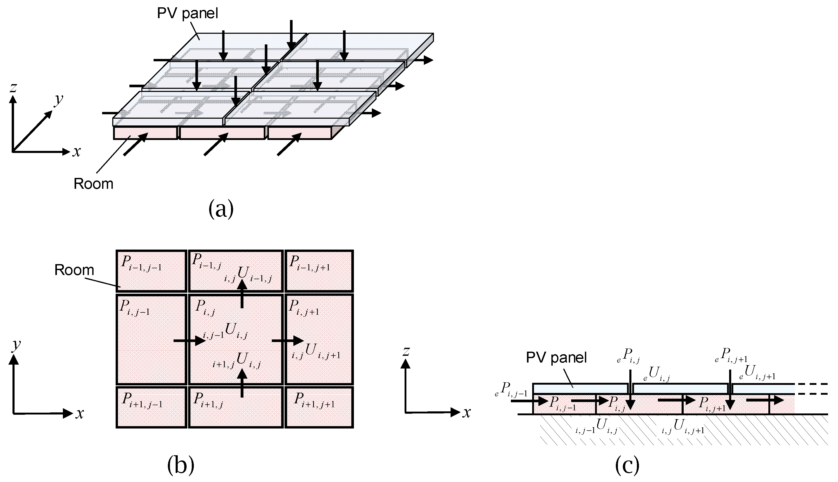
3. Numerical Simulation of Layer Pressures under PV Panels

3.1. Basic Concept and Assumptions

The method of simulation employed here is the same as that we used in our previous studies [22,23]. The application of this method to the evaluation of layer pressures under PV panels was discussed in detail in our previous paper [23]. A comparison between simulation and wind tunnel experiment was made for the mean and peak wind force coefficients of PV panels installed on a simple square-roof building model, and a good agreement was obtained, indicating that the proposed method could be useful for evaluating wind loads on PV panels installed parallel to hip roofs of low-rise buildings. Regarding the details of the simulation method, refer to Uematsu et al. [23]. Only the outline of this method is presented here.

The problem is similar to the multiroom ventilation of a building. The space is divided into many subspaces, as schematically illustrated in Figure 11; the subspace is called ‘room’ in this paper. Note that Figure 11 is the simplest model for showing the basic concept of this simulation method. The x and y axes are parallel to the roof surface, whereas the z axis is normal to the roof surface. P represents the pressure in the room, and U represents the speed of the gap or cavity flow. The subscripts i and j represent the room number in a matrix form, and ‘e’ means outside. The pressure in each room, assumed to be spatially uniform, is a function of time. The gap and cavity flows, which are caused by the pressure difference between adjacent rooms or between the external space and the room, are governed by the unsteady Bernoulli equation. The layer pressure was calculated based on the mass balance of the air flowing into and out of the room, assuming the weak compressibility of the air and an adiabatic condition.

The external pressure coefficients, C_pe, at the gaps were obtained from the above-mentioned wind tunnel experiment. The C_pe value at the center of the gap between two PV panels was used as a representative value for the gap. However, the C_pe values at these points were not directly obtained from the wind tunnel experiment because the location of pressure taps on the wind tunnel model did not coincide with that of these points. Hence, a spatial interpolation using the cubic spline function was employed. Furthermore, because the time step used in the numerical simulation of layer pressures was much smaller than the sampling interval of pressure measurements in the wind tunnel experiment, a temporal interpolation using the cubic spline function was employed. The shape resistance coefficient, C_L, for the cavity flows in the x and y directions and the pressure loss coefficient (shape resistance coefficient), C_Le, for the gap flows in the z direction depend on the cavity and gap configurations. However, they were assumed to be 1.0 for simplicity [23]. This assumption should be validated by a test with full-scale specimens of cavity and gap, as was done in our previous study [38]. This is a subject left for our future study.

3.2. Practical Application

Figure 12 shows the arrangements and numbering of PV panels mounted on Roofs A–C. The PV panel was 1.47 m long and 0.99 m wide. Some small rectangular panels were placed near the corner ridges. The gap width, G, between PV panels along the short edges was set to 5 mm as a default, except in Section 3.3, where the effects of G on the wind loads of PV panels and roofing are discussed. The PV panels were arranged with no gaps along the long edges. When the gap along the short sides was introduced, the length of the long side of PV panels was assumed to be shortened by G. This assumption made the analysis easier. The thickness, t_panel, and the clearance, H_panel, were 30 mm and 70 mm, respectively. The space under the PV panels was divided into many small rooms of 990 mm × 294 mm in plane, as shown in Figure 13, which made it possible to evaluate the spatial variation of layer pressure in the PV panels’ long-side direction.

The net wind force per unit area on a PV panel is given by the difference between pressures on the top and bottom surfaces. The top-surface pressure can be replaced by the external pressure acting on the bare roof because the thickness, t_panel, is small. The bottom-surface pressure is equal to the layer pressure obtained from the numerical simulation. Therefore, the wind force coefficient (pressure difference coefficient) C_f of the PV panel may be given by the following equation:

$$C_f=C_{pe}-C_{pl}$$

(1)

where C_pl represents ‘layer pressure coefficient’ defined in terms of q_H. The net wind force, F, on a PV panel, called ‘panel force’ in this paper, is calculated by integrating the pressure difference over the panel area. F is normalized by q_H and the area of the panel (A_panel) to yield the panel force coefficient C_f,panel.

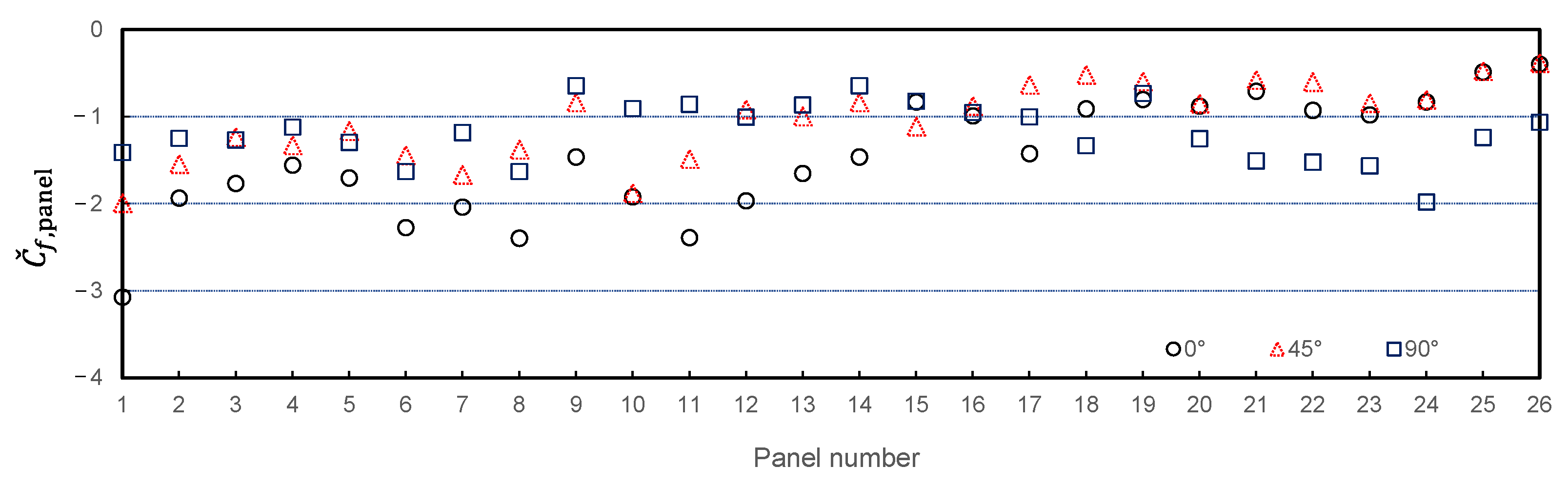
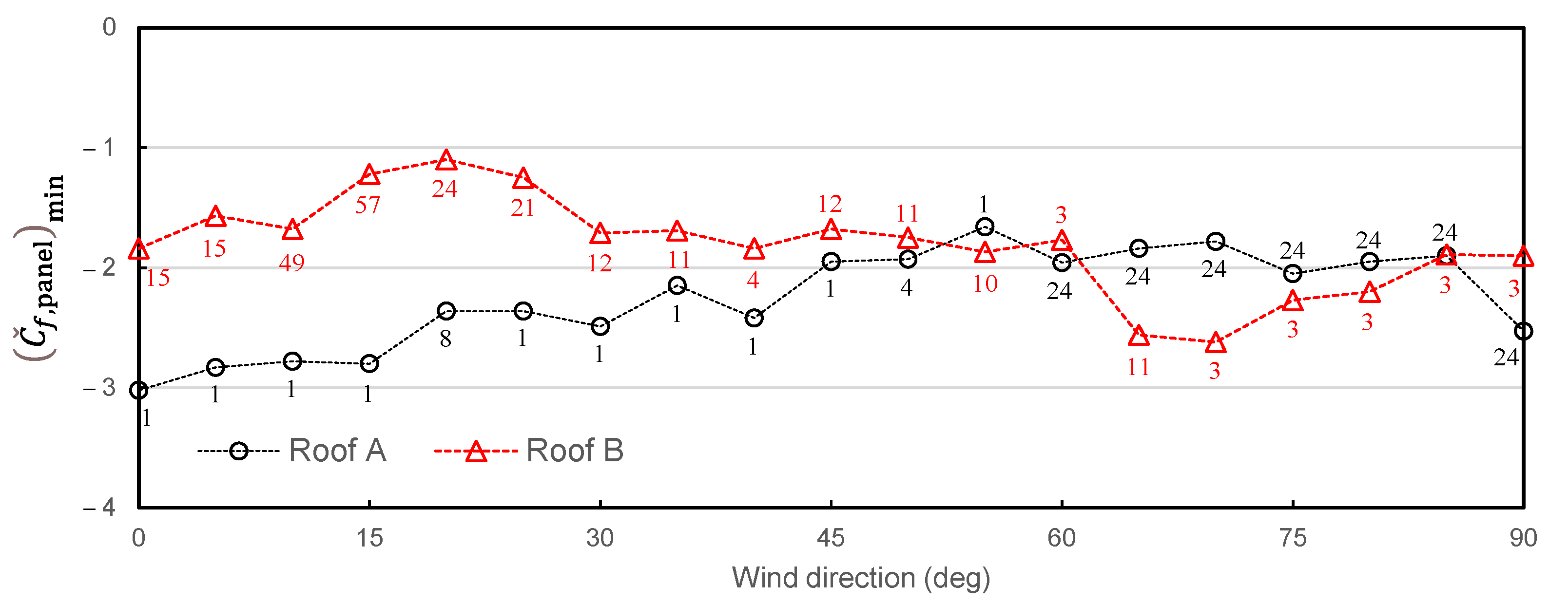
3.3. Wind Force Ccoeffcients of PV Panels

Figure 14 shows the minimum peak values of $C_{f,\mathrm{panel}}$, represented by ${\check{C}}_{f,\mathrm{panel}}$, among all panels mounted on Roof A of Building 1 when θ = 0°, 45° and 90°. The largest value of $\left|{\check{C}}_{f,\mathrm{panel}}\right|$ occurred on Panel 1 when θ = 0°. However, because the area of this panel was so small, the net wind force was not very large. Except for this panel, the values of $\left|{\check{C}}_{f,\mathrm{panel}}\right|$ were all smaller than 2.5. Then, the minimum value of ${\check{C}}_{f,\mathrm{panel}}$ among all panels on each roof (A, B or C) at each wind direction was obtained. Figure 15 and Figure 16 show the results for Buildings 1 and 2, respectively, in which the figure near each marker represents the panel number providing the largest $\left|{\check{C}}_{f,\mathrm{panel}}\right|$ value among all panels. It is clear that larger up-lift forces were induced on the panels located along the eaves and ridges. In the case of Building 2, larger up-lift forces were induced on the panels placed near the top of the roof valley. Such large values of $\left|{\check{C}}_{f,\mathrm{panel}}\right|$ may be due to large suctions generated by the flow separation at the eaves and ridges (see Figure 9 and Figure 10). The $\left|{\check{C}}_{f,\mathrm{panel}}\right|$ values for Building 2 were generally larger than those for Building 1. These features are consistent with the distributions of ${\check{C}}_{pe}$, as shown in Figure 6 and Figure 9.

In Japan, the design of PV systems is generally based on JIS C 8955 [1], as mentioned above. This standard provides positive and negative wind force coefficients, C_a, of PV panels mounted parallel to sloped roofs as a function of roof pitch, β (deg). The negative wind force coefficients for regular rectangular modules (panels) and triangular end modules on a hip roof (see Figure 17) are specified as follows:

$$C_a=-1.5+0.015\beta$$

(2)

for regular rectangular modules and

$$C_a=-2.3+0.033\beta$$

(3)

for triangular end modules.

When β = 25°, the value of $C_a$ is calculated as −1.125 for regular modules and −1.475 for end modules. The dynamic load effect of fluctuating wind pressures is considered by ‘gust effect factor’, G_f. The value of G_f depends on the terrain of the construction site. For terrain category III (suburban exposure), G_f is specified as 2.5. As mentioned above, the wind force coefficients are not specified for PV panels placed in the edge zones up to 0.3 m from the roof edges because such panels may be subjected to large up-lift forces, and therefore, installing PV panels in the edge zones is not recommended. In a strict sense, we cannot make a direct comparison between the present results for PV panels installed along the edges and the specified values in JIS C 8955. However, it seems interesting to compare these two values with each other. The minimum peak panel force coefficient, ${\check{C}}_{f,\mathrm{panel}}$, obtained in this study should be compared with the product of $C_a$ and $G_f$, which is −2.8 for regular modules and −3.7 for end modules. The values of ${\check{C}}_{f,\mathrm{panel}}$ for small panels, such as Panel 1 on Roof A, can be compared with −3.7 for the end modules, whereas those for the other panels can be compared with −2.8 for the regular modules. Figure 15 and Figure 16 indicate that the values of ${\check{C}}_{f,\mathrm{panel}}$ are generally smaller in magnitude than the specified values in JIS C 8955 [1].

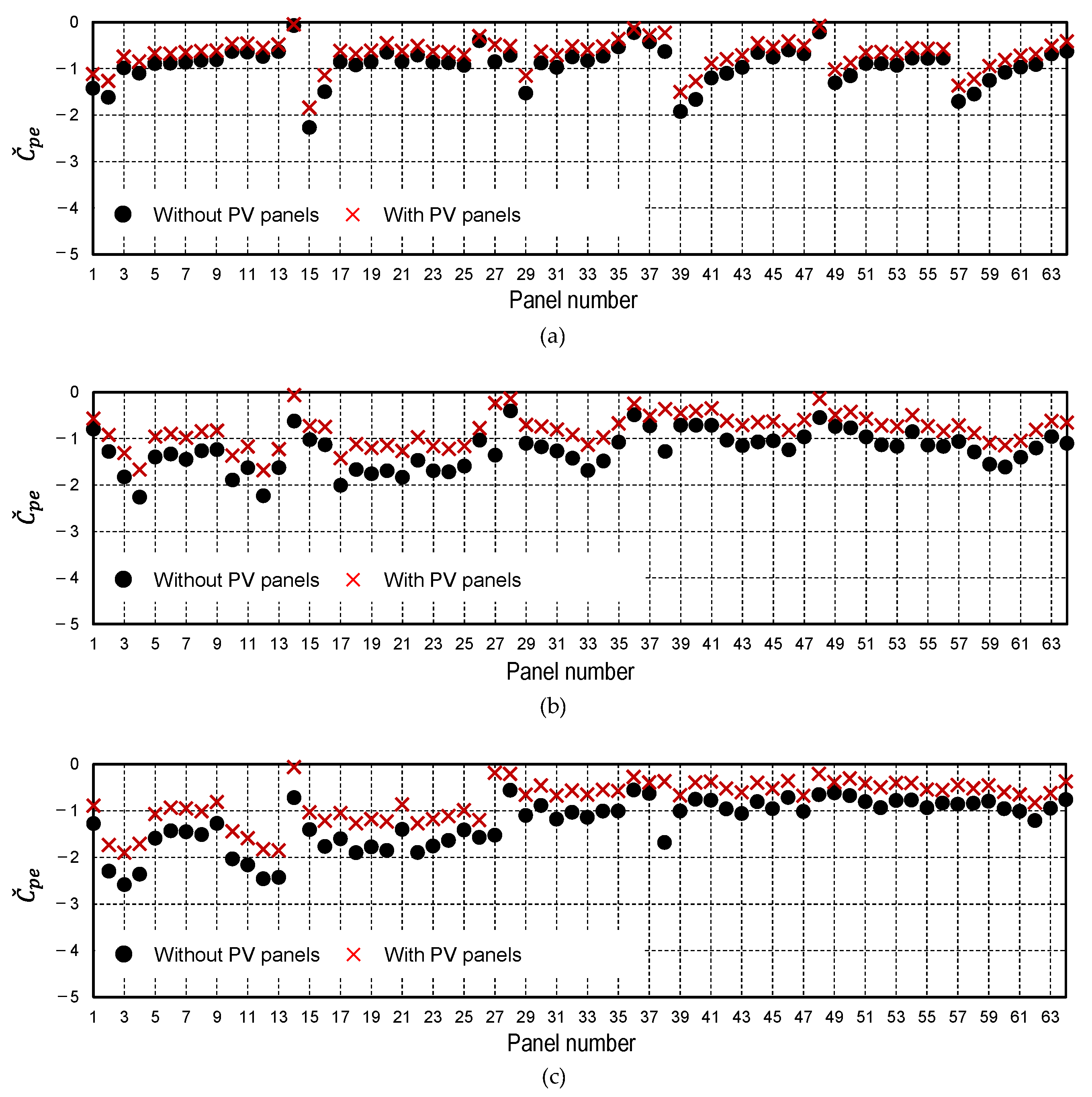
3.4. Wind Pressure Coeffcients on the Roof

Figure 18 and Figure 19 show how the pressures on the roof are affected by installing PV panels on the roof when θ = 0°, 45° and 90°, in which case the minimum peak pressure coefficients, ${\check{C}}_{pe}$, at the panels’ centers on the roof are compared with those on the bare roof. It is clear that the magnitude of ${\check{C}}_{pe}$ near the roof edges decreases significantly when PV panels are installed on the roof, particularly in the edge zones, where large peak suctions are induced. This result implies that PV panels can be used as a device for reducing wind pressures on the roofing or for improving the wind-resistance performance of roofing [22,23].

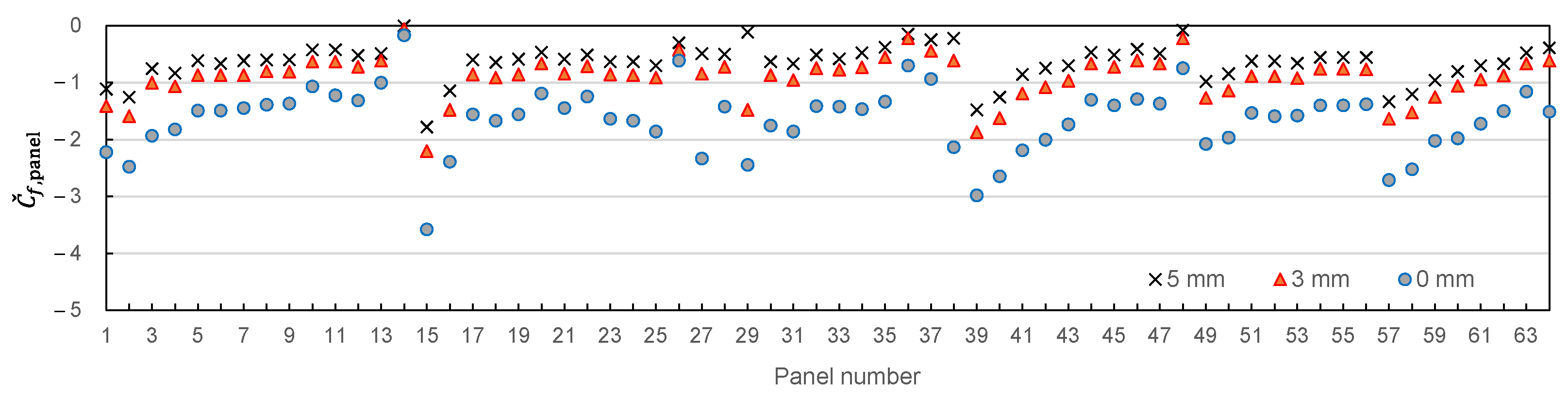
3.5. Effect of Gap Width on the Wind Loads on PV Panels

Figure 20 and Figure 21 show the effect of gap width, G, on the minimum peak panel force coefficients, ${\check{C}}_{f,\mathrm{panel}}$, on Roof B of Buildings 1 and 2, respectively, when θ = 90°, in which case G was varied from 0 to 5 mm. At this wind direction, larger up-lift forces are generated on the PV panels placed near the windward eaves. It was found that the values of $\left|{\check{C}}_{f,\mathrm{panel}}\right|$ generally decreased with an increase in G. The results for G = 10 mm (not shown here) were found to be almost the same as those for G = 5 mm. Therefore, it can be concluded that G = 5 mm is the optimum gap width from the viewpoint of wind load reduction within the limits of the present analysis. The values of ${\check{C}}_{f,\mathrm{panel}}$ for G = 0 mm are larger in magnitude than the specified values in JIS C 8955 for several panels near the roof edges. That is, the specification cannot be applied to PV panels installed near roof edges when G = 0 mm. However, when PV panels are installed with gaps along the short sides, the values of ${\check{C}}_{f,\mathrm{panel}}$ become smaller in magnitude than the specified values.

4. Concluding Remarks

Wind loads on PV panels mounted on hip roofs of low-rise buildings were investigated numerically. Our focus was on the up-lift (negative) wind forces. The roof pitch, β, was fixed to 25° as a representative value for residential houses in Japan. Two types of plans, i.e., rectangular and L-shaped plans, were tested. Because of the low thickness values of PV panels, together with a small clearance, H_panel, between PV panels and roof, it is difficult to make wind tunnel models of PV panels with the same geometric scale as that for buildings. Hence, we focused on a numerical simulation using the unsteady Bernoulli equation to estimate the layer pressures between PV panels and the roof. The simulation used the time histories of wind pressure coefficients on the roof without PV panels (bare roof), which had been obtained in a turbulent boundary layer. Furthermore, we proposed installing PV panels with small gaps between them along the short sides. It was expected that the gaps might produce pressure equalization, resulting in a significant reduction in the net wind forces on PV panels.

First, the wind pressure distributions on the bare roof were measured in a turbulent boundary layer. It was found that large peak suctions occurred near the roof edges (eaves and ridges) due to flow separations at the edges. The peak suctions were larger in magnitude for the L-shaped building than for the rectangular building. The observed characteristics of wind pressure distributions were consistent with previous experimental results.

Then, numerical simulations were carried out to estimate the layer pressures under PV panels. The simulation results were combined with the experimental results of external pressures on the roof to calculate the wind forces on PV panels. The gap width, G, between PV panels along the short sides was tentatively set to 5 mm. The results indicated that large up-lift forces were induced on PV panels near the roof edges. Furthermore, the minimum peak panel force coefficients, ${\check{C}}_{f,\mathrm{panel}}$, for the L-shaped building were larger in magnitude than those for the rectangular building. The values of ${\check{C}}_{f,\mathrm{panel}}$ were almost consistent with the specified values in JIS C 8955, although the standard does not specify the wind force coefficients for PV panels installed in edge zones. The PV panels also significantly reduced the magnitude of external wind pressures acting on the roof.

Finally, the effect of gap width, G, on the wind forces on PV panels was investigated. The value of G was varied from 0 to 10 mm. When G = 0 mm, the values of ${\check{C}}_{f,\mathrm{panel}}$ for some panels were larger in magnitude than the specified values in JIS C 8955. With an increase in G, the magnitude of ${\check{C}}_{f,\mathrm{panel}}$ generally decreased. The results for G = 10 mm were almost the same as those for G = 5 mm. Therefore, it may be concluded that the optimum value of G is 5 mm within the limits of the present analysis.

Further analyses for other roof pitches and building shapes are required before these results can be generalized.

References

1. JIS C 8955:2017; Japanese Industrial Standard. Load Design Guide on Structures for Photovoltaic Array. Japanese Standards Association: Tokyo, Japan, 2017.
2. Wood, G.S.; Denoon, R.; Kwok, K.C.S. Wind loads on industrial solar panel arrays and supporting roof structure. Wind. Struct. 2001, 4, 481–494. [Google Scholar] [CrossRef]
3. Kopp, G.A.; Farquhar, S.; Morrison, M.J. Aerodynamic mechanisms for wind loads on tilted, roof-mounted, solar arrays. J. Wind Eng. Ind. Aerodyn. 2012, 111, 40–52. [Google Scholar] [CrossRef]
4. Kopp, G.A.; Banks, D. Use of the wind tunnel test method for obtaining design wind loads on roof-mounted solar arrays. J. Struct. Eng. 2013, 139, 284–287. [Google Scholar] [CrossRef]
5. Banks, D. The role of corner vortices in dictating peak wind loads on tilted flat solar panels mounted on large, flat roofs. J. Wind. Eng. Ind. Aerodyn. 2013, 123, 192–201. [Google Scholar] [CrossRef]
6. Browne, M.T.L.; Gibbons, M.P.M.; Gamble, S.; Galsworthy, J. Wind loading on tilted roof-top solar arrays: The parapet effect. J. Wind. Eng. Ind. Aerodyn. 2013, 123, 202–213. [Google Scholar] [CrossRef]
7. Cao, J.; Yoshida, A.; Saha, P.K.; Tamura, Y. Wind loading characteristics of solar arrays mounted on flat roofs. J. Wind. Eng. Ind. Aerodyn. 2013, 123, 214–225. [Google Scholar] [CrossRef]
8. Kopp, G.A. Wind loads on low-profile, tilted, solar arrays placed on large, flat, low-rise building roofs. J. Struct. Eng. 2014, 140, 04013057. [Google Scholar] [CrossRef]
9. Stathopoulos, T.; Zisis, I.; Xypnitou, E. Local and overall wind pressure and force coefficients for solar panels. J. Wind. Eng. Ind. Aerodyn. 2014, 125, 195–206. [Google Scholar] [CrossRef]
10. Wang, J.; Yang, Q.; Tamura, Y. Effects of building parameters on wind loads on flat-roof-mounted solar arrays. J. Wind. Eng. Ind. Aerodyn. 2018, 174, 210–224. [Google Scholar] [CrossRef]
11. Wang, J.; Phuc, P.V.; Yang, Q.; Tamura, Y. LES study of wind pressure and flow characteristics of flat-roof-mounted solar arrays. J. Wind. Eng. Ind. Aerodyn. 2020, 198, 104096. [Google Scholar] [CrossRef]
12. Wang, J.; Yang, Q.; Phuc, P.V.; Tamura, Y. Characteristics of conical vortices and their effects on wind pressures on flat-roof-mounted solar arrays by LES. J. Wind. Eng. Ind. Aerodyn. 2020, 200, 104146. [Google Scholar] [CrossRef]
13. Alrawashdeh, H.; Stathopoulos, T. Wind loads on solar panels mounted on flat roofs: Effect of geometric scale. J. Wind. Eng. Ind. Aerodyn. 2020, 206, 104339. [Google Scholar] [CrossRef]
14. Geurts, C.; Blackmore, P. Wind loads on stand-off photovoltaic systems on pitched roof. J. Wind. Eng. Ind. Aerodyn. 2013, 123, 239–249. [Google Scholar] [CrossRef]
15. Aly, A.M.; Bitsuamlak, G.T. Wind-induced pressures on solar panels mounted on residential homes. J. Archit. Eng. 2014, 20, 04013003. [Google Scholar] [CrossRef]
16. Stenabaugh, S.E.; Iida, Y.; Kopp, G.A.; Karava, P. Wind loads on photovoltaic arrays mounted parallel to sloped roofs on low-rise buildings. J. Wind. Eng. Ind. Aerodyn. 2015, 139, 16–26. [Google Scholar] [CrossRef]
17. Leitch, C.J.; Ginger, J.D.; Holmes, D.J. Wind loads on solar panels mounted parallel to pitched roofs, and acting on the underlying roof. Wind. Struct. 2016, 22, 307–328. [Google Scholar] [CrossRef]
18. Naeiji, A.; Raji, F.; Zisis, I. Wind loads on residential scale rooftop photovoltaic panels. J. Wind. Eng. Ind. Aerodyn. 2017, 168, 228–246. [Google Scholar] [CrossRef]
19. Takamori, K.; Nakagawa, N.; Yamamoto, M.; Okuda, Y.; Taniguchi, T.; Nakamura, O. Study on design wind force coefficients for photovoltaic modules installed on low-rise building. AIJ J. Technol. Des. 2015, 21, 67–70. (In Japanese) [Google Scholar] [CrossRef] [Green Version]
20. Agarwall, A.; Irtaza, H.; Shahab, K. 2020, Aerodynamic wind pressure on solar PV arrays mounted on industrial pitched roof building. In Proceedings of the International Conference on Recent Advances in Engineering & Science (ICRAES-2020), Aligarh, India, 4–6 September 2020. [Google Scholar]
21. Li, J.; Tong, L.; Wu, J.; Pan, Y. Numerical investigation of wind influences on photovoltaic arrays mounted on roof. Eng. Appl. Comput. Fluid Mech. 2019, 13, 905–922. [Google Scholar] [CrossRef] [Green Version]
22. Uematsu, Y.; Yambe, T.; Watanabe, T.; Ikeda, H. The Benefit of horizontal photovoltaic panels in reducing wind loads on a membrane roofing system on a flat roof. Wind 2021, 1, 44–62. [Google Scholar] [CrossRef]
23. Uematsu, Y.; Yambe, T.; Yamamoto, A. Application of a numerical simulation to the estimation of wind loads on photovoltaic panels installed parallel to hip roofs of residential houses. Wind 2022, 2, 129–149. [Google Scholar] [CrossRef]
24. Architectural Institute of Japan. Recommendations for Loads on Buildings; Architectural Institute of Japan: Tokyo, Japan, 2015. [Google Scholar]
25. Tieleman, H.W.; Reinhold, T.A.; Marshall, R.D. On the wind-tunnel simulation of the atmospheric surface layer for the study of wind loads on low-rise buildings. J. Wind. Eng. Ind. Aerodyn. 1978, 3, 21–38. [Google Scholar] [CrossRef]
26. Tieleman, H.W. Pressures on surface-mounted prisms: The effects of incident turbulence. J. Wind. Eng. Ind. Aerodyn. 1993, 49, 289–299. [Google Scholar] [CrossRef]
27. Tieleman, H.W.; Hajj, M.R.; Reinhold, T.A. Wind tunnel simulation requirements to assess wind loads on low-rise buildings. J. Wind. Eng. Ind. Aerodyn. 1998, 74–76, 675–686. [Google Scholar] [CrossRef]
28. ASCE/SEI 49-12; Wind Tunnel Testing for Buildings and Other Structures. American Society of Civil Engineers: Reston, VA, USA, 2012.
29. Meecham, D.; Surry, D.; Davenport, A.G. The magnitude and distribution of wind-induced pressures on hip and gable roofs. J. Wind. Eng. Ind. Aerodyn. 1991, 38, 257–272. [Google Scholar] [CrossRef]
30. Xu, Y.L.; Reardon, G.F. Variation of wind pressure on hip roofs with roof pitch. J. Wind. Eng. Ind. Aerodyn. 1998, 73, 267–284. [Google Scholar] [CrossRef]
31. Ahmad, S.; Kumar, K. Effect of geometry on wind pressures on low-rise hip roof buildings. J. Wind. Eng. Ind. Aerodyn. 2002, 90, 755–779. [Google Scholar] [CrossRef]
32. Ahmad, S.; Kumar, K. Wind pressures on low-rise hip roof buildings. Wind Struct. 2002, 5, 493–514. [Google Scholar] [CrossRef]
33. Takamori, K.; Nishimura, H.; Asami, R.; Somekawa, D.; Aihara, T. Wind pressures on hip roofs of a low-rise building—Case of square plan. In Proceedings of the National Symposium on Wind Engineering, Tokyo, Japan, 3–5 December 2008; pp. 409–414. (In Japanese). [Google Scholar]
34. Aihara, T.; Asami, Y.; Nishimura, H.; Takamori, K.; Asami, R.; Somekawa, D. An area correct factor for the wind pressure coefficient for cladding of hip roof—The case of square plan hip roof with roof pitch of 20 degrees. In Proceedings of the National Symposium on Wind Engineering, Tokyo, Japan, 3–5 December 2008; pp. 463–466. (In Japanese). [Google Scholar]
35. Terazaki, H.; Katsumura, A.; Uematsu, Y.; Ohtake, K.; Okuda, Y.; Kikuchi, H.; Noda, H.; Masuyama, Y.; Yamamoto, M.; Yoshida, A. Wind force coefficient and gust loading factor for roof and eave. Wind Eng. 2011, 36, 343–361. (In Japanese) [Google Scholar]
36. Shao, S.; Tian, Y.; Yang, Q.; Stathopoulos, T. Wind-induced cladding and structural loads on low-rise buildings with 4:12-splped hip roofs. J. Wind. Eng. Ind. Aerodyn. 2019, 193, 103948. [Google Scholar] [CrossRef]
37. Shao, S.; Stathopoulos, T.; Yang, Q.; Tian, Y. Wind pressures on 4:12-sloped hip roofs of L- and T-shaped low-rise buildings. J. Struct. Eng. 2018, 144, 04018088. [Google Scholar] [CrossRef]
38. Yambe, T.; Uematsu, Y.; Sato, K. Wind Loads on Roofing System and Photovoltaic System Installed Parallel to Flat Roof. In STR-39. In Proceedings of the International Structural Engineering and Construction Holistic Overview of Structural Design and Construction, Limassol, Cyprus, 3–8 August 2020; Vacanas, Y., Danezis, C., Singh, A., Yazdani, S., Eds.; ISEC Press: Fargo, ND, USA, 2020. [Google Scholar]
Figure 1. Hip-roof residential house equipped with a PV system.
Wind 02 00016 g001
Figure 2. Buildings considered in the present paper: (a) Building 1; (b) Building 2.
Wind 02 00016 g002aWind 02 00016 g002b
Figure 3. Wind tunnel models: (a) Building 1; (b) Building 2.
Wind 02 00016 g003
Figure 4. Arrangement of pressure taps on Roofs A–C.
Wind 02 00016 g004
Figure 5. Definition of wind direction, θ: (a) Building 1; (b) Building 2.
Wind 02 00016 g005
Figure 6. Contours of the minimum peak pressure coefficients, C ˇ p e , on the roof of Building 1: (a) θ = 0°; (b) θ = 45°; (c) θ = 90°.
Wind 02 00016 g006
Figure 7. Contours of the most critical minimum peak pressure coefficients, C ˇ p e , cr , irrespective of wind direction, on the roof of Building 1.
Wind 02 00016 g007
Figure 8. Comparison of the experimental values of C ^ p e , cr and C ˇ p e , cr with the positive and negative peak pressure coefficients specified in the AIJ-RLB: (a) Definition of zones; (b) Peak pressure coefficients compared with the specifications.
Wind 02 00016 g008
Figure 9. Contours of the minimum peak pressure coefficients, C ˇ p e , on the roof of Building 2: (a) θ = 0°; (b) θ = 45°; (c) θ = 90°; (d) θ = 135°; (e) θ = 315°.
Wind 02 00016 g009
Figure 10. Contours of the most critical minimum peak pressure coefficients, C ˇ p e , cr , irrespective of wind direction, on the roof of Building 2.
Wind 02 00016 g010
Figure 11. Model of the space under PV panels (conceptual illustration): (a) perspective; (b) xy plane; (c) xz plane.
Wind 02 00016 g011
Figure 12. Arrangement and numbering of PV panels in rooms A–C: (a) Roof A; (b) Roof B; (c) Roof C.
Wind 02 00016 g012
Figure 13. Division of the space under PV panels into ‘rooms’: (a) Roof A; (b) Roof B; (c) Roof C.
Wind 02 00016 g013
Figure 14. Minimum peak panel force coefficients, C ˇ f , panel , on Roof A of Building 1 at θ = 0°, 45° and 90°.
Wind 02 00016 g014
Figure 15. The minimum value of C ˇ f , panel among all panels on each roof of Building 1.
Wind 02 00016 g015
Figure 16. The minimum value of C ˇ f , panel among all panels on each roof of Building 2.
Wind 02 00016 g016
Figure 17. PV panels installed on a hip roof as defined in JIS C 8955 [1].
Wind 02 00016 g017
Figure 18. Minimum peak pressure coefficients, C ˇ p e , on Roof A of Building 1 at the panels’ centers: (a) θ = 0°; (b) θ = 45°; (c) θ = 90°.
Wind 02 00016 g018
Figure 19. Minimum peak pressure coefficients, C ˇ p e , on Roof B of Building 1 at the panels’ centers: (a) θ = 0°; (b) θ = 45°; (c) θ = 90°.
Wind 02 00016 g019
Figure 20. Effect of gap width, G, on the minimum peak panel force coefficients, C ˇ f , panel , on Roof B of Building 1 at θ = 90°.
Wind 02 00016 g020
Figure 21. Effect of gap width, G, on the minimum peak panel force coefficients, C ˇ f , panel , on Roof B of Building 2 at θ = 90°.
Wind 02 00016 g021
Publisher’s Note: MDPI stays neutral with regard to jurisdictional claims in published maps and institutional affiliations.