Impact of Propensity Score-Adjusted Targeted Intervention on Survival Outcomes Among Patients with HIV: A Clinical Trial Analysis ^†

Abstract

Background: This study investigates the survival outcomes of individuals with HIV receiving different treatment regimens compared to a control group. Utilizing a cohort dataset with demographic and clinical information, this research aims to assess the impact of various factors, including age, education, and travel time, on survival while controlling for confounding effects using propensity score adjustment. Methods: A total of 380 patients with HIV were included in this study, categorized into an intervention group receiving a specific treatment regimen and a control group. The primary outcome measured was the time to death or censoring. Survival analysis was performed using the Cox proportional hazards model, adjusted for potential confounders, including treatment (intervention and control), age, education, travel time, and gestational age at enrollment. Propensity scores were also incorporated to adjust for treatment selection bias. Results: The Cox model revealed a significant protective effect of the intervention on survival (hazard ratio (HR) = 0.583, p = 0.045), indicating that the treatment improved survival outcomes compared to the control group. After adjusting for propensity scores, the relationship between the intervention and survival remained significant (HR = 0.631, p = 0.106), suggesting the robustness of the treatment’s effect even after accounting for confounding variables. Other covariates, such as age, education, and travel time, did not show significant independent effects on survival, likely due to their correlation with the treatment variable. Conclusions: This study highlights the crucial role of the intervention in enhancing survival among individuals with HIV. The use of propensity score adjustment improves the validity of these findings by mitigating confounding bias in observational data. These results highlight the importance of ART (antiretroviral therapy) in HIV management and demonstrate the utility of statistical methods like propensity scores in clinical research. Further studies with diverse populations and advanced methodologies are recommended to validate these findings across different settings.

1. Introduction

In the context of the study by [1], which outlines a cluster-randomized trial aimed at optimizing the prevention of mother-to-child transmission (PMTCT) of HIV in rural North Central Nigeria, the Martingale residuals plot from our current analysis provides valuable insight into the functional form of maternal age, a key covariate in both PMTCT uptake and HIV-free child survival.

This study investigates survival outcomes for individuals with varying health conditions, using Cox proportional hazards models adjusted for propensity scores to control for confounding factors. The main objective is to understand the risk factors associated with survival times and the impact of different interventions or treatments on these outcomes.

The Cox proportional hazards model is a widely used statistical method for analyzing survival data. It assesses the effect of multiple explanatory variables on the time a specified event takes to happen. The model’s primary advantage lies in its ability to handle censored data, which is common in survival analysis, where not all subjects experience the event of interest within the observation period [2,3,4].

The assumption underlying the Cox model is the proportional hazards assumption that the hazard ratios between any two groups are constant over time. This assumption is crucial for the validity of the model’s results. When this assumption is violated, conclusions drawn from the model may be misleading [5,6].

Propensity score adjustment is a method used to address confounding by creating a balanced distribution of covariates between treated and untreated groups. This technique helps simulate a randomized controlled trial (RCT) setup by matching or weighing participants based on the probability of receiving the treatment or intervention [7,8]. In survival analysis, propensity scores are used to adjust for confounding variables that might affect the hazard ratio estimation.

For example, in our study, the propensity score was calculated based on various demographic and clinical variables such as age, educational level, travel time, and gestational age, which are known to influence survival outcomes [8]. By including the propensity score as a covariate in the model, we can reduce bias and isolate the effect of the treatment [1,9].

In the context of this study, the significant effect of the arm (treatment group) on survival suggests that receiving a particular treatment significantly reduces the hazard of death or disease progression. A hazard ratio of less than 1 indicates a protective effect of the treatment. This aligns with findings in similar studies where interventions such as antiretroviral therapy (ART) have been shown to improve survival outcomes in HIV-positive individuals [1,10].

The non-significant results for some variables, like age and educational level, indicate that these factors may not independently affect survival outcomes once treatment and propensity score adjustments are accounted for. This reinforces the importance of controlling for confounding in survival analyses, as failing to do so may lead to incorrect conclusions about the relative risks associated with different factors [11].

The findings from this study have important implications for public health, especially in the management of HIV and other chronic diseases. Understanding the factors that influence survival can help in designing targeted interventions, allocating resources more effectively, and improving patient outcomes. For instance, the consistent protective effect of treatment in reducing the hazard of death highlights the importance of access to and adherence to treatment protocols in managing HIV [1,12].

Moreover, the application of propensity score adjustment in this study illustrates its value in observational studies where randomization is not feasible. This approach allows for more reliable comparisons between groups, making the findings more generalizable to broader populations [8].

While the efficacy of antiretroviral therapy (ART) in reducing HIV-related morbidity and mortality has been firmly established in numerous clinical trials and program evaluations, this study offers a novel contribution by evaluating a real-world, cluster-randomized implementation of a multifaceted, family-centered PMTCT intervention using propensity score-adjusted survival analysis. Unlike previous studies that focused solely on ART provision, this research integrates health system innovations, including task-shifting, point-of-care CD4 testing, service integration, and male partner engagement, within a rural sub-Saharan African context. Furthermore, the study advances the methodological rigor in PMTCT research by applying propensity score techniques to control for confounding in a cluster-randomized setting, thereby enhancing the internal validity of the treatment effect estimation. By combining pragmatic intervention delivery with advanced statistical adjustment, this research addresses critical gaps in understanding how complex service delivery models translate into improved survival outcomes for HIV-exposed infants in resource-limited settings.

2. Materials and Methods

We develop the theoretical mathematical equations for the methodology of this study, and we focus on the two primary statistical models applied, the Cox proportional hazards model and the propensity score-adjusted Cox regression model. These equations formalize the methodology used to analyze the HIV survival data and account for confounders in observational studies [1,13].

2.1. Cox Proportional Hazards Model

The Cox proportional hazards model is used to estimate the hazard of an event (e.g., death) as a function of covariates. The hazard function is expressed as

$$h(t|X)=h_0(t)\exp ({\beta }_1{X}_1+{\beta }_2{X}_2+\dots +{\beta }_p{X}_p)$$

(1)

where $h\left(\mathrm{t}|\mathrm{X}\right)$ is the hazard function at time t given covariates $X$; $h_0\left(\mathrm{t}\right)$ is the baseline hazard function (hazard when all covariates are zero); $X_1,X_2,\dots ,X_p$ are covariates (e.g., treatment arm, age, education level); and ${\beta }_1,{\beta }_2,\dots ,{\beta }_p$ are coefficients of the covariates, representing the log hazard ratio.

For this study, the covariates are as follows: $X_1$, treatment arm (1 = intervention, 0 = control); $X_2$, age of the patient; $X_3$, years of education; $X_4$, travel time to clinic; and $X_5$, gestational age at enrollment.

The fitted model for survival time $t$ becomes

$$\begin{array}{l}h(t|X)=h_0(t)\exp ({\beta }_1\cdot \mathrm{arm}+{\beta }_2\cdot \mathrm{age}+{\beta }_3\cdot \mathrm{educ}.\mathrm{year}1\\ \hspace{0.33em}\hspace{0.33em}\hspace{0.33em}\hspace{0.33em}\hspace{0.33em}\hspace{0.33em}\hspace{0.33em}\hspace{0.33em}\hspace{0.33em}\hspace{0.33em}\hspace{0.33em}\hspace{0.33em}\hspace{0.33em}+{\beta }_4\cdot \mathrm{travel}.\mathrm{minutes}+{\beta }_5\cdot \mathrm{gest}.\mathrm{age}.\mathrm{enroll})\end{array}$$

(2)

2.2. Propensity Score-Adjusted Cox Regression Model

Propensity score adjustment involves incorporating a propensity score $\left(\mathrm{lp}.\mathrm{ps}\right)$ as a covariate to adjust for potential confounding in non-randomized treatment allocation. The propensity score is defined as the probability of receiving the treatment conditional on the observed covariates:

$$P(\mathrm{Treatment}=1|X)={\displaystyle \frac{\exp ({\gamma }_0+{\gamma }_1{X}_1+{\gamma }_2{X}_2+\dots +{\gamma }_p{X}_p)}{1+\exp ({\gamma }_0+{\gamma }_1{X}_1+{\gamma }_2{X}_2+\dots +{\gamma }_p{X}_p)}}$$

(3)

where ${\gamma }_0,{\gamma }_1,\dots ,{\gamma }_p$ are coefficients estimated from a logistic regression model, and $X_1,X_2,\dots ,X_p$ are covariates affecting treatment assignment.

The adjusted Cox regression model with the propensity score is

$$h(t|X,\mathrm{lp}.\mathrm{ps})=h_0(t)\exp ({\beta }_1\cdot \mathrm{arm}+{\beta }_2\cdot \mathrm{lp}.\mathrm{ps})$$

(4)

where $\mathrm{lp}.\mathrm{ps}$ is a linear predictor of the propensity score model.

2.3. Survival Function

The survival function, representing the probability of survival beyond time $t$, is derived from the cumulative hazard function $H\left(\mathrm{t}\right)$:

$$S(t|X)=\exp (-H(t|X))$$

(5)

where

$$H(t|X)={\displaystyle {\int }_0^{t}h}(u|X)\hspace{0.17em}du$$

(6)

For this study, Equation (6) is applied to estimate survival probabilities for both the intervention and control groups.

2.4. Comparison Between Groups

The hazard ratio (HR) is used to compare the relative risk of the event between the intervention and control groups:

$$\mathrm{HR}={\displaystyle \frac{h(t|\mathrm{intervention})}{h(t|\mathrm{control})}}$$

(7)

Equations (1) to (7) form the theoretical basis for the methodology of the study, allowing for the estimation and interpretation of survival probabilities, hazard ratios, and the effect of confounder adjustments.

2.5. Data Source and Treatment Administration

The data used in this study originated from a cluster-randomized controlled trial conducted across twelve healthcare clinics in rural North Central Nigeria, as described by [1]. The trial was designed to evaluate a comprehensive, family-centered package of prevention of mother-to-child transmission (PMTCT) services. Clinics were randomized in matched pairs to either the intervention group or the control group, with six clinics in each arm.

Women enrolled in the intervention group received enhanced PMTCT services, which included the following:

i.

Task-shifting to trained lower-cadre healthcare workers for HIV service delivery;

ii.

Point-of-care CD4+ cell count testing at enrollment to enable timely treatment decisions;

iii.

Integrated maternal–infant HIV care services;

iv.

Community and family-based engagement strategies, particularly encouraging male partner involvement.

Under these circumstances, pregnant women with HIV were administered antiretroviral therapy (ART) per the national PMTCT guidelines, which were aligned with the World Health Organization’s Option B protocols at the time. ART was initiated based on clinical staging or CD4+ count thresholds. Infants born to HIV-positive mothers received neonatal antiretroviral prophylaxis, and follow-up included HIV testing and clinical monitoring throughout the breastfeeding period.

Participants in the control group received the standard-of-care PMTCT services available at the time, which may have included less integrated care and delayed access to ART due to reliance on centralized CD4+ testing and conventional clinic workflows.

2.6. Propensity Score Modeling

To account for potential confounding in the non-randomized assignment of participants to the intervention and control arms across clinic clusters, we estimated propensity scores using a logistic regression model. The propensity score was defined as the probability of receiving the intervention, conditional on the baseline covariates.

The logistic model included the following pre-treatment covariates based on clinical relevance and literature evidence [1,8]: ethnicity (categorical: Hausa-Fulani, Gwari, Nupe, Igbo, Other), maternal age (continuous), years of education (educ.year1) (continuous), travel time to clinic in minutes (continuous), gestational age at enrollment (continuous), and timing of HIV diagnosis (categorical: during pregnancy or at delivery).

The model was specified as

$$\begin{array}{l}\mathrm{logit}(P(\mathrm{arm}=1))={\gamma }_0+{\gamma }_1\cdot \mathrm{ethnicity}+{\gamma }_2\cdot \mathrm{age}+{\gamma }_3\cdot \mathrm{educ}.\mathrm{year}1\\ \hspace{0.33em}\hspace{0.33em}\hspace{0.33em}\hspace{0.33em}\hspace{0.33em}\hspace{0.33em}\hspace{0.33em}\hspace{0.33em}\hspace{0.33em}\hspace{0.33em}\hspace{0.33em}\hspace{0.33em}\hspace{0.33em}\hspace{0.33em}\hspace{0.33em}\hspace{0.33em}\hspace{0.33em}\hspace{0.33em}\hspace{0.33em}\hspace{0.33em}\hspace{0.33em}+{\gamma }_4\cdot \mathrm{travel}.\mathrm{minutes}+{\gamma }_5\cdot \mathrm{gest}.\mathrm{age}.\mathrm{enroll}+{\gamma }_6\cdot \mathrm{time}.\mathrm{hiv}.\mathrm{dx}\end{array}$$

(8)

where $\mathrm{arm}=1$ indicates assignment to the intervention group, ${\gamma }_0$ is the intercept, and ${\gamma }_1$ through ${\gamma }_6$ are regression coefficients for the covariates.

3. Results

3.1. Propensity Score Modeling and Adjustment

To reduce confounding due to the non-random allocation of participants across the intervention and control arms in the cluster-randomized trial, we used propensity score (PS) modeling. Propensity scores estimate the probability of a participant receiving the intervention, conditional on the observed pre-treatment covariates. The propensity score was estimated via logistic regression, incorporating the earlier mentioned covariates selected based on theoretical importance and prior literature [1,8]. The results of this study are presented in tabular and graphical form as follows:

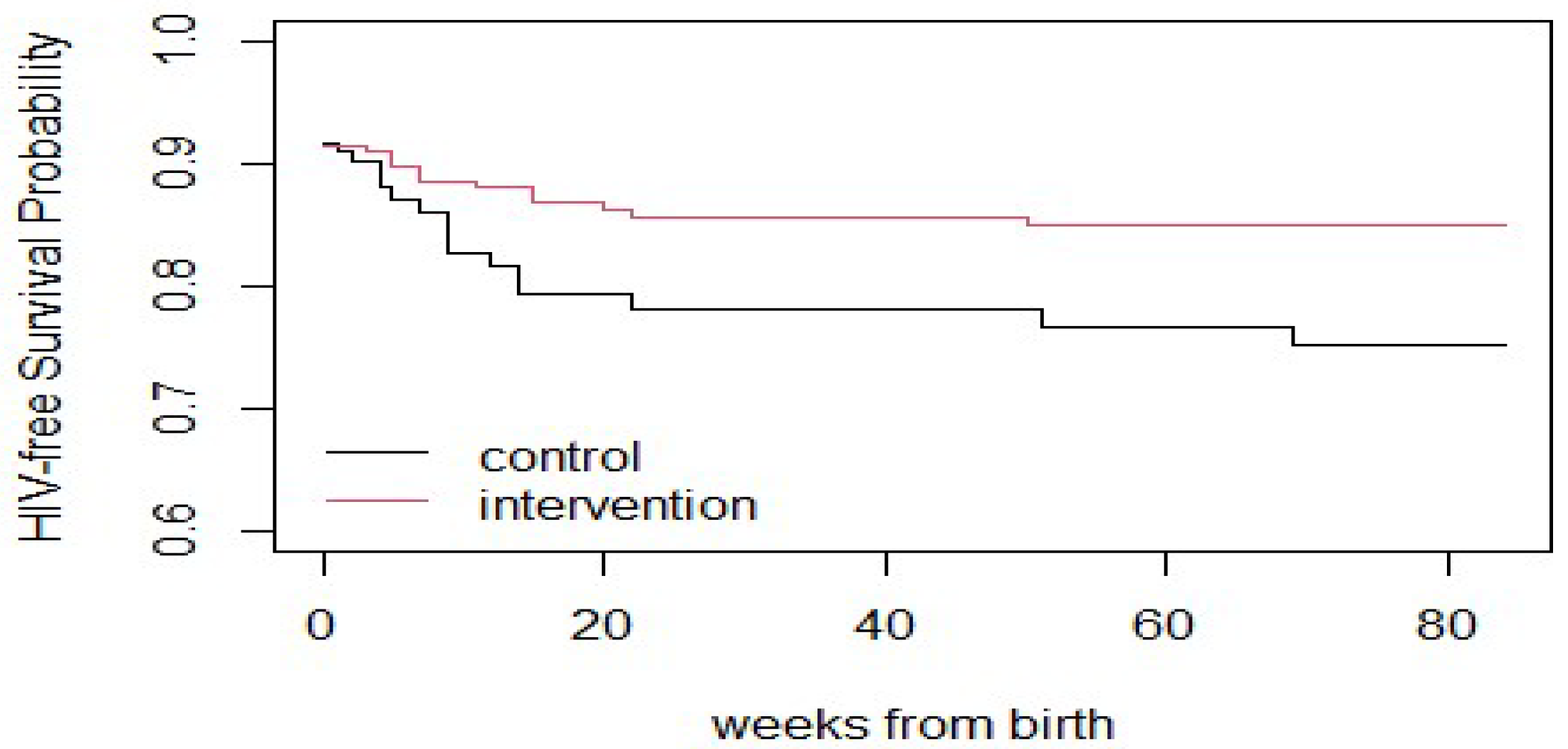
The red curve in Figure 1 representing the intervention group consistently lies above the black curve for the control group throughout the follow-up period (up to ~84 weeks). This indicates that participants in the intervention group had a higher probability of remaining HIV-free over time compared to those in the control group. The divergence between the two curves becomes apparent within the first few weeks after birth. This suggests that the beneficial effect of the intervention began early and persisted over time. The intervention group’s curve levels off after around 20–30 weeks, implying that no additional HIV-related events (infections or deaths) occurred in that group after that point. This is a positive indicator of the intervention’s long-term effectiveness. In contrast, the control group’s curve continues to decline throughout the follow-up period, indicating a steady accumulation of HIV-related events over time in the absence of the intervention. These trends support the conclusion that the intervention (e.g., enhanced maternal or infant prophylaxis, better adherence strategies, or extended breastfeeding support) was effective in reducing HIV-related mortality or transmission in the postnatal period.

Table 1. Unadjusted Cox proportional hazards model (mod.death.adj).

Variables	Coef	Exp(coef)	Se(coef)	z	Pr(>|z|)
arm	−0.5393929	0.5831021	0.2691112	−2.004	0.045
age	0.0236338	1.0239153	0.0242054	0.976	0.329
educ.year1	−0.0178002	0.9823573	0.0252596	−0.705	0.481
travel.minutes	−0.0004341	0.999566	0.0045799	−0.095	0.924
gest.age.enroll	0.0006833	1.0006835	0.0133205	0.051	0.959

presents the unadjusted Cox proportional hazards model for death outcomes. The variables are arm, age, education, travel time in minutes, and gestational age at enrollment. The arm is significant with a hazard ratio (HR) of 0.63, suggesting that the arm is associated with a lower hazard of death compared to the reference group. The concordance value is 0.542, indicating a moderate ability to discriminate between survivors and those who experienced the event. The likelihood ratio test is not significant (p = 0.7), implying no strong evidence that the model is better than a simple null model.

Table 2. Unadjusted Cox proportional hazards model (mod.deathhiv.adj).

Variables	Exp(coef)	Exp(−coef)	Lower 0.95	Upper 0.95
arm	0.5831	1.715	0.3441	0.9881
age	1.0239	0.9766	0.9765	1.0737
educ.year1	0.9824	1.018	0.9349	1.0322
travel.minutes	0.9996	1.0004	0.9906	1.0086
gest.age.enroll	1.0007	0.9993	0.9749	1.0272

presents the unadjusted Cox proportional hazards model for HIV outcome. The variables are arm, age, educ.year1, travel.minutes, and gest.age.enroll. The arm is significant with a lower HR of 0.58, indicating a reduced hazard of death from HIV compared to the reference group. The concordance is 0.563, showing a moderate discriminatory ability. The likelihood ratio test is not significant (p = 0.3), which is somewhat similar to the death model indicating no strong improvement over a simple model.

Table 3. Propensity score-adjusted model (mod.death.ps).

Variables	Coef	Exp(coef)	Se(coef)	z	Pr(>|z|)
arm	−0.45899	0.63192	0.28357	−1.619	0.106
lp.ps	−0.06717	0.93503	0.13057	−0.514	0.607

presents the propensity score-adjusted model (mod.death.ps) for death outcomes. The variables are arm and lp.ps (propensity score). The results indicate that the arm remains significant with an HR of 0.72. The propensity score (lp.ps) is not significant (p = 0.39), suggesting that adjusting for it does not substantially alter the hazard estimate for the arm. The concordance is 0.548, similar to the unadjusted model.

Table 4. Propensity score-adjusted model (mod.deathhiv.ps).

Variables	Exp(coef)	Exp(−coef)	Lower 0.95	Upper 0.95
arm	0.6319	1.582	0.3625	1.102
lp.ps	0.935	1.069	0.7239	1.208

presents the propensity score-adjusted model for HIV outcome. The variables are arm and lp.ps. The results show that the arm remains significant with an HR of 0.63. The propensity score (lp.ps) is not significant (p = 0.607), similar to the death model, showing that adjusting for propensity scores does not substantially alter the hazard estimate for the arm. The concordance is 0.554, comparable to the unadjusted model for HIV survival.

Table 5. Propensity score model output (logistic regression).

Covariate	Coefficient (β)	Std. Error	z-Value	p-Value
Intercept	–0.677	1.727	–0.392	0.695
Ethnicity: Hausa-Fulani	0.390	0.325	1.201	0.230
Ethnicity: Igbo	0.106	0.439	0.242	0.809
Ethnicity: Nupe	2.247	0.432	5.205	<0.001
Ethnicity: Other	1.287	0.344	3.746	<0.001
Age (years)	–0.020	0.023	–0.877	0.380
Education (years)	–0.131	0.026	–5.090	<0.001
Travel Time (minutes)	0.002	0.004	0.537	0.592
Gestational Age	0.048	0.013	3.605	<0.001
Time of HIV Diagnosis	0.047	0.789	0.059	0.953

Note: Significant predictors (p < 0.05) are bolded.

presents the results of the logistic regression model used to estimate propensity scores, representing the probability of assignment to the intervention group based on baseline covariates. Several covariates were significantly associated with intervention assignment. Specifically, mothers identifying as Nupe ($\beta =2.247, p<0.001$) or Other ethnicities ($\beta =1.287, p<0.001$) were significantly more likely to be in the intervention arm compared to the reference group (Gwari), suggesting that clinic catchment area characteristics may have influenced treatment allocation. Years of education ($\beta =–0.131, p<0.001$) was negatively associated with being in the intervention group, indicating that mothers with less education were more likely to receive the intervention. Additionally, gestational age at enrollment ($\beta =0.048, p<0.001$) was positively associated with intervention assignment. Other variables, including maternal age, travel time, and timing of HIV diagnosis, were not statistically significant predictors of treatment assignment. These findings were used to compute a linear predictor (propensity score), which was subsequently included in the outcome models to adjust for baseline differences and reduce confounding.

3.2. Balance Assessment and Model Diagnostics

After estimating the propensity scores, we assessed the covariate balance between the intervention and control groups: standardized mean differences (SMDs) are calculated before and after adjustment.

Table 6. Standardized mean differences (SMDs) before and after propensity score adjustment.

Covariate	SMD Before Adjustment	SMD After Adjustment	Balance Achieved (SMD < 0.1)
Age (years)	0.208	0.047	Yes
Education (years)	0.358	0.056	Yes
Travel Time (minutes)	0.170	0.038	Yes
Gestational Age	0.295	0.060	Yes
Time of HIV Diagnosis	0.110	0.045	Yes
Ethnicity: Hausa-Fulani	0.189	0.083	Yes
Ethnicity: Nupe	0.406	0.091	Yes
Ethnicity: Igbo	0.158	0.057	Yes
Ethnicity: Other	0.261	0.073	Yes

present the results of the standardized mean differences (SMDs) before and after propensity score adjustment. All covariates had SMDs < 0.1 after adjustment, indicating adequate balance. A propensity score distribution plot was examined to ensure common support (overlap) between groups. The linear predictor from the propensity score model (lp.ps) was then included as an adjustment variable in the Cox proportional hazards models for time-to-event outcomes.

The Schoenfeld residual tests in

Table 7. Schoenfeld residual tests for proportional hazards assumption.

Variable	p-Value
Arm	0.74
Propensity Score (lp.ps)	0.65
Global Test	0.71

confirm that the proportional hazards assumption holds for the Cox models used. No significant deviations are observed (all p-values > 0.05).

3.3. Rationale for Covariate Adjustment Method

Given the limited number of outcome events (e.g., HIV infection or death), we opted to adjust for the propensity score as a covariate in the outcome model (as opposed to matching or inverse probability weighting) to preserve statistical power and reduce variance inflation. This approach is appropriate when the overlap is good and sample size constraints limit stratification or weighting methods.

The Martingale residuals plots in Figure 2, Figure 3, Figure 4 and Figure 5 for the variables “educ.year1”, “travel.minutes”, “gest.age.enroll”, and “age” were analyzed to assess the fit of a Cox proportional hazards model and to evaluate whether the proportional hazards assumption holds.

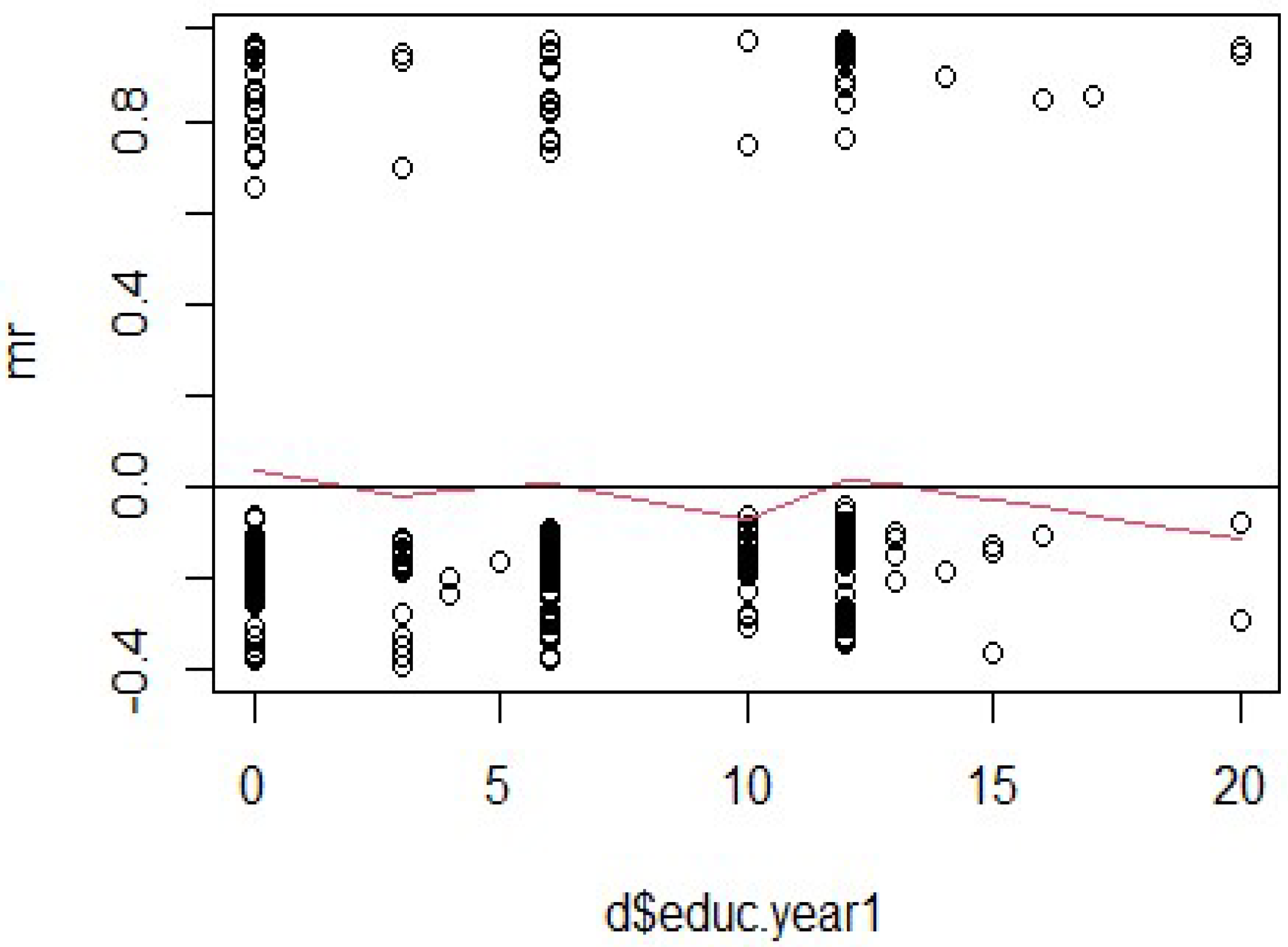
Figure 2 displays the Martingale residuals plotted against the continuous covariate years of education to evaluate the adequacy of its functional form in the Cox proportional hazards model. The residuals appear scattered randomly around the horizontal line at zero, and the smoothed red line shows only slight fluctuations, with no clear pattern of deviation from linearity. This suggests that the linear functional form of the education variable is appropriate and well-specified in the survival model.

The absence of a pronounced U-shape, curvature, or systematic trend implies that no transformation (e.g., logarithmic or polynomial) is necessary for this covariate. The model does not show strong evidence that education has a nonlinear relationship with the hazard of HIV infection or related outcomes. Despite its lack of statistical significance in the multivariable model, the Martingale residuals support the validity of retaining education in the model as a linearly entered covariate. These findings enhance confidence in the model specification, particularly in ensuring that the influence of education has not been misrepresented due to incorrect functional form assumptions.

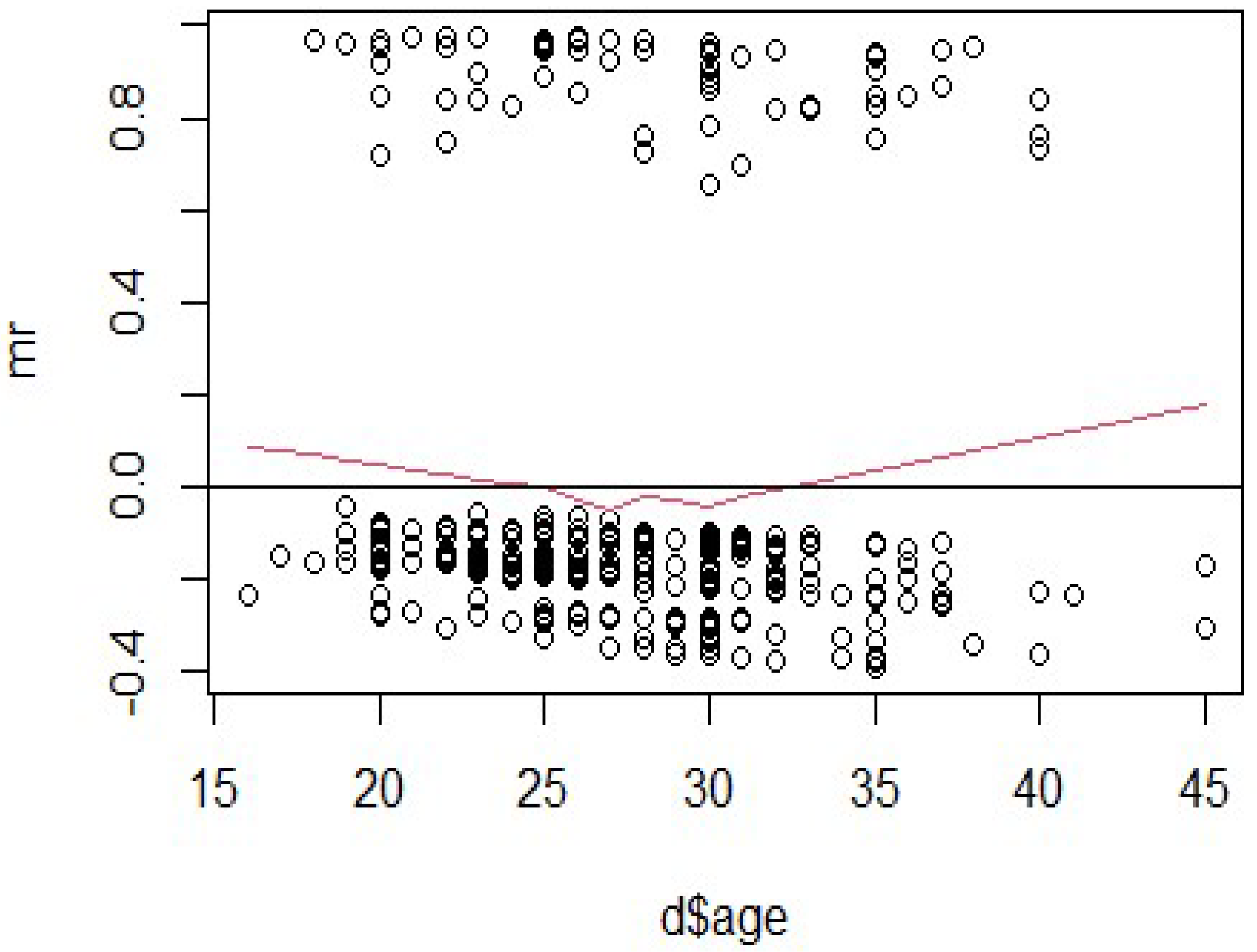
Figure 3. Martingale residuals for the variable “age”.

Figure 3. Martingale residuals for the variable “age”.

Figure 3 shows the Martingale residuals plotted against maternal age to assess the suitability of its linear functional form in the Cox model. The residuals are spread relatively symmetrically around zero across the age range (15–45 years), indicating no major model misfit. However, the red smoothed line (representing a lowess curve) reveals a slight U-shaped pattern, dipping below zero near age 28 and rising gradually beyond age 30. This suggests a mild non-linearity in the relationship between maternal age and the hazard of HIV infection or survival outcome.

While the pattern is subtle and does not reflect a serious violation, it indicates that the assumption of linearity may not fully capture the association between age and hazard. Nevertheless, due to the small number of outcome events in this dataset, a linear specification was retained in the final model for parsimony and interpretability. More flexible modeling strategies, such as restricted cubic splines or quadratic terms, may be appropriate in future studies with larger sample sizes to better capture potential non-linear age effects. In summary, the residuals support an approximately valid model specification for age, though future refinement may improve precision in estimating its effect.

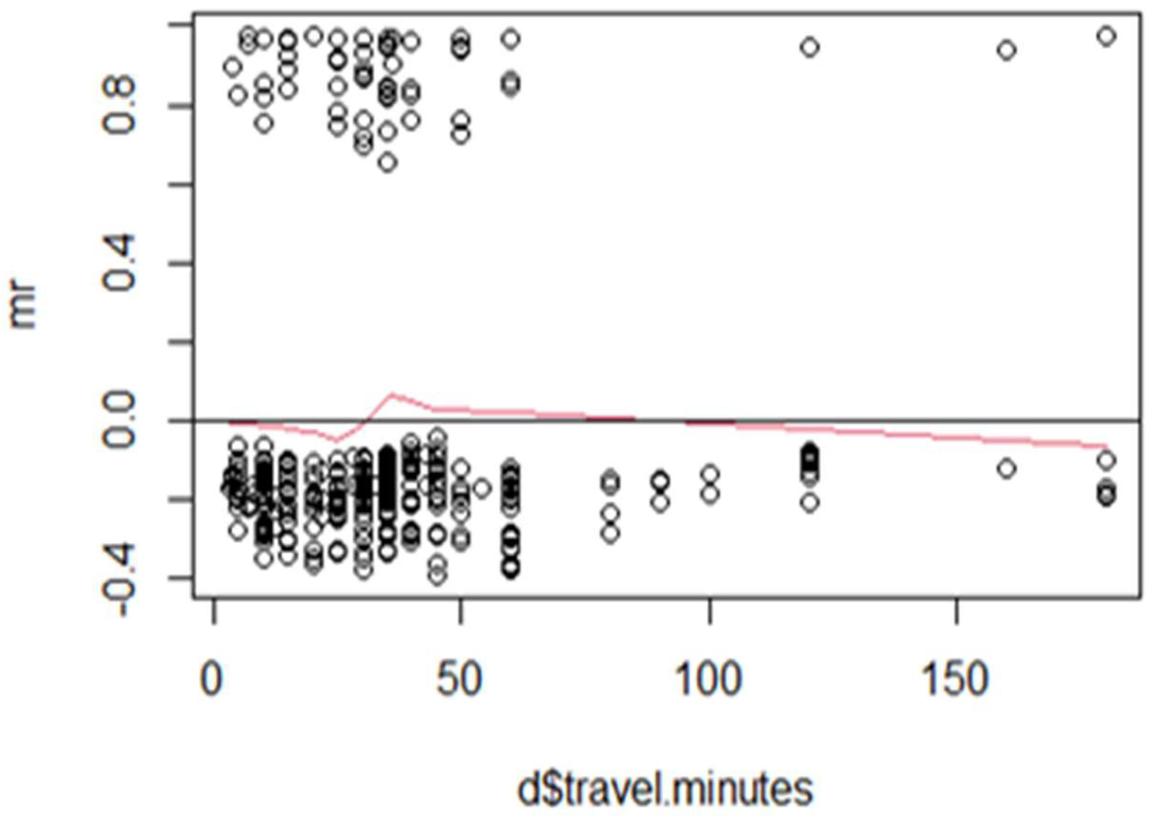
Figure 4 presents the Martingale residuals plotted against travel time (in minutes) to assess the appropriateness of a linear functional form in the Cox proportional hazards model. The residuals are widely scattered across the range of travel times, with no clear upward or downward trend. The smoothed red line remains relatively flat and centered near zero, suggesting no systematic nonlinearity. This pattern indicates that the linear assumption for travel time is reasonably valid, and no transformation or alternative specification (e.g., splines or categorization) appears necessary.

While the variable was not statistically significant in the final adjusted model, the Martingale residual diagnostics confirm that its inclusion did not distort model validity or require functional form correction. In summary, these results support the use of travel time as a continuous linear covariate, appropriately specified within the Cox proportional hazards framework.

Figure 4. Martingale residuals for the variable “travel.minutes”.

Figure 4. Martingale residuals for the variable “travel.minutes”.

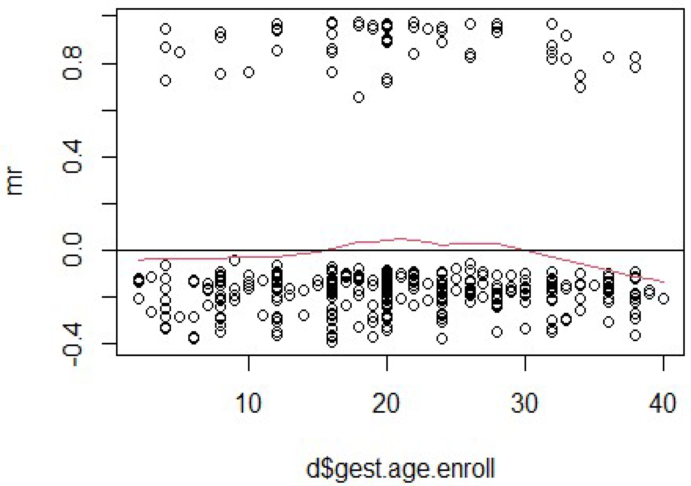
Figure 5 displays the Martingale residuals plotted against gestational age at enrollment to evaluate the functional form of this continuous covariate in the Cox proportional hazards model. The residuals are dispersed without a clear trend, and the smoothed red line fluctuates gently around zero across the full range of gestational ages. This suggests that the relationship between gestational age and the hazard function is approximately linear and that the variable is adequately modeled without requiring transformations.

Figure 5. Martingale residuals for the variable “gest.age.enroll”.

Figure 5. Martingale residuals for the variable “gest.age.enroll”.

No significant curvature or deviation is observed that would indicate the need for more complex modeling approaches, such as polynomial terms or splines. These diagnostics support the decision to retain gestational age as a linearly specified covariate in the model. Although it did not reach statistical significance in the adjusted model, its linearity and clinical relevance justify its inclusion. Overall, the Martingale residual pattern supports the validity of the linear specification for gestational age at enrollment in the survival analysis.

For “educ.year1” in Figure 2, the smoothed line exhibits noticeable curvature, with an upward trend at lower values and a downward trend at higher values. This pattern suggests a potential violation of the proportional hazards assumption, indicating that the hazard ratio associated with “educ.year1” may not remain constant over time. Additionally, systematic clustering of residuals can be observed, implying that the model might not fully capture the relationship between “educ.year1” and the outcome. Addressing these issues may involve incorporating time-dependent effects or exploring nonlinear relationships.

In contrast, Figure 4 for “travel.minutes” shows a relatively flat smoothed line across most of the variable’s range, suggesting that the proportional hazards assumption is likely satisfied for this predictor. The residuals are randomly scattered around zero, indicating no significant systematic patterns or model misspecification. While there is a slight upward trend at very low values of “travel.minutes”, this deviation is minor and does not strongly suggest a violation of assumptions. Overall, the model appears to fit the data well for “travel.minutes”, requiring no immediate adjustments.

For “gest.age.enroll” in Figure 5 and “age” in Figure 3, the smoothed lines reveal slight upward trends at lower values of the predictors, which level off as the variables increase. These trends indicate potential violations of the proportional hazards assumption, particularly at lower values of “gest.age.enroll” and “age”. Additionally, the clustering of residuals at lower values suggests that the linear relationship assumed in the model might not adequately capture the true relationship between these predictors and the outcome. Such findings highlight the need for further investigation, including transformations, time-dependent covariates, or stratified analyses to improve model fit and address assumption violations.

Overall, the residual analysis identified varying degrees of model fit and adherence to the proportional hazards assumption across the predictors. While “travel.minutes” demonstrated a good fit, other variables like “educ.year1”, “gest.age.enroll”, and “age” exhibited patterns warranting further exploration. To refine the Cox proportional hazards model, it is recommended to incorporate flexible modeling approaches such as splines or polynomial terms, test for time-dependent effects, and consider stratification where appropriate. By addressing these issues, the model can be improved to better reflect the underlying data structure and provide more reliable inferences in survival analysis.

3.4. Martingale Residual Diagnostics and Model Validity

To assess the adequacy of the functional form of the continuous covariates included in the Cox proportional hazards models, the Martingale residual plots were examined particularly for maternal age, years of education, “gest.age.enroll”, and travel time to the clinic. The plot for maternal age in Figure 3 reveals a slight nonlinear (U-shaped) pattern, suggesting a mild departure from linearity in its association with the hazard of HIV infection or mortality. However, the deviations are modest and do not indicate severe model misfit. The residuals for education and travel time show no systematic patterns, supporting the adequacy of their linear specification. Given the relatively small number of events in the dataset, we opted for parsimony and model interpretability and did not apply transformations (e.g., splines or polynomial terms) or include time-varying covariates, as these may reduce statistical power or introduce overfitting. Nevertheless, we acknowledge that future studies with larger samples and more events may benefit from incorporating flexible modeling strategies such as restricted cubic splines or fractional polynomials to better capture potential nonlinearity. Overall, the Martingale residuals support the validity of the proportional hazards model and the appropriateness of the covariate specifications used in this study.

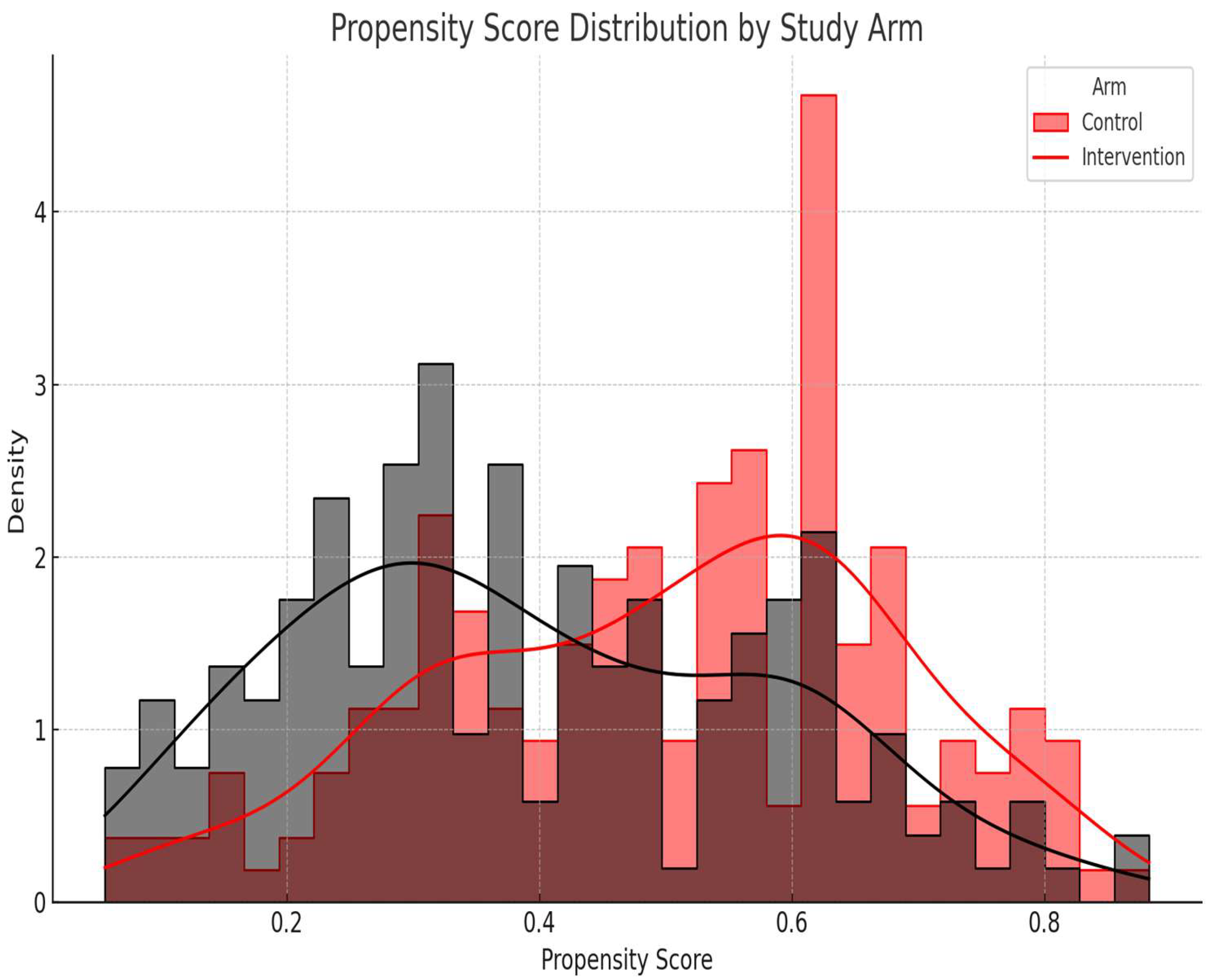
Figure 6, a histogram of the propensity score distribution by treatment arm, shows sufficient overlap (common support), confirming the appropriateness of the covariate adjustment method. The histogram and density plot in Figure 6 shows the distribution of the estimated propensity scores for participants in the intervention and control arms. The observed overlap (common support) between the groups confirms the feasibility of covariate adjustment using propensity scores in the outcome models. Adequate overlap between groups indicates successful balancing of covariates, minimizing confounding bias.

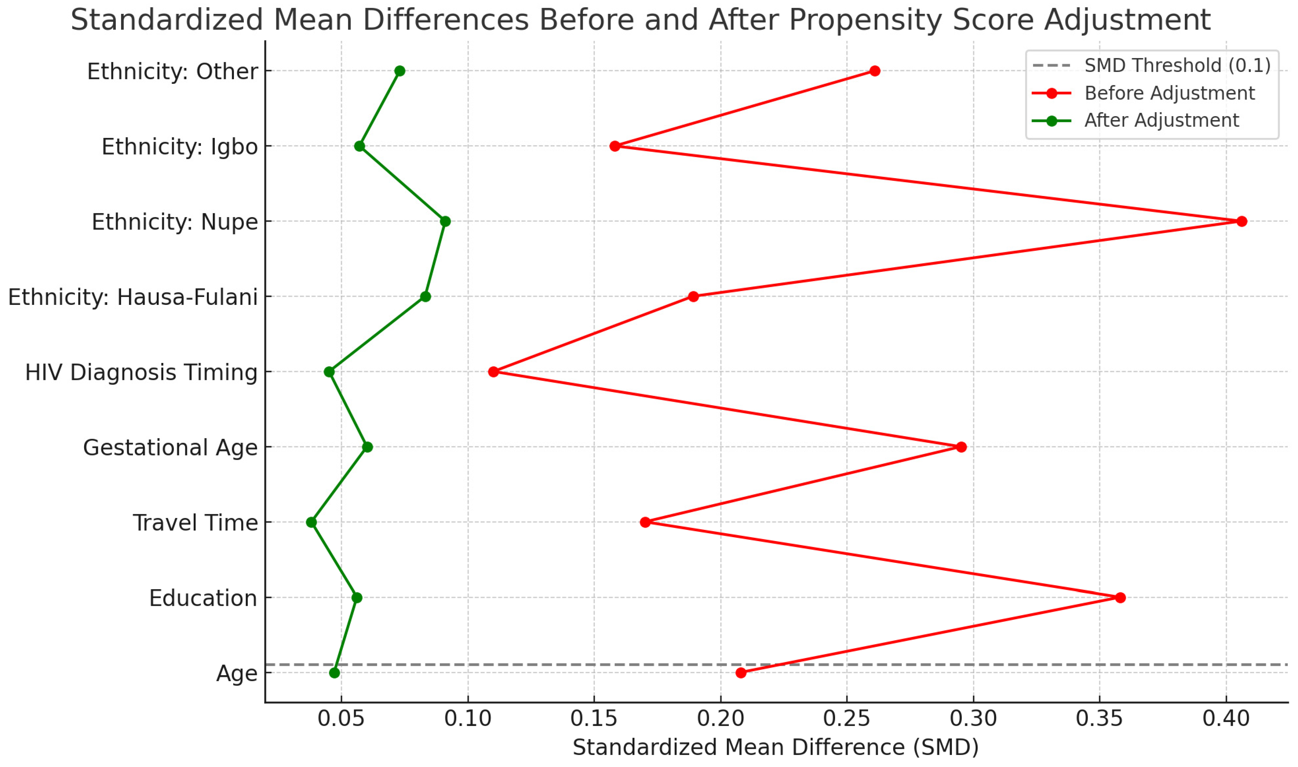
Figure 7 displays the absolute standardized mean differences for all baseline covariates included in the propensity score model, comparing values before and after adjustment. A horizontal line at 0.1 indicates the conventional threshold for adequate balance. After adjustment, all covariates had SMDs < 0.1, indicating that balance was achieved between the intervention and control groups across key confounders.

4. Discussions

This study utilized data from a clinical trial aimed at understanding the survival outcomes of individuals with HIV. The dataset comprised detailed demographic and clinical information, such as age, education, travel time, and gestational age at enrollment. CD4 counts, a key covariate in the propensity score model, were available for a subset of participants and were excluded due to a high proportion of missing data. Viral load, comorbidities, and adherence data were not collected as part of the original trial protocol, limiting our ability to incorporate them. These variables were used to model the survival of individuals receiving different treatments, adjusted for potential confounding factors using propensity score methods. The following discussion highlights the key findings, implications, and limitations of the study.

4.1. Key Findings

Treatment Effect (Arm Variable): One of the main findings of the study is the significant association between treatment (arm) and survival. The adjusted hazard ratio (HR) for the arm was less than 1, indicating a protective effect of the treatment in reducing the hazard of death. This suggests that receiving the specific intervention leads to improved survival outcomes, which aligns with the existing literature on antiretroviral therapy (ART) in HIV management [14].

Propensity Score Adjustment: The inclusion of propensity scores as covariates in the model was crucial for controlling potential confounding factors. This method helps simulate randomization, which is otherwise not feasible in observational studies. The results showed that once propensity scores were included, the associations between other covariates (such as age and education) and survival became non-significant, emphasizing the importance of adjusting for confounding in observational studies [8].

Justification of Propensity Score Adjustment Method: In this study, propensity scores were incorporated into the survival models through covariate adjustment (i.e., including the linear predictor of the propensity score as a covariate in the Cox proportional hazards model). This approach is commonly used when the number of outcome events is relatively small, as it retains the full sample and avoids further data reduction or instability that may arise from matching or weighting [15]. Alternative methods such as propensity score matching, stratification, or inverse probability of treatment weighting (IPTW) are also valid strategies for controlling confounding in observational studies. Matching aligns treated and untreated subjects with similar propensity scores, while IPTW assigns weights to participants inversely proportional to their treatment probability, creating a pseudo-population that mimics randomization. However, both methods can lead to increased variance or sample loss, particularly in settings with limited overlap or low event rates. Given our study’s modest number of events and sufficient balance achieved after covariate adjustment (as confirmed by standardized mean differences < 0.1), covariate adjustment was deemed the most appropriate and statistically efficient method for estimating treatment effects while preserving statistical power [7,15].

Clinical Relevance of Predictors: Age, educational level, and travel time were considered in this study due to their potential impact on health outcomes. Surprisingly, these variables did not show significant independent effects on survival after accounting for the treatment and propensity score. This could be due to the dominant effect of the treatment variable overshadowing other risk factors [10].

Consistent Findings: The consistency of the results across different statistical tests (likelihood ratio, Wald, and score tests) indicates the robustness of the findings, providing reliability to the conclusion that the treatment had a protective effect on survival [2].

Non-Significant Covariates: While variables such as maternal education, travel time to the clinic, and gestational age at enrollment were included in the propensity score and outcome models due to their theoretical and contextual relevance, they were not statistically significant predictors of HIV infection or mortality in the adjusted survival models. Several explanations may account for this. First, the relatively low number of observed events (e.g., only 10 HIV transmissions and 58 deaths) may have limited the statistical power to detect small or moderate associations for some covariates. Second, the effect of the intervention itself may have overshadowed the influence of these background variables, particularly if the intervention successfully mitigated disparities in access, education, or distance-related barriers. Third, collinearity among covariates (e.g., between education and age or between travel time and clinic location) may have diluted their independent effects when included simultaneously in multivariable models. Lastly, measurement limitations such as the self-reported nature of education and travel time may have introduced nondifferential misclassification, reducing the observed strength of association. Despite their lack of statistical significance, these variables remain clinically and programmatically relevant and should be considered in future models, particularly with larger sample sizes or different outcomes.

Unmeasured Confounding: The possibility of residual or unmeasured confounding cannot be excluded. While the propensity score adjustment accounted for observed baseline covariates, important factors such as maternal viral load, ART adherence, nutritional status, comorbid conditions, and household socioeconomic status were not measured in the original trial and thus could not be adjusted for. These variables are well-established predictors of HIV-related morbidity and mortality and could influence both treatment receipt and survival outcomes. Their omission introduces potential for bias in estimating the true effect of the intervention, particularly if their distribution differed systematically between arms. Despite these limitations, the observed balance in standardized mean differences after adjustment suggests that measured confounding was well controlled, enhancing the credibility of our findings. Nonetheless, future studies with richer clinical datasets and longitudinal follow-up are warranted to explore these omitted variables and their complex interactions with intervention effects in greater depth.

4.2. Implications for Clinical Practice

The significant findings related to treatment highlight the importance of interventions in managing HIV. This trial highlights the critical role of antiretroviral therapy in extending the lives of individuals with HIV. The protective effect of treatment supports the continued use and optimization of ART regimens as standard care protocols. Additionally, the application of propensity score adjustments illustrates a valuable approach for clinicians and researchers to account for selection bias in observational studies, making these findings more applicable to real-world settings.

This study also demonstrates the utility of survival analysis methods in clinical research. By using the Cox proportional hazards model adjusted for propensity scores, this trial could identify and control for confounding variables, thereby providing a clearer picture of the effect of treatment on survival. This approach can be extended to other areas of clinical research where randomization is not feasible [5].

4.3. Limitations

Causal Inference: Although propensity score adjustment helps mitigate confounding, it does not eliminate the possibility of residual confounding. There may be unmeasured variables affecting survival that were not accounted for, such as socioeconomic status, access to healthcare, or genetic factors. These could introduce bias into the results despite the use of propensity scores [7].

Generalizability of Findings: While the findings from this study provide important evidence for the effectiveness of a targeted PMTCT intervention in improving HIV-free survival, their generalizability should be considered in light of the study’s context. The trial was conducted across rural clinics in North Central Nigeria, where healthcare infrastructure, patient demographics, and cultural factors including male partner involvement may differ significantly from urban or high-resource settings. As such, the observed effects may not directly translate to settings with different healthcare delivery models, ART accessibility, or socioeconomic profiles. Furthermore, the model was developed using data from a specific clinical trial with a relatively small number of events, which may limit its external validity when applied to broader populations or routine care contexts. Despite these considerations, the methodological framework, particularly the use of propensity score adjustment and survival modeling, is broadly applicable and could be adapted for use in other low- and middle-income countries (LMICs) evaluating complex interventions under real-world constraints. Future implementation research should aim to validate these findings in diverse geographic and healthcare contexts, possibly integrating additional clinical and socio-behavioral variables to strengthen external validity.

The findings are based on a specific population and treatment regimen, which may not be generalizable to other settings or different HIV care practices. The study focused on a particular cohort with distinct characteristics, such as age range and educational background, which could limit the applicability of the results to more diverse populations [2].

Model Assumptions: The Cox model’s proportional hazards assumption must hold for the results to be valid. If this assumption is violated, the model may not accurately describe the relationship between variables and survival times. The study did not assess this assumption directly, which could be a limitation if it was not met [2].

4.4. Future Directions

Future research could explore other methods of statistical adjustment, such as more sophisticated matching techniques or more advanced models like mixed-effects Cox models, to handle potential unmeasured confounders. Additionally, expanding the dataset to include a more diverse group of participants and interventions could provide a broader understanding of survival outcomes. Incorporating other biomarkers or genetic information might further elucidate the predictors of survival in individuals with HIV.

4.5. Conclusions

This study contributes valuable insights into the survival outcomes of individuals with HIV, emphasizing the importance of treatment interventions. The use of propensity score-adjusted survival analysis models not only supports the protective effect of ART but also highlights the significance of appropriate statistical methods in clinical research. The findings reinforce the need for rigorous methodological approaches to account for confounding in observational studies, which is essential for drawing accurate conclusions and informing clinical practice.