Abstract
The fundamental problem with causal inference involves discovering causal relations between variables used to describe observational data. We address this problem within the formalism of information field theory (IFT). Specifically, we focus on the problems of bivariate causal discovery (X → Y, Y → X) from an observational dataset . The bivariate case is especially interesting because the methods of statistical independence testing are not applicable here. For this class of problems, we propose the moment-constrained causal model (MCM). The MCM goes beyond the additive noise model by exploiting Bayesian hierarchical modeling to provide non-parametric reconstructions of the observational distributions. In order to identify the correct causal direction, we compare the performance of our newly-developed Bayesian inference algorithm for different causal directions (, Y → X) by calculating the evidence lower bound (ELBO). To this end, we developed a new method for the ELBO estimation that takes advantage of the adopted variational inference scheme for parameter inference.
1. Introduction
Since Pearl’s pioneering works on causality [1,2], various new methods have been developed for the study of causal inference (for example, see [3] for a complete overview). In particular, the case of bivariate causal inference remains of central interest because the traditional interventional methods are not applicable in this regime. The problem of inferring causal relations from observational data is usually tackled following one of three main approaches [4]. In the first approach, often referred to as the constraint-based approach, the correct causal graph is identified by analyzing conditional independence in the observational data distribution [5,6,7]. Methods that follow this approach can recover the true causal directed acyclic graph (DAG) up to its Markov equivalence class under some technical assumptions, but are inapplicable in the bivariate case, where no conditional-independence relationship is available.
The second approach, referred to as the score-based approach, fits the observational data by searching in the space of all possible DAGs of a given size and assigning a score to the result. This score is used to infer the correct causal relations [8], but again can only identify the causal graph up to its Markov equivalence class. Therefore, both constrained-based and score-based methods are not suited to perform causal inference in the bivariate case. However, combined constraint and score-based approaches that use generative neural networks (see Goudet et al. [9]) are also able to infer causal directions in the bivariate case.
The third and final approach is the asymmetry-based approach. Asymmetry-based methods exploit the asymmetries between the cause and the effect variables to reconstruct the underlying causal relations. These methods either evaluate the algorithm complexity of the two possible conditional distributions X → Y and Y → X resulting from splitting the joint probability density given a model [10,11,12,13] or check for the independence of the conditional probability of the effect given the cause from the cause’s independent probability distribution (information geometric causal inference [14,15]). This work most resembles the asymmetry-based approach described above. Here, we continue the series of works [16,17] that exploit the Information Field Theory (IFT) formalism [18,19,20,21] for causal inference, with two important novelties. First, we use the geometric variational inference (geoVI) approach as the inference tool for our hierarchical model. This has the advantage that the final covariance estimate of the posterior is better tailored to the problem and therefore for our evidence estimation, described in Section 3.7. Second, we propose a new causal model that can extend beyond the additive noise models (ANMs) formulation and allow for more flexible noise parameterization, while explicitly breaking the symmetry between cause and effect (Section 3.3).
2. Causal Inference and Bayesian Generative Models
In this section, we state the bivariate problem (Section 2.1), make a connection to the IFT formalism (Section 2.2), and then introduce structural causal models (SCMs) (Section 2.3).
2.1. The Bivariate Problem
The bivariate problem is of central importance in causal inference. Given a DAG representing a causal relation between N random variables , the joint distribution factorizes as
which is the Markov condition described by Pearl [1]. In fact, this shows that if we can characterize this factorization in such a way that the conditional probabilities are “smoother” or “simpler” for the true causal direction, we can recover the complete causal graph [13,22]. For this reason, i.e., to determine the correct causal structure of a complicated DAG, we only need to determine the parent cause direction, we can restrict ourselves to the bivariate X → Y and Y → X problems. The bivariate problem can be stated as follows. Given a dataset formed by pairs composed by realizations and of the random variables X and Y, respectively, predict the underlying causal direction choosing between X → Y or Y → X.
2.2. Causal Inference and IFT
We note that the structure of Equation (1) resembles Bayesian hierarchical generative modeling. This similarity is made even stronger if we consider the so-called structural causal models (SCMs) (see Section 6.2 of [3,23]). The SCM is composed of a DAG, which uniquely identifies the causal directions between a set of given variables, and a function f, which we refer to as the causal mechanism, and which links the causes to their effects within the DAG. In addition to the cause–effect pairs, the SCM is also supplemented by a set of noise variables . Then the bivariate problem can be stated as
Under certain conditions, this relation can uniquely identify the correct causal mechanism [1]. We stress how Equation (2) can easily be represented by a hierarchical generative model, once the split from Equation (1) is given. Since generative models can be directly related to inference (see, e.g., Enßlin [21]), we will use the framework of information field theory (IFT). IFT is Bayesian inference for the fields. Here, the fields we need to infer from noisy data are the probability distributions of X, Y, and their conditionals, given some model . For details on our inference scheme, we refer to Section 3.6. The problem of detecting the true underlying causal direction reduces to probing all possible splits in Equation (1) and selecting the one with the highest score, given by our evidence estimate (see Section 3.7).
2.3. SCMs and Bayesian Generative Modeling
Combining Bayesian generative modeling and IFT, it is possible to reproduce complicated densities non-parametrically, given some prior assumptions on their smoothness [24,25]. As discussed in Section 1, some asymmetry-based models, including the novel causal model we propose in this work (Section 3.3), exploit the idea that the conditional distributions are somewhat “simpler” in the correct causal direction. It is then natural to generate these probability distributions directly and then try to find their correspondent SCMs. In particular, if we want to produce the conditional distribution for the X → Y causal direction, we need to define a model to generate X → Y. We can then relate this distribution to an SCM of the form described in Equation (2) by considering
where we denote with the distribution of the noise variable , with the inverse with respect to the second argument of , such that , and with Dirac’s delta distribution. We note that without loss of generality, we can choose the noise variable to be uniformly distributed over its domain invoking the inverse cumulative distribution function (inverse CDF) method. We can then absorb the inverse CDF transformation into f. In this parameterization, Equation (3) reduces to
3. From Additive Noise Models to MCM
In this section, we give an overview of the additive noise model (ANM) as a paradigmatic example of a simple asymmetry method and the flexible noise model (FNM) as a more complicated one. We then propose a novel causal model that can overcome some of their limitations.
3.1. The Additive Noise Model
From the very definition of the SCM, it might be reasonable to model the effect of a cause variable X on a variable Y through a deterministic causal mechanism f plus independent noise . Such a model is called Additive Noise Model (ANM) [11,23]. In the linear, non-Gaussian, and acyclic models (LiNGAM, see Shimizu et al. [26]), f is linear, and at most one variable between X or is normally distributed. In the nonlinear ANM proposed by Hoyer et al. [11], f is nonlinear and the only constraint on the noise distribution is to be independent of the cause X.
Mimicking the approach followed in Section 2.3, we find the ANM’s correspondent conditional density distribution. The generic additive noise model can be written in the form ; hence,
where is the distribution of the noise variable . This shows that the conditional probability for an ANM, given a specific causal direction, is the noise distribution evaluated at the residuals coordinates , for the X → Y causal direction. If we furthermore assume the noise to be normally distributed, with a fixed variance , this further reduces to the Gaussian distribution
3.2. Flexible Noise Model
Many attempts have been made to go beyond the additive noise formulation (see, e.g., [9,27]) and many algorithms have proven effective, even if they have not been directly related to SCMs. Some of these approaches have identified preferred causal directions by comparing complexity measures of the conditional distributions X → Y) and Y → X) (see, e.g., Sun et al. [13,22].). Unfortunately, in many cases, the proposed complexity measures are intractable and hard to quantify. In Guardiani et al. [25], we presented a hierarchical generative model that exploits prior information on the observed variables to produce a joint distribution, parametrized as follows
In the following, we will refer to this model as the flexible noise model (or FNM). In the FNM, the true causal direction is determined by comparing Bayesian evidence (more specifically the lower bounds of the evidence) between different possible causal graphs. As we will discuss in Section 3.7, using conditional–probability model evidences to determine causal directions inherently relates to the complexity of the conditional distribution. Intuitively, the evidence accounts for how many degrees of freedom (read algorithmic complexity) need to be excited in order to reproduce a certain joint distribution given a specific causal direction. The generative nature of Bayesian hierarchical models also allows for an understanding of these models from the SCM perspective, in which Pearl’s do-calculus, interventions, and counterfactuals are naturally defined. If we use Equation (3) for the FNM, we can describe the conditional probability of the X → Y model as
which is subject to the constraint .
While this approach is effective when prior knowledge (regarding the distributions of the observational variables) is accessible, the constraints on f are too weak to guarantee identifiability in a more general setting. In the case that no prior information on the observed variables is available and the conditional distributions are similarly complex in either causal direction, additional asymmetry must be introduced in the model in order to identify the correct causal structure.
3.3. From FNM to First-Order MCM
In the spirit of breaking the symmetry in the split of the joint distribution , we introduce the moment-constrained causal model (MCM). This model can be seen as a generalization of the nonlinear additive noise model and a (restrictive) modification of the flexible noise model. Starting from the FNM conditional distribution Equation (5), we can represent an x-independent y distribution
by setting . Then we realize that the conditional probability of the ANM from Equation (4) can simply be represented from the x-independent probability distribution in Equation (8)
if we substitute and require that g is quadratic ().
Equation (9) directly shows that a nonlinear ANM can be interpreted as a coordinate transformation that shifts the mean of a normal and zero-centered y-distribution (with fixed variance) by a nonlinear x-dependent function . We will use this intuition to develop the MCM. We now want to extend the ANM in a way that allows for more complicated noise distributions and noise-cause entanglements, similar to the FNM. As previously discussed though, in the absence of detailed prior knowledge the FNM is not capable of completely constraining the f of its corresponding SCM, nor it is able to impose strong constraints on the shape of the joint distribution X → Y). In particular, it is not uniquely centered around a smooth function as the ANM is.
Mimicking the approach described in Equation (9), we propose to extend the ANM with a model which is parametrized similarly to the FNM, but whose conditional distribution’s first moment is centered around a smooth function of x, which we call . To build this model, we could start from the FNM defined on some probe coordinates and perform the change of variable . This parameterization though allows for both and to represent the average . To eliminate this degeneracy, we introduce a slightly different change of variable
This way, will model the mean of the causal mechanism f and the function will model higher-order effects. This parameterization, together with the additional smoothness hypothesis on the functions and (see Section 3.6) fulfill our initial purpose of further breaking the symmetry in the joint distribution split in the two opposite causal directions X → Y and Y → X.
We will refer to the model in Equation (10) as the first-order MCM. Upon defining , we can write the conditional density of the MCM model as
where and represents the normalization term. By comparing Equations (9) and (11), we see that the in the MCM plays the same role as the in the ANM and that all the remaining contributions are modeled by .
3.4. Second-Order MCM
With the introduction of the first-order MCM, we have shown how to model a conditional distribution centered around a smooth function for the causal direction X → Y. The guiding intuition we want to bare in mind is that at least some of the moments of the effect variable, should somehow smoothly depend on the cause. In the first-order MCM, we demonstrate this dependence for the first moment. Taking this concept one step further, we can require that the variance of the MCM conditional density is represented by a smooth, strictly positive, and x-only dependent function . We do so by modifying the change of variable in Equation (10) into
where all expectation values are taken over the FNM conditional distribution . We note that all these expectation values depend on x.
3.5. Likelihood
Without loss of generality, we assume that the observational data d consists of N pairs , with , which live on some compact space . We bin the data into a fine two-dimensional grid over the x and y directions, such that
is the number of data counts within the where and are the pixel dimensions in the x and y directions. We then assume a Poisson likelihood
to compare the number of counts with the model’s expectations
where we indicate with X → Y) (or depending on the causal model at hand) the joint density of x and y. We note that if the data-generating process is unknown, selection effects and instrument responses can still imprint a wrong causal direction into the data. Even though under certain hypotheses it is still possible to recover the correct causal direction (see Bareinboim et al. and Correa and Bareinboim [28,29]), in general, this is not the case (see, e.g., Section Results in Guardiani et al. [25]). In principle, if we know how the data are measured, we can model the data generation process with an additional and independent likelihood factor .
3.6. Inference
In Section 2.2, we explain why the IFT generative model framework is particularly suited to developing causal inference methods. One of the main reasons is that it allows generating and inferring smooth probability distributions from the data d according to a certain causal model. Let us consider the causal direction X → Y. This problem then reduces to learning the joint density X → YX → Y) by inferring the correlation structure of the independent density parametrized as and of the conditional density X → Y). Upon denoting all unknown signal parameters with , the full model reads
We have denoted with (the same holds for g, h, and ) the parameters of the Matérn kernel parameterization of the power spectrum
This is the parameterization we use to infer the correlation structure of the signal fields s for each Fourier mode k. The process of generating smooth distributions with Matérn kernel correlation structures is described in more detail by Guardiani et al. [25].
We then need to infer the signal vector s. We do this by transforming the coordinates of the signal vector such that the prior on the new coordinates becomes an uncorrelated Gaussian as described by Frank et al. [30]. We note once again that this generative structure resembles the SCM. We then implement the resulting model using the Python package Numerical Information Field Theory (NIFTy [31,32,33]) and finally use NIFTy’s implementation of geometric variational inference (geoVI) [30] to draw posterior samples. In essence, the geoVI scheme finds an approximate coordinate transformation that maps the posterior distribution of the signal parameters into an approximate standard normal distribution. We refer to the bibliography for more details and benchmarks.
3.7. Evidence Estimation
In order to determine the true causal relations underlying the data, we estimate the Bayesian evidence lower bounds (ELBOs) of our models [34,35]. Since we’re using the geoVI variational inference approach described in Section 3.6, we can exploit the variational nature of our minimization scheme to estimate the ELBO. In fact, the ELBO can be related to the Kullback–Leibler divergence between the approximating distribution to the true posterior
where, as before, represents the parameterization of model degrees of freedom (signal), is the data, and represents the diagonalized metric of the posterior at the current sampling point. We have also denoted with the information Hamiltonian. The expectation value is estimated via geoVI posterior sample average. The represents the Kullback–Leibler divergence between the approximating distribution and the posterior . Given that , it is more convenient to consider only the lower bound
The causal direction with the highest ELBO on a given dataset d is our final estimated causal direction. We note that, for well-constructed models, the ELBO can quantify the complexity of the conditional probability distribution of the effect given the cause, since it inherently penalizes the excitation of model degrees of freedom (Occam’s razor principle).
3.8. Implementation
We implemented a preliminary version of the first-order MCM in Python and NIFTy. This implementation makes use of the inference machinery described in Section 3.6 to produce posterior reconstructions of the data d according to the MCM model.
An example of the MCM performance is shown in Figure 1. Even though it has so far only been tested on the bci_default dataset described by Kurthen et al. [16], from the reconstruction of the conditional density (Figure 1, middle column) it can be already seen that the symmetry between cause and effect is clearly broken. In the true causal direction, the field can capture more x-dependent structures from the data. For this case, the ELBO calculations support the correct X → Y causal-direction model by a Bayesian factor of ≈.
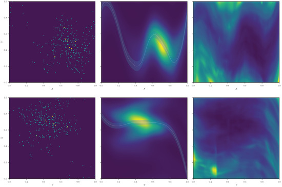
Figure 1.
Example of a preliminary implementation of the first-order MCM model on pair 0011 of the bci_default dataset. On the left, we show the raw data (counts are color-coded). In the middle, we display the reconstruction of the density as modeled by the MCM. The correspondent reconstructed field is superimposed (white dashed line, the shaded region represents one standard deviation of the geoVI posterior uncertainty). On the right, we show the relative uncertainty on . In the upper half of the figure, the causal direction is the true causal direction X → Y. In the lower half, we present the results for the wrong causal direction Y → X.
4. Conclusions
In this work, we showed the connection between SCMs and Bayesian generative modeling within the framework provided by IFT. In this spirit, we introduced a novel causal model that translates the intuition that some of the moments of the effect variable should exhibit a smooth dependence on the cause into an algorithm that explicitly breaks the symmetry in the split of the joint distribution of cause and effect. Preliminary results on a single dataset show that our new model can identify the correct causal direction. Future work directions include benchmarking first- and second-order MCM against the state-of-the-art causal inference algorithms as well as exploring possible higher-order correction terms.
Author Contributions
Conceptualization, M.G., P.F., A.K. and T.E.; methodology, M.G. and A.K.; software, M.G. and A.K.; validation, M.G.; formal analysis, M.G.; investigation, M.G. and A.K.; resources, All; data curation, M.G.; writing—original draft preparation, M.G.; writing—review and editing, M.G. and A.K.; visualization, M.G.; supervision, P.F. and T.E.; project administration, T.E.; funding acquisition, T.E. All authors have read and agreed to the published version of the manuscript.
Funding
This research was supported by the German Aerospace Center and the Federal Ministry of Education and Research through the project Universal Bayesian Imaging Kit—Information Field Theory for Space Instrumentation (Förderkennzeichen 50OO2103).
Institutional Review Board Statement
Not applicable.
Informed Consent Statement
Not applicable.
Data Availability Statement
Not applicable.
Conflicts of Interest
The authors declare no conflict of interest.
References
- Pearl, J. Models, Reasoning and Inference; Cambridge University Press: Cambridge, UK, 2000. [Google Scholar]
- Pearl, J.; Mackenzie, D. The Book of Why: The New Science of Cuse and Effect; Basic Books: New York, NY, USA, 2018. [Google Scholar]
- Peters, J.; Janzing, D.; Schölkopf, B. Elements of Causal Inference; The MIT Press: Cambridge, MA, USA, 2017. [Google Scholar]
- Mitrovic, J.; Sejdinovic, D.; Teh, Y.W. Causal Inference via Kernel Deviance Measures. In Proceedings of the NIPS’18—32nd International Conference on Neural Information Processing Systems, Montreal, QC, Canada, 3–8 December 2018; Curran Associates Inc.: Red Hook, NY, USA, 2018; pp. 6986–6994. [Google Scholar]
- Spirtes, P.; Glymour, C.N.; Scheines, R.; Heckerman, D. Causation, Prediction, and Search; MIT Press: Cambridge, MA, USA, 2000. [Google Scholar]
- Sun, X.; Janzing, D.; Schölkopf, B.; Fukumizu, K. A Kernel-Based Causal Learning Algorithm. In Proceedings of the ICML ’07—24th International Conference on Machine Learning, San Francisco, CA, USA, 24–26 October 2007; Association for Computing Machinery: New York, NY, USA, 2007; pp. 855–862. [Google Scholar] [CrossRef]
- Zhang, K.; Peters, J.; Janzing, D.; Schölkopf, B. Kernel-Based Conditional Independence Test and Application in Causal Discovery. In Proceedings of the UAI’11—Twenty-Seventh Conference on Uncertainty in Artificial Intelligence, Barcelona, Spain, 14–17 July 2011; AUAI Press: Arlington, VA, USA, 2011; pp. 804–813. [Google Scholar]
- Chickering, D.M. Optimal Structure Identification with Greedy Search. J. Mach. Learn. Res. 2003, 3, 507–554. [Google Scholar] [CrossRef][Green Version]
- Goudet, O.; Kalainathan, D.; Lopez-Paz, D.; Caillou, P.; Guyon, I.; Sebag, M. Causal Generative Neural Networks. arXiv 2017, arXiv:1711.08936. [Google Scholar]
- Hoyer, P.O.; Shimizu, S.; Kerminen, A.J.; Palviainen, M. Estimation of causal effects using linear non-Gaussian causal models with hidden variables. Int. J. Approx. Reason. 2008, 49, 362–378. [Google Scholar] [CrossRef]
- Hoyer, P.; Janzing, D.; Mooij, J.M.; Peters, J.; Schölkopf, B. Nonlinear causal discovery with additive noise models. In Advances in Neural Information Processing Systems; Koller, D., Schuurmans, D., Bengio, Y., Bottou, L., Eds.; Curran Associates, Inc.: Red Hook, NY, USA, 2008; Volume 21. [Google Scholar]
- Mooij, J.M.; Stegle, O.; Janzing, D.; Zhang, K.; Schölkopf, B. Probabilistic Latent Variable Models for Distinguishing between Cause and Effect. In Proceedings of the 23rd International Conference on Neural Information Processing Systems (NIPS’10), Vancouver, BC, Canada, 6–9 December 2010; Curran Associates Inc.: Red Hook, NY, USA, 2010; Volume 2, pp. 1687–1695. [Google Scholar]
- Sun, X.; Janzing, D.; Schölkopf, B. Causal reasoning by evaluating the complexity of conditional densities with kernel methods. Neurocomputing 2008, 71, 1248–1256. [Google Scholar] [CrossRef]
- Daniusis, P.; Janzing, D.; Mooij, J.; Zscheischler, J.; Steudel, B.; Zhang, K.; Schölkopf, B. Inferring deterministic causal relations. In Proceedings of the 26th Conference on Uncertainty in Artificial Intelligence, Catalina Island, CA, USA, 8–11 July 2010; Max-Planck-Gesellschaft; AUAI Press: Corvallis, OR, USA, 2010; pp. 143–150. [Google Scholar]
- Janzing, D.; Mooij, J.; Zhang, K.; Lemeire, J.; Zscheischler, J.; Daniušis, P.; Steudel, B.; Schölkopf, B. Information-geometric approach to inferring causal directions. Artif. Intell. 2012, 182–183, 1–31. [Google Scholar] [CrossRef]
- Kurthen, M.; Enßlin, T. A Bayesian Model for Bivariate Causal Inference. Entropy 2019, 22, 46. [Google Scholar] [CrossRef] [PubMed]
- Kostic, A.; Leike, R.; Hutschenreuter, S.; Kürthen, M.; Torsten, E. Bayesian Causal Inference with Information Field Theory. 2022; in press. [Google Scholar]
- Enßlin, T.A.; Frommert, M.; Kitaura, F.S. Information field theory for cosmological perturbation reconstruction and nonlinear signal analysis. Phys. Rev. 2009, 80, 105005. [Google Scholar] [CrossRef]
- Enßlin, T. Information field theory. In AIP Conference Proceedings; American Institute of Physics: College Park, MD, USA, 2013; Volume 1553, pp. 184–191. [Google Scholar]
- Enßlin, T.A. Information theory for fields. Ann. Der Phys. 2019, 531, 1800127. [Google Scholar] [CrossRef]
- Enßlin, T. Information Field Theory and Artificial Intelligence. Entropy 2022, 24, 374. [Google Scholar] [CrossRef] [PubMed]
- Sun, X.; Janzing, D.; Schölkopf, B. Causal Inference by Choosing Graphs with Most Plausible Markov Kernels. In Proceedings of the 9th International Symposium on Artificial Intelligence and Mathematics, Fort Lauderdale, FL, USA, 4–6 January 2006; Max-Planck-Gesellschaft: Munich, Germany, 2006; pp. 1–11. [Google Scholar]
- Peters, J.; Mooij, J.M.; Janzing, D.; Schölkopf, B. Causal discovery with continuous additive noise models. J. Mach. Learn. Res. 2014, 15, 2009–2053. [Google Scholar]
- Arras, P.; Frank, P.; Haim, P.; Knollmüller, J.; Leike, R.; Reinecke, M.; Enßlin, T. Variable structures in M87* from space, time and frequency resolved interferometry. Nat. Astron. 2022, 6, 259–269. [Google Scholar] [CrossRef]
- Guardiani, M.; Frank, P.; Kostić, A.; Edenhofer, G.; Roth, J.; Uhlmann, B.; Enßlin, T. Causal, Bayesian, & non-parametric modeling of the SARS-CoV-2 viral load distribution vs. patient’s age. PLoS ONE 2022, 17, 0275011. [Google Scholar] [CrossRef]
- Shimizu, S.; Hoyer, P.O.; Hyvärinen, A.; Kerminen, A.; Jordan, M. A linear non-Gaussian acyclic model for causal discovery. J. Mach. Learn. Res. 2006, 7, 2003–2030. [Google Scholar]
- Zhang, K.; Hyvärinen, A. Distinguishing Causes from Effects using Nonlinear Acyclic Causal Models. In Proceedings of the Workshop on Causality: Objectives and Assessment at NIPS 2008, Whistler, BC, Canada, 12 December 2008; Guyon, I., Janzing, D., Schölkopf, B., Eds.; PMLR: Whistler, BC, Canada, 2010; Volume 6, pp. 157–164. [Google Scholar]
- Bareinboim, E.; Pearl, J. Controlling Selection Bias in Causal Inference. In Proceedings of the Fifteenth International Conference on Artificial Intelligence and Statistics, La Palma, Canary Islands, 21–23 April 2012; Lawrence, N.D., Girolami, M., Eds.; PMLR: La Palma, Canary Islands, 2012; Volume 22, pp. 100–108. [Google Scholar]
- Correa, J.; Bareinboim, E. Causal Effect Identification by Adjustment under Confounding and Selection Biases. Proc. Aaai Conf. Artif. Intell. 2017, 31. [Google Scholar] [CrossRef]
- Frank, P.; Leike, R.; Enßlin, T.A. Geometric Variational Inference. Entropy 2021, 23, 853. [Google Scholar] [CrossRef] [PubMed]
- Selig, M.; Bell, M.R.; Junklewitz, H.; Oppermann, N.; Reinecke, M.; Greiner, M.; Pachajoa, C.; Enßlin, T.A. NIFTy—Numerical Information Field Theory. A versatile Python library for signal inference. Astron. Astrophys. 2013, 554, A26. [Google Scholar] [CrossRef]
- Steininger, T.; Dixit, J.; Frank, P.; Greiner, M.; Hutschenreuter, S.; Knollmüller, J.; Leike, R.; Porqueres, N.; Pumpe, D.; Reinecke, M.; et al. NIFTy 3—Numerical Information Field Theory: A Python Framework for Multicomponent Signal Inference on HPC Clusters. Ann. Der Phys. 2019, 531, 1800290. [Google Scholar] [CrossRef]
- Arras, P.; Baltac, M.; Ensslin, T.A.; Frank, P.; Hutschenreuter, S.; Knollmueller, J.; Leike, R.; Newrzella, M.N.; Platz, L.; Reinecke, M.; et al. NIFTy5: Numerical Information Field Theory v5. 2019. Available online: http://xxx.lanl.gov/abs/1903.008 (accessed on 30 October 2022).
- Knuth, K.H.; Habeck, M.; Malakar, N.K.; Mubeen, A.M.; Placek, B. Bayesian evidence and model selection. Digit. Signal Process. 2015, 47, 50–67. [Google Scholar] [CrossRef]
- Cherief-Abdellatif, B.E. Consistency of ELBO maximization for model selection. In Proceedings of the 1st Symposium on Advances in Approximate Bayesian Inference, Vancouver, BC, Canada, 8 December 2019; Ruiz, F., Zhang, C., Liang, D., Bui, T., Eds.; PMLR: Vancouver, BC, Canada, 2019; Volume 96, pp. 11–31. [Google Scholar]
Publisher’s Note: MDPI stays neutral with regard to jurisdictional claims in published maps and institutional affiliations. |
© 2022 by the authors. Licensee MDPI, Basel, Switzerland. This article is an open access article distributed under the terms and conditions of the Creative Commons Attribution (CC BY) license (https://creativecommons.org/licenses/by/4.0/).