1. Introduction
In many applications, with direct or indirect observations, the use of the Bayesian computations starts with obtaining the expression of the joint distribution of all the unknown variables given the observed data. Then, we must use it for inference. In general, this expression is not separable in all the variables of the problem. So, the computations become hard and costly. For example, obtaining the marginals for each variable and computing the expectations are difficult and costly. This problem becomes even more crucial in high dimensional quandaries, which is an important issue in inverse problems. We may then need to propose a surrogate expression with which we can carry out approximate computations.
The variational Bayesian approximation (VBA) is a technique that approximates the joint distribution p with an easier, for example a separable one, q, by minimizing the Kullback–Leibler divergence , which makes the marginal computations much easier. For example, in the case of two variables, is approximated by via minimizing . When q is separable in all the variables of p, the approximation is also called mean field approximation (MFA).
To obtain the approximate marginals and , we have to minimize . The first standard and general algorithm is the alternate optimization of with respect to and . By finding the expression of the functional derivatives of with respect to and and then equating them to zero alternatively, we obtain an iterative optimization algorithm. A second general approach is its optimization in the Riemannian manifold. However, in this paper, for practical reasons, we consider the case where p is in the exponential family and so are and . For this case, becomes a function of the parameters of the exponential family. Then, we can use any other optimization algorithm to obtain those parameters.
In this paper, we compare three optimization algorithms: a standard alternate optimization (Algorithm 1), a gradient-based algorithm [
1,
2] (Algorithm 2) and a natural gradient algorithm [
3,
4,
5] (Algorithm 3). The aim of this paper is to consider the first algorithm as the VBA method and compare it with the two other algorithms.
Of the main advantages of the VBA for inference problems, such as inverse problems and machine learning, we can mention the following:
- -
First, VBA builds a sufficient model according to prior information and the final posterior distribution. Especially in the mean field approximation (MFA), the result ends in an explicit form for each unknown component using conjugate priors and works well for small sample sizes [
6,
7,
8].
- -
The second benefit is, for example in machine learning, that it is a robust way for classification based on the predictive posterior distribution and diminishes over-trained parameters [
7].
- -
The third privilege is that the target structure has uncertainty in the VBA recursive processes. This feature prevents further error propagation and increases the robustness of VBA [
9].
Besides all these preponderances, the VBA has some weaknesses, such as difficulty regarding the solution of integrals and expectations in terms of obtaining a posterior distribution, and there is no evidence of finding an exact posterior [
6]. Its most significant drawback arises when there are strong dependencies between unknown parameters, and the VBA ignores them. Then estimates, computed based on this approximation, may be very far from the exact values. However, it works well when the number of dependencies are low [
8].
In this article, we examine three different estimating algorithms of the unknown parameters in a model concerning prior information. The first iterative algorithm is a standard alternate optimization based on VBA, which begins a certain initial points. Sometimes, the points are estimated from an available dataset, but most of the time, we do not have enough data on the parameters to make certain pre-estimations of them. To solve this obstacle, we can start the algorithm with certain desired points, and then by repeating the process, they approach the true values using the posterior distribution. The second two algorithms are gradient-based and natural gradient algorithms, whose base function is Kullback–Leibler divergence. First, the gradient of Kullback–Leibler for all unknown parameters must be found, then must start from points either estimated from data or desired choices. Then, we repeat the iterative algorithm until it converges to certain points. If we denote the unknown parameter space with , then the recursive formula is for gradient-based and natural gradient algorithms with different values of .
Additionally, we consider three examples, normal-inverse-gamma, multivariate normal and linear inverse problem for checking the performance and convergence speed of the algorithms.
We propose the following organization of this paper: In
Section 2, we present a brief explanation of the basic analytical aspect of VBA. In
Section 3, we explain our first example related to normal-inverse-gamma distribution analytically and, in practice, explain the outcomes of three algorithms to estimate the unknown parameters. In
Section 5, we study a more complex example of a multivariate normal distribution whose means and variance–covariance matrix are unknown and have normal-inverse-Wishart distribution. The aim of this section is to demonstrate the marginal distributions of
and
using a set of multivariate normal observations using the mean and variance. In
Section 6, the example is closer to realistic situations and is a linear inverse problem. In
Section 7, we present a summary of the work carried out in the article and compare the three recursive algorithms through three different examples.
2. Variational Bayesian Approach (VBA)
As we mentioned previously, VBA uses Kullback–Leibler divergence. Kullback–Leibler divergence [
10]
is an information measure of discrepancy between two probability functions defined as follows. Let
and
be two density functions of a continuous random variable
x with respect to support set
.
function is introduced as:
For simplicity, we assume a bivariate case of distribution
and want to assess it via VBA; therefore, we have:
where
are, respectively, the Shannon entropies of
x and of
y, and
Now, differentiating the Equation (
2) with respect to
and then with respect to
and equating them to zero, we obtain:
These results can be easily extended to more dimensions [
11]. They do not have any closed form because they depend on the expression of
and that of
and
. An interesting case is that of exponential families and conjugate priors, where writing
we can consider
as prior,
as the likelihood, and
as the posterior distributions. Then, if
is a conjugate prior for the likelihood
, then the posterior
will be in the same family as the prior
. To illustrate all these properties, we provide details of these expressions for a first simple example of normal-inverse-gamma
with
and
. For this simple case, first we give the expression of
with
and
as a function of the parameters
and then the expressions of the three above-mentioned algorithms; after which, we study their convergence.
3. Normal-Inverse-Gamma Distribution Example
The purpose of this section is to explain in detail the process of performing calculations in VBA. For this we consider a simple case for which we have all the necessary expressions. The objective here is to compare the three different algorithms mentioned above. Additionally, its practical application can be explained as follows:
We have a sensor which measures a quantity
X,
N times
. We want to model these data. In a first step, we model them as
with fixed
and
v. Then, it is easy to estimate the parameters
either by maximal likelihood or Bayesian strategy. If we assume that the model is Gaussian with unknown variance and call this variance
y and assign an
prior to it, then we have a model
for
. The
priors were applied to the wavelet context with correlated structures because they were conjugated with normal priors [
12]. We chose the normal-inverse-gamma distribution because of this conjugated property and ease of handling.
We showed that the margins are and . Working directly with is difficult. So, we want to approximate it with a Gaussian . This is equivalent to approximating with . Now, we want to find the parameters , v, , and , which minimize . This process is called VBA. Then, we want to compare three algorithms to obtain the parameters which minimize . is convex with respect to if is fixed and is convex with respect to if is fixed. So, we hope that the iterative algorithm converges. However, may not be convex in the space of parameters. So, we have to study the shape of this criterion concerning the parameters , and .
The practical problem considered here is the following: A sensors delivers a few samples
of a physical quantity
X. We want to find
. For this process, we assume a simple Gaussian model but with unknown variance
y. Thus, the forward model can be written as
. In this simple example, we know that
is Student’s t-distribution obtained by:
Our objective is to find the three parameters
from the data
and an approximate marginal
for
.
The main idea is to find such as an approximation of . Here, we show the VBA, step by step. For this, we start by choosing the conjugate families and .
In the first step, we have to calculate
where
c is a constant value term independent of
x and
y. First of all, to use the iterative algorithm given in (
3), starting by
we have to find
, so we have to start by finding
. The integration of
concerns
Since the mean of
x is the same in prior and posterior distribution,
then
, otherwise
. Thus when
Thus, the function
is equivalent to an inverse gamma distribution
. Similarly,
is
when
. We have to take integral of
over
to find
Note that the first term does not depend on
x and
, so
We see that
is, again, a normal distribution but with updated parameters
, so
. Note that we obtained the conjugacy property: if
and
, then
where
,
and
are
,
,
. In this case, we also know that
.
In standard alternate optimization based on VBA (Algorithm 1), there is no need for an iterative process for and , which are approximated by and , respectively. The situation for and is different because there are circular dependencies among them. So, the approximation needs an iterative process, staring from , , and . As a conclusion for this case is that the values of and do not change during the iterations, and so depend on the initial values. However, the values of and v are interdependent and change during the iterations. This algorithm is summarized below.
Alternate optimization algorithm based on VBA (Algorithm 1):
This algorithm converges to
, which gives
and
, so
, which is a degenrate solution.
The two other algorithms, gradient- and natural gradient-based, require to find the expression of
as a function of the parameters
:
We also need the gradient expression of
for
:
As we can see, these expressions do not depend on
, so their derivatives with respect to
are zero. The means are preserved.
Gradient and natural gradient algorithms (Algorithms 2 and 3):
Here,
is fixed for the gradient algorithm and is proportional to
for the natural gradient algorithm.
4. Numerical Experimentations
To show the relative performances of these algorithms, we generate
samples from the model
for the numerical computations. Thus, it should be noted that we know the exact values of the unknown parameters which can be used to show the performances of the proposed algorithms. The following results:
,
and
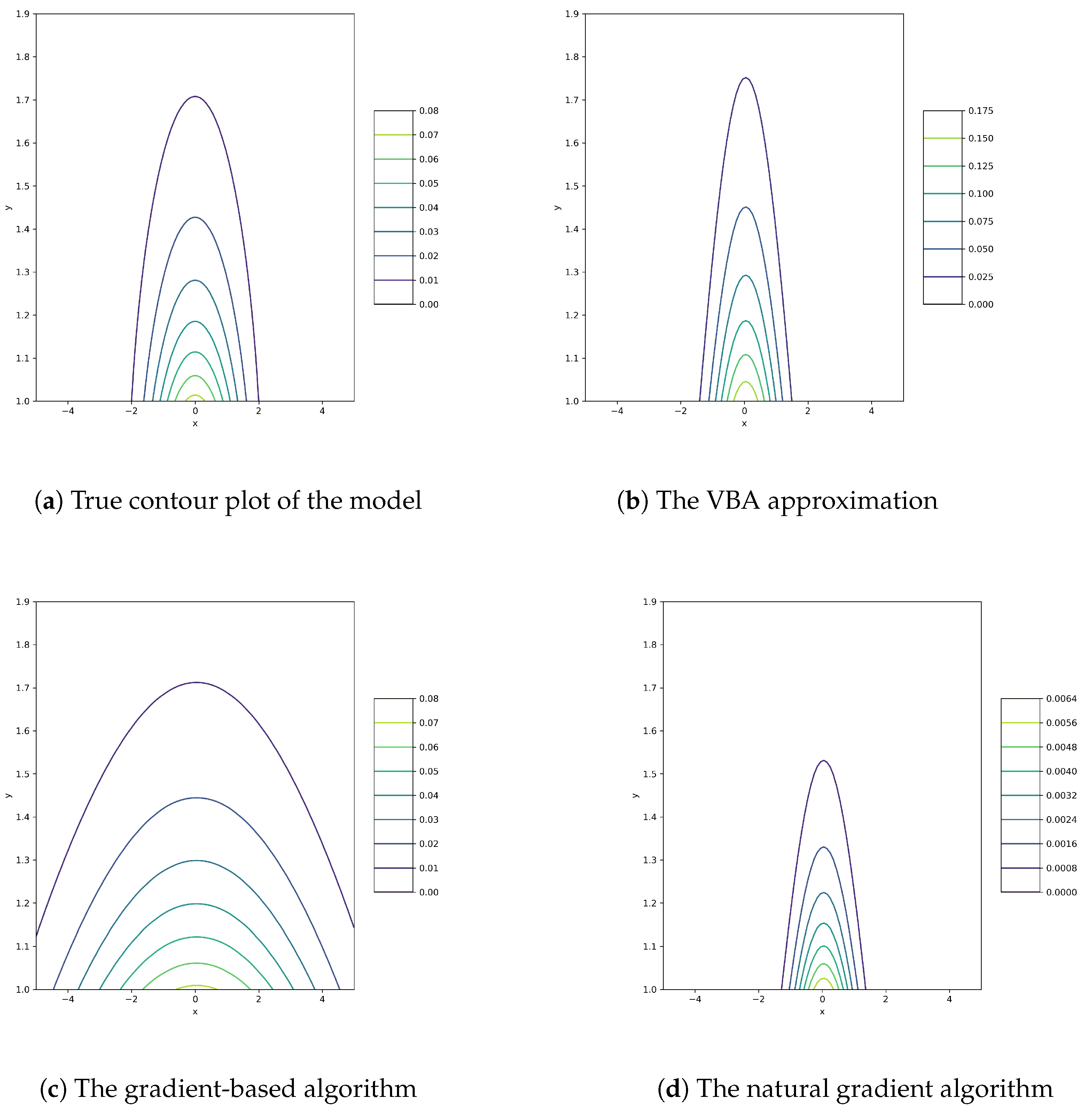
are the estimated parameters using, respectively, Algorithm 1, Algorithm 2 and Algorithm 3. The contour plots of the corresponding probability density functions are shown in
Figure 1 compared with original model.
All three algorithms try to minimize the same criterion. So, the objectives are all the same, but the number of steps may differ. The requirements must reach the minimum . In this simple example of the normal-inverse-gamma distribution, the convergence step numbers of VBA, gradient-based and natural gradient are 1, 2 and 1 using moment initializations. The overall performance of the standard alternate optimization (VBA) is more precise than any other. The poorest estimation is from a gradient-based algorithm. So, the algorithms are able to approximate the joint density function with a separable one but with different accuracy. In the following section, we will tackle a more complex model.
5. Multivariate Normal-Inverse-Wishart Example
In previous section, we explained how to preform VBA in order to approximate a complicated joint distribution function by tractable marginal factorials using a simple case study. In this section, a multivariate normal case is considered, which is approximated by for different shapes of the covariance matrix .
We assume that the basic structure of an available dataset is multivariate normal with unknown mean vector
and variance–covariance matrix
. Their joint prior distribution is a normal-inverse-Wishart distribution of
, which is the generalized form of the classical
. The posteriors are multivariate normal for mean vector and inverse-Wishart in the variance–covariance matrix. Since the normal-inverse-Wishart distribution is a conjugate prior distribution for multivariate normal, the posterior distribution of
and
again belongs to the same family, and their corresponding margins are
where
n is the sample size. To present the performance of the three algorithms, we examined on a dataset based on
, whose parameters have the following low-density structure:
We used only the data of
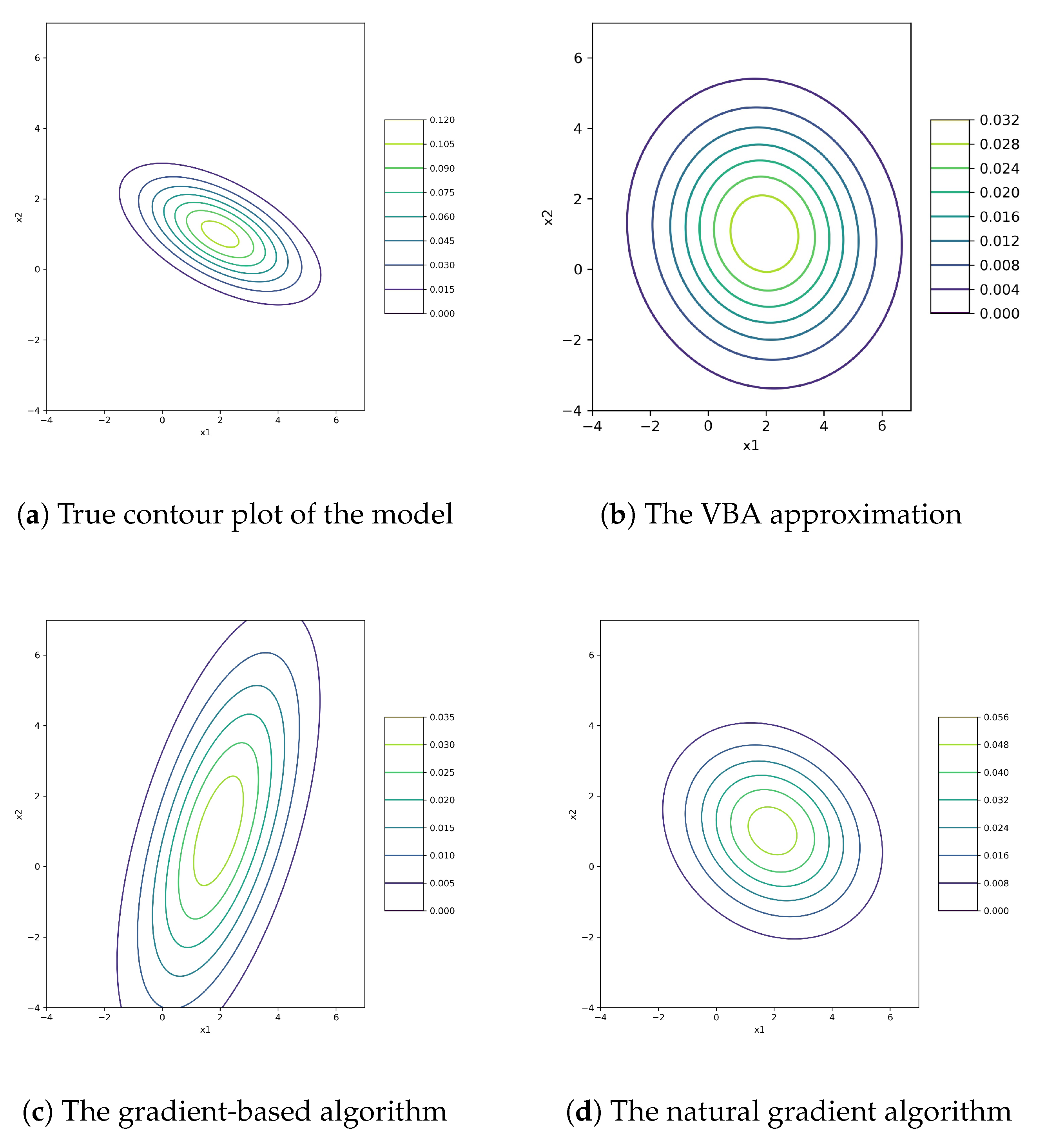
in the estimation processes. The results of algorithms are presented in
Figure 2 along with the true contour plot of the model. The VBA estimation is the most separable distribution compared with gradient and natural gradient methods. The next best case is the natural gradient algorithm, but its weakness is transferring the dependency slightly to the approximation. The results for the gradient-based algorithm show the dependency completely, along with its inability to obtain a separable model.
6. Simple Linear Inverse Problem
Finally the third example is the case of linear inverse problems with
with priors
,
and
, where
and
. Using these priors, we get
with
. See [
13] for details.
Thus, the joint distribution of
,
, and
:
is approximated by
using the VBA method. Even if the main interest is the estimation of
, but in the recursive process,
and
are also updated. For simplicity, we suppose that the transfer matrix
is an identical matrix
. The final outputs are as follows:
For simulations, we chose a model to examine the performance of these margins and compare them with gradient and natural gradient algorithms. The selected model is
with the following assumptions:
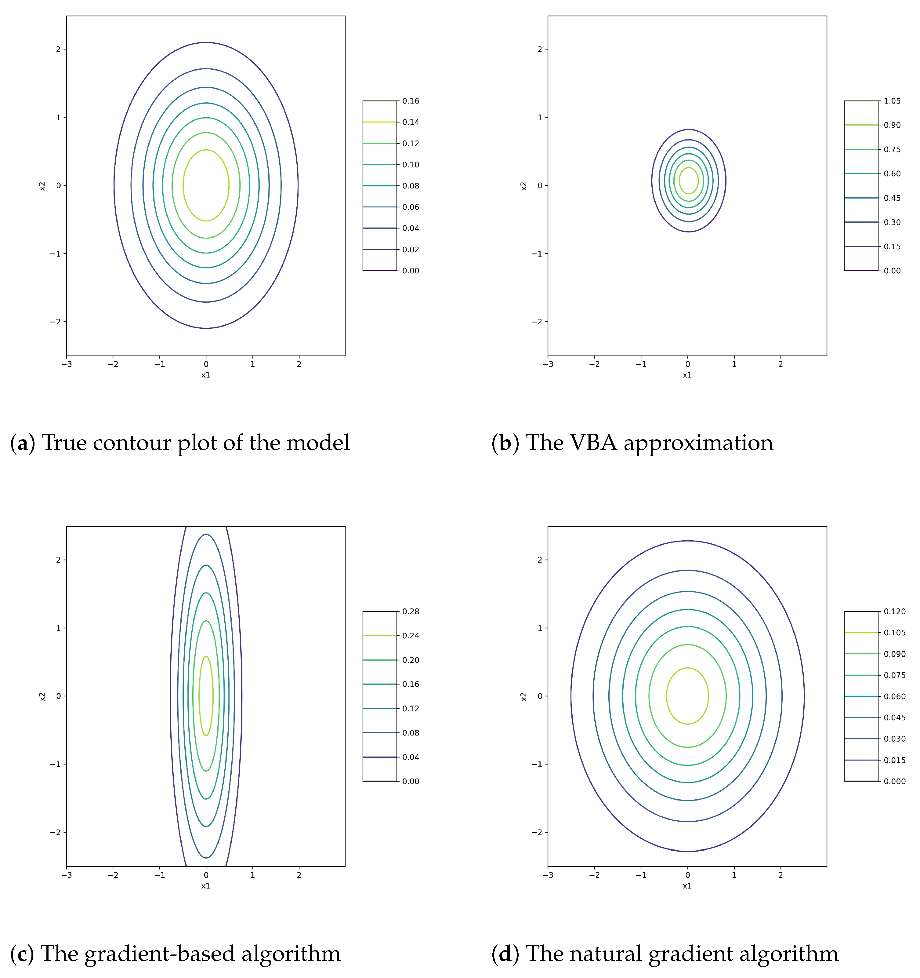
In the assessment procedure, we do not apply the above information. The output of algorithms are shown in
Figure 3, as well as the actual contour plot. In this example, the best diagnosis is from the natural gradient algorithm. The VBA by construction is separable and cannot be the same as the original.
7. Conclusions
This paper presents an approximation method of the unknown density functions for hidden variables called VBA. It is compared with gradient and natural gradient algorithms. We also consider three examples normal-inverse-gamma, normal-inverse-Wishart and linear inverse problem. We provided details of the first model and showed examples of two other examples throughout the whole paper. In all three models, the parameters are unexplored and need to be estimated by recursive algorithms. We attempted to approximate the joint complex distribution with a simpler version of the margin factorials that appeared to be independent cases. The VBA and natural gradient converged fairly early. The major discrepancy in algorithms comes from the accuracy of the results. They estimate the intricate joint distribution with separable ones. Here, the best overall performance of VBA is demonstrated.


