The Geometry of Quivers ^†

Abstract

Quivers are oriented graphs that have profound connections to various areas of mathematics, including representation theory and geometry. Quiver representations correspond to a vast generalization of classical linear algebra problems. The geometry of these representations can be described in the framework of Hamiltonian reduction and geometric invariant theory, giving rise to the concept of quiver variety. In parallel to these developments, quivers have appeared to naturally encode certain supersymmetric quantum field theories. The associated quiver variety then corresponds to a part of the moduli space of vacua of the theory. However, physics tells us that another natural geometric object associated with quivers exists, which can be seen as a magnetic analog of the (electric) quiver variety. When viewed from that angle, magnetic quivers are a new tool, developed in the past decade, that help mathematicians and physicists alike to understand geometric spaces. This note is the writeup of a talk in which I review these developments from both the mathematical and physical perspective, emphasizing the dialogue between the two communities.

1. A First Look at Quivers

This note is intended as an appetizer to the beautiful theory of quivers and certain geometric spaces associated with supersymmetric field theories. We mostly focus on examples, referring to the cited articles for the general theory. Section 1 provides an overview of the theory of quiver representations, based on the pedagogical references [1,2]. The main goal is to introduce Nakajima quiver varieties. Section 2 shows how these varieties appear as branches of vacua in certain supersymmetric theories. Section 3 introduces another variety associated with a quiver and defines the notion of magnetic quiver.

1.1. Quiver Representations

A quiver is a finite directed graph: it contains a finite set of vertices I and a finite set of arrows $\Omega \subseteq I^2$. A quiver, very much like a group, is an abstract structure that gains flesh when it is represented. We will focus here on linear representations of a quiver $\overrightarrow{Q}$. A linear representation of $\overrightarrow{Q}$ is a collection of finite-dimensional vector spaces $V_i$, one for each vertex $i\in I$, together with linear maps $V_i\to V_j$ for each $(i,j)\in \Omega$. For concreteness, one can pick $V_i={\mathbb{C}}^{v_i}$ (the vector $\mathbf{v}$ is then called the dimension of the representation), and the linear maps are chosen in the space

$$R(\overrightarrow{Q},\mathbf{v})=\underset{(i,j)\in \Omega }{⨁}\mathrm{Hom}({\mathbb{C}}^{v_i},{\mathbb{C}}^{v_j}).$$

(1)

The group $\mathrm{PGL}\left(\mathbf{v}\right)=\left(\prod \mathrm{GL}(v_i,\mathbb{C})\right)/{\mathbb{C}}^{*}$ acts on the representation space $R(\overrightarrow{Q},\mathbf{v})$ by conjugation and corresponds to the arbitrariness in the choice of bases in the spaces $V_i$ that allow one to represent the linear maps via matrices. The set of isomorphism classes of representations of dimension $\mathbf{v}$ can be identified with the quotient $R(\overrightarrow{Q},\mathbf{v})/\mathrm{PGL}\left(\mathbf{v}\right)$, which is the set of $\mathrm{PGL}\left(\mathbf{v}\right)$-orbits in $R(\overrightarrow{Q},\mathbf{v})$:

$$\left\{\begin{array}{c}\mathrm{Isomorphism}\mathrm{classes}\mathrm{of}\\ \mathbf{v}-\dim \mathrm{representations}\end{array}\right\}\leftrightarrow \left\{\begin{array}{c}\mathrm{GL}\left(\mathbf{v}\right)-\mathrm{orbits}\\ \mathrm{in}R(\overrightarrow{Q},\mathbf{v})\end{array}\right\}\leftrightarrow R(\overrightarrow{Q},\mathbf{v})/\mathrm{PGL}\left(\mathbf{v}\right)$$

(2)

We will come back to some of the problems that this naive definition poses. Before that, let us look at a few examples.

1.2. Examples and Basic Notions

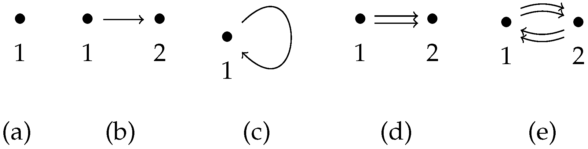
Figure 1 shows five examples of quivers. Let us look at their representations. Along the way, we introduce certain essential notions. For any quiver $\overrightarrow{Q}$, a representation is called simple if it contains no nontrivial subrepresentations; it is called semisimple if it is (isomorphic to) a direct sum of simple representations.

Example 1.

Let us start with the simplest quiver, with one vertex and no arrow, see Figure 1a. An n-dimensional representation of this quiver is simply an n-dimensional vector space, which is the direct sum of n copies of the one-dimensional representation $\mathbb{C}$. This one-dimensional representation is the building block of all others: it is simple, while the direct sums are semisimple.

For a quiver $\overrightarrow{Q}$, each orbit $\mathcal{O}$ is a nonsingular algebraic variety whose closure is $\overline{\mathcal{O}}=\mathcal{O}\cup X$ where X is a union of orbits of lower dimension. In addition, $\overline{\mathcal{O}}$ contains a unique closed orbit. If $\mathcal{O}$ is the orbit of a representation V, that closed orbit corresponds to a semisimple representation, which is called the semisimplification$V^{\mathrm{ss}}$ of V. The set of closed orbits coincides with the set of isomorphic classes of semisimple representations:

$$\left\{\begin{array}{c}\mathrm{Isomorphism}\mathrm{classes}\mathrm{of}\\ \mathrm{semisimple}\mathbf{v}-\dim \mathrm{representations}\end{array}\right\}\leftrightarrow \left\{\begin{array}{c}\mathrm{Closed}\mathrm{GL}\left(\mathbf{v}\right)\\ -\mathrm{orbits}\mathrm{in}R(\overrightarrow{Q},\mathbf{v})\end{array}\right\}\leftrightarrow R(\overrightarrow{Q},\mathbf{v})⫽\mathrm{PGL}\left(\mathbf{v}\right)$$

(3)

What appears on the right is the GIT (geometric invariant theory) quotient [3]: if M is a complex affine variety and G is a reductive group acting algebraically on M, $M⫽G$ is by definition the spectrum of the ring of invariants $\mathbb{C}{\left[M\right]}^G$. As a topological space, it is identified with the set of closed G-orbits in M, and there is a surjection $M/G\to M⫽G$, which associates each orbit $\mathcal{O}$ with the unique closed orbit contained in $\overline{\mathcal{O}}$.

Example 2.

For the quiver Figure 1b, a representation of dimension $\mathbf{v}=(v_1,v_2)$ is a pair of vector spaces of dimensions $v_1$ and $v_2$ together with a linear map between them. Equivalently, it is a $v_2\times v_1$ matrix. The group $\mathrm{GL}\left(\mathbf{v}\right)=\mathrm{GL}\left(v_1\right)\times \mathrm{GL}\left(v_2\right)$ acts by left-right multiplication on that matrix. This is the classical problem of equivalence of matrices (not to be confused with similarity, see the next example). It is well-known that the orbits correspond to the sets ${\mathcal{O}}_r$ of matrices of fixed rank $r\in \{0,1,\cdots ,r_{\max }=\min (v_1,v_2)\}$. Therefore, $R(\overrightarrow{Q},\mathbf{v})/\mathrm{PGL}\left(\mathbf{v}\right)$ contains $1+\min (v_1,v_2)$ points $\{{\mathcal{O}}_0,{\mathcal{O}}_1,\cdots ,{\mathcal{O}}_{r_{\max }}\}$. It is clear that ${\mathcal{O}}_r$ for $r>0$ is Zariski open, and its closure is the set of matrices of rank $\le r$, which is the union

$$\overline{{\mathcal{O}}_r}={\mathcal{O}}_0\cup {\mathcal{O}}_1\cup \cdots \cup {\mathcal{O}}_r.$$

(4)

On the other hand, ${\mathcal{O}}_0$ is (obviously) the unique closed orbit. The closure of every orbit ${\mathcal{O}}_r$, $r\ge 0$ contains a unique closed orbit ${\mathcal{O}}_0$. We formulate this fact geometrically by saying that $R(\overrightarrow{Q},v)⫽\mathrm{PGL}\left(v\right)$ is a point.

Example 3.

The quiver in Figure 1c is the Jordan quiver. Classifying its representations is the fundamental problem of linear algebra, which consists of classifying $v\times v$ matrices (or endomorphisms) up to similarity—the orbits are conjugacy classes. The full solution over $\mathbb{C}$ is given by the Jordan form, and the closed orbits correspond to diagonalizable matrices. Geometrically, this means that while $R(\overrightarrow{Q},v)/\mathrm{PGL}\left(v\right)$ has a complicated structure,

$$R(\overrightarrow{Q},v)⫽\mathrm{PGL}\left(v\right)=\mathrm{Spec}\left(\mathbb{C}{[{\lambda }_1,\cdots ,{\lambda }_v]}^{S_v}\right)={\mathbb{C}}^v/S_v.$$

(5)

The lesson from the last two examples generalizes: the quiver needs to have oriented cycles for $R(\overrightarrow{Q},v)⫽\mathrm{PGL}\left(v\right)$ not to be reduced to a point. A particularly interesting class of quivers having oriented cycles are double quivers, introduced next.

1.3. Double Quivers

Double quivers are quivers $Q^{\#}$ such that arrows can be partitioned into pairs $(H_{i,j},{\overline{H}}_{i,j})$ where if H connects vertex i to j, then $\overline{H}$ connects j to i, for $(i,j)\in \Omega$—see Figure 1e for an example. If we call $\overrightarrow{Q}$ the quiver obtained by deleting the $\overline{H}$ arrows, it is straightforward to see that $R(Q^{\#},\mathbf{v})=T^{*}R(\overrightarrow{Q},\mathbf{v})$. This is a symplectic space with a Hamiltonian action of $\mathrm{GL}\left(\mathbf{v}\right)$, with the moment map being given by

$${\mu }_{(Q^{\#},\Omega ,\mathbf{v})}:R(Q^{\#},\mathbf{v})\to \mathfrak{gl}\left(\mathbf{v}\right),{\mu }_{(Q^{\#},\Omega ,\mathbf{v})}\left(\left\{(H_{i,j},{\overline{H}}_{i,j})\right\}\right)=\sum _{(i,j)\in \Omega }[H_{i,j},{\overline{H}}_{i,j}].$$

(6)

Because of the numerous loops, the space $R(Q^{\#},\mathbf{v})⫽\mathrm{PGL}\left(\mathbf{v}\right)$ is complicated, and intuitively it is not a natural object to consider as it loses its symplectic structure (this is obvious, e.g., if the dimension of $\mathrm{PGL}\left(\mathbf{v}\right)$ is odd). It is more natural to consider the Hamiltonian reduction${\mu }^{-1}\left(0\right)⫽\mathrm{PGL}\left(v\right)$. The intuition behind this comes from the situation where M is a smooth symplectic manifold of real dimension n with a free proper Hamiltonian action of a real Lie group G of dimension d with moment map $\mu$. In this case, $T^{*}(M/G)$ is symplectomorphic to ${\mu }^{-1}\left(0\right)/G$. The real dimension is $2n-d-d$, where the first $-d$ comes from the $\mu$-level set, and the second one comes from the quotient. The construction of ${\mu }^{-1}\left(0\right)⫽\mathrm{PGL}\left(v\right)$ is the algebraic analog, and it allows for singularities and fixed points under the group action.

1.4. Quiver Varieties

We are now ready for the central character of this note. The notion of quiver variety is usually defined based on the notion of framed quiver representation. Here, we follow a slightly different but totally equivalent route—the equivalence being what is sometimes called the Crawley–Boevey trick [4]. We fix a graph Q (with set of vertices I and a set of unoriented edges $\Omega \subseteq S^2\left(I\right)$; for simplicity, we assume there are no edges connecting a vertex to itself) and a dimension vector $\mathbf{v}$ such that at least one entry of $\mathbf{v}$ is equal to 1: $v_{i_0}=1$. We call $\widehat{\mathbf{v}}$ the vector $\mathbf{v}$ with that entry removed. The corresponding Nakajima quiver variety ${\mathcal{M}}_H(Q,\mathbf{v})$ is then by definition [5,6]

$${\mathcal{M}}_H(Q,\mathbf{v})={\widehat{\mu }}^{-1}\left(0\right)⫽\mathrm{GL}\left(\widehat{\mathbf{v}}\right),$$

(7)

where $\widehat{\mu }$ is the projection of the moment map $\mu$ of the corresponding double quiver $Q^{\#}$ onto the Lie algebra $\mathfrak{gl}\left(\widehat{\mathbf{v}}\right)$. Intuitively, this means that we impose the vanishing of the commutators (6) only at vertices $i\ne i_0$, and we impose invariance only with respect to the $\mathrm{GL}\left(v_i\right)$ for $i\ne i_0$. Importantly, this definition does not depend on the choice of $i_0$.

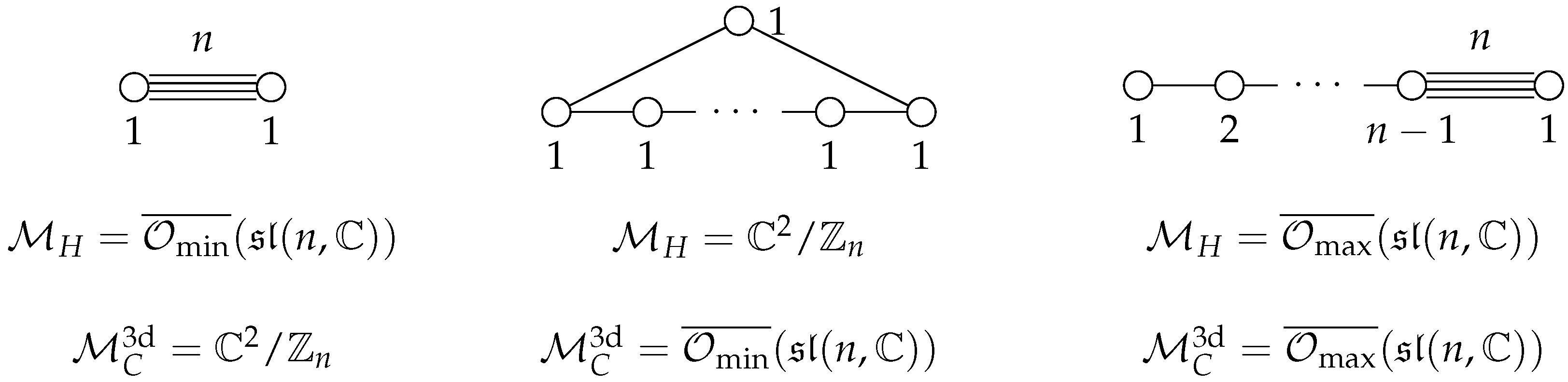
Examples of quivers are shown in Figure 2—the quivers are entirely specified by the underlying graph, and by convention the graphs themselves are also called quivers. It is a good exercise for the reader to derive the varieties ${\mathcal{M}}_H$ for these three fundamental examples. We deal in detail only with the first one here. We pick the left node for $i_0$. Therefore, the n edges give rise in the double quiver to $2n$ arrows that one can group into two maps $H\in \mathrm{Hom}(\mathbb{C},{\mathbb{C}}^n)$ and $\overline{H}\in \mathrm{Hom}({\mathbb{C}}^n,\mathbb{C})$. The moment map $\widehat{mu}$ reduces to $H\overline{H}$, and $\mathrm{GL}\left(\widehat{\mathbf{v}}\right)={\mathbb{C}}^{*}$ acts on $(H,\overline{H})$ with charge $(+1,-1)$. One then checks that

$$\begin{array}{ccc}\hfill {\mathcal{M}}_H(Q,\mathbf{v})& =& \{(H,\overline{H})\in \mathrm{Hom}(\mathbb{C},{\mathbb{C}}^n)\times \mathrm{Hom}({\mathbb{C}}^n,\mathbb{C})|H\overline{H}=0\}⫽{\mathbb{C}}^{*}\hfill \\ & =& \{M\in \mathrm{Hom}({\mathbb{C}}^n,{\mathbb{C}}^n)|M^2=0,\mathrm{rank}\left(M\right)\le 1,\mathrm{tr}\left(M\right)=0\},\hfill \end{array}$$

(8)

the equality being given by $M=\overline{H}H$. This is the closure of the minimal nilpotent orbit of $\mathfrak{sl}(n,\mathbb{C})$. In a similar way, one can show that the quiver varieties for the second and third quivers are, respectively, the Klein singularities ${\mathbb{C}}^2/{\mathbb{Z}}_n$ (the complex hypersurface $x^2+y^2+z^n=0$ in ${\mathbb{C}}^3$), also called $A_{n-1}$, and the closure of the maximal nilpotent orbit in $\mathfrak{sl}(n,\mathbb{C})$.

2. The Electric Side

2.1. Physical Theories and Quivers

In this section, we lay down some fundamental materials in supersymmetric quantaum field theory, and we find a natural connection with the notions in the previous section. The standard model of particle physics is the quantaum field theory (QFT) that best describes our world and its elementary constituents. The building blocks with high energy are as follows (we leave aside the Higgs field (which is a scalar field) as it plays no significant role in this presentation, and its special status disappears once we consider the supersymmetric models below ):

• A gauge group, which encodes the fundamental forces (electromagnetism, weak and strong forces). This is a Lie group whose complexified Lie algebra is ${\mathfrak{g}}_{\mathrm{SM}}={\mathfrak{sl}}_3\oplus {\mathfrak{sl}}_2\oplus {\mathfrak{gl}}_1$. The forces are mediated by massless gauge bosons$A_{\mu }$, which are vector fields valued in the adjoint representation of that algebra.
• Matter constituents, which are fermion fields $\psi$ valued in bifundamental (a bifundamental representation of a semisimple Lie algebra $\mathfrak{g}$ is the product of a fundamental representation of a simple summand of $\mathfrak{g}$ with the antifundamental representation of a summand of $\mathfrak{g}$.) representations of ${\mathfrak{g}}_{\mathrm{SM}}$. This matter content can be encoded in a quiver where the vertices are the simple summands of ${\mathfrak{g}}_{\mathrm{SM}}$ and the arrows are the matter fields.

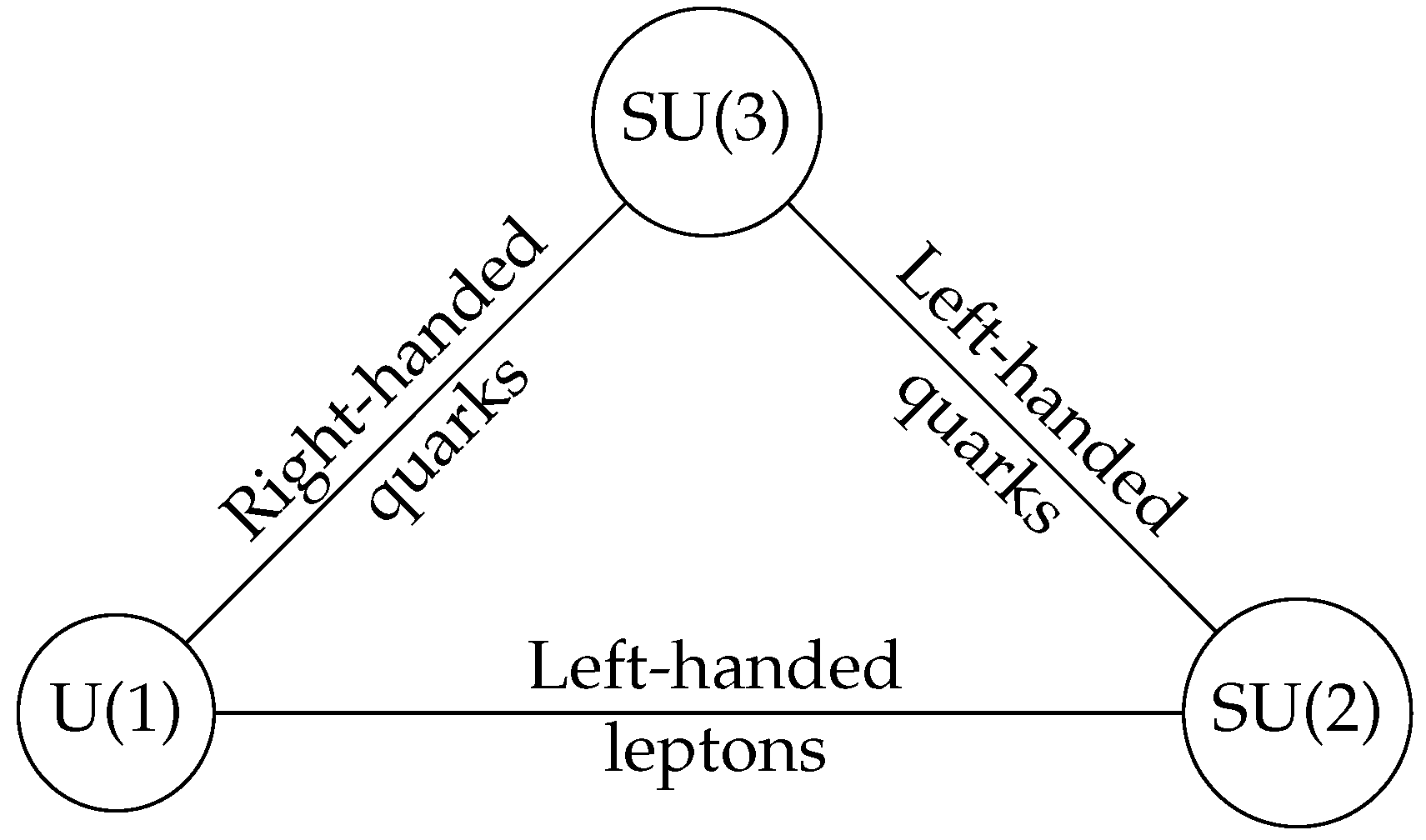
A very schematic depiction of the standard model is shown in Figure 3. In addition to these data, one should also specify the masses of the matter fields and various interaction terms to fully define the theory. The situation is different when supersymmetry enters the stage.

2.2. Supersymmetric Quiver Gauge Theories

Centuries of observations of Nature by physicists have lead to the observation that the fundamental laws are invariant under translation in space and time (with generators $P_{\mu }$), rotations in space, and boosts of special relativity (together, these are described by generators $M_{\mu \nu }$). These transformations together form the Poincaré group, which can be studied locally via its Lie algebra, the ten-dimensional Poincaré algebra, with generators $P_{\mu }$ and $M_{\mu \nu }$. Essentially, one kind of extension of that algebra exists that is consistent with the fundamental principles of quantum mechanics: supersymmetry. It consists of adding supercharges, which are fermionic generators $Q^I$ and ${\overline{Q}}^I$, for $I=1,\cdots ,\mathcal{N}$. These can be thought of as square roots of translations, as (here, $Q^I$ are left-handed Weyl spinors, ${\overline{Q}}^J$ are right-handed, $\{·,·\}$ is the anticommutator, and ${\sigma }^{\mu }=({\mathbf{1}}_2,{\sigma }^i)$ where the ${\sigma }^i$ are the Pauli matrices) $\{Q^I,{\overline{Q}}^J\}=2P_{\mu }{\sigma }^{\mu }{\delta }^{IJ}$. With each generator being a spinor, there are actually $4\mathcal{N}$ supercharges in the theory.

In a supersymmetric theory, the supercharges $Q^I$ relate fields with different statistics (bosons and fermions). When $\mathcal{N}=1$, there is essentially one fermionic superpartner for each boson; conversely, their spins differ by $\frac{1}{2}$.

We consider the case $\mathcal{N}=2$ (i.e., 8 supercharges) throughout this note, and we generalize the construction of the standard model above by taking a gauge algebra $\mathfrak{g}={\mathfrak{gl}}_{n_1}\oplus \cdots {\mathfrak{gl}}_{n_r}$, and massless matter fields transforming in various bifundamental representations. This can be encoded into a graph Q, with the simple summands of $\mathfrak{g}$ as vertices and matter fields as edges. A fundamental consequence of supersymmetry is that once the graph Q is given, one needs only to supplement it with the gauge couplings (one real number per node) to fully specify the theory. Regarding the building blocks listed in Section 2.1, we also need to know that:

• The gauge bosons are part of vector multiplets, which contain spin $\frac{1}{2}$ gauginos and one complex scalar field $\varphi$ in the adjoint representation of the gauge algebra.
• The matter fermions are part of hypermultiplets, which contain a pair of complex scalar fields $(H,\overline{H})$ that transforms in a representation of the form $R\oplus \overline{R}$ of the gauge algebra.

When confronted with a QFT, the first question to ask is about the vacuum, around which one can then use perturbation theory (represented pictorially by Feynman diagrams). In theories with large amounts of symmetry, there can be several degenerate vacua, and in fact in the present case there are infinitely many. The emphasis on scalar fields above is due to the following observation: they are the only fields that can take a non-zero value in the vacua without breaking Poincaré invariance. Because of sypersymmetry, the space of vacua turns out to be an algebraic variety $\mathcal{M}$, called the vacuum moduli space, parametrized by the gauge invariant combinations of scalar fields ϕ and $(H,\overline{H})$. The part that is parametrized by $(H,\overline{H})$ only is called the Higgs branch, denoted ${\mathcal{M}}_H$, while the part that is parametrized by $\varphi$ only is called the Coulomb branch, denoted ${\mathcal{M}}_C^{4\mathrm{d}}$ (the reason for the superscript will become clear in Section 3).

2.3. Higgs Branches, Quiver Varieties, and Beyond

In this section, we focus on the Higgs branch ${\mathcal{M}}_H$. The structure of the hypermultiplets shows that a configuration of VEVs for $(H,\overline{H})$ corresponds to a representation of the double quiver $Q^{\#}$ with a dimension given by the gauge algebra $\mathfrak{g}$. Due to supersymmetry, the vacuum equations take the form of the vanishing of the moment map (6), while the requirement of gauge invariance is reflected mathematically in the GIT quotient in (7). Therefore, the Higgs branch is identified with the quiver variety discussed in Section 1.4.

The Higgs branch ${\mathcal{M}}_H$ of a 4d $\mathcal{N}=2$ quiver gauge theory whose gauge group is a product of unitary groups $\mathrm{U}\left(v_i\right)$ is therefore specified by a graph Q and a dimension vector $\mathbf{v}$, which satisfy the constraints listed in Section 1.4. A straightforward but vast generalization is obtained by considering different types of gauge groups: $\mathrm{SU}\left(v_i\right)$, $\mathrm{Sp}\left(v_i\right)$, and $\mathrm{SO}\left(v_i\right)$, but also discrete groups or mixtures thereof. It is also known that certain QFTs with $\mathcal{N}=2$ supersymmetry can be defined that cannot be described using the vector multiplets and hypermultiplets as above; however, the notion of the Higgs branch is still well defined. This is the case for some of the so-called class S theories, built from compactifying a six-dimensional theory on a Riemann surface [7], or for the Argyres–Douglas theories [8].

In all cases, ${\mathcal{M}}_H$ is a singular complex variety that admits a stratification into symplectic leaves. One prototypical example is shown in Figure 4: the nilpotent cone of $\mathfrak{sl}(4,\mathbb{C})$ is stratified by the various nilpotent orbits. Physically, for the gauge theories this stratification represents the different phases, which differ by how broken the gauge group is in a given vacuum; the mechanism of partially breaking the gauge invariance using the vacuum expectation value of scalar fields is well known in particle physics as the Higgs mechanism—hence the name of that branch. It is, in general, challenging to compute this stratification. In the next section, we use physical insight to present a partial solution to that problem.

3. The Magnetic Side

3.1. Three-Dimensional Coulomb Branches and Magnetic Quivers

At the end of Section 2.2, we have introduced the Coulomb branch ${\mathcal{M}}_C^{4\mathrm{d}}$. The geometry of ${\mathcal{M}}_C^{4\mathrm{d}}$ is quite different from that of ${\mathcal{M}}_H$, while ${\mathcal{M}}_H$ is a singular version of a hyperKähler manifold—a symplectic singularity [9], ${\mathcal{M}}_C^{4\mathrm{d}}$ is a singular version of a so-called special Kähler manifold [10]. However, the two structures are close enough: the cotangent bundle of a special Kähler manifold carries a hyperKähler structure [11]. One way this can be realized physically is to compactify the 4d theory on a small circle, i.e., placing the theory on ${\mathbb{R}}^{1,2}\times S^1$ and letting the inverse radius $1/R$ of $S^1$ be large compared to the observation energy scale. In this way, one reaches a 3d theory whose Coulomb branch ${\mathcal{M}}_C^{3\mathrm{d}}$, defined analogously as in 4d, is a symplectic singularity. The Higgs branch of that 3d theory is identical to the Higgs branch of the 4d theory, so no superscript is needed there. Using this process, we have defined for any graph Q and good vector $\mathbf{v}$ a symplectic singularity ${\mathcal{M}}_C^{3\mathrm{d}}(Q,\mathbf{v})$. The precise mathematical definition of that space has been constructed in [12,13] based on the expectations from physics [14,15,16].

While the Higgs branch is parametrized by fields that carry a kind of electric charge under the various gauge groups, the 3d Coulomb branch is paramatrized by gauge field configuration that corresponds to magnetic monopoles [17,18]. This explains the terminology according to which ${\mathcal{M}}_H$ is the electric side of the moduli space while ${\mathcal{M}}_C$ is its magnetic side.

We now turn to the other crucial notion of this short note. Given a symplectic singularity S, we say that $(Q,\mathbf{v})$ is a magnetic quiver for S if $S={\mathcal{M}}_C^{3\mathrm{d}}(Q,\mathbf{v})$. It turns out there is a conjectured algorithm, called quiver subtraction [19,20,21,22], that provides the singularity structure of S if a magnetic quiver $(Q,\mathbf{v})$ is known. The evidence for the correctness of this algorithm relies on various dualities in string theory. As an illustration, we apply this algorithm to the nilpotent cone of $\mathfrak{sl}(n,\mathbb{C})$ given as in Figure 2, recovering the usual stratification into nilpotent orbits. An illustration for $n=4$ is shown in Figure 4.

The simplest incarnation of the concept of magnetic quiver is the so-called 3d mirror symmetry [23] for unitary quivers. When two theories defined by $(Q_1,{\mathbf{v}}_1)$ and $(Q_2,{\mathbf{v}}_2)$ are a 3d mirror, we have

$${\mathcal{M}}_H(Q_1,{\mathbf{v}}_1)={\mathcal{M}}_C^{3\mathrm{d}}(Q_2,{\mathbf{v}}_2)\mathrm{and}{\mathcal{M}}_C^{3\mathrm{d}}(Q_1,{\mathbf{v}}_1)={\mathcal{M}}_H(Q_2,{\mathbf{v}}_2).$$

(9)

The two leftmost quivers in Figure 2 form such a mirror pair, while the rightmost quiver represents a self-mirror theory. A natural question, when confronted with a mirror pair, is the relation between the Higgs branches of both theories. It is conjectured that this coincides with the notion of symplectic duality put forward in [24].

3.2. The Scope of Magnetic Quivers

The definition of magnetic quiver given in the previous paragraph does not require S to be the Higgs branch of a quiver gauge theory; the notion is more general and can be applied in an abstract mathematical setting (see, e.g., [25,26,27] for the use of magnetic quivers in the context of hyperKähler implosion spaces).

Conversely, even within the realm of Higgs branches one can go much beyond Nakajima quiver varieties, as we saw in Section 2.3. It turns out one can often still find magnetic quivers for these Higgs branches [28,29,30,31,32,33,34], thus opening a window into the geometry of the moduli space, and various deductions about deformations and the renormalization group flow. Another subtlety arises when the Higgs branch is not an irreducible variety. In that case, it might be necessary to provide several magnetic quivers, along with quivers for the intersections of the irreducible varieties.

The consequences of the two spaces, Higgs and Coulomb, that can be associated with quivers are still to be fully understood and are the subject of intense investigation.

References

- Ginzburg, V. Lectures on Nakajima’s quiver varieties. arXiv 2009, arXiv:0905.0686. [Google Scholar]
- Kirillov, A., Jr. Quiver Representations and Quiver Varieties; American Mathematical Soc.: Providence, RI, USA, 2016; Volume 174. [Google Scholar]
- Mumford, D.; Fogarty, J.; Kirwan, F. Geometric Invariant Theory; Springer Science & Business Media: Berlin, Germany, 1994; Volume 34. [Google Scholar]
- Crawley-Boevey, W. Geometry of the moment map for representations of quivers. Compos. Math. 2001, 126, 257–293. [Google Scholar] [CrossRef]
- Nakajima, H. Instantons on ALE spaces, quiver varieties, and Kac-Moody algebras. Duke Math. J. 1994, 76, 365–416. [Google Scholar] [CrossRef]
- Nakajima, H. Quiver varieties and Kac-Moody algebras. Duke Math. J. 1998, 91, 515–560. [Google Scholar] [CrossRef]
- Gaiotto, D. N = 2 dualities. JHEP 2012, 8, 034. [Google Scholar] [CrossRef]
- Argyres, P.C.; Douglas, M.R. New phenomena in SU(3) supersymmetric gauge theory. Nucl. Phys. B 1995, 448, 93–126. [Google Scholar] [CrossRef]
- Beauville, A. Symplectic singularities. arXiv 1999, arXiv:math/9903070. [Google Scholar] [CrossRef]
- Freed, D.S. Special Kahler manifolds. Commun. Math. Phys. 1999, 203, 31–52. [Google Scholar] [CrossRef]
- Cecotti, S.; Ferrara, S.; Girardello, L. Geometry of Type II Superstrings and the Moduli of Superconformal Field Theories. Int. J. Mod. Phys. A 1989, 4, 2475. [Google Scholar] [CrossRef]
- Nakajima, H. Towards a mathematical definition of Coulomb branches of 3-dimensional N=4 gauge theories, I. Adv. Theor. Math. Phys. 2016, 20, 595–669. [Google Scholar] [CrossRef]
- Braverman, A.; Finkelberg, M.; Nakajima, H. Towards a mathematical definition of Coulomb branches of 3-dimensional N=4 gauge theories, II. Adv. Theor. Math. Phys. 2018, 22, 1071–1147. [Google Scholar] [CrossRef]
- Seiberg, N.; Witten, E. Gauge dynamics and compactification to three-dimensions. arXiv 1996, arXiv:hep-th/9607163. [Google Scholar]
- Cremonesi, S.; Hanany, A.; Zaffaroni, A. Monopole operators and Hilbert series of Coulomb branches of 3d N = 4 gauge theories. JHEP 2014, 1, 005. [Google Scholar] [CrossRef]
- Bullimore, M.; Dimofte, T.; Gaiotto, D. The Coulomb Branch of 3d N=4 Theories. Commun. Math. Phys. 2017, 354, 671–751. [Google Scholar] [CrossRef]
- Hooft, G. On the Phase Transition Towards Permanent Quark Confinement. Nucl. Phys. B 1978, 138, 1–25. [Google Scholar] [CrossRef]
- Borokhov, V.; Kapustin, A.; Wu, X.K. Topological disorder operators in three-dimensional conformal field theory. J. High Energy Phys. 2003, 2002, 049. [Google Scholar] [CrossRef]
- Cabrera, S.; Hanany, A. Quiver Subtractions. JHEP 2018, 9, 008. [Google Scholar] [CrossRef]
- Bourget, A.; Cabrera, S.; Grimminger, J.F.; Hanany, A.; Sperling, M.; Zajac, A.; Zhong, Z. The Higgs mechanism—Hasse diagrams for symplectic singularities. JHEP 2020, 1, 157. [Google Scholar] [CrossRef]
- Bourget, A.; Grimminger, J.F.; Hanany, A.; Sperling, M.; Zhong, Z. Branes, Quivers, and the Affine Grassmannian. arXiv 2021, arXiv:2102.06190. [Google Scholar]
- Bourget, A.; Grimminger, J.F.; Hanany, A.; Zhong, Z. The Hasse Diagram of the Moduli Space of Instantons. arXiv 2022, arXiv:2202.01218. [Google Scholar] [CrossRef]
- Intriligator, K.A.; Seiberg, N. Mirror symmetry in three-dimensional gauge theories. Phys. Lett. B 1996, 387, 513–519. [Google Scholar] [CrossRef]
- Braden, T.; Licata, A.; Proudfoot, N.; Webster, B. Quantizations of conical symplectic resolutions II: Category O and symplectic duality. Asterisque 2016, 384, 75–179. [Google Scholar]
- Dancer, A.; Hanany, A.; Kirwan, F. Symplectic duality and implosions. arXiv 2020, arXiv:2004.09620. [Google Scholar] [CrossRef]
- Bourget, A.; Dancer, A.; Grimminger, J.F.; Hanany, A.; Kirwan, F.; Zhong, Z. Orthosymplectic implosions. JHEP 2021, 8, 012. [Google Scholar] [CrossRef]
- Bourget, A.; Dancer, A.; Grimminger, J.F.; Hanany, A.; Zhong, Z. Partial Implosions and Quivers. J. High Energ. Phys. 2022. [Google Scholar] [CrossRef]
- Bourget, A.; Grimminger, J.F.; Hanany, A.; Sperling, M.; Zafrir, G.; Zhong, Z. Magnetic quivers for rank 1 theories. JHEP 2020, 9, 189. [Google Scholar] [CrossRef]
- Bourget, A.; Grimminger, J.F.; Martone, M.; Zafrir, G. Magnetic quivers for rank 2 theories. JHEP 2022, 3, 208. [Google Scholar] [CrossRef]
- Carta, F.; Giacomelli, S.; Mekareeya, N.; Mininno, A. Conformal manifolds and 3d mirrors of Argyres–Douglas theories. JHEP 2021, 8, 015. [Google Scholar] [CrossRef]
- Xie, D. 3D mirror for Argyres–Douglas theories. arXiv 2021, arXiv:2107.05258. [Google Scholar]
- Dey, A. Higgs Branches of Argyres–Douglas theories as Quiver Varieties. arXiv 2021, arXiv:2109.07493. [Google Scholar]
- Bourget, A.; Grimminger, J.F.; Hanany, A.; Kalveks, R.; Zhong, Z. Higgs branches of U/SU quivers via brane locking. JHEP 2022, 8, 061. [Google Scholar] [CrossRef]
- Bourget, A.; Grimminger, J.F. Fibrations and Hasse diagrams for 6d SCFTs. JHEP 2022, 12, 159. [Google Scholar] [CrossRef]
Figure 1.
Five examples of quivers. (a) Trivial quiver. (b) quiver. (c) Jordan quiver. (e) is the double of (d).
Figure 2.
Three graphs with the corresponding dimension vector , indicated as integers next to each node. Below each graph we write the Higgs and 3d Coulomb branches (see Section 3).
Figure 3.
A very schematic depiction of a portion of the matter content of the standard model of particle physics (right-handed leptons and the Higgs field are not represented). The nodes correspond to the gauge groups for the fundamental interactions (gauge bosons), and the edges correspond to matter fields (chiral fermions) charged under these forces. SU(3) is the strong force; SU(2) the weak isospin; and U(1) a combination of weak hypercharge and the baryonic charge, which makes the charge of the left-handed quarks vanish.
Figure 4.
Hasse diagram of nilpotent orbits of obtained via quiver subtraction, with the complex dimension of each leaf. The quivers at each step are shown on the right, while the pieces that are subtracted to move from one variety to its singular subvariety are drawn in red.
Disclaimer/Publisher’s Note: The statements, opinions and data contained in all publications are solely those of the individual author(s) and contributor(s) and not of MDPI and/or the editor(s). MDPI and/or the editor(s) disclaim responsibility for any injury to people or property resulting from any ideas, methods, instructions or products referred to in the content. |
© 2023 by the author. Licensee MDPI, Basel, Switzerland. This article is an open access article distributed under the terms and conditions of the Creative Commons Attribution (CC BY) license (https://creativecommons.org/licenses/by/4.0/).
Share and Cite
MDPI and ACS Style
Bourget, A. The Geometry of Quivers. Phys. Sci. Forum 2022, 5, 42. https://doi.org/10.3390/psf2022005042
AMA Style
Bourget A. The Geometry of Quivers. Physical Sciences Forum. 2022; 5(1):42. https://doi.org/10.3390/psf2022005042
Chicago/Turabian StyleBourget, Antoine. 2022. "The Geometry of Quivers" Physical Sciences Forum 5, no. 1: 42. https://doi.org/10.3390/psf2022005042
APA StyleBourget, A. (2022). The Geometry of Quivers. Physical Sciences Forum, 5(1), 42. https://doi.org/10.3390/psf2022005042