Outlier-Robust Surrogate Modelling of Ion-Solid Interaction Simulations ^†

Abstract

Data for complex plasma–wall interactions require long-running and expensive computer simulations of codes like EIRENE or SOLPS. Furthermore, the number of input parameters is large, which results in a low coverage of the (physical) parameter space. Unpredictable occasions of outliers create a need to conduct the exploration of this multi-dimensional space using robust analysis tools. We restate the Gaussian-process (GP) method as a Bayesian adaptive exploration method for establishing surrogate surfaces in the variables of interest. On this basis, we complete the analysis by the Student-t process (TP) method in order to improve the robustness of the result with respect to outliers. The most obvious difference between both methods shows up in the marginal likelihood for the hyperparameters of the covariance function where the TP method features a broader marginal probability distribution in the presence of outliers.

1. Introduction

Simulations of particles from fusion plasmas escaping confinement and interacting with the vessel wall are extremely costly in terms of computer power and time. Consequently, results from ion-solid interaction simulations, e.g., sputter rates from the software EIRENE/FZ Jülich [1], lack real time ability and fail to provide the fast numerical access needed, e.g., by gradient-based methods traveling through multi-dimensional parameter space while searching for extremal structures. With already acquired data as a starting basis, the method of surrogate modelling provides fast and easy access for numerical optimization methods. In the present case, the shape of utility functions used for the selection of the next optimal point [2] is relatively benign. In situations where this is not the case, the detrimental effect of spurious peaks in the utility function can partly be be avoided using modified acquisition strategies [3]. The EIRENE program employs at its heart a Monte Carlo method, by which it may be assumed to produce results with uncertainty margins that follow a Gaussian distribution. However, the code itself involves tables of source rates for particles, energies and momentum which may introduce some nonlinear behaviour at least to the variance of the results.

It has been known for a long time that a Student-t distribution offers the possibility of making the analysis more robust with respect to outliers [4,5]. In this paper, we follow this trail and investigate the Student-t process method as a surrogate surface emulator in competition with the Gaussian process method [6]. Introduced by Rasmussen et al. in Chapter 9.9 of his landmark publication “Gaussian Processes for Machine Learning” [6], the derivation and application of a Student-t process as a surrogate emulator was examined many times. Already, Yu et al. in 2007 [7] placed the TP-method on a solid foundation with correct data error handling, while Shah et al. [8] approached the same marginal likelihood by integrating an inverse Wishart process prior over the covariance kernel of the Gaussian Process.

In order to investigate the differences between the GP- and TP-method, we set up artificial test cases in one and two dimensions. The problem we want to tackle for the sputter rates caused by fusion plasmas takes place in a four-dimensional physics parameter set, so we have to transfer the results of the test cases derived with artificial data to analysis of real world data. As a side effect, the changes to the program for adaptation to the TP-method are validated by our well established algorithm emulating surrogate surfaces. Finally, we present results for fusion plasma sputter rates in a two-dimensional subspace of a four-dimensional parameter space.

2. Gaussian Process Method

The problem of predicting function values in a multi-dimensional space supported by given data is a regression problem for a non-trivial function of unknown shape. The matrix $\mathit{X}=({\mathit{x}}_1,{\mathit{x}}_2,\dots ,{\mathit{x}}_N)$ consisting of N input data vectors ${\mathit{x}}_i$ of dimension $N_{\dim }$ is given. The target data $\mathit{y}={(y_1,\dots y_N)}^T$ is blurred by Gaussian noise of variance ${\mathbf{\Delta }}_{ij}={{\sigma }_d}_i^2{\delta }_{ij}$. Quantity of interest is the target value $f_{*}$ at test input vector ${\mathit{x}}_{*}$ and is generated by a function $f\left(\mathit{x}\right)$ which shall satisfy $y=f\left(\mathit{x}\right)+ϵ$, with $\langle ϵ\rangle =0$ and $\langle {ϵ}^2\rangle ={\sigma }_d^2$. As a statistical process, it is fully defined by its covariance function, which is the place where we incorporate all the properties which we would like our (hidden) problem-describing function to have. For the functional form of the covariance we choose a Gaussian type exponent with the negative squared value of the distance between two input data vectors ${\mathit{x}}_p$ and ${\mathit{x}}_q$.

$$k({\mathit{x}}_p,{\mathit{x}}_q)={\sigma }_f^{2}exp\left\{-\frac{1}{2}{\left|\frac{{\mathit{x}}_p-{\mathit{x}}_q}{\lambda }\right|}^2\right\}.$$

(1)

The neighborhood of the two data vectors should be of relevance for the smoothness of the result, which is mimicked by a length scale $\lambda$ in the denominator to represent the long range dependence of the two vectors. Moreover, since the Gaussian process method defines a distribution over functions, the width of this distribution will have some influence on our result as well. This shall be comprised by the signal variance ${\sigma }_f^2$. The covariance of the input data is abbreviated as ${\mathit{K}}_{ij}=k({\mathit{x}}_i,{\mathit{x}}_j)$ and the vector of covariances between test input vector and a single input data is ${\left({\mathit{k}}_{*}\right)}_i=k({\mathit{x}}_{*},{\mathit{x}}_i)$. Finally, in addition to the above estimation of the variance of a distinct data point with ${\sigma }_{d_i}^2$, provided e.g., by the EIRENE MC-simulations, we consider an overall noise in the data by a variance ${\sigma }_n^2$. Starting with no further information about the hyperparameters, we assume Gaussian priors with $\mathcal{N}$(1,1).

Summing up the analysis from previous papers [6,9], the probability distribution for a single function value $f_{*}$ at test input $x_{*}$ is

$$p\left(f_{*}\right|\mathit{X},\mathit{y},{\mathit{x}}_{*})\propto \mathcal{N}\left({\overline{f}}_{*},\mathrm{var}\left(f_{*}\right)\right),$$

(2)

with mean

$${\overline{f}}_{*}={\mathit{k}}_{*}^T{\left(\mathit{K}+{\sigma }_n^2\mathbf{\Delta }\right)}^{-1}\mathit{y},$$

(3)

and variance

$${\mathrm{var}}^{\mathcal{GP}}\left(f_{*}\right)=\mathit{k}({\mathit{x}}_{*},{\mathit{x}}_{*})-{\mathit{k}}_{*}^T{\left(\mathit{K}+{\sigma }_n^2\mathbf{\Delta }\right)}^{-1}{\mathit{k}}_{*}.$$

(4)

The hyperparameters ${\mathbf{\theta }}^T=(\lambda ,{\sigma }_f,{\sigma }_n)$ determine the result of the Gaussian process method. Since we do not know a priori which setting is useful, we marginalize over them numerically by employing the marginal likelihood

$$log{p}^{\mathcal{GP}}\left(\mathit{y}\right|\mathbf{\theta })=\mathrm{const}-\frac{1}{2}{\mathit{y}}^T{\left[\mathit{K}(\mathbf{\theta })+{\sigma }_n^2\mathbf{\Delta }\right]}^{-1}\mathit{y}-\frac{1}{2}log\left|\mathit{K}(\mathbf{\theta })+{\sigma }_n^2\mathbf{\Delta }\right|.$$

(5)

3. Student-t Process Method

With the formulae from the above section at hand, it is easy to reformulate the analysis for the Student-t Process method, where we strictly follow the papers of Yu [7] and Shah [8]. The marginal likelihood reads

$$log{p}^{\mathcal{TP}}\left(\mathit{y}\right|\nu ,\mathbf{\theta })\sim -\frac{\nu +N}{2}log\left\{1+\frac{{\mathit{y}}^T{\left[\mathit{K}(\mathbf{\theta })+{\sigma }_n^2\mathbf{\Delta }\right]}^{-1}\mathit{y}}{\nu -2}\right\}-\frac{1}{2}log\left|\mathit{K}(\mathbf{\theta })+{\sigma }_n^2\mathbf{\Delta }\right|.$$

(6)

In the following, we choose $\nu$ = 3 to resemble Cauchy distributions.

While the mean of a test function value remains the same as in Equation (3), the variance becomes

$${\mathrm{var}}^{\mathcal{TP}}\left(f_{*}\right)=\frac{1+{\mathit{y}}^T{\left[\mathit{K}(\mathbf{\theta })+{\sigma }_n^2\mathbf{\Delta }\right]}^{-1}\mathit{y}}{1+N}·{\mathrm{var}}^{\mathcal{GP}}\left(f_{*}\right).$$

(7)

Here, the most important difference to the Gaussian process shows up, i.e., the dependence of the variance on the target data. It may be regarded as a crucial disadvantage of the GP-method that its results are based on the input mesh only, so the outcome depends on the experimentalist’s setup of the input parameters, e.g., at which locations in space the measurements will be taken. On the other hand, the Student-t process also involves the measurement results, which ultimately provide the capability of this data analysis method to ignore outliers.

4. One- and Two-Dimensional Test Cases

We start with a one-dimensional test case by mapping the first N = 20 Sobol data as input to a range [−1,1] on the x-axis and use a sin-model with two full periods for this range to generate the respective target data. The input was chosen to be drawn from Sobol data [10,11] in order to provide a quasi-random sample which is space-filling on a given region of interest. Uncertainty is introduced by adding Gaussian noise with standard deviation ${\sigma }_d$ = 0.2.

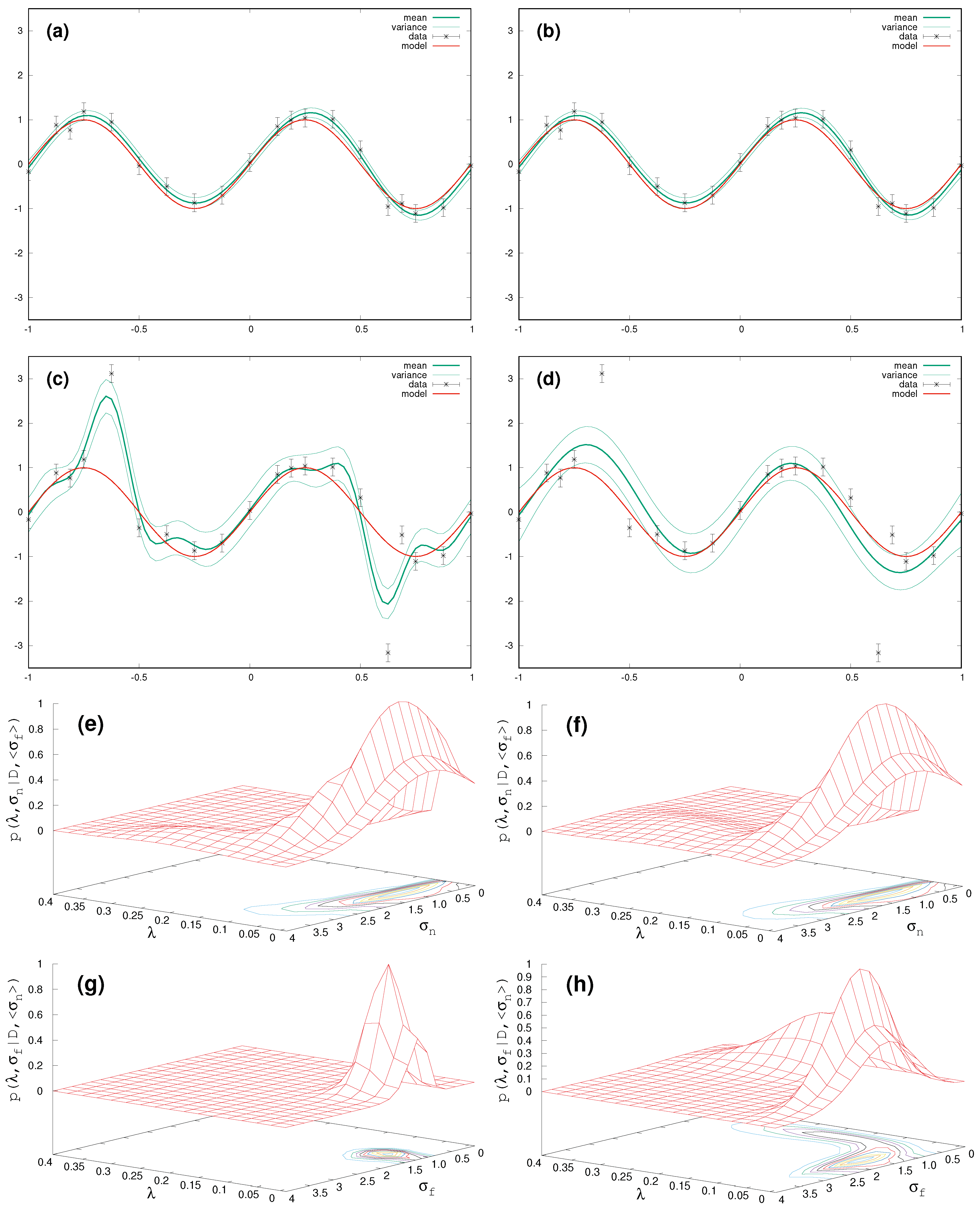
Figure 1 shows the results with the GP-method and the TP-method on the left and right panels, respectively. In the absence of outliers both methods give the same answer in Figure 1a,b. However, with two outliers at hand (two randomly chosen data points were raised by just multiplying with a factor of three), the surrogate from the GP-method (see Figure 1c) tries to follow each target value slavishly, which results in a smaller hyperparameter $\lambda$, equivalent to a bumpier behaviour. On the contrary, within the TP-method the outliers are more or less ignored but lead to a larger variance of the surrogate still clearly following a sin-function (see Figure 1d).

It is informative to have a look at the marginal likelihood for the hyperparameters $\mathbf{\theta }$. Since there are three hyperparameters, we employ two two-dimensional plots for ($\lambda$, ${\sigma }_n$) in Figure 1e,f and ($\lambda$, ${\sigma }_f$) in Figure 1g,h, where the respectively lacking third hyperparameter ${\sigma }_f$/${\sigma }_n$ for the first/second plot is kept constant in terms of its expectation value from integration over the marginal likelihood Equations (5) and (6), respectively. The most important differences are seen for ($\lambda$, ${\sigma }_f$), i.e., Figure 1g,h. In comparison with the GP-case, for $\lambda$ values around 0.05, the Student-t result shows a broader structure in ${\sigma }_f$, and for ${\sigma }_f$ around 0.5 an additional structure which comprises $\lambda$-values between [0.10,0.25]. The contributions in the marginal likelihood for this broad bump attributed to the larger $\lambda$-values between [0.10,0.25] are responsible for the smooth functional behaviour.

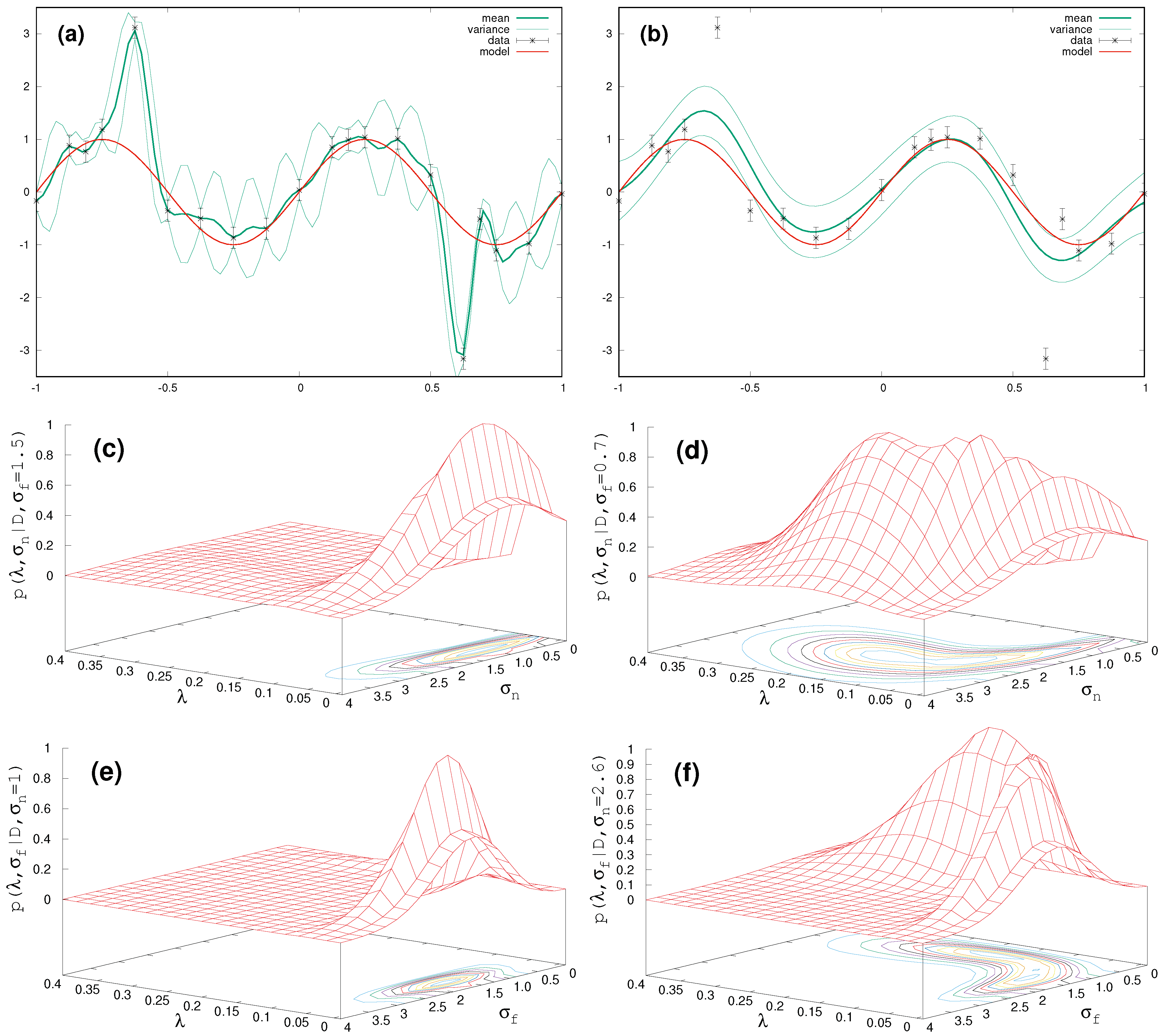
In order to examine these findings more thoroughly, in Figure 2, we focus on two settings of the hyperparameters deduced from the extremal structures in Figure 1h of the Student-t process. In the left panel, starting with Figure 2a for $\lambda$ = 0.05, ${\sigma }_f$ = 1.5, ${\sigma }_n$ = 1, a strong obedience to the target data is enforced. Therefore, the surfaces of the marginal likelihood, computed with either ${\sigma }_f$ = 1.5 (Figure 2c) or ${\sigma }_n$ = 1 (Figure 2e), get pinned down to a relatively small $\lambda$-variation. The situation changes in the right panel with $\lambda$ = 0.18, ${\sigma }_f$ = 0.7, ${\sigma }_n$ = 2.6, where we get broad structures for $\lambda$’s around 0.2 in connection with a somewhat more relaxed functional behaviour in Figure 2b.

From the above, it is clear that an MAP-solution would fail completely in the presence of outliers, because such an approach would focus on the maximum of the probability distribution at $max\lambda$ = 0.051 and $max{\sigma }_f$ = 1.61, thereby disregarding all contributions from the PDF for larger $\lambda$ along with smoother surrogates. Consequently, only the full exploitation of the marginal likelihood Equation (6) empowers the result to resemble the sin-function.

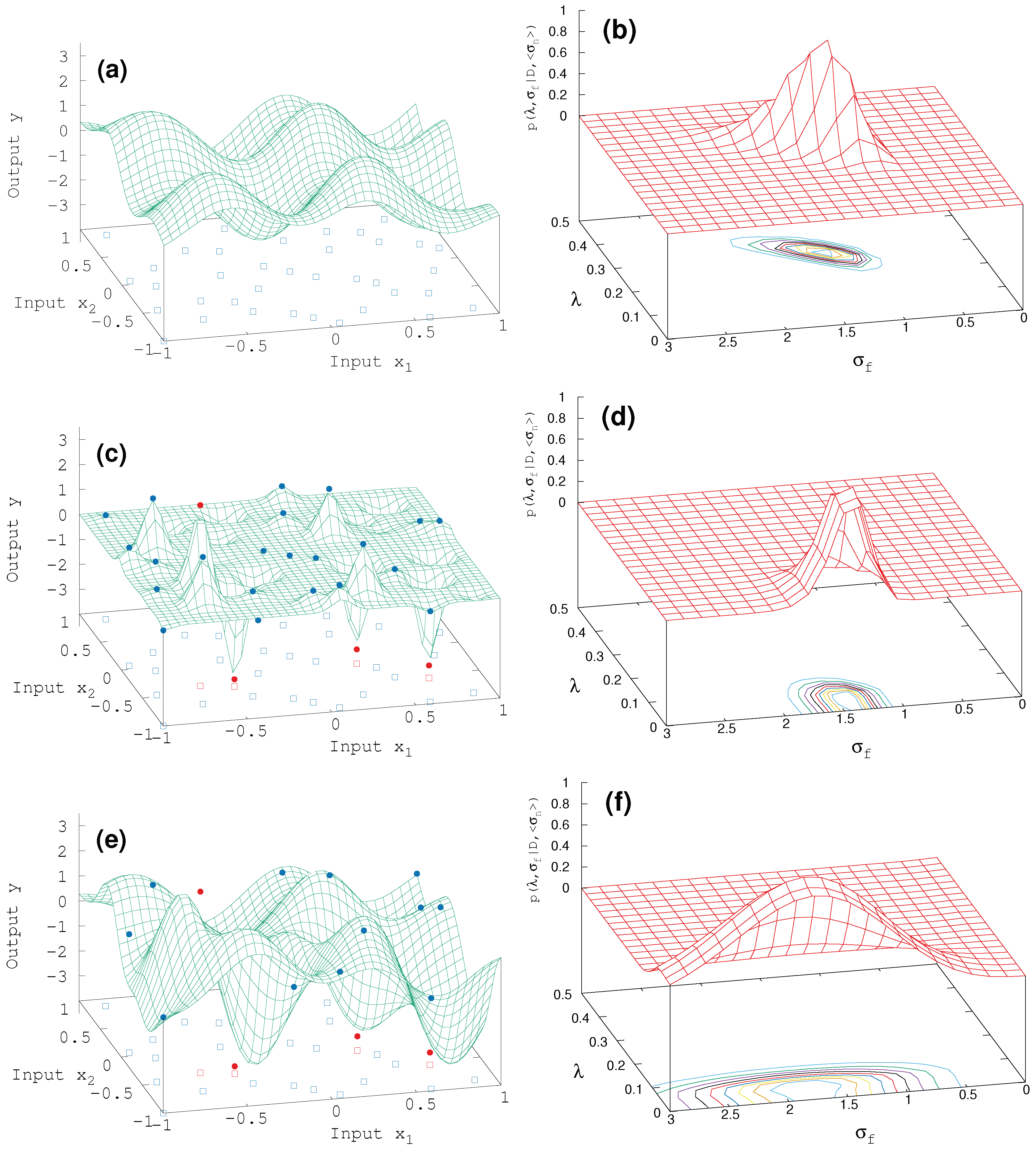
Next, we compare GP vs. TP in two dimensions (see Figure 3). A total of N = 40 target data are generated by the above double period sin-function just by expanding the x-dependence to x = ${(x_1,x_2)}^T$. Without outliers, the resulting surrogate surface (Figure 3a) is the same for GP and TP, revealing a mono-modal structure in hyperparametric space (Figure 3b) along with well defined expectation values with more or less concise variances, $\langle \lambda \rangle$ = 0.3 ± 0.04, $\langle {\sigma }_f\rangle$ = 1.3 ± 0.3, $\langle {\sigma }_n\rangle$ = 0.7 ± 0.4. It is certain that the MAP-approach would come to the same result for the surrogate surface.

The situation changes with outliers (N${}_{\mathrm{outlier}}$ = 4). The GP-surrogate (Figure 3c) fails completely and features a bump in the marginal likelihood (Figure 3c) which is confined around small $\lambda$-values below 0.1 and ${\sigma }_f\sim 1.4$. Compared with this, the TP-surrogate in Figure 3e resembles the sin model function where the mono-modal structure in the marginal likelihood widens (see Figure 3f), as already seen in the one-dimensional case.

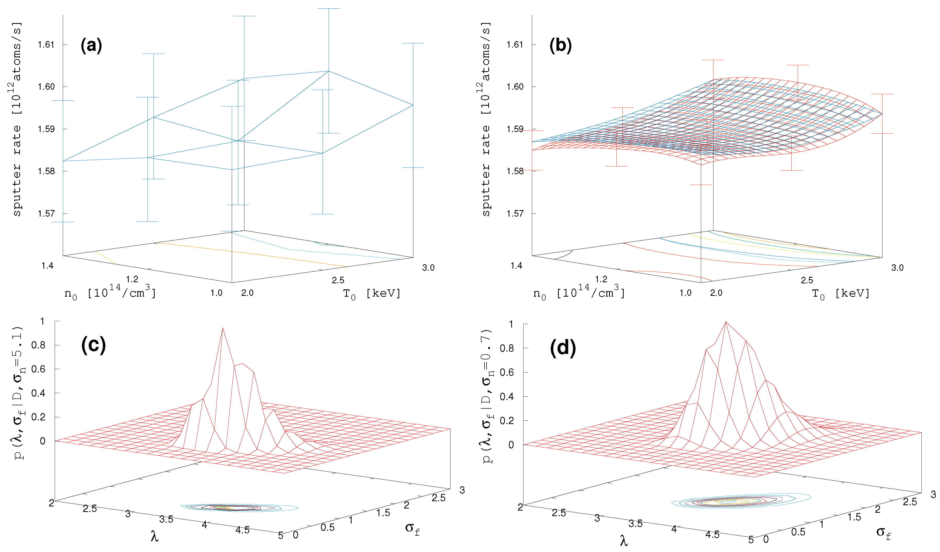
5. Results for Ion-Solid Interaction Simulations

Finally, we employ the data-analyzing tools characterized above to sputter rates generated by the ion-solid interaction simulations in a fusion plasma with EIRENE software [1]. To simulate these data, a total of 14 physics parameters are to be set on input. The most important parameters are those regarding electron density n and electron temperature T, both at two locations within the plasma, i.e., plasma center {$n_0$,$T_0$} and at the so-called pedestal {$n_{\mathrm{ped}}$,$T_{\mathrm{ped}}$} located at the plasma edge next to the separatix (last magnetic field line closed within the vessel). To begin with, we set up a test case with N = 3 × 3 × 3 × 3 = 81 EIRENE sputter rate data as function of these four parameters {$T_0,T_{\mathrm{ped}},n_0,n_{\mathrm{ped}}$} (results shown in Figure 4a).

In order to improve this apparently not very informative result on only a $3^4$ grid, we calculate the GP surrogate on a $5^4$-grid and take the $3^4$ data, being the worst in terms of variance, feed them back to EIRENE and take the resulting second $N_2$ = 81-data set (containing 11 doublets from initial one). This results in the initial one adding up to a total of $N_{\mathrm{tot}}=151$ data points. One can think of this as an iterative step, keeping the computation effort of the costly EIRENE runs low. The surrogate surfaces for the initial data set with N = 81 EIRENE data (blue mesh) and the full data set with $N_{\mathrm{tot}}$ = 151 (red mesh) are shown in Figure 4b, with the errorbars for the same nine data points as in Figure 4a. As can be seen, the iterative step reduces the uncertainty in the target by a factor of 3.6 (and misfit by factor of three). Moreover, while the surrogate surface (blue mesh) based on initial N = 81 EIRENE data shows only a maximal structure at $T_0=3$ keV smeared out around $n_0=1.26\times {10}^{14}$/cm${}^3$, the TP-surrogate surface (red mesh) has a clear maximum at $T_0=3$ keV and $n_0=1.20\times {10}^{14}$/cm${}^3$. The lower panel of Figure 4 shows the marginal likelihood surfaces for the hyperparameters $\lambda$, ${\sigma }_f$ for the results with N = 151 data. Since the TP-method (Figure 4d) shows a broader shape compared to the GP-method (Figure 4c), it may be inferred from the chapters above that the four-dimensional parameter space contains results for the sputter rates which do not fully obey a normally distributed uncertainty.

6. Conclusions

Exploring surrogate surfaces in multi-dimensional spaces has been proven to be employed advantageously by the Gaussian process (GP) method. For experimental data suffering from outliers, it is also known that the marginal posterior distribution can be made robust by acquiring, e.g., the Cauchy function instead of deferring to the Gaussian form. As shown in this paper, utilizing the Student-t process (TP) method can be performed by only a few and simple changes to an already well-established implementation of a GP-algorithm. The most important difference between both methods shows up in the marginal likelihood for the hyperparameters of the covariance function which—in the presence of outliers—becomes broader in the TP case compared to GP. The Bayesian method is to explore hyperparameter space by marginalization and let the data decide regarding the posterior probability distribution. However, with the basic assumption of normally distributed data, the GP method slavishly follows each data point within its variance, thereby generating a surrogate surface which irredeemably deteriorates in the presence of outliers. In a real world situation with occasionally faulty measurements, the TP-method offers the possibility of ignoring heavily distorted data by featuring a broader marginal probability distribution. Eventually, the TP-method improves the overall result for surrogate surfaces in comparison with Gaussian Processes and adds robustness with respect to outliers.