Graphical Gaussian Models Associated to a Homogeneous Graph with Permutation Symmetries ^†

Abstract

We consider multivariate-centered Gaussian models for the random vector $(Z^1,\dots ,Z^p)$, whose conditional structure is described by a homogeneous graph and which is invariant under the action of a permutation subgroup. The following paper is concerned with model selection within colored graphical Gaussian models, when the underlying conditional dependency graph is known. We derive an analytic expression of the normalizing constant of the Diaconis–Ylvisaker conjugate prior for the precision parameter and perform Bayesian model selection in the class of graphical Gaussian models invariant by the action of a permutation subgroup. We illustrate our results with a toy example of dimension 5.

1. Introduction

In the Graphical Gaussian model, conditional independencies among components of a random vector $Z=(Z^1,Z^2,\dots ,Z^p)$ obeying the multivariate centered Gaussian law $\mathrm{N}(0,\Sigma )$ with an unknown covariance matrix $\Sigma \in {\mathrm{Sym}}^{+}(p,\mathbb{R})$ are assigned by a simple undirected graph $\mathcal{G}=(\mathcal{V},\mathcal{E})$, where the set $\mathcal{V}$ of vertices is enumerated as $\mathcal{V}=\{1,2,\dots ,p\}$. Namely, if the vertices i and j are disconnected in the graph $\mathcal{G}$, then $Z^i$ and $Z^j$ are conditionally independent given other components $Z^k$, $k\ne i,j$. This property is equivalent to the $(i,j)$-component of the precision matrix $K:={\Sigma }^{-1}$ equals 0. Following Højsgaard and Lauritzen [1], we impose the invariance on such a statistical model under the natural action of a permutation subgroup $\Gamma \subset {\mathfrak{S}}_p$ preserving the conditional independence structure of the model, which means that $\Gamma$ is a subgroup of the automorphism group $\mathrm{Aut}\left(\mathcal{G}\right):=\left\{\sigma \in {\mathfrak{S}}_p;\sigma \left(i\right)\sim \sigma \left(j\right) \mathrm{if} \mathrm{and} \mathrm{only} \mathrm{if} i\sim j\right\}$ of the graph $\mathcal{G}$, where $i\sim j$ means that there exists an edge between the vertices i and j. Such models are called RCOP graphical models. It is proved that, when the graph $\mathcal{G}$ is homogeneous (i.e., decomposable and $A_4$-free, see [2]), the parameter set ${\mathcal{P}}_{\mathcal{G}}^{\Gamma }$ of precision matrices K of our invariant model forms a homogeneous cone. Therefore, we can apply our previous results [3] about the Wishart laws on homogeneous cones to this situation. In particular, we obtain an exact analytic formula for the normalizing constant of the Diaconis–Ylvisaker conjugate prior to the precision matrix. In order to demonstrate our results, we work on the data set of the examination marks of 88 students in 5 different mathematical subjects reported in Mardia et al. [4], following Højsgaard and Lauritzen [1]. As is discussed in Whittaker [5] and Edwards [6], the data fit into the graphical Gaussian model from Figure 1.

We carry out Bayesian model selection in the spirit of Graczyk et al. [7] of the group $\Gamma$ having the highest posterior probability among the ten possible groups preserving the graph above. We note that in [7], only complete graph $\mathcal{G}$ was allowed. Thanks to new formulas for the normalizing constant of Diaconis–Ylvisaker conjugate prior, we are able to generalize results of [7] to homogeneous graphs.

The authors are grateful to anonymous referees for their careful reading and valuable comments.

2. Main Results

Let us describe our results in more detail. Let ${\mathcal{Z}}_{\mathcal{G}}^{\Gamma }$ be the linear space consisting of symmetric matrices $K\in \mathrm{Sym}(p,\mathbb{R})$ such that $K_{\sigma \left(i\right)\sigma \left(j\right)}=K_{ij}$ for all $\sigma \in \Gamma$ and $i,j\in \mathcal{V}$, and $K_{ij}=0$ if $i\ne j$ and $i\neg \sim j$. Then the cone ${\mathcal{P}}_{\mathcal{G}}^{\Gamma }$ equals ${\mathcal{Z}}_{\mathcal{G}}^{\Gamma }\cap {\mathrm{Sym}}^{+}(p,\mathbb{R})$, so that our statistical model is the family of $N(0,\Sigma )$ with ${\Sigma }^{-1}\in {\mathcal{P}}_{\mathcal{G}}^{\Gamma }$. The Diaconis–Ylvisaker conjugate prior for $K={\Sigma }^{-1}\in {\mathcal{P}}_{\mathcal{G}}^{\Gamma }$ is given by

$$\begin{array}{c}\hfill f(K;\delta ,D):=\frac{1}{I_{\mathcal{G}}^{\Gamma }(\delta ,D)}{e}^{-\mathrm{tr}KD/2}{(detK)}^{(\delta -2)/2}{1}_{{\mathcal{P}}_{\mathcal{G}}^{\Gamma }}\left(K\right)\end{array}$$

(1)

for hyperparameters $\delta >2$ and $D\in {\mathrm{Sym}}^{+}(p,\mathbb{R})$, where

$$I_{\mathcal{G}}^{\Gamma }(\delta ,D):={\int }_{{\mathcal{P}}_{\mathcal{G}}^{\Gamma }}{e}^{-\mathrm{tr}KD/2}{(detK)}^{(\delta -2)/2}dK$$

is the normalizing constant. As is already stated, the cone ${\mathcal{P}}_{\mathcal{G}}^{\Gamma }$ is homogeneous, which means that there exists a linear group $H\subset GL\left({\mathcal{Z}}_{\mathcal{G}}^{\Gamma }\right)$ acting on ${\mathcal{P}}_{\mathcal{G}}^{\Gamma }$ transitively. Then, making use of our integral formula over ${\mathcal{P}}_{\mathcal{G}}^{\Gamma }$, see (2), we can compute the normalizing constant $I_{\mathcal{G}}^{\Gamma }(\delta ,D)$.

In order to state the integral formula, we introduce some functions. Let $\mathcal{Z}$ be a linear subspace of $\mathrm{Sym}(p,\mathbb{R})$ such that ${\mathcal{P}}_{\mathcal{Z}}:=\mathcal{Z}\cap {\mathrm{Sym}}^{+}(p,\mathbb{R})$ is non-empty. Let ${\pi }_{\mathcal{Z}}:\mathrm{Sym}(p,\mathbb{R})\to \mathcal{Z}$ denote the orthogonal projection with respect to the trace inner product $\langle x,y\rangle :=\mathrm{tr}xy$, $x,y\in \mathrm{Sym}(p,\mathbb{R})$, that is,

$$\langle x,y\rangle =\langle x,{\pi }_{\mathcal{Z}}\left(y\right)\rangle ,x\in \mathcal{Z},y\in \mathrm{Sym}(p,\mathbb{R}).$$

Let ${\mathcal{P}}_{\mathcal{Z}}^{*}$ be the dual cone of ${\mathcal{P}}_{\mathcal{Z}}$, that is, ${\mathcal{P}}_{\mathcal{Z}}^{*}:=\left\{y\in \mathcal{Z};\langle x,y\rangle >0 \mathrm{for} \mathrm{all} x\in \overline{{\mathcal{P}}_{\mathcal{Z}}}\backslash \left\{0\right\}\right\}.$ It is easy to see that, if $D\in {\mathrm{Sym}}^{+}(p,\mathbb{R})$, then ${\pi }_{\mathcal{Z}}\left(D\right)\in {\mathcal{P}}_{\mathcal{Z}}^{*}$. One can show that (see the proof of Proposition V.8 in [8]), for each $y\in {\mathcal{P}}_{\mathcal{Z}}^{*}$, there exists a unique ${\psi }_{\mathcal{Z}}\left(y\right)\in {\mathcal{P}}_{\mathcal{Z}}$ such that the function ${\mathcal{P}}_{\mathcal{Z}}\ni x\mapsto e^{-\langle x,y\rangle }detx$ attains its maximum value at $x={\psi }_{\mathcal{Z}}\left(y\right)$, and that the map ${\psi }_{\mathcal{Z}}:{\mathcal{P}}_{\mathcal{Z}}^{*}\to {\mathcal{P}}_{\mathcal{Z}}$ equals the inverse map of ${\mathcal{P}}_{\mathcal{Z}}\ni x\mapsto {\pi }_{\mathcal{Z}}\left(x^{-1}\right)\in {\mathcal{P}}_{\mathcal{Z}}^{*}$. For $y\in {\mathcal{P}}_{\mathcal{Z}}^{*}$, define ${\delta }_{\mathcal{Z}}\left(y\right):={(det{\psi }_{\mathcal{Z}}\left(y\right))}^{-1}$ and let $S_{\mathcal{Z}}\left(y\right):\mathcal{Z}\to \mathcal{Z}$ be a linear operator defined in such a way that

$$\langle S_{\mathcal{Z}}\left(y\right)u,v\rangle =-\left(\frac{{\partial }^2}{\partial s\partial t}\right)log{\delta }_{\mathcal{Z}}(y+su+tv){|}_{s=t=0}u,v\in \mathcal{Z}.$$

Namely, $S_{\mathcal{Z}}\left(y\right)$ is the Hessian operator of a strictly convex function $-log{\delta }_{\mathcal{Z}}\left(y\right)$. Put ${\phi }_{\mathcal{Z}}\left(y\right):={(det{S}_{\mathcal{Z}}\left(y\right))}^{1/2}$ for $y\in {\mathcal{P}}_{\mathcal{Z}}^{*}$. Finally, define ${\gamma }_{\mathcal{Z}}\left(\alpha \right):={\int }_{{\mathcal{P}}_{\mathcal{Z}}}{e}^{-\mathrm{tr}x}{(detx)}^{\alpha }dx$ for $\alpha \ge 0$, where $dx$ denotes the Lebesgue measure on $\mathcal{Z}$ normalized by the trace inner product. Namely, $dx={\prod }_{i=1}^{dim\mathcal{Z}}d{x}_i$, where $(x_1,\dots ,x_{dim\mathcal{Z}})$ is the standard coordinate system associated to an orthonormal basis of $\mathcal{Z}$ with respect to the trace inner product.

Theorem 1.

If $\mathcal{Z}={\mathcal{Z}}_{\mathcal{G}}^{\Gamma }$, then one has

$${\int }_{{\mathcal{P}}_{\mathcal{Z}}}{e}^{-\langle x,y\rangle }{(detx)}^{\alpha }dx={\gamma }_{\mathcal{Z}}\left(\alpha \right){\phi }_{\mathcal{Z}}\left(y\right){\delta }_{\mathcal{Z}}{\left(y\right)}^{-\alpha }y\in {\mathcal{P}}_{\mathcal{Z}}^{*},\alpha \ge 0.$$

(2)

We shall show Theorem 1 by using the homogeneity of ${\mathcal{P}}_{\mathcal{G}}^{\Gamma }={\mathcal{P}}_{{\mathcal{Z}}_{\mathcal{G}}^{\Gamma }}$ in our case, whereas we notice that the Formula (2) is also valid for some non-homogeneous cases, e.g., the cone ${\mathcal{P}}_{\mathcal{Z}}$ arising from uncolored decomposable graphical models [9].

Let ${\gamma }_{\mathcal{G}}^{\Gamma },{\delta }_{\mathcal{G}}^{\Gamma }$ and ${\phi }_{\mathcal{G}}^{\Gamma }$ denote the functions ${\gamma }_{\mathcal{Z}},{\delta }_{\mathcal{Z}}$ and ${\phi }_{\mathcal{Z}}$, respectively, with $\mathcal{Z}={\mathcal{Z}}_{\mathcal{G}}^{\Gamma }$. Then, we have

$$I_{\mathcal{G}}^{\Gamma }(\delta ,D)={\gamma }_{\mathcal{G}}^{\Gamma }((\delta -2)/2){\phi }_{\mathcal{G}}^{\Gamma }({\pi }_{\mathcal{Z}}\left(D\right)/2){\delta }_{\mathcal{G}}^{\Gamma }{({\pi }_{\mathcal{Z}}\left(D\right)/2)}^{-(\delta -2)/2}.$$

In our Bayesian model selection setting [7], for a fixed graph $\mathcal{G}$, we suppose that a group $\Gamma$ is distributed uniformly over all the possible subgroups of the automorphism group of the graph $\mathcal{G}$. Given samples $Z_1,Z_2,\cdots ,Z_n$, that is, the independent and identically distributed random vectors obeying $N(0,\Sigma )$ with ${\Sigma }^{-1}\in {\mathcal{P}}_{\mathcal{G}}^{\Gamma }$, we see that the posterior probability $\mathbb{P}(\Gamma |Z_1,\dots ,Z_n)$ is proportional to $I_{\mathcal{G}}^{\Gamma }(\delta +n,D+{\sum }_{i=1}^n{Z}_i{Z}_i^{\top })/I_{\mathcal{G}}^{\Gamma }(\delta ,D)$, see [7] (Equation (30)).

3. Matrix Realization of Homogeneous Cones

It is known that any homogeneous cone is linearly isomorphic to some ${\mathcal{P}}_{\mathcal{Z}}$, where $\mathcal{Z}\subset \mathrm{Sym}(p,\mathbb{R})$ is a linear subspace consisting of real symmetric matrices admitting certain specific block decompositions described below [10,11]. Let $n_1,n_2,\dots ,n_r$ be positive integers such that $p=n_1+n_2+\dots +n_r$. Let $V={\left\{V_{lk}\right\}}_{1\le k<l\le r}$ be a family of linear spaces $V_{lk}\subset \mathrm{Mat}(n_l,n_k;\mathbb{R})$ satisfying the following axioms:

• (V1) $A\in V_{lk}\Rightarrow A{A}^{\top }\in \mathbb{R}{I}_{n_l}(1\le k<l\le r)$,
• (V2) $A\in V_{lj},B\in V_{kj}\Rightarrow A{B}^{\top }\in V_{lk}(1\le j<k<l\le r)$,
• (V3) $A\in V_{lk},B\in V_{kj}\Rightarrow AB\in V_{lj}(1\le j<k<l\le r)$.

Let ${\mathcal{Z}}_V$ be the linear space consisting of $x\in \mathrm{Sym}(p,\mathbb{R})$ of the following form:

$$x=\left(\begin{array}{cccc}{X}_{11}& X_{21}^{\top }& \cdots & X_{r1}^{\top }\\ X_{21}& X_{22}& & X_{r2}^{\top }\\ ⋮& & \ddots & ⋮\\ X_{r1}& X_{r2}& \cdots & X_{rr}\end{array}\right)\begin{array}{cc}\hfill X_{kk}& =x_{kk}{I}_{n_k},x_{kk}\in \mathbb{R},k=1,\dots ,r,\hfill \\ \hfill X_{lk}& \in V_{lk},1\le k<l\le r.\hfill \end{array}$$

(3)

Let $H_V$ be the set of $p\times p$ lower triangular matrices T of the following form:

$$T=\left(\begin{array}{cccc}{T}_{11}& & & \\ T_{21}& T_{22}& & \\ ⋮& & \ddots & \\ T_{r1}& T_{r2}& \cdots & T_{rr}\end{array}\right)\begin{array}{cc}\hfill T_{kk}& =t_{kk}{I}_{n_k},t_{kk}>0,k=1,\dots ,r,\hfill \\ \hfill T_{lk}& \in V_{lk},1\le k<l\le r.\hfill \end{array}$$

(4)

Then, $H_V$ forms a Lie group by (V3), and acts on ${\mathcal{Z}}_V$ linearly by $\rho \left(T\right)x:=Tx{T}^{\top }$, $T\in H_V$, $x\in {\mathcal{Z}}_V$. Moreover, the group $H_V$ acts on the cone ${\mathcal{P}}_V:={\mathcal{P}}_{{\mathcal{Z}}_V}$ simply transitively by $\rho$. We write ${\rho }^{*}\left(T\right)$, $T\in H_V$, for the adjoint of the linear operator $\rho \left(T\right)$ on ${\mathcal{Z}}_V$ with respect to the trace inner product, which means that $\langle \rho \left(T\right)x,y\rangle =\langle x,{\rho }^{*}\left(T\right)y\rangle$ for $x,y\in {\mathcal{Z}}_V$. Then, we see that ${\rho }^{*}\left(T\right)y={\pi }_{\mathcal{Z}}\left(T^{\top }yT\right)$ for $y\in {\mathcal{Z}}_V$. Moreover, if $y\in {\mathcal{P}}_V^{*}:={\mathcal{P}}_{{\mathcal{Z}}_V}^{*}$, we have ${\psi }_{{\mathcal{Z}}_V}\left({\rho }^{*}\left(T\right)y\right)=\rho \left(T^{-1}\right){\psi }_{{\mathcal{Z}}_V}\left(y\right)$. Since ${\psi }_{\mathcal{Z}}\left(y\right)\in {\mathcal{P}}_V$ for $y\in {\mathcal{P}}_V^{*}$, we can take a unique $T_y\in H_V$ for which ${\psi }_{\mathcal{Z}}\left(y\right)=\rho \left(T_y^{-1}\right)I_p$. Then, we have $y={\rho }^{*}\left(T_y\right)I_p$ because $\rho \left(T_y^{-1}\right)I_p=\rho \left(T_y^{-1}\right){\psi }_{\mathcal{Z}}\left(I_p\right)={\psi }_{\mathcal{Z}}\left({\rho }^{*}\left(T_y\right)I_p\right)$.

Lemma 1.

For $y\in {\mathcal{P}}_{{\mathcal{Z}}_V}^{*}$, one has ${\delta }_{{\mathcal{Z}}_V}\left(y\right)={(det{T}_y)}^2$ and ${\phi }_{{\mathcal{Z}}_V}\left(y\right)={(det\rho \left(T_y\right))}^{-1}$.

Using Lemma 1 and a general theory about relatively invariant functions on a homogeneous cone (see, e.g., [10] (Section IV)), we can compute explicitly ${\delta }_{{\mathcal{Z}}_V}$ and ${\phi }_{{\mathcal{Z}}_V}$.

Put $q_k:={\sum }_{l>k}dim{V}_{lk}$ for $k=1,\dots ,r$ and $N:=dim{\mathcal{Z}}_V$.

Theorem 2.

(i) One has

$${\gamma }_{{\mathcal{Z}}_V}\left(\alpha \right)={\left(2\pi \right)}^{(N-r)/2}\prod _{k=1}^r\left(n_k^{-n_k\alpha -(q_k+1)/2}\Gamma (n_k\alpha +(q_k/2)+1)\right).$$

(ii) The equality (2) holds for $\mathcal{Z}={\mathcal{Z}}_V$.

We give a sketch of the proof of Theorem 2. We denote by $\left(A\right|B)$ the trace inner product $\mathrm{tr}A{B}^{\top }$ of $A,B\in V_{lk}$. Then, for an element $x\in {\mathcal{Z}}_V$ in (3), we have

$$\langle x,x\rangle =\sum _{k=1}^r\left(n_k{x}_{kk}^2\right)+2\sum _{1\le k<l\le r}\left(X_{lk}\right|X_{lk}),$$

so that $dx={\prod }_{k=1}^r\left(n_k^{1/2}d{x}_{kk}\right){\prod }_{1\le k<l\le r}\left(2^{dim{V}_{lk}/2}d{X}_{lk}\right),$ where $d{X}_{lk}$ stands for the Lebesgue measure on $V_{lk}$ normalized by $(·|·)$. By the change of variable $x=\rho \left(T\right)I_p$ with $T\in H_V$ in (4), we get

$$dx=\prod _{k=1}^r\left(n_k^{1/2}2t_{kk}^{1+q_k}d{t}_{kk}\right)\prod _{1\le k<l\le r}{2}^{dim{V}_{lk}/2}d{T}_{lk},$$

so that ${\gamma }_{{\mathcal{Z}}_V}\left(\alpha \right)$ equals

$$\begin{array}{c}\hfill \prod _{k=1}^r\left({\int }_0^{\infty }{e}^{-n_k{t}_{kk}^2}{n}_k^{1/2}2t_{kk}^{2n_k\alpha +1+q_k}d{t}_{kk}\right)\prod _{1\le k<l\le r}\left(2^{dim{V}_{lk}/2}{\int }_{V_{lk}}{e}^{-\left(T_{lk}\right|T_{lk})}d{T}_{lk}\right).\end{array}$$

As for (ii), we observe that $\langle x,y\rangle =\langle x,{\rho }^{*}\left(T_y\right)I_p\rangle =\langle \rho \left(T_y\right)x,I_p\rangle =\mathrm{tr}\rho \left(T_y\right)x.$ By the change of variable $x^{\prime }=\rho \left(T_y\right)x$, we have

$$\begin{array}{cc}\hfill {\int }_{{\mathcal{P}}_V}{e}^{-\langle x,y\rangle }{(detx)}^{\alpha }dx& ={\int }_{{\mathcal{P}}_V}{e}^{-\mathrm{tr}{x}^{\prime }}{\left\{(det{x}^{\prime }){(det{T}_y)}^{-2}\right\}}^{\alpha }{(det\rho \left(T_y\right))}^{-1}d{x}^{\prime }\hfill \\ \hfill & ={(det{T}_y)}^{-2\alpha }{(det\rho \left(T_y\right))}^{-1}{\gamma }_{{\mathcal{Z}}_V}\left(\alpha \right),\hfill \end{array}$$

so that (2) follows from Lemma 1.

Theorem 3.

For a homogeneous graph $\mathcal{G}=(\mathcal{V},\mathcal{E})$ and a subgroup Γ of the automorphism group of $\mathcal{G}$, there exists an orthogonal matrix $U\in O\left(p\right)$ such that $U^{\top }{\mathcal{Z}}_{\mathcal{G}}^{\Gamma }U={\mathcal{Z}}_V$ with some $V={\left\{V_{lk}\right\}}_{1\le k<l\le r}$.

The proof is omitted; it is based on a representation theory similarly as in [7] and uses a proper ordering of vertices. Theorem 3 together with Theorem 2 yields Theorem 1. Theorem 3 is very important from the practical point of view. The knowledge of the orthogonal matrix U allows us to identify all parameters of the space ${\mathcal{Z}}_V$ (see (3)). However, the problem of finding a suitable U matrix is in general very complicated. In the next section, we will consider the butterfly model from Figure 1 and present the exact forms of the U matrices for all subgroups of $\mathrm{Aut}\left(\mathcal{G}\right)$.

4. Toy Example

In what follows, let $\mathcal{G}$ be the five-vertex graph from Figure 1. We use the cyclic representation of permutations on $\mathcal{V}=\{1,\dots ,5\}$. Then, the group $\mathrm{Aut}\left(\mathcal{G}\right)$ is generated by ${\sigma }_1:=\left(\begin{array}{cc}1& 2\end{array}\right),{\sigma }_2:=\left(\begin{array}{cc}4& 5\end{array}\right)$, and ${\sigma }_3:=\left(\begin{array}{cc}1& 4\end{array}\right)\left(\begin{array}{cc}2& 5\end{array}\right)$. Put $\tau :={\sigma }_2\circ {\sigma }_3=\left(\begin{array}{cccc}1& 5& 2& 4\end{array}\right)$. Then, ${\sigma }_2={\sigma }_1\circ {\tau }^2$ and ${\sigma }_3={\sigma }_1\circ {\tau }^3$, so that $\mathrm{Aut}\left(\mathcal{G}\right)$ is generated by ${\sigma }_1$ and $\tau$. Moreover, since the orders of ${\sigma }_1$ and $\tau$ are 2 and 4, respectively, with ${\sigma }_1\circ \tau \circ {\sigma }_1^{-1}={\tau }^3$, the group $\mathrm{Aut}\left(\mathcal{G}\right)$ equals the dihedral group $\langle {\sigma }_1\rangle ⋉\langle \tau \rangle$ of order 8. Then, all the subgroups of $\mathrm{Aut}\left(\mathcal{G}\right)$ are listed as:

$$\begin{array}{c}{\Gamma }_1:=\left\{e\right\},{\Gamma }_2:=\langle {\sigma }_1\rangle ,{\Gamma }_3:=\langle {\sigma }_1\circ \tau \rangle ,{\Gamma }_4:=\langle {\sigma }_1\circ {\tau }^2\rangle ,{\Gamma }_5:=\langle {\sigma }_1\circ {\tau }^3\rangle ,\\ {\Gamma }_6:=\langle {\tau }^2\rangle ,{\Gamma }_7:=\langle \tau \rangle ,{\Gamma }_8:=\langle {\sigma }_1,{\tau }^2\rangle ,{\Gamma }_9:=\langle {\sigma }_1\circ \tau ,{\tau }^2\rangle ,{\Gamma }_{10}:=\mathrm{Aut}\left(\mathcal{G}\right).\end{array}$$

(i) When $\Gamma ={\Gamma }_1$, then $x\in {\mathcal{Z}}_{\mathcal{G}}^{\Gamma }$ is of the form

$$x=\left(\begin{array}{ccccc}{x}_{11}& x_{21}& x_{31}& 0& 0\\ x_{21}& x_{22}& x_{32}& 0& 0\\ x_{31}& x_{32}& x_{33}& x_{43}& x_{53}\\ 0& 0& x_{43}& x_{44}& x_{54}\\ 0& 0& x_{53}& x_{54}& x_{55}\end{array}\right).$$

We give an orthogonal matrix U so that $U^{\top }xU$ becomes of the form of matrix realization in the previous section (see Theorem 3) by

$$U:=\left(\begin{array}{ccccc}1& 0& 0& 0& 0\\ 0& 1& 0& 0& 0\\ 0& 0& 0& 0& 1\\ 0& 0& 1& 0& 0\\ 0& 0& 0& 1& 0\end{array}\right),U^{\top }xU=\left(\begin{array}{ccccc}{x}_{11}& x_{21}& 0& 0& x_{31}\\ x_{21}& x_{22}& 0& 0& x_{32}\\ 0& 0& x_{44}& x_{54}& x_{43}\\ 0& 0& x_{54}& x_{55}& x_{53}\\ x_{31}& x_{32}& x_{43}& x_{53}& x_{33}\end{array}\right).$$

In this case, $N=11,r=5,n_1=\dots =n_5=1$, and $V_{lk}(1\le k<l\le 5)$ is $\mathbb{R}$ or $\left\{0\right\}$. Since ${\gamma }_{U^{\top }\mathcal{Z}U}\left(\alpha \right)={\gamma }_{\mathcal{Z}}\left(\alpha \right)$ in general, we see from Theorem 2 (i) that

$${\gamma }_{\mathcal{G}}^{\Gamma }\left(\alpha \right)={\left(2\pi \right)}^3\Gamma (\alpha +1)\Gamma {(\alpha +\frac{3}{2})}^2\Gamma {(\alpha +2)}^2.$$

Moreover, the functions ${\delta }_{\mathcal{G}}^{\Gamma }\left(x\right)$ and ${\phi }_{\mathcal{G}}^{\Gamma }\left(x\right)$ are expressed, respectively, as

$$x_{33}^{-1}\left|\begin{array}{ccc}{x}_{11}& x_{21}& x_{31}\\ x_{21}& x_{22}& x_{32}\\ x_{31}& x_{32}& x_{33}\end{array}\right|\left|\begin{array}{ccc}{x}_{33}& x_{43}& x_{53}\\ x_{43}& x_{44}& x_{54}\\ x_{53}& x_{54}& x_{55}\end{array}\right|,x_{33}{\left|\begin{array}{ccc}{x}_{11}& x_{21}& x_{31}\\ x_{21}& x_{22}& x_{32}\\ x_{31}& x_{32}& x_{33}\end{array}\right|}^{-2}{\left|\begin{array}{ccc}{x}_{33}& x_{43}& x_{53}\\ x_{43}& x_{44}& x_{54}\\ x_{53}& x_{54}& x_{55}\end{array}\right|}^{-2}.$$

For $i=2,\dots ,10$, clearly ${\mathcal{P}}_{\mathcal{G}}^{{\Gamma }_i}$ is a subset of ${\mathcal{P}}_{\mathcal{G}}^{\Gamma }={\mathcal{P}}_{\mathcal{G}}^{{\Gamma }_1}$ and one can show that ${\delta }_{\mathcal{G}}^{{\Gamma }_i}$ is equal to the restriction of ${\delta }_{\mathcal{G}}^{\Gamma }$ above to ${\mathcal{P}}_{\mathcal{G}}^{{\Gamma }_i}$.

(ii) When $\Gamma ={\Gamma }_2$, we describe, respectively, $x\in {\mathcal{Z}}_{\mathcal{G}}^{\Gamma }$, an orthogonal matrix U and $U^{\top }xU$ as

$$\left(\begin{array}{ccccc}a& b& c& 0& 0\\ b& a& c& 0& 0\\ c& c& d& e& f\\ 0& 0& e& g& h\\ 0& 0& f& h& i\end{array}\right),\left(\begin{array}{ccccc}1/\sqrt{2}& 1/\sqrt{2}& 0& 0& 0\\ -1/\sqrt{2}& 1/\sqrt{2}& 0& 0& 0\\ 0& 0& 0& 0& 1\\ 0& 0& 1& 0& 0\\ 0& 0& 0& 1& 0\end{array}\right),\left(\begin{array}{ccccc}a-b& 0& 0& 0& 0\\ 0& a+b& 0& 0& \sqrt{2}c\\ 0& 0& g& h& e\\ 0& 0& h& i& f\\ 0& \sqrt{2}c& e& f& d\end{array}\right).$$

We have ${\gamma }_{\mathcal{G}}^{\Gamma }\left(\alpha \right)={\left(2\pi \right)}^2\Gamma {(\alpha +1)}^2\Gamma {(\alpha +\frac{3}{2})}^2\Gamma (\alpha +2)$, and

$${\phi }_{\mathcal{G}}^{\Gamma }\left(x\right)=d{(a-b)}^{-1}{\left|\begin{array}{cc}a+b& \sqrt{2}c\\ \sqrt{2}c& d\end{array}\right|}^{-3/2}{\left|\begin{array}{ccc}d& e& f\\ e& g& h\\ f& h& i\end{array}\right|}^{-2}.$$

(iii) When $\Gamma ={\Gamma }_3$, we describe, respectively, $x\in {\mathcal{Z}}_{\mathcal{G}}^{\Gamma }$, an orthogonal matrix U and $U^{\top }xU$ as

$$\left(\begin{array}{ccccc}a& d& e& 0& 0\\ d& b& f& 0& 0\\ e& f& c& f& e\\ 0& 0& f& b& d\\ 0& 0& e& d& a\end{array}\right),\left(\begin{array}{ccccc}1& 0& 0& 0& 0\\ 0& 0& 1& 0& 0\\ 0& 0& 0& 0& 1\\ 0& 0& 0& 1& 0\\ 0& 1& 0& 0& 0\end{array}\right),\left(\begin{array}{ccccc}a& 0& d& 0& e\\ 0& a& 0& d& e\\ d& 0& b& 0& f\\ 0& d& 0& b& f\\ e& e& f& f& c\end{array}\right).$$

Then ${\gamma }_{\mathcal{G}}^{\Gamma }\left(\alpha \right)={\left(2\pi \right)}^{3/2}{2}^{-4\alpha -5/2}\Gamma (2\alpha +2)\Gamma (2\alpha +\frac{3}{2})\Gamma (\alpha +1)$ and ${\phi }_{\mathcal{G}}^{\Gamma }\left(x\right)={\left|\begin{array}{ccc}a& d& e\\ d& b& f\\ e& f& c\end{array}\right|}^{-2}.$

(iv) When $\Gamma ={\Gamma }_4$, we describe, respectively, $x\in {\mathcal{Z}}_{\mathcal{G}}^{\Gamma }$, an orthogonal matrix U and $U^{\top }xU$ as

$$\left(\begin{array}{ccccc}a& d& e& 0& 0\\ d& b& f& 0& 0\\ e& f& c& g& g\\ 0& 0& g& h& i\\ 0& 0& g& i& h\end{array}\right),\left(\begin{array}{ccccc}1& 0& 0& 0& 0\\ 0& 1& 0& 0& 0\\ 0& 0& 0& 0& 1\\ 0& 0& 1/\sqrt{2}& 1/\sqrt{2}& 0\\ 0& 0& -1/\sqrt{2}& 1/\sqrt{2}& 0\end{array}\right),\left(\begin{array}{ccccc}a& d& 0& 0& e\\ d& b& 0& 0& f\\ 0& 0& h-i& 0& 0\\ 0& 0& 0& h+i& \sqrt{2}g\\ e& f& 0& \sqrt{2}g& c\end{array}\right).$$

Then, ${\gamma }_{\mathcal{G}}^{\Gamma }\left(\alpha \right)={\gamma }_{\mathcal{G}}^{{\Gamma }_2}\left(\alpha \right)={\left(2\pi \right)}^2\Gamma {(\alpha +1)}^2\Gamma {(\alpha +\frac{3}{2})}^2\Gamma (\alpha +2)$, while ${\phi }_{\mathcal{G}}^{\Gamma }\left(x\right)$ is equal to

$$c{(h-i)}^{-1}{\left|\begin{array}{cc}h+i& \sqrt{2}g\\ \sqrt{2}g& c\end{array}\right|}^{-3/2}{\left|\begin{array}{ccc}a& d& e\\ d& b& f\\ e& f& c\end{array}\right|}^{-2}.$$

(v) When $\Gamma ={\Gamma }_5$, we describe, respectively, $x\in {\mathcal{Z}}_{\mathcal{G}}^{\Gamma }$, an orthogonal matrix U and $U^{\top }xU$ as

$$\left(\begin{array}{ccccc}a& d& e& 0& 0\\ d& b& f& 0& 0\\ e& f& c& e& f\\ 0& 0& e& a& d\\ 0& 0& f& d& b\end{array}\right),\left(\begin{array}{ccccc}1& 0& 0& 0& 0\\ 0& 0& 1& 0& 0\\ 0& 0& 0& 0& 1\\ 0& 1& 0& 0& 0\\ 0& 0& 0& 1& 0\end{array}\right),\left(\begin{array}{ccccc}a& 0& d& 0& e\\ 0& a& 0& d& e\\ d& 0& b& 0& f\\ 0& d& 0& b& f\\ e& e& f& f& c\end{array}\right).$$

Then, ${\gamma }_{\mathcal{G}}^{\Gamma }\left(\alpha \right)={\gamma }_{\mathcal{G}}^{{\Gamma }_3}\left(\alpha \right)={\left(2\pi \right)}^{3/2}{2}^{-4\alpha -5/2}\Gamma (2\alpha +2)\Gamma (2\alpha +\frac{3}{2})\Gamma (\alpha +1)$ and ${\phi }_{\mathcal{G}}^{\Gamma }\left(x\right)={\left|\begin{array}{ccc}a& d& e\\ d& b& f\\ e& f& c\end{array}\right|}^{-2}.$

(vi) We have ${\mathcal{Z}}_{\mathcal{G}}^{{\Gamma }_6}={\mathcal{Z}}_{\mathcal{G}}^{{\Gamma }_8}$. When $\Gamma ={\Gamma }_6$ or ${\Gamma }_8$, we describe, respectively, $x\in {\mathcal{Z}}_{\mathcal{G}}^{\Gamma }$, an orthogonal matrix U and $U^{\top }xU$ as

$$\begin{array}{c}\left(\begin{array}{ccccc}a& b& c& 0& 0\\ b& a& c& 0& 0\\ c& c& d& e& e\\ 0& 0& e& f& g\\ 0& 0& e& g& f\end{array}\right),\left(\begin{array}{ccccc}1/\sqrt{2}& 1/\sqrt{2}& 0& 0& 0\\ -1/\sqrt{2}& 1/\sqrt{2}& 0& 0& 0\\ 0& 0& 0& 0& 1\\ 0& 0& 1/\sqrt{2}& 1/\sqrt{2}& 0\\ 0& 0& -1/\sqrt{2}& 1/\sqrt{2}& 0\end{array}\right),\\ \left(\begin{array}{ccccc}a-b& 0& 0& 0& 0\\ 0& a+b& 0& 0& \sqrt{2}c\\ 0& 0& f-g& 0& 0\\ 0& 0& 0& f+g& \sqrt{2}e\\ 0& \sqrt{2}c& 0& \sqrt{2}e& d\end{array}\right).\end{array}$$

Then, ${\gamma }_{\mathcal{G}}^{\Gamma }\left(\alpha \right)=2\pi \Gamma {(\alpha +1)}^3\Gamma {(\alpha +\frac{3}{2})}^2$, and

$${\phi }_{\mathcal{G}}^{\Gamma }\left(x\right)=d{(a-b)}^{-1}{(f-g)}^{-1}{\left|\begin{array}{cc}a+b& \sqrt{2}c\\ \sqrt{2}c& d\end{array}\right|}^{-3/2}{\left|\begin{array}{cc}f+g& \sqrt{2}e\\ \sqrt{2}e& d\end{array}\right|}^{-3/2}.$$

(vii) For $\Gamma ={\Gamma }_7,{\Gamma }_9$ or ${\Gamma }_{10}$ the linear space ${\mathcal{Z}}_{\mathcal{G}}^{\Gamma }$ is the same. We describe, respectively, $x\in {\mathcal{Z}}_{\mathcal{G}}^{\Gamma }$, an orthogonal matrix U and $U^{\top }xU$ as

$$\begin{array}{c}\left(\begin{array}{ccccc}a& c& d& 0& 0\\ c& a& d& 0& 0\\ d& d& b& d& d\\ 0& 0& d& a& c\\ 0& 0& d& c& a\end{array}\right),\left(\begin{array}{ccccc}1/\sqrt{2}& 0& 1/\sqrt{2}& 0& 0\\ -1/\sqrt{2}& 0& 1/\sqrt{2}& 0& 0\\ 0& 0& 0& 0& 1\\ 0& -1/\sqrt{2}& 0& 1/\sqrt{2}& 0\\ 0& 1/\sqrt{2}& 0& 1/\sqrt{2}& 0\end{array}\right),\\ \left(\begin{array}{ccccc}a-c& 0& 0& 0& 0\\ 0& a-c& 0& 0& 0\\ 0& 0& a+c& 0& \sqrt{2}d\\ 0& 0& 0& a+c& \sqrt{2}d\\ 0& 0& \sqrt{2}d& \sqrt{2}d& b\end{array}\right).\end{array}$$

Then, ${\gamma }_{\mathcal{G}}^{\Gamma }\left(\alpha \right)={\left(2\pi \right)}^{1/2}{2}^{-4\alpha -3/2}\Gamma (2\alpha +1)\Gamma (2\alpha +\frac{3}{2})\Gamma (\alpha +1)$ and ${\phi }_{\mathcal{G}}^{\Gamma }\left(x\right)={(a-c)}^{-1}$${\left|\begin{array}{cc}a+c& \sqrt{2}d\\ \sqrt{2}d& b\end{array}\right|}^{-3/2}.$

5. Numerical Example

We carry out Bayesian model selection in the spirit of Graczyk et al. [7]. For a fixed graph $\mathcal{G}$, we suppose that a group $\Gamma$ is distributed uniformly over all possible subgroups of $\mathrm{Aut}\left(\mathcal{G}\right)$. Given sample $Z_1,\dots ,Z_n$ from $\mathrm{N}(0,\Sigma )$ with ${\Sigma }^{-1}\in {\mathcal{P}}_{\mathcal{G}}^{\Gamma }$, where $K={\Sigma }^{-1}$ follows the Diaconis–Ylvisaker conjugate prior (1) with hyperparameters $(\delta ,D)$, then the posterior probability $\mathbb{P}(\Gamma |Z_1,\dots ,Z_n)$ is proportional to $I_{\mathcal{G}}^{\Gamma }(\delta +n,D+{\sum }_{i=1}^n{Z}_i{Z}_i^{\top })/I_{\mathcal{G}}^{\Gamma }(\delta ,D)$. In order to demonstrate our results, we work on the data set of the examination marks of $n=88$ students in $p=5$ different mathematical subjects. As was reported in [5,6], the data demonstrate an excellent fit to the graphical Gaussian model displayed in Figure 1. Since the groups $\Gamma ={\Gamma }_6,{\Gamma }_8$ (similarly ${\Gamma }_7$, ${\Gamma }_9$ and ${\Gamma }_{10}$) impose the same symmetries on ${\mathcal{Z}}_{\mathcal{G}}^{\Gamma }$, we consider Bayesian model selection within 7 different models: ${\Gamma }_i$ for $i=1,2,\dots ,7$. The five mathematical subjects are enumerated as in the graph presented in Figure 1. As our method applies only to centered normal sample, as usual, we center the marks and consider a correction of the degrees of freedom $n^{*}=88-1=87$. Then,

$$\sum _{i=1}^n{Z}_i{Z}_i^{\top }=\left(\begin{array}{ccccc}26601.82& 11068.36& 8837.41& 9245.73& 10214.23\\ 11068.36& 15037.27& 7408.68& 8236.55& |8614.05\\ 8837.41& 7408.68& 9821.08& 9753.86& 10602.74\\ 9245.73& 8236.55& 9753.86& 19173.09& 13531.59\\ 10214.23& 8614.05& 10602.74& 13531.59& 25904.72\end{array}\right).$$

We take usual hyperparameter $\delta =3$ and $D=d·I_5$ for $d\in \{1,{10}^2,{10}^4\}$. Below, we present a subgroup with the highest posterior probability p.

$$\begin{array}{ccc}d=1& d=100& d=10000\\ {\Gamma }_7(p=1)& {\Gamma }_3(p=0.8)& {\Gamma }_1(p=0.75)\end{array}$$

Depending on the value of hyperparameter D, the model with the highest posterior probability is

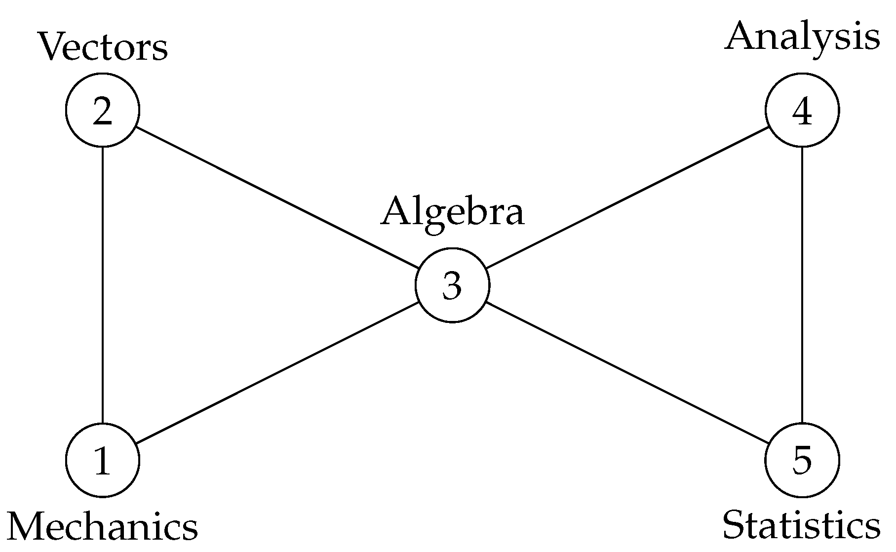
• ${\Gamma }_7$, which corresponds to full symmetry as ${\mathcal{Z}}_{\mathcal{G}}^{{\Gamma }_7}={\mathcal{Z}}_{\mathcal{G}}^{\mathrm{Aut}\left(\mathcal{G}\right)}$,
• ${\Gamma }_3=〈\left(\begin{array}{cc}1& 5\end{array}\right)\left(\begin{array}{cc}2& 4\end{array}\right)〉$, which corresponds to invariance of the model to interchange (Mechanics, Vectors) ↔ (Statistics, Analysis),
• ${\Gamma }_1=\left\{e\right\}$, which corresponds to no additional symmetry.

The hyperparameter $\delta$ has much less impact on model selection.

We note that the same example was considered in [1], where the colored graphical models were introduced for the first time. The authors of [1], using a BIC criterion, point out that model ${\Gamma }_3$ (see [1] (Figure 8)) represents an excellent fit.

Fitted concentrations $\times {10}^3$ for the examination marks assuming the model ${\Gamma }_3$ are presented in

Table 1. Fitted concentration matrix $\times {10}^3$.

	Mechanics	Vectors	Algebra	Analysis	Statistics
Mechanics	5.85	−2.23	−3.72	0	0
Vectors	−2.23	10.15	−5.88	0	0
Algebra	−3.72	−5.88	26.95	−5.88	−3.72
Analysis	0	0	−5.88	10.15	−2.23
Statistics	0	0	−3.72	−2.23	5.85

. (In [1] (Table 6) erroneous entries are presented in the same table).

References

1. Højsgaard, S.; Lauritzen, S.L. Graphical Gaussian models with edge and vertex symmetries. J. R. Stat. Soc. Ser. B Stat. Methodol. 2008, 70, 1005–1027. [Google Scholar] [CrossRef]
2. Letac, G.; Massam, H. Wishart distributions for decomposable graphs. Ann. Statist. 2007, 35, 1278–1323. [Google Scholar] [CrossRef]
3. Graczyk, P.; Ishi, H.; Kołodziejek, B. Wishart laws and variance function on homogeneous cones. Probab. Math. Statist. 2019, 39, 337–360. [Google Scholar] [CrossRef]
4. Mardia, K.V.; Kent, J.T.; Bibby, J.M. Multivariate Analysis; Probability and Mathematical Statistics: A Series of Monographs and Textbooks; Academic Press: New York, NY, USA; Harcourt Brace Jovanovich: Boston, MA, USA, 1979; p. xv+521. [Google Scholar]
5. Whittaker, J. Graphical Models in Applied Multivariate Statistics; Wiley Series in Probability and Mathematical Statistics: Probability and Mathematical Statistics; John Wiley & Sons, Ltd.: Chichester, UK, 1990; p. xiv+448. [Google Scholar]
6. Edwards, D. Introduction to Graphical Modelling, 2nd ed.; Springer Texts in Statistics; Springer: New York, NY, USA, 2000; p. xvi+333. [Google Scholar]
7. Graczyk, P.; Ishi, H.; Kołodziejek, B.; Massam, H. Model selection in the space of Gaussian models invariant by symmetry. Ann. Statist. 2022, 50, 1747–1774. [Google Scholar] [CrossRef]
8. Letac, G. Decomposable Graphs. In Modern Methods of Multivariate Statistics; Hermann: Paris, France, 2014; Volume 82, pp. 155–196. [Google Scholar]
9. Roverato, A. Cholesky decomposition of a hyper inverse Wishart matrix. Biometrika 2000, 87, 99–112. [Google Scholar] [CrossRef]
10. Ishi, H. Homogeneous cones and their applications to statistics. In Modern Methods of Multivariate Statistics; Hermann: Paris, France, 2014; Volume 82, pp. 135–154. [Google Scholar]
11. Ishi, H. Matrix realization of a homogeneous cone. In Geometric Science of Information; Lecture Notes in Computer Science; Springer: Cham, Switzerland, 2015; Volume 9389, pp. 248–256. [Google Scholar]
Figure 1. Conditional independence structure of examination marks.
Psf 05 00020 g001