Credit Risk Scoring Forecasting Using a Time Series Approach ^†

Abstract

Credit risk assessments are vital to the operations of financial institutions. These activities depend on the availability of data. In many cases, the records of financial data processed by the credit risk models are frequently incomplete. Several methods have been proposed in the literature to address the problem of missing values. Yet, when assessing a company, there are some critical features that influence the final credit assessment. The availability of financial data also depends strongly on the country to which the company belongs. This is due to the fact there are countries where the regulatory frameworks allow companies to not publish their financial statements. In this paper, we propose a framework that can process historical credit assessments of a large number of companies, which were performed between 2008 and 2019, in order to treat the data as time series. We then used these time series data in order to fit two different models: a traditional statistics model (an autoregressive moving average model) and a machine-learning based model (a gradient boosting model). This approach allowed the generation of future credit assessments without the need for new financial data.

1. Introduction

One of the main activities of financial institutions is to grant loans to different types of applicants (individuals, companies, banks, etc.). The core element employed by the financial industry to help them in their credit risk management activities is credit scoring, which aims to measure the risk that a loan will not be repaid. Credit scoring is generally computed using different mathematical tools that estimate the probability of default (PD) of the party receiving the loan. In order to estimate this probability, the model is fitted on a database containing past information about the applicants. When it comes to companies, the set of financial data provided by companies differs from country to country [1]; it depends on the financial regulations adopted by the country in which the company is based. An important feature when analyzing companies is whether they are publicly traded or not. While public companies must publish audited financial statements (in most countries, according to the International Financial Reporting Standards (IFRS)), the data available and analysis of their creditworthiness are completely different with respect to small and medium enterprises (SMEs). In some countries, such as the United States, SMEs have no requirements [2] in terms of publishing their financial data. In other cases, the data are only partially available (i.e., some financial features are missing). In [3], different data imputation techniques have been used in order to address this problem. This work focused its efforts on a consumer’s credit score. The latter has been widely treated in the literature ([4,5]).

Some efforts have been made in order to create a credit scoring system for companies [6]. Nonetheless, the focus in previous studies has been to build highly accurate machine learning (ML)-based models using a large list of financial features [7]. The problem with this approach is that companies are considered as data points and potential trends are not taken into account when assessing the PD of a company.

Artificial intelligence (AI) has been widely used in the financial industry for financial forecasting. Statistical methods, such as the autoregressive (AR) or autoregressive moving average (ARMA) methods, have been traditionally employed for financial forecasting. The growing capabilities of AI-based models for predicting the future of financial features based on past behavior are triggering a change in the methods used for this particular task.

In this paper we present several contributions that are listed as follows:

• We analyze a large list of SMEs based mainly in Southern Europe.
• Our proposed framework can analyze the past behavior of companies and does not consider companies as isolated data points.
• We forecast the rating of several companies using both a statistical traditional model (i.e., ARMA) and an ML-based model (i.e., gradient boosting).
• The proposed framework does not depend on the financial data, it depends on the historical behavior of companies.
• We analyze the results of the model using an out-of-time sample and compare them with the rating given by a company that specializes in credit scoring.

In what follows, Section 2 presents the related work in the field of financial forecasting and credit scoring. In Section 3, both the data used and the methodology are presented. In Section 4, the numerical results we obtained are given. Finally, in Section 5 we present the conclusion.

2. Related Work

In this section we present the main works that address machine learning for credit scoring, as well as the application of AI-based models for financial forecasting.

2.1. Credit Scoring

As defined in the previous section, credit scoring aims to measure the risk for a bank or, more generally, a credit institution when granting a loan to an applicant. The most widely used algorithms for assessing the PD are logistic regression and linear discriminant ([8,9]). The main reason why these machine learning-based models have been widely adopted in the financial industry is their simplicity and their ease of use. The latter models are very limited since they are not able to capture nonlinear relationships between features. This limitation has been addressed in the literature through the application of more sophisticated machine learning-based models: random forests [10], gradient boosting ([11,12]), and kernel-based algorithms such as support vector machines (SVMs) [13]. For credit scoring applications, ensemble ML-based models have shown an impressive increase in terms of accuracy when predicting whether a customer will repay the loan or not [14].

2.2. Forecasting in the Financial Industry

Financial time series forecasting has been a hot topic during the last decade. With the rise of machine learning and deep learning models, researchers have been focused on applying these models to predict the evolution of different stock markets([15,16]). In some sense, the stock price evolution of a company can be interpreted as what the market thinks of the activities developed by the company and thus its credit worthiness. Indeed, when there is an important event that may negatively affect the activities of a certain company, the stock price trends downwards.

3. Methodology

In this section, we present the method used in this study. We start by presenting the raw data. Then, we show the procedure employed to transform the data in order to feed the models. Finally, we introduce the models used for this work and the metrics employed to evaluate the models.

3.1. Data

The data used for this work have been provided by Tinubu Square, a company which provides credit risk assessments of potential trade partners to its customers (see

Table 1. Transformed data are the result of keeping companies rated every year during the period 2008–2019, in this case. Each row of the dataset represents an assessment of the company. A time series dataset is a dataset in which each row represents a company and the columns are the year the company has been rated.

Dataset	Size
Original dataset	1,399,179
Transformed dataset	40,772
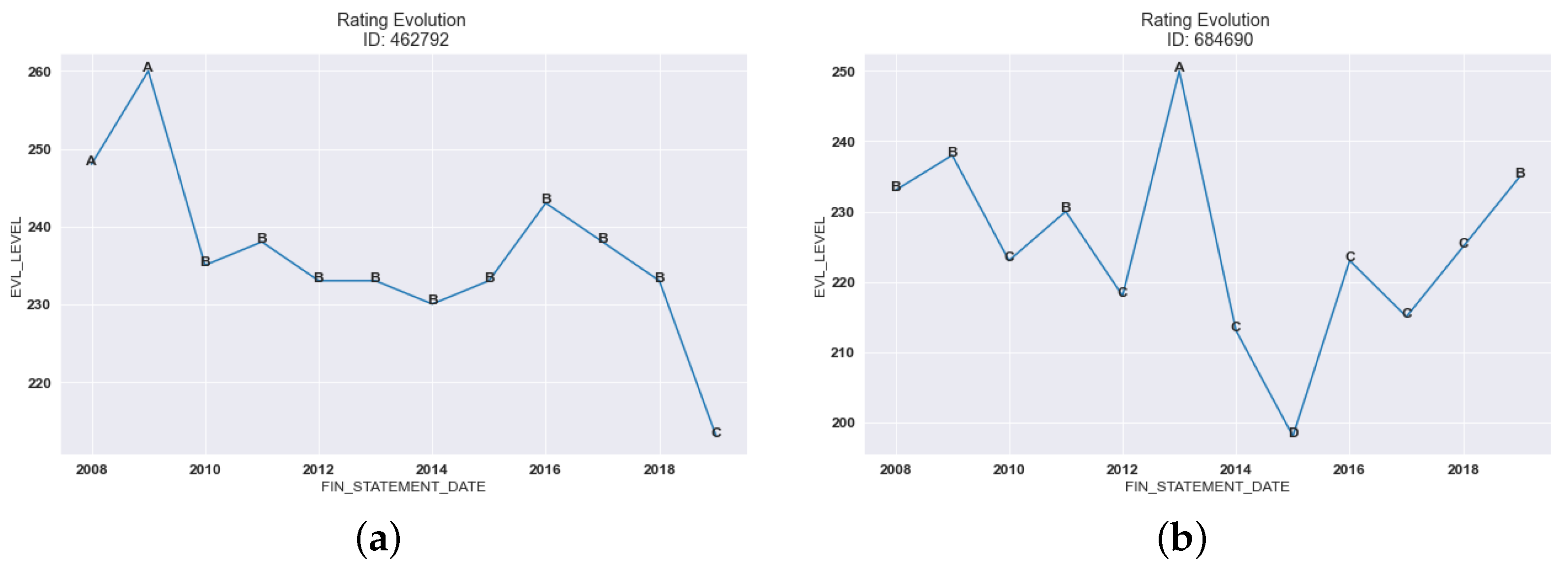
Time series dataset	3395

). Tinubu Square has an internal credit risk model that has been used for 20 years to assess the creditworthiness of a company (e.g., Figure 1). This internal model uses a large list of financial variables to compute a score. The score (i.e., EVL_LEVEL variable) is then mapped to a letter, which is the final result of Tinubu’s internal model. This rating represents the probability of default in a descriptive way. High-risk companies have lower scores and are represented with the rating letter F. On the other hand, companies whose PD is close to zero are represented with higher scores and have the rating letter A.

The purpose of this work was to create a forecasting model to predict the rating evolution of companies in Tinubu’s portfolio. In order to predict the future rating of a company, we needed to convert the original dataset into a time series dataset. Each row of this new dataset represented a company and the columns represented the year the company was rated.

3.2. Forecasting Time Series

In this part of the study we present the models proposed to address the problem of forecasting the creditworthiness of a company.

3.2.1. Autoregressive Moving Average Method

The autoregressive moving average (ARMA) method is a combination of two different models: an autoregressive model (AR) and a moving average model (MA). Mathematically, ARMA processes results from the sum of both processes: an AR of order p and an MA of order q. An ARMA(p, q) model combines both the AR(p) and MA(q) models as follows:

$$x_t=c+\sum _{i=1}^p{\varphi }_i{x}_{t-i}+{ϵ}_t+\sum _{i=1}^q{\theta }_i{ϵ}_{t-i}$$

(1)

The parameters p and q can be determined using different methods. By observing the graph of the autocorrelation function (ACF) and the partial autocorrelation function (PACF) both parameters can be estimated. In this work, we estimate the parameters using a more analytical approach by computing the Akaike information criterion (AIC) [17]. The AIC is a statistical measure that allows a comparison between statistical models to determine which model best fits the data series. The AIC considers both model goodness of fit and model complexity.

$$AIC=2k-2log\left(L\right)$$

(2)

where k is the number of parameters of the statistical model and L is the maximum value of the likelihood function for the model. The first term represents the complexity of the model, while the second term in Equation (2) represents how well the model fits the data.

3.2.2. Gradient Boosting

The extreme gradient boosting (XGBoost) software is a machine learning-based algorithm, consisting of a sequential combination of weak learners, that corrects the errors of the previous weak learner. XGBoost is an open-source framework proposed by [12] that has been widely used in machine learning competitions.

The outcome of an XGBoost composed of K weak learners for a dataset with n instances and m features $D=(x_i,y_i)\left(\right|D|=n,x_i\in {\mathbb{R}}^m,y_i\in \mathbb{R})$ is represented mathematically as follows:

$$\widehat{y_i}=\mathsf{\Omega }\left(X_i\right)=\sum _{k=1}^K{f}_k\left(X_i\right),f_k\in F$$

(3)

where $F=\{f\left(x\right)=w_{q\left(x\right)}\}(q:{\mathbb{R}}^m\to T,w\in {\mathbb{R}}^T)$ is the space regression of the trees. T is the number of leaves in the tree and q represents the structure of each tree that maps an example to the corresponding leaf index [12]. For each independent tree $f_k$ there is an independent q in addition to leaf weights $w_q$.

$$L^t=\sum _i\left(y_i,\widehat{y_i}\right)+\sum _k\mathsf{\Omega }\left(f_k\right)$$

(4)

where l is the loss function, $y_i$ is the target value, and ${\widehat{y}}_i$ is the prediction. The term $\mathsf{\Omega }$ penalizes the complexity of the function. This term was introduced to avoid overfitting.

For the hyperparameter estimation, we used scikit-learn [18] to perform a grid search, which consists of creating all possible hyperparameter combinations of a list of values predetermined by the user.

3.3. Comparing the Forecasted Values

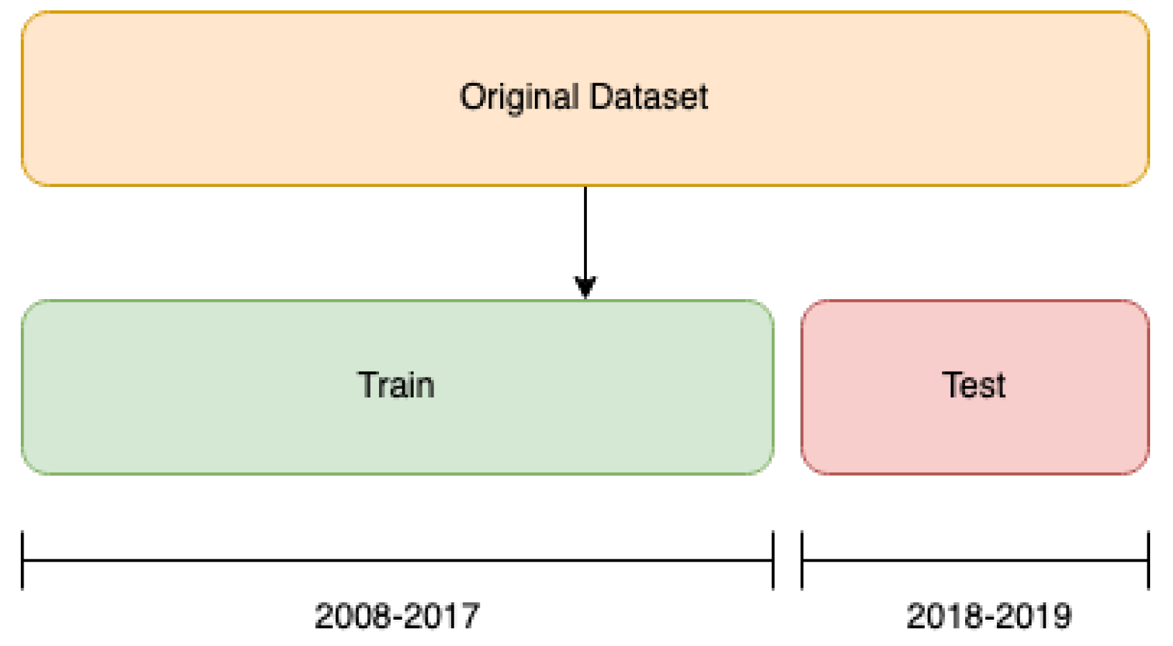
To assess the performance of both proposed models, we split the dataset into two different parts: the training set contained the score, and thus the rating, of companies during the period 2008–2017; the rest of the dataset, the test set, was composed of the rating of the same companies scored by Tinubu during the period 2018–2019 (see Figure 2).

We graphically compared the results of both models. For the ARMA model, we kept one ARMA from a company with hyperparameters p and q that minimized the AIC for the time series between the period 2008–2017. For each model we generated two predictions that corresponded to the years 2018 and 2019. We then compared the forecast of both models graphically.

4. Results

In this section we present the results of the models that were described in the previous section. First, we present the results of each model individually and then we compare the forecasted ratings for both models using several companies.

4.1. Assessing the Performance of the ARMA

As we mentioned previously, we created several ARMA models with different hyperparameters (i.e., p and q). For instance, we created nine different ARMA models and considered the best model the one with the lowest AIC. In

Table 2. For each company in the dataset, we created nine models. The best model was the one with the lowest AIC value. The AIC was computed over the training set, which consisted of companies rated every year by Tinubu Square during the period 2008–2017. We showed the difference between the predicted rating and the real rating. The values p and q are the hyperparameters of the ARMA model.

LGE_ID	2018	2019	Prediction 2018	Prediction 2019	p	q	AIC
462792	233 (B)	213 (C)	234 (B)	245 (B)	1	1	65.2517
462792	233 (B)	213 (C)	234 (B)	245 (B)	2	1	67.2505
462792	233 (B)	213 (C)	233 (B)	244 (B)	3	1	69.0822
462792	233 (B)	213 (C)	233 (B)	249 (A)	1	2	59.9773
462792	233 (B)	213 (C)	235 (B)	259 (A)	1	3	57.8751
462792	233 (B)	213 (C)	233 (B)	246 (B)	2	2	61.4822
462792	233 (B)	213 (C)	234 (B)	253 (A)	3	3	60.3457
462792	233 (B)	213 (C)	233 (B)	246 (B)	3	2	63.482
462792	233 (B)	213 (C)	236 (B)	253 (A)	2	3	58.4614

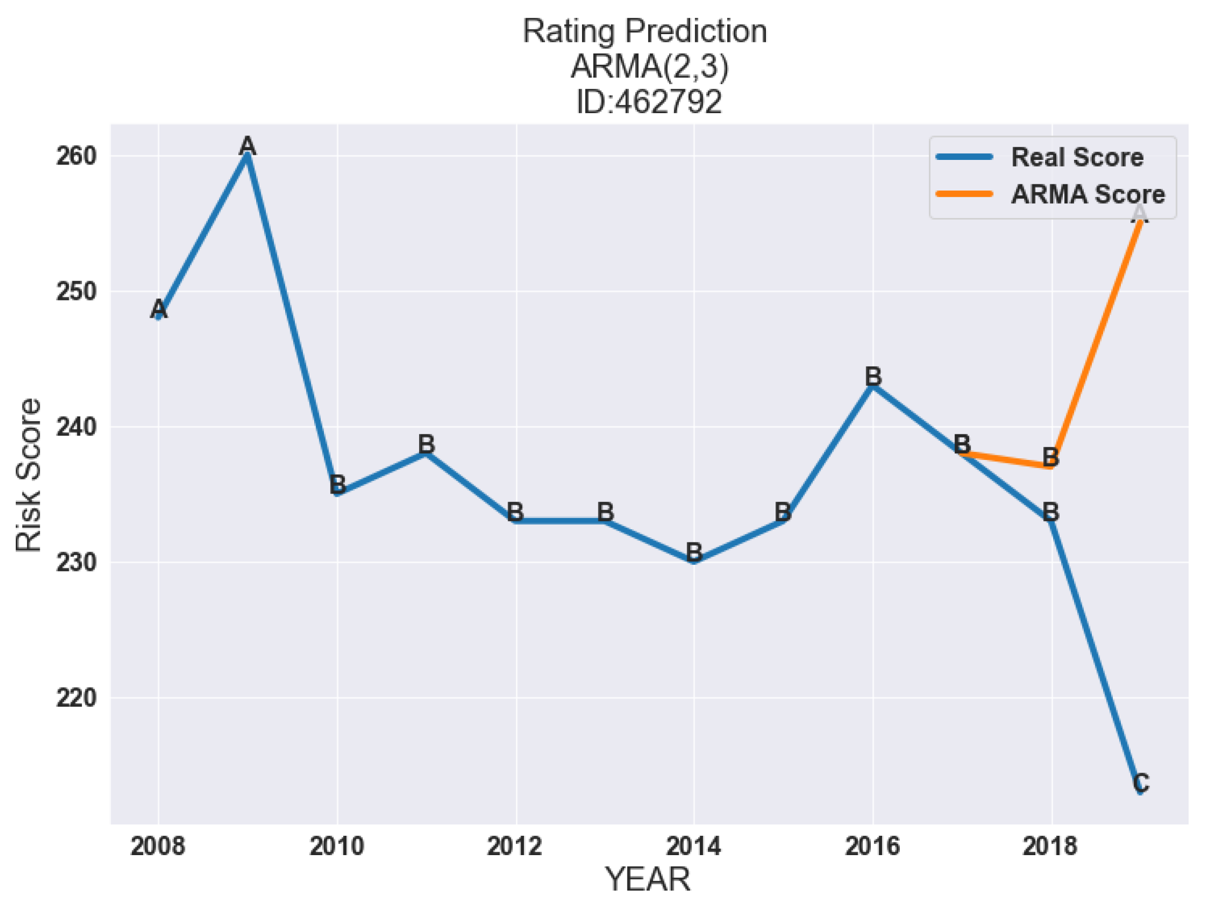
, the results obtained for the company with the id 462792 are shown. For this particular company, the hyperparameters with the lowest AIC were $p=2$ and $q=3$. When we forecast Tinubu’s score for the years 2018 and 2019 we observed that the model underestimated the risk, see Figure 3. The ARMA captured the smooth deterioration of the company for the year 2018. However, the difference between the model in 2019 was significant.

4.2. Forecasting Tinubu’s Score Using XGBoost

In this part of the study, we present the results obtained with XGBoost. In

Table 3. Optimal XGBoost hyperparameters found using grid search.

Hyperparameter	Value
n estimators	150
Learning rate	0.2
Max. depth	8

we show the optimal hyperparameters found using grid search optimization.

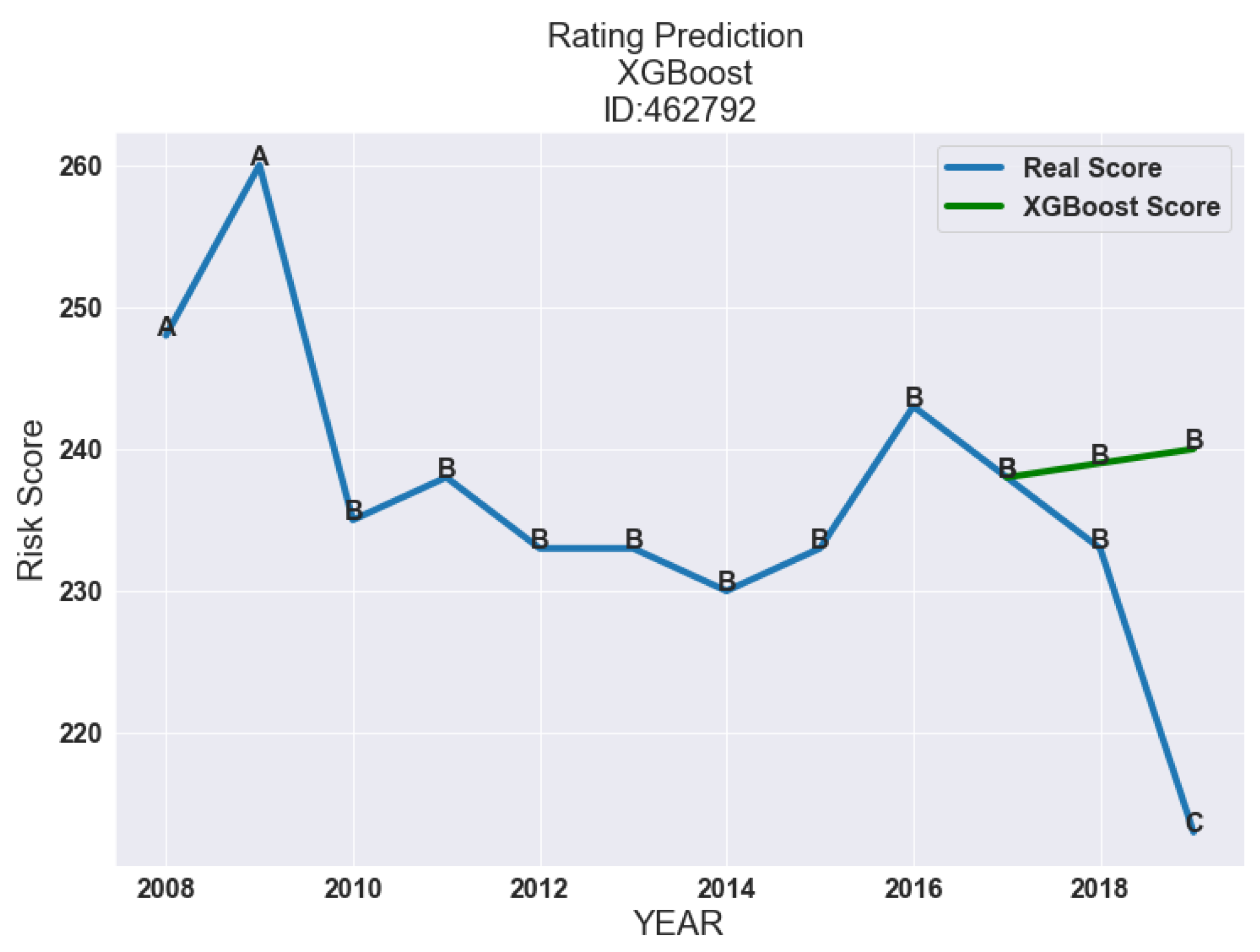
As we can see in Figure 4, the XGBoost showed that the company with the ID 462792 will slightly improve during the next two years. The rating given by Tinubu and the rating generated by our XGBoost model diverged for the year 2019. This difference can be explained by the fact there was an event that adversely affected the company’s activity.

4.3. Analyzing the Models’ Ratings

As we mentioned in previous sections, Tinubu’s rating system reflects the PD in a descriptive way. In this section, we present several examples of comparison between the behavior of both models for different companies with the rating given by Tinubu for the test period (see Figure 2).

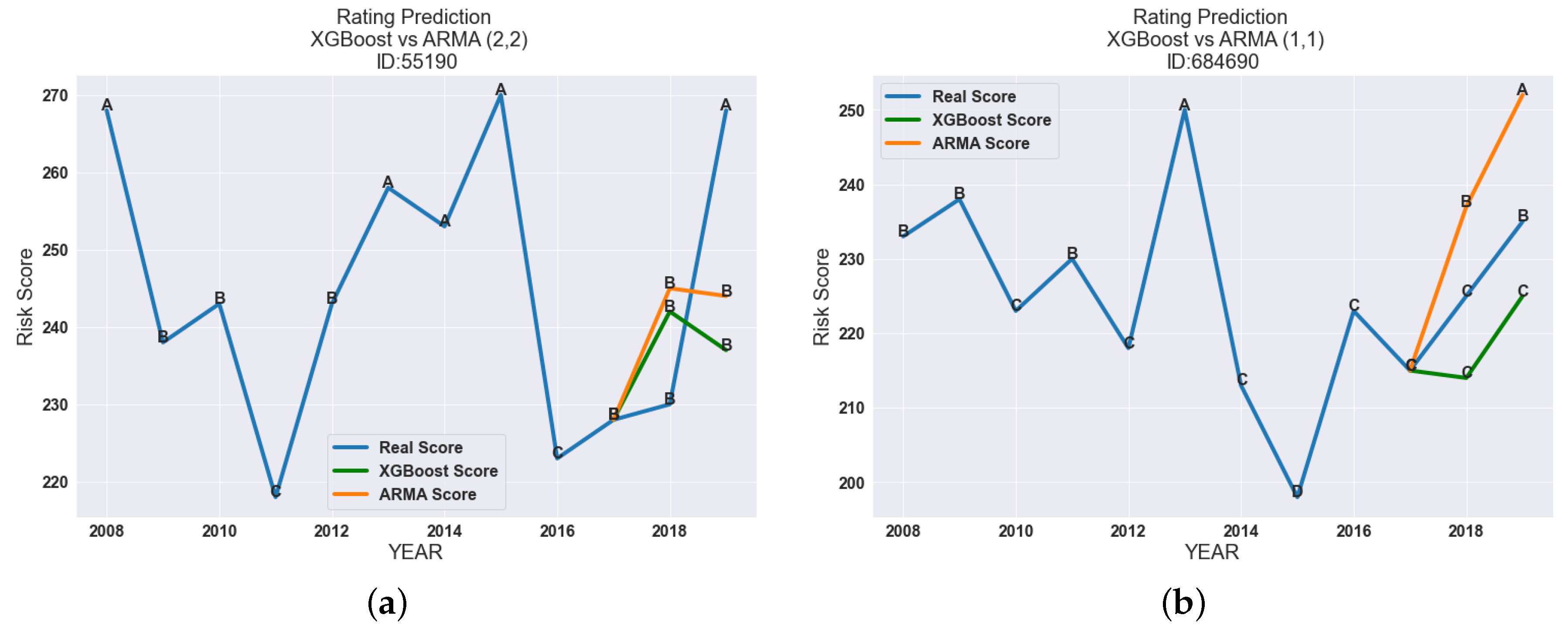
In Figure 5a, we compare the XGBoost with an ARMA with $p,q=2$. The results showed that, in this particular case, both models slightly underestimated the risk. On the other side, we observed that both models overestimated the risk.

For the company 684690 (see Figure 5b), the results showed a divergence between the ARMA model with $p,q=1$ and the XGBoost model. The latter could capture the evolution of the rating during the years 2018 and 2019 with a narrow difference between the predicted score and the score given by Tinubu. On the other side, the ARMA model, even if it captured the trend, clearly overestimated the company’s creditworthiness.

Nonetheless, there were cases where both models underestimated the risk. This is the case in Figure 6a. Both models assumed that the creditworthiness of the company for the next two years would have a downward trend.

Another relevant case is presented in Figure 7b. In this one, the ARMA with $p=1$, $q=3$ highly underestimated the risk by giving an A rating to a company for which Tinubu’s rating for the year 2019 was E.

5. Conclusions

In this work we proposed a framework for the credit scoring that differs from previous work in the field. The approach considered consisted of forecasting the credit rating of a large number of companies using an historic index given by Tinubu Square for the period 2008–2019. We used the period 2018–2019 to compare both forecasting models with the target value, which was Tinubu’s rating. We observed that for the set of companies analyzed, both models tended to slightly underestimate the risk. For companies specialized in credit risk, models that overestimate the risk are preferable to models that underestimate the risk. This is mainly because underestimating the risk can lead to potential economic losses. On the other hand, models that are strongly conservative (i.e., models that overestimate the risk) are not desirable for credit scoring since they impact the economic activity by reducing the volume of credits approved and thus decrease the business between SMEs. By considering this criteria and observing the results of our work we could conclude that the machine learning-based models are closer to Tinubu’s standards in terms of credit scoring. It is important to remark on the fact that wealthy companies (i.e., companies with rating classes in the range A–B) were more stable over the period analyzed than companies with a lower rating. Future work should focus on the adequate evaluation of the performance of the models proposed in this work. It will be interesting to introduce deep learning models and compare them with results yielded by the proposed models.

References

- Stability, F.; Services, F.; Union, C.M. Review of Country-by-Country Reporting Requirements for Extractive and Logging Industries; European Union: Geneva, Switzerland, 2018. [Google Scholar]
- Singleton-Green, B. SME Accounting Requirements: Basing Policy on Evidence. ICAEW. 2015. Available online: https://papers.ssrn.com/sol3/papers.cfm?abstract_id=2703246 (accessed on 9 September 2022).
- Florez-Lopez, R. Effects of missing data in credit risk scoring. A comparative analysis of methods to achieve robustness in the absence of sufficient data. J. Oper. Res. Soc. 2010, 61, 486–501. [Google Scholar] [CrossRef]
- Giudici, P.; Hadji-Misheva, B.; Spelta, A. Network Based Scoring Models to Improve Credit Risk Management in Peer to Peer Lending Platforms. Front. Artif. Intell. 2019, 2, 3. [Google Scholar] [CrossRef] [PubMed]
- Wang, Y.; Ni, X.S. Improving Investment Suggestions for Peer-to-Peer (P2P) Lending via Integrating Credit Scoring into Profit Scoring. In Proceedings of the 2020 ACM Southeast Conference, Tampa, FL, USA, 2–4 April 2020; pp. 141–148. [Google Scholar] [CrossRef]
- Provenzano, A.R.; Trifirò, D.; Jean, N.; Pera, G.L.; Spadaccino, M.; Massaron, L.; Nordio, C. An Artificial Intelligence approach to Shadow Rating. arXiv 2022, arXiv:1912.09764. [Google Scholar] [CrossRef]
- Qadi, A.E.; Trocan, M.; Díaz-Rodríguez, N.; Frossard, T. Feature contribution alignment with expert knowledge for artificial intelligence credit scoring. Signal Image Video Process. 2022. [Google Scholar] [CrossRef]
- Altman, E.I. Financial Ratios, Discriminant Analysis and the Prediction of Corporate Bankrupcy. J. Financ. 1968, 23, 589–609. [Google Scholar] [CrossRef]
- Memic, D. Assessing Credit Default using Logistic Regression and Multiple Discriminant Analysis:Empirical Evidence from Bosnia and Herzegovina. Interdiscip. Descr. Complex Syst. 2015, 13, 128–153. [Google Scholar] [CrossRef]
- Breiman, L. Random Forests. Mach. Learn. 2001, 45, 5–32. [Google Scholar] [CrossRef]
- Ke, G.; Meng, Q.; Finley, T.; Wang, T.; Chen, W.; Ma, W.; Ye, Q.; Liu, T. Lightgbm: A highly efficient gradient boosting decision tree. Adv. Neural Inf. Process. Syst. 2017, 30, 3146–3154. [Google Scholar]
- Chen, T.; Guestrin, C. XGBoost: A Scalable Tree Boosting System. In Proceedings of the 22nd ACM SIGKDD International Conference on Knowledge Discovery and Data Mining, San Francisco, CA, USA, 13–17 August 2016; pp. 785–794. [Google Scholar] [CrossRef]
- Baesens, B.; Gestel, T.V.; Viaene, S.; Stepanova, M.; Suykens, J.; Vanthienen, J. Benchmarking State-of-the-Art Classification Algorithms for Credit Scoring. J. Oper. Res. Soc. 2003, 54, 627–635. [Google Scholar] [CrossRef]
- Lessmann, S.; Baesens, B.; Seow, H.-V.; Thomas, L.C. Benchmarking state-of-the-art classification algorithms for credit scoring: An update of research. Eur. J. Oper. Res. 2015, 247, 124–136. [Google Scholar] [CrossRef]
- Niaki, S.T.A.; Hoseinzade, S. Forecasting S&P 500 index using artificial neural networks and design of experiments. J. Ind. Eng. Int. 2013, 9, 1. [Google Scholar] [CrossRef]
- Hiransha, M.; Gopalakrishnan, E.A.; Vijay, K.M.; Soman, K.P. NSE Stock Market Prediction Using Deep-Learning Models. Procedia Comput. Sci. 2018, 132, 1351–1362. [Google Scholar] [CrossRef]
- Akaike, H. A new look at the statistical model identification. IEEE Trans. Autom. Control. 1974, 19, 716–723. [Google Scholar] [CrossRef]
- Buitinck, L.; Louppe, G.; Blondel, M.; Pedregosa, F.; Mueller, A.; Grisel, O.; Niculae, V.; Prettenhofer, P.; Gramfort, A.; Grobler, J.; et al. API design for machine learning software: Experiences from the scikit-learn project. arXiv 2013, arXiv:1309.0238. [Google Scholar]