Proceeding Paper

Bayesian Surrogate Analysis and Uncertainty Propagation †

by
Sascha Ranftl
* and
Wolfgang von der Linden
Institute of Theoretical Physics-Computational Physics, Graz University of Technology, Petersgasse 16, 8010 Graz, Austria
*
Author to whom correspondence should be addressed.
Presented at the 40th International Workshop on Bayesian Inference and Maximum Entropy Methods in Science and Engineering, online, 4–9 July 2021.
Phys. Sci. Forum 2021, 3(1), 6; https://doi.org/10.3390/psf2021003006
Published: 13 November 2021

Abstract

:
The quantification of uncertainties of computer simulations due to input parameter uncertainties is paramount to assess a model’s credibility. For computationally expensive simulations, this is often feasible only via surrogate models that are learned from a small set of simulation samples. The surrogate models are commonly chosen and deemed trustworthy based on heuristic measures, and substituted for the simulation in order to approximately propagate the simulation input uncertainties to the simulation output. In the process, the contribution of the uncertainties of the surrogate itself to the simulation output uncertainties is usually neglected. In this work, we specifically address the case of doubtful surrogate trustworthiness, i.e., non-negligible surrogate uncertainties. We find that Bayesian probability theory yields a natural measure of surrogate trustworthiness, and that surrogate uncertainties can easily be included in simulation output uncertainties. For a Gaussian likelihood for the simulation data, with unknown surrogate variance and given a generalized linear surrogate model, the resulting formulas reduce to simple matrix multiplications. The framework contains Polynomial Chaos Expansions as a special case, and is easily extended to Gaussian Process Regression. Additionally, we show a simple way to implicitly include spatio-temporal correlations. Lastly, we demonstrate a numerical example where surrogate uncertainties are in part negligible and in part non-negligible.

1. Introduction

Uncertainty quantification of simulations has gained increasing attention, e.g., in the field of Computational Engineering, in order to address doubtful parameter choices and assess the models’ credibility. Surrogate models have become a popular tool to propagate simulation input uncertainties to the simulation output, particularly for modern day applications with high computational cost and many uncertain model parameters. For that, a parametrized surrogate model (synonyms: meta-model, emulator) is learned from a finite set of simulation samples. i.e., the surrogate is a function of the uncertain simulation input parameters that is ’fitted’ to the simulation output data. The quality of this fit is then judged by heuristic diagnostics, and the surrogate deemed trustworthy, respectively. A key aspect of this procedure is that the surrogate can be evaluated much faster than the simulation, and still retains a reasonable approximation to the simulation.
The simulation is then substituted with the surrogate model in order to compute the marginal probability density function of the simulation output. The simulation uncertainties are thus inferred from the surrogate model instead of the original simulation model at a significantly reduced computational effort. While this practice allows for obtaining estimates on uncertainties of expensive simulations in the first place, the contribution of the uncertainty of the surrogate itself to the total simulation uncertainty is commonly neglected. In other words, the estimation of the surrogate parameters based on the finite set of simulation samples entails an additional uncertainty in the sought-for uncertainty of the simulation output. The purpose of this paper is to investigate this surrogate uncertainty as the natural measure for the surrogate’s trustworthiness, and how the surrogate uncertainty affects the simulation output uncertainty.
In many cases, the surrogate uncertainty is indeed small if the heuristic diagnostics naively imply so. If the heuristic diagnostics imply that the surrogate is not trustworthy, one may resort to two options: (i) Acquire more simulation data until the surrogate is trustworthy. This is limited by the computational budget and the surrogate’s convergence properties. (ii) Shrink the parameter space, e.g., omit a number of uncertain simulation parameters by assuming definite parameter values. However, in some cases, (i) is not feasible and (ii) is not desired. In this contribution, we demonstrate how to include surrogate uncertainties if the user deals with a surrogate model with doubtful trustworthiness.
Popular surrogate models are Polynomial Chaos Expansions [1,2,3] and Gaussian Process Regression [4,5], the latter of which has had its renaissance recently from within the machine learning community. In this work, we assume a Gaussian likelihood for the simulation data with unknown variance and given a generalized linear surrogate model (i.e., linear in the surrogate parameters) that includes Polynomial Chaos Expansions as a special case and is easily extended to Gaussian Process Regression. Other Bayesian perspectives on Uncertainty Quantification of computer simulations with these popular surrogate models are given in [6,7,8,9,10,11,12,13]. A comprehensive collection of reviews on Uncertainty Quantification, from the point of view of computational engineering and applied mathematics, can be found in [14]. In [7,15], a statistician’s perspective is discussed. Here, we will use Bayesian Probability Theory [16].

2. Bayesian Uncertainty Quantification

We start with the general structure of uncertainty propagation problems based on surrogate models in Section 2.1. In Section 2.2, we analyze a generalized linear surrogate model with a Gaussian likelihood for the simulation data with unknown surrogate variance. In Section 2.3, we proceed to use the surrogate model to propagate the input uncertainties to the output, and show how the surrogate’s uncertainties too can be included.

2.1. General Structure of the Problem

The goal in this paper is to quantify the uncertainties of the simulation results for the observable z ( x ) at different measurement points x = 1 , . . . , N x in the simulation domain. e.g., z could be the mechanical stress resulting from a structural analysis with a finite element simulation, where x could denote the location of the measurement probe in or on the analyzed structure. z ( x ) depends on unknown or uncertain model parameters a = { a i } i = 1 N a , which are generally inferred from experimental data d exp . Based on these data, Bayes’ theorem allows for determining the posterior probability density function (pdf) for a ,
p a d exp , I ,
where all background information on the experiment is subsumed in I . The implications of the background information I will be discussed later. This pdf will be assumed to be (almost) arbitrary but given in the following considerations. It usually is the result of a statistical data analysis of the foregoing experiment. This experiment could be the measurement of some material property needed for the simulation, e.g., viscosity for a computational fluid dynamics simulation. The uncertainty of the model parameters a entails an uncertainty in the simulated observable z ( x ) , and the latter is determined by the marginalization rule,
p z ( x ) d exp , I = p z ( x ) a , d exp , I p a d exp , I d V a .
In the first pdf, we have struck out d exp because the knowledge of a suffices to perform the simulation to obtain z ( x ) . If a consists of only one or two parameters ( N a = 1 , 2 ), then the numerical evaluation of the integral over the model parameters a will typically require a few dozens to hundreds of simulations. The uncertainty propagation is then done and no surrogate is needed. However, this is the trivial case, and usually a will consist of way more parameters. Let us assume that a consists of, e.g., four parameters. That would imply the need for performing simulations at least 10 5 times, which is way too CPU expensive for most real problems. This can be avoided if the simulations are replaced by a surrogate model that approximates the observable z by a suitable parametrized surrogate function z sur = g ( a | c ) , where c are yet unknown parameters. The simulation may yield the observable z ( x ) at different sites x in the domain; however, x could also denote the time-instance in non-static problems. Clearly, the parameters of the surrogate model will also depend on those positions. Thus, we actually have
z ( x ) z sur ( x ) = g ( a | c ( x ) ) .
The unknown parameters will be inferred from a suitable training data. To this end, simulations are performed for a finite set of model parameters A s = { a s ( i ) } i = 1 N s and the corresponding observables Z s = { z s ( x ) , ( i ) } i , x = 1 N s , N x are computed and combined in D sim = { A s , Z s } . The surrogate parameters c ( x ) are then inferred from D sim , and the surrogate is thus constructed. We now proceed to substitute the simulation for the surrogate, z ( x ) z sur ( x ) , in order to solve Equation (2) at a significantly reduced computational cost. This implies that the background information has changed. We will denote this as I ˜ , suggesting that we take the observable z entering the integral in Equation (2) from the surrogate model Equation (3) rather than from the expensive simulation. More precisely, instead of Equation (2), we now need to consider
p z ( x ) d exp , D sim , I ˜ = d V a p z ( x ) a , D sim , d exp , I ˜ p a D sim , d exp , I ˜ .
As far as the (second) pdf for the model parameters is concerned, we can omit the information on the training set D sim , as it does not tell us anything about the model parameters. This pdf is actually the same as that in Equation (1), i.e., p a d exp , I ˜ = p a d exp , I , as it makes no difference for the model parameters how we solve the equations underlying the simulation. In the first pdf, we can omit the information on the experiment d exp , as we only need the simulation data D sim to fix the surrogate model, which in turn defines the observable z. The first pdf can be further specified by the marginalization rule upon introducing the surrogate parameters C = { c ( x ) } x = 1 N x , where x is an index denoting the measurement points as introduced for z ( x ) ,
p z ( x ) a , D sim , I ˜ = d V C p z ( x ) C , a , D sim , I ˜ p C a , D sim , I ˜ .
The first pdf is uniquely fixed by the knowledge of a and C , hence D sim is superfluous. Similarly, in the second pdf, where C is inferred from the training data, additional model parameters without the corresponding observables’ values z, are useless. In summary, substituting the latter equation into Equation (4), we have
p z ( x ) d exp , D sim , I ˜ = d V a d V C p z ( x ) C , a , I ˜ p C D sim , I ˜ p a d exp , I .
The first pdf is rather simple. According to the background information I ˜ , we will determine the observable via the surrogate model. Since the necessary parameters c ( x ) C and a are part of the conditional complex, the surrogate model allows only one value
z sur ( x ) = g ( a c ( x ) ) .
for the observable. This means that p z ( x ) C , a , I ˜ is equivalent to the probability density function for z ( x ) given z ( x ) = g ( a c ( x ) ) . Hence, the pdf is a Dirac-delta distribution
p z ( x ) C , a , I ˜ = δ z ( x ) g ( a c ( x ) ) .
Finally, we have
p z ( x ) d exp , D sim , I ˜ = d V a d V C δ z ( x ) g ( a c ( x ) ) p C D sim , I ˜ p a d exp , I .
Before we can evaluate this integral, we first need to determine the two terms, which have their own independent significance. The last term is the result of a data analysis of a specific foregoing experiment, and will therefore not be treated here. We will suppress the background information in the following, as ambiguities should no longer occur.

2.2. Bayesian Analysis and Selection of the Surrogate Model

We recall that Equation (7) allows for determining the pdf for the observable based on the pdf for the model parameters, and the pdf for the parameters of the surrogate model p C D sim that we will determine now. To this end, we have to specify the form of the surrogate model. We use the expansion
z sur = ν = 1 N p c ν Φ ν ( a ) ,
in terms of basis functions Φ ν ( a ) and expansion coefficients c ν . No further specification is needed at this point. Without loss of generality, we will use multi-variate Legendre polynomials for the numerical examples. This expansion is similar to the frequently used generalized Polynomial Chaos Expansfion [1], where the polynomials Φ ν ( a ) are orthogonal with respect to the L 2 inner product with the prior of a , p a , as an integration measure. However, here we actually consider a posterior p a d e x p that generally has no standard form, for which no standard orthogonal polynomial chaos basis is known, and for which conditional independence of the model parameters a does not hold. Polynomial Chaos Expansions have been extended to arbitrary probability measures [17] and dependent parameters [18], but, in the present context; however, these polynomials are not of primary interest and would only complicate the numerical evaluation. Note that the approach presented here does not demand any orthogonality properties for the basis, and thus avoid the practical problems encountered with the construction of such orthogonal bases. Parameters here may have complex dependence structures, and the only requirement for the probability distribution p a d exp is that the integrals with respect to it exist. As outlined in Section 2.1, N s simulations are performed for a set of model parameters A s = { a s ( i ) } i = 1 N s and the corresponding observables Z s are computed. The theory is so far agnostic to the experimental design of these simulations, and it is therefore not of concern here. Now, we want to determine the pdf for the surrogate parameters C , which are combined in a matrix with elements C ν , x , where ν enumerates the surrogate basis functions and x enumerates the measurement positions in the domain for which the observables are computed. We abbreviated the simulation data by the quantity D sim = { A s , Z s } , where the matrix Z s has the elements ( Z s ) i , x , which represent the observable z ( x ) at position x corresponding to the model parameter vector a s ( i ) . The sought-for pdf follows from Bayes’ theorem
p C D sim = p C Z s , A s p Z s C , A s p C A s p Z s C , A s .
The proportionality constant is not required in the ensuing considerations, and we have assumed an ignorant, uniform prior for the coefficients c , i.e., p C I = c o n s t . We note that this is also the transformation invariant Riemann prior (see Appendix B). However, any prior that is conjugate to the likelihood will retain analytical tractability. For the likelihood, we need the total misfit, which is given by
χ 2 = i = 1 N s x = 1 N x ( Z s ) i , x ν = 1 N p ( M s ) i , ν ( C ) ν , x 2 = i , x Z s M s C i , x 2 = tr Z s M s C T Z s M s C ,
with ( M s ) i , ν = Φ ν ( a s ( i ) ) and N s x = N s · N x . We assume a Gaussian type of likelihood, i.e.,
p Z s C , A s , Δ = Δ N s x Z exp χ 2 2 Δ 2 .
with normalization Z . We have mentioned the Δ -dependence of the normalization explicitly, while the rest of of the normalization is irrelevant in the present context. Usually, the misfit entering the likelihood comes from the noise of the data. In the present case, however, there is no noise (merely a tiny numerical error), but the surrogate model is presumably not an exact description of the simulation data and Δ covers the corresponding uncertainty. However, the uncertainty level Δ is not known and has to be marginalized over. Along with the appropriate Jeffreys’ prior, p C , Δ = p C p Δ , p Δ = 1 Δ , p C = c o n s t . (see Appendix B), the integration over Δ yields
p C Z s , A s = 1 Z χ 2 N s x 2 .
with terms independent of C subsumed in the normalization Z. For computing the mean, variance, and evidence, we first complete the square in Equation (9) to get a quadratic form in C , which can then be integrated analytically (see Appendix A). The result is
C a = H s 1 M s T Z s , H s = M s T M s ,
Δ C ν x Δ C ν x a = χ min 2 ( N s N p ) N x 2 H s 1 ν , ν δ x x , χ min 2 = tr Z s T 1 1 M s H s 1 M s T Z s .
We argue that the prefactor of H s 1 is the Bayesian estimate for Δ 2 , the variance of the Gaussian in Equation (10). This reasoning is similar to [19]. Note that Z s is a matrix of size N s × N x , containing the data vectors of length N s for each measurement site x. As shown in Appendix A, Equation (A6), the evidence for a particular set of surrogate models is computed as
p { z sur ( x ) } x = 1 N x D sim , I ˜ = Z = Ω N p x | H s | 1 2 χ min 2 N s x N p x 2 Γ ( N p x 2 ) Γ ( N s x N p x 2 ) Γ ( N s x 2 ) ,
where Ω N p x is the solid angle in N p x dimensions. The evidence is the probability for a surrogate model given the data. Note that this quantity does not depend on p a d exp , I . This is reasonable because the analysis of the experimental data should be independent of the analysis of the simulation data. However, p a d exp , I will typically be used for the experimental design of the simulation data acquisition. By comparing the evidence for different models, the user can choose a particular surrogate model or, if the results do not overwhelmingly suggest one single model, average the results for the surrogate analysis and the following uncertainty propagation over several plausible models. Note that the evidence is the pillar of a Bayesian procedure to select a surrogate model, and is distinct from the procedure of incorporating the trustworthiness or uncertainty of the surrogate in the subsequent uncertainty propagation.

2.3. Bayesian Uncertainty Propagation with Surrogate Models

Now that we have selected the surrogate model and determined the ingredients of Equation (7), we can determine the pdf for the observables in the light of the experimental data and the simulation results of the training set. The form in Equation (5) allows an easy evaluation of the mean value by using Equation (12) (see also Equation (A3)),
z ( x ) = d V a d V C f ( a c ( x ) ) p C D sim , I ˜ p a d exp , I = ν d V a Φ ν ( a ) C ν x a p a d exp , I .
Similarly, we obtain (see Equations (12) and (A8))
z ( x ) z ( x ) = d V a d V C f ( a c ( x ) ) f ( a c ( x ) ) p C D sim , I ˜ p a d exp , I = ν ν d V a Φ ν ( a ) Φ ν ( a ) C ν x C ν x a p a d exp , I = ν ν d V a Φ ν ( a ) Φ ν ( a ) C ν x a C ν x a + Δ C ν x Δ C ν x a p a d exp , I .
The covariance then follows from
Δ z ( x ) Δ z ( x ) = z ( x ) z ( x ) z ( x ) z ( x ) .
If we neglected the uncertainty of the surrogate, i.e.,
p C D s i m = δ ( C C ^ ) , C ^ = C a ,
then we retain the widely known special case of ’perfectly trustworthy’ surrogates
z ( x ) z ( x ) = ν ν d V a Φ ν ( a ) Φ ν ( a ) C ν x a C ν x a p a d exp , I .
Thus, the first part in the integral of Equation (15) is the uncertainty of the observable due to experimental uncertainties and given the surrogate model, while the second term adds the uncertainty of the surrogate itself. The term Δ C ν x Δ C ν x a is commonly neglected, but easily computed. This result also suggests a natural measure for the trustworthiness of the surrogate model, which is directly linked to the specific experiment:
ν ν d V a Φ ν ( a ) Φ ν ( a ) Δ C ν x Δ C ν x a p a d exp , I ν ν d V a Φ ν ( a ) Φ ν ( a ) C ν x a C ν x a p a d exp , I < ϵ .
If the surrogate uncertainties are, on average, smaller than the experimental uncertainties by a few orders of magnitude, e.g., ϵ = 10 3 , then they may be neglected. However, ϵ is the user’s choice. Note that this result does not spare the user to solve the foregoing surrogate model selection problem by e.g., computing evidence. This work only demonstrates how surrogate uncertainties can be incorporated and a practical rule when they could be neglected, given that the surrogate model has already been selected before.

3. Numerical Example

Here, we demonstrate an application where surrogate uncertainties were in part negligible and in part non-negligible. We apply our method to a computational fluid dynamics simulation of aortic hemodynamics, i.e., blood flow in an aorta resembled by the simplified geometry of an upside down umbrella stick. The simulation depends on a non-Newtonian viscosity model with four parameters a = { a 1 , a 2 , a 3 , a 4 } . The model was accompanied by viscosity measurements of human blood samples, thus determining p a d exp , I . This posterior turned out to have a complex landscape that cannot be reasonably approximated by standard distributions. Particularly, strong correlations and multi-modality were observed, i.e., p a d exp , I i p a i d exp , I . This means that vanilla Polynomial Chaos Expansions could not be applied without an undesirable transformation to conditionally independent variables. The posterior is described in detail in [20]. Based on p a d exp , I , N s = 100 parameter samples a s were chosen and the simulation evaluated accordingly. The output, Z s , was the absolute values of the wall shear stress that the blood flow exerts on the aortic wall, for N x = 10 measurement probes at different locations, each for N t = 101 time-instances equidistantly spaced over one cardiac cycle (ca. 1 s). Further details on the simulation are not relevant here but are documented [20]. A simulation time on the order of 150 CPU hours per sample suggested to use a surrogate for the inference. For the surrogate’s basis functions, Φ ν ( a ) , we found multi-variate Legendre polynomials of up to order two sufficient. The numerical integrals were computed with Riemannian quadrature and convergence checked with successive grid refinement; however, stochastic integration would work just as well. A sketch example on how to implement this procedure computationally efficient via vectorisation in parameter space can be found at https://github.com/Sranf/BayesianSurrogate_sketch.git (1 January 2021).
In Figure 1, we compare the simulation uncertainty (including surrogate uncertainty) as computed with our Bayesian approach (Equation (15)) to the naive estimate for the simulation uncertainty (without surrogate uncertainty, i.e., neglecting Δ C ν x Δ C ν x a in Equation (15). The surrogate uncertainties in the first half (left hand side) are relatively small, comprising only a few percent of the total uncertainty, and could possibly be neglected. In the second half (right-hand side), however, the surrogate uncertainties make up to ∼50% of the total uncertainty. This demonstrates that simulation uncertainties inferred via surrogate models can be severely underestimated if the surrogate uncertainties are neglected, and subsequently lead to overconfidence in the simulation model. In practice, one would acquire more data in order to reduce the surrogate uncertainties, e.g., more data at later time-instances in Figure 1 are particularly promising. This was limited here not only by the computational budget, but also the impracticality in that dynamic simulations require the full evaluation of all previous time instances where the surrogate is already reasonably accurate. Thus, the procedure of instead explicitly including the surrogate uncertainties here also has proven to be practical. A similar situation is to be expected for most transient simulations, as uncertainties will usually increase as time progresses.

4. Discussion

In this work, we have assumed a Gaussian likelihood for the simulation data, with unknown variance, for a surrogate that is linear in its parameters. Surrogates that are nonlinear in its parameters (e.g., neural networks) may promise higher capacity, however at the expense of losing analytical tractability of the surrogate uncertainty entirely. Other likelihood functions might be useful if further information is available, such as bounds on the observable (Gamma- or Beta-likelihood).
The result is a simple formula to incorporate surrogate uncertainties in the simulation uncertainties. This formula will be particularly useful if ’convergence’ in the sense of finding the coefficients of e.g., a Polynomial Chaos Expansion is doubtful or not achievable due to a limit to the computational budget. The formula immediately suggests an intrinsic measure for the trustworthiness of the surrogate, distinct from commonly used ad hoc diagnostics. This measure is not to be confused with the evidence and should not be used for model selection because it would not preclude over-fitting, etc. It is merely a measure for the trustworthiness of the already selected surrogate.
Let us now explore the connections of this work to Polynomial Chaos Expansions (PCE) and Gaussian Process Regression (GPR). PCE is a special case of our generalized linear surrogate model, in that the basis functions of the surrogate are chosen such that
Φ ν ( a ) Φ ν ( a ) p a d exp , I d V a : = δ ν , ν .
The double sum in Equation (15) then contracts to a single sum, and the diagonal of the term for the surrogate uncertainty, Δ C ν x Δ C ν x a , survives. This is expected, in that PCE is defined such that the basis functions are uncorrelated, but still the expansion coefficients must be uncertain to a finite degree, and this must carry over to the simulation uncertainty. A severe limitation of PCE is that it is rather difficult to find basis function sets { Φ ν } that fulfill Equation (18), depending on p a d exp , I . For most practical purposes, one demands (i) conditional independence of the simulation parameters, i.e., p a d exp , I = i p a i d exp , I , as well as (ii) simple standard distributions for p a i d exp , I , in order to find a solution (usually a tensor-product) to Equation (18). Known albeit tedious work-arounds are for (i) variable transformations and numerical orthonormalisation [18] and for (ii) PCE-constructions for arbitrary pdfs [17]. Note that also [17] demands (i) conditional independence of the simulation parameters. Note that our approach is not afflicted by above considerations, unless Equation (18) is specifically demanded. In the numerical example above, neither (i) nor (ii) were applicable. Finding a variable transformation in order to fulfill (i) or numerical construction of orthonormal basis functions can be difficult, and particularly inconvenient if sophisticated priors p a I are being used, e.g., Jeffreys’ generalized prior. An interesting alternative would be to model the input dependencies with vine copulas [21] in order to overcome the limitations of PCE addressed here. Unfortunately, no obvious vine copula was found for the example presented here.
Gaussian Process Regression would correspond to a change in the prior for z ( x ) in Equation (6) as follows:
p z ( x ) C , a , θ , I ˜ = N ( g ( a c ( x ) ) K ( θ ) .
where N denotes a normal distribution, and K is the prior’s covariance matrix and defined by the parametrized covariance function k, [ K ] i j = k ( a ( i ) , a ( j ) θ ) . This in turn would change ( Z s M s C ) T ( Z s M s C ) ( Z s M s C ) T K 1 ( Z s M s C ) in Equation (9). By again completing the square and following the same procedure, the corresponding results for mean Equation (12a), variance Equation (12b), and evidence Equation (13) are then retained by a simple substitution of
H s H ˜ s , H ˜ s = M s T K s 1 M s , χ m i n 2 χ ˜ m i n 2 , χ ˜ m i n 2 = tr Z s T ( K s 1 K s 1 M s H ˜ s M s T K s 1 ) Z s ,
where [ K s ] i j = k ( a s ( i ) , a s ( j ) θ ) is the likelihood’s covariance matrix evaluated at A s for the data set Z s at given θ . Equations (14) and (15) would preserve their form with the substitution
Φ ν ( a ) C a Φ ν ( a ) C a , θ + K * T K s 1 M s C a , θ , Δ C ν x Δ C ν x a Δ C ν x Δ C ν x a , θ K K * T K s 1 K * ,
where the subscript θ acknowledges that the right-hand side now depends on θ , and [ K * ] i j = k ( a ( i ) , a s ( j ) θ ) is the covariance between the training set A s and the ’test set’, i.e., the integration variable a . Note that the additionally introduced hyperparameters θ would require the choice of a prior for θ and marginalization wrt θ in Equation (7), and subsequently also Equations (12)–(15).
We now discuss the implications of I ˜ in contrast to the original background information I . I contains, most importantly, that the observable z is uniquely determined by the simulation for a given set of input parameters a . A prerequisite here was that the simulation is converged. For example, for finite element simulations, this would be a given mesh-converged spatial discretization. The proposition I ˜ additionally assumes Equations (3) and (6), so that it can be used to replace Equation (2) by Equation (4). Formally, this means, to get from Equations (2)–(4), we replace p ( z a , I ) p ( z a , c , I ˜ ) , where p ( z a , I ) = δ ( z z ( a ) ) , p ( z a , c , I ˜ ) = δ ( z z s u r ( a ) ) = δ ( z g ( a c ) ) . For example, I ˜ contains in comparison to I the additional assumption that we can use the value for z as predicted/approximated by the surrogate model. It also means that we introduce additional, artificial, and usually unknown regression parameters c that need to be marginalized over. The additional uncertainty introduced by this approximation (i.e., the surrogate assumption) is encoded in p ( c | D sim , I ˜ ) , and is correctly incorporated into the simulation observable uncertainties in Equation (15). What is important here is that p ( z d exp , D sim , I ˜ ) p ( z d exp , D sim , I ) in general (the latter is computationally infeasible), but p ( z d exp , D sim , I ˜ ) p ( z d exp , D sim , I ) if Equation (3) holds and p ( C D sim ) δ ( C C ^ ) , i.e., if the surrogate is indeed a good approximation and the posterior for the surrogate parameters is sharply peaked at C ^ . Very often, this posterior is not sharply peaked; then, we can just gather more data until it is, or, if that is not possible, we can at least avoid overconfidence induced by neglecting these uncertainties. A numerical example of where this is the case has been demonstrated above.
We have modeled spatial correlations by introducing a location index x, and assumed that the expansion coefficients at different sites, c ( x ) and c ( x ) , are conditionally independent. This assumption is reasonable, in that the expansion coefficients are arbitrary mathematical constructs and no physically motivated model for their correlation is known. The spatial correlation, however, is retained in z ( x ) , as was originally intended. More general models for spatial correlations can easily be implemented by substitution of δ x x with a spatial covariance matrix in Equation (12b). Note that this would require an additional marginalization wrt the (typically nonlinear) hyperparameters of the spatial covariance matrix. By introducing a compound index x ˜ = ( x , t ) and substituting x x ˜ , we find a simple generalization to spatio-temporal correlations. This is equivalent to re-ordering spatial and temporal indices into a single sequence. While this procedure is convenient and requires only minor changes in the numerical implementation, it implicitly assumes conditional independence of spatial and temporal correlations. Analogous to above, general temporal correlations can be modeled by a substitution of δ x ˜ x ˜ in Equation (12b) with a temporal covariance matrix, again requiring an additional marginalization wrt the latter’s hyperparameters.

5. Conclusions

We presented a Bayesian analysis of surrogate models and its associated uncertainty propagation problem in the context of uncertainty quantification of computer simulations. The assumptions were a generalized linear surrogate model (linear in its parameters, not the variable) and a Gaussian likelihood with unknown variance. Additionally, spatial and temporal correlations have been discussed. The result suggests a measure of trustworthiness of the surrogate by quantifying the ratio of the surrogate uncertainty to the total uncertainty, in contrast to commonly used heuristic diagnostics. The main result, however, is a rather simple rule to include surrogate uncertainties in the sought-for uncertainties of the simulation output. This is useful particularly for problems where the surrogate’s trustworthiness is doubtful and cannot be improved. The connections to Polynomial Chaos Expansions and Gaussian Process Regression have been discussed. A numerical example demonstrated that simulation uncertainties can be significantly underestimated if surrogate uncertainties are neglected.

Funding

This work was funded by Graz University of Technology (TUG) through the LEAD Project “Mechanics, Modeling, and Simulation of Aortic Dissection” (biomechaorta.tugraz.at) and supported by GCCE: Graz Center of Computational Engineering.

Data Availability Statement

All information is contained in the manuscript. Code sketches are available at https://github.com/Sranf/BayesianSurrogate_sketch.git (1 January 2021).

Acknowledgments

The authors are grateful for useful comments from Ali Mohammad-Djafari.

Conflicts of Interest

The authors declare no conflict of interest.

Appendix A. Mathematical Proofs

Here, we want to determine norm, mean, and covariance of the marginalized Gaussian (Student-t distribution) in Equation (11), which is
p C Z s , A s = 1 Z χ 2 N s x 2 , χ 2 = tr Z s M s C T Z s M s C .
In order to perform the integration, we first complete the square to get a quadratic form in C , which can then be integrated analytically, i.e., we bring the misfit χ 2 into a form that elucidates the C -dependence
χ 2 = χ min 2 + tr C C ^ T H s C C ^ , H s = M s T M s , χ min 2 = tr Z s T 1 1 M s H s 1 M s T Z s , C ^ = H s 1 M s T Z s .
Now, the first moment is easily obtained. Along with the variable transformation under the integral
C C ^ + X
we obtain
C = 1 Z d V C C tr ( C C ^ ) T H s ( C C ^ ) + χ min 2 N s x 2 = C ^ + 1 Z d V X X X T H s X + χ min 2 N s x 2 = 0 .
where we have used the symmetry properties of the likelihood. Next, we transform the expression for normalization based on Equation (A3)
Z N s x = d V X tr X T H s X + χ min 2 N s x 2 .
Now, we combine and reorder the double indices ( ν , x ) into a single index l, which turns the matrix X of dimension N p × N x into a vector x of dimension N p x = N p · N x and the matrix H of dimension N p × N p into a new block matrix H of dimension N p x × N s x such that
[ H ] l l = [ H s ] ν , ν δ x x .
In this representation, we have
Z N s x = d V x x T H x + χ min 2 N s x 2 = | H | 1 2 d V y y T y + χ min 2 N s x 2 ,
where we substituted x H 1 2 y . Next, we introduce hyper-spherical coordinates, which leads to
Z N s x = Ω N p x | H | 1 2 0 d ρ ρ ρ N p x ( ρ 2 + χ min 2 ) N s x 2 ,
where Ω N p x is the solid angle in N p x dimensions. Finally, based on the substitution ρ = t · χ min 2 , we recover an identity of the Beta-function, and we obtain
Z N s x = Ω N p x | H | 1 2 χ min 2 N s x N p x 2 Γ ( N p x 2 ) Γ ( N s x N p x 2 ) Γ ( N s x 2 ) .
This result is valid only for N s x > N p x , which is fulfilled in the present application. For future use, we rewrite this as
Z N s x = Z ( N s x 2 ) · χ min 2 1 · N s x N p x 2 N s x 2 .
Finally, we calculate the covariance, based also on the compound index l = ( ν , x ) , and by using the variable transformation in Equation (A2):
Δ C l Δ C l = 1 Z N s x d V x x l x l x T H x + χ min 2 N s x 2 , = 2 N s x 2 · 1 Z N s x · H l , l d V x x T H x + χ min 2 N s x 2 + 1 , = 2 N s x 2 χ min 2 · ( N s x 2 ) Z ( N s x 2 ) · ( N s x N p x 2 ) H l l Z ( N s x 2 ) , = 2 χ min 2 ( N s x N p x 2 ) H l l ln ( Z ( N s x 2 ) ) , = 2 χ min 2 ( N s x N p x 2 ) H l l ln ( | H | 1 2 ) = 1 2 H 1 l l .
In the last step, we have used that H is a symmetric matrix. This is a very reasonable result because, if the variance Δ 2 in the Gaussian in Equation (10) would be known, then the covariance is Δ 2 H 1 . Consequently, the prefactor represents the Bayesian estimate for the variance Δ 2 based on the data. Now, we go back to the original meaning of the compound index Equation (A4), i.e., H 1 l l ( H s 1 ) ν ν δ x x , and obtain the final result.

Appendix B. The Transformation Invariant Prior for the Surrogate Coefficients

Bayesian probability theory allows for rigorously and consistently incorporating any prior knowledge we have about the experiment before taking a look at the data. This knowledge shall be elicited here. Our inference must not depend on the exact parametrization. e.g., if we re-parametrize the surrogate, re-label, or re-order the surrogate parameters, the surrogate still should describe the same simulation. This is reasonable because the surrogate is a purely mathematical, auxiliary construct. This rescaling-invariance is ensured by Jeffreys’ generalized prior and is given by the Riemann metric R (or the determinant of the Fisher information matrix) [16]
p ( C ) = 1 Z | det ( R ) | 1 / 2 with R i j = p Z s C 2 C i C j ln p Z s C d V Z s .
with multi-indices i , j = ( ν , x ) . With the likelihood and the generalized surrogate model defined in the manuscript, the result is
R i j k = 1 N s g ( a s ( k ) C ) C i g ( a s ( k ) C ) C j = k = 1 N s Φ i ( a s ( k ) ) Φ j ( a s ( k ) ) = c o n s t .
This prior is independent of C , i.e., a constant.

References

  1. Xiu, D.; Karniadakis, G.E. The Wiener-Askey polynomial chaos for stochastic differential equations. SIAM J. Sci. Comput. 2005, 27, 1118–1139. [Google Scholar] [CrossRef]
  2. O’Hagan, A. Polynomial Chaos: A Tutorial and Critique from a Statistician’s Perspective. 2013. Available online: http://tonyohagan.co.uk/academic/pdf/Polynomial-chaos.pdf (accessed on 25 June 2019).
  3. Crestaux, T.; Le Maître, O.P.; Martinez, J.-M. Polynomial chaos expansion for sensitivity analysis. Reliab. Eng. Syst. Saf. 2009, 94, 1161–1172. [Google Scholar] [CrossRef]
  4. O’Hagan, A. Curve Fitting and Optimal Design for Prediction. J. R. Stat. Soc. Ser. B 1978, 40, 1–42. [Google Scholar] [CrossRef]
  5. Rasmussen, C.E.; Williams, C.K. Gaussian Processes for Machine Learning; The MIT Press: Cambridge, MA, USA, 2006. [Google Scholar]
  6. Sraj, I.; Le Maître, O.P.; Knio, O.M.; Hoteit, I. Coordinate transformation and Polynomial Chaos for the Bayesian inference of a Gaussian process with parametrized prior covariance function. Comput. Methods Appl. Mech. Eng. 2016, 298, 205–228. [Google Scholar] [CrossRef] [Green Version]
  7. O’Hagan, A.; Kennedy, M.C.; Oakley, J.E. Uncertainty analysis and other inference tools for complex computer codes. Bayesian Stat. 1999, 6, 503–524. [Google Scholar]
  8. Kennedy, M.C.; O’Hagan, A. Predicting the output from a complex computer code when fast approximations are available. Biometrika 2000, 87, 1–13. [Google Scholar] [CrossRef] [Green Version]
  9. Arnst, M.; Ghanem, R.G.; Soize, C. Identification of Bayesian posteriors for coefficients of chaos expansions. J. Comput. Phys. 2010, 229, 3134–3154. [Google Scholar] [CrossRef] [Green Version]
  10. Madankan, R.; Singla, P.; Singh, T.; Scott, P.D. Polynomial-chaos-based Bayesian approach for state and parameter estimations. J. Guid. Control Dyn. 2013, 36, 1058–1074. [Google Scholar] [CrossRef] [Green Version]
  11. Karagiannis, G.; Lin, G. Selection of polynomial chaos bases via Bayesian model uncertainty methods with applications to sparse approximation of PDEs with stochastic inputs. J. Comput. Phys. 2014, 259, 114–134. [Google Scholar] [CrossRef] [Green Version]
  12. Lu, F.; Morzfeld, M.; Tu, X.; Chorin, A.J. Limitations of polynomial chaos expansions in the Bayesian solution of inverse problems. J. Comput. Phys. 2015, 282, 138–147. [Google Scholar] [CrossRef] [Green Version]
  13. Hwai, M.; Tan, Y. Sequential Bayesian Polynomial Chaos Model Selection for Estimation of Sensitivity Indices. SIAM/ASA J. Uncertain. Quantif. 2015, 3, 146–168. [Google Scholar] [CrossRef]
  14. Ghanem, R.G.; Owhadi, H.; Higdon, D. Handbook of Uncertainty Quantification; Springer: New York, NY, USA, 2017. [Google Scholar] [CrossRef]
  15. O’Hagan, A. Bayesian analysis of computer code outputs: A tutorial. Reliab. Eng. Syst. Saf. 2006, 91, 1290–1300. [Google Scholar] [CrossRef]
  16. von der Linden, W.; Dose, V.; von Toussaint, U. Bayesian Probability Theory: Applications in the Physical Sciences, 1st ed.; Cambridge University Press: Cambridge, UK, 2014. [Google Scholar] [CrossRef]
  17. Oladyshkin, S.; Nowak, W. Data-driven uncertainty quantification using the arbitrary polynomial chaos expansion. Reliab. Eng. Syst. Saf. 2012, 106, 179–190. [Google Scholar] [CrossRef]
  18. Jakeman, J.D.; Franzelin, F.; Narayan, A.; Eldred, M.; Plfüger, D. Polynomial chaos expansions for dependent random variables. Comput. Methods Appl. Mech. Eng. 2019, 351, 643–666. [Google Scholar] [CrossRef] [Green Version]
  19. von der Linden, W.; Preuss, R.; Hanke, W. Consistent Application of Maximum Entropy to Quantum-Monte-Carlo Data. J. Physics: Condens. Matter 1996, 8, 1–13. [Google Scholar] [CrossRef]
  20. Ranftl, S.; Müller, T.; Windberger, U.; von der Linden, W.; Brenn, G. Data and Codes for ’A Bayesian Approach to Blood Rheological Uncertainties in Aortic Hemodynamcis’; Zenodo Digital Repository: Genève, Switzerland, 2021. [Google Scholar] [CrossRef]
  21. Torre, E.; Marelli, S.; Embrechts, P.; Sudret, B. A general framework for data-driven uncertainty quantification under complex input dependencies using vine copulas. Probabilistic Eng. Mech. 2019, 55, 1–16. [Google Scholar] [CrossRef] [Green Version]
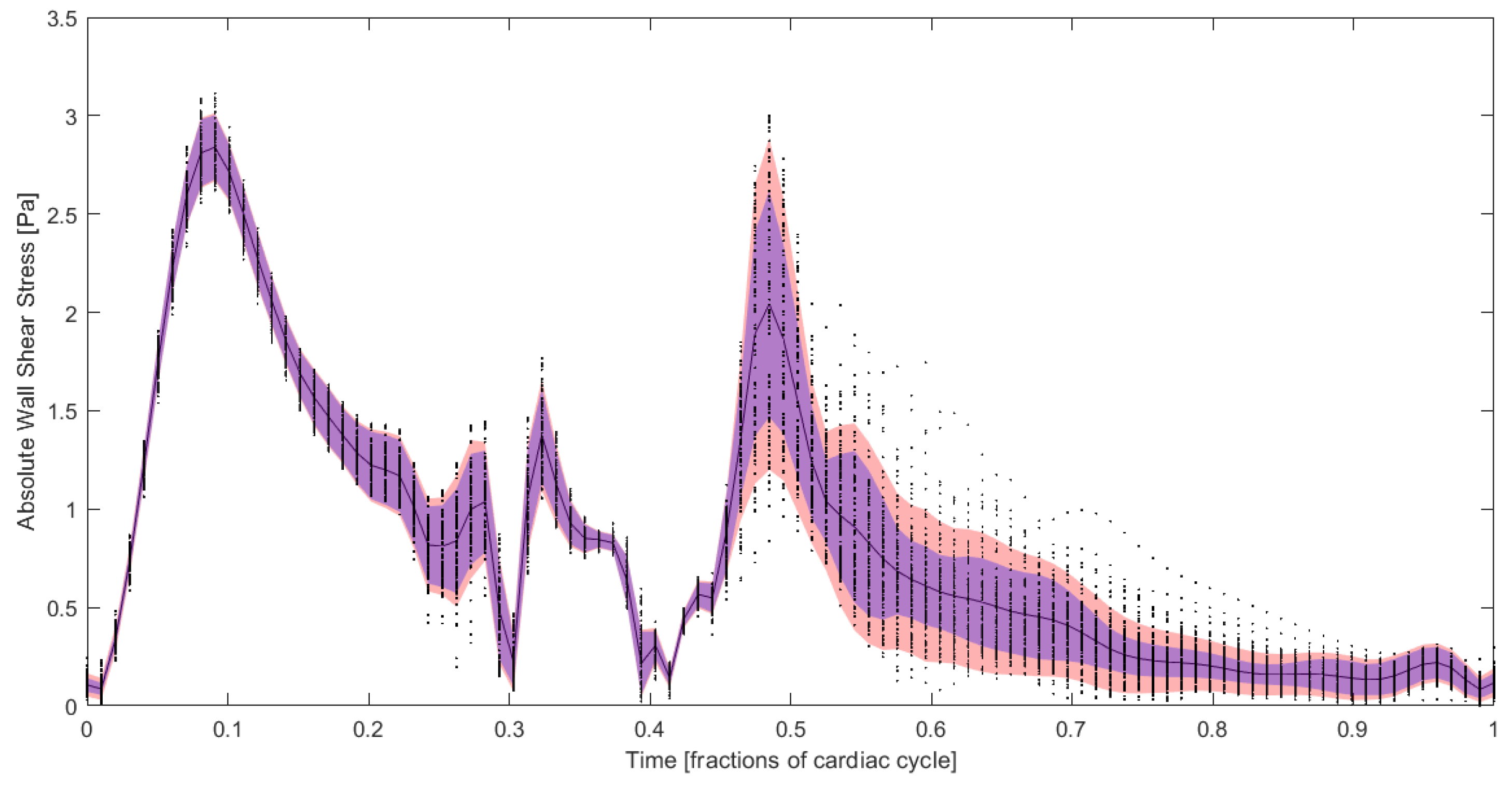
Figure 1. Simulation data (black dots) and simulation uncertainty ( 1 σ ) according to our Bayesian approach (red, including surrogate uncertainty) as well as the naive simulation uncertainty (blue, neglecting surrogate uncertainty). The black line is the surrogate mean.
Psf 03 00006 g001
Publisher’s Note: MDPI stays neutral with regard to jurisdictional claims in published maps and institutional affiliations.