Global Variance as a Utility Function in Bayesian Optimization ^†

Abstract

A Gaussian-process surrogate model based on already acquired data is employed to approximate an unknown target surface. In order to optimally locate the next function evaluations in parameter space a whole variety of utility functions are at one’s disposal. However, good choice of a specific utility or a certain combination of them prepares the fastest way to determine a best surrogate surface or its extremum for lowest amount of additional data possible. In this paper, we propose to consider the global (integrated) variance as an utility function, i.e., to integrate the variance of the surrogate over a finite volume in parameter space. It turns out that this utility not only complements the tool set for fine tuning investigations in a region of interest but expedites the optimization procedure in toto.

1. Introduction

In many experimental or theoretical approaches the effort of acquiring data may be costly, time consuming or both. The goal is to get insights in either the overall or extremal behaviour of a target quantity with respect to a set of parameters. If insights to functional dependencies between target and parameters are only to be obtained from a computationally expensive function, which may be considered as a black box function, it is instructive to employ surrogate modelling: already acquired data serve as a starting basis for establishing a surrogate surface in parameter space which then gets explored by Bayesian optimization [1]. An overall survey about Bayesian optimization may be found in [2], though it concentrates on an expected improvement (EI) utility and considers noise in the data only in the last paragraph, again by concentrating on EI. In contrast to this nice study we propose to alternate the different utilities at hand. Moreover, a fast information theory related to Bayesian optimization is shown in [3], though this approach approximates any black-box function by a parabolic form which differs from our ansatz letting the black-box function untouched. Interesting insights to multi-objective Bayesian optimization are provided by [4], which considers “multi-objective” in the sense of seeking the extrema–each is free of choice maximum or minimum–of a bunch of single-objective functions. However, the present paper concentrates on finding a common extremum depending on multiple parameters.

For the surrogate modelling we use the Gaussian process method (GP) [5] whose early stages date back to the middle of last century with very first efforts in geosciences [6] tackling the problem of surrogate modelling by so-called kriging [7]. Afterwards, GP has been appreciated much in the fields of neural networks and machine learning [8,9,10,11,12] and further work showed the applicability of active data selection via variance based criterions [13,14]. Our implementation of the GP method in this paper was already introduced at [15], and follows in notation–and apart from small amendments—the very instructive book of Rasmussen & Williams [5].

While in a previous work [16] we investigated the performance of utility functions for the expected improvement of an additional data point or for a data point with the maximal variance, in this paper we would like to introduce the global variance, i.e., the integral over the variance for a target surrogate within a region of interest with respect to a newly added data point. It is the substantial advantage of the Gaussian process method that such a task may be tackled simply on the basis of already acquired data, i.e., before new data have to be determined.

2. Global Variance for Gaussian Process-Based Model

In the following we concisely report the formulas leading to the results in this paper. For a thorough discussion of Gaussian processes please refer to the above mentioned papers, especially to the book of Rasmussen & Williams [5].

The problem of predicting function values in a multi-dimensional space supported by given data is a regression problem for a non-trivial function of unknown shape. Given are n target data $\mathit{y}$ for input data vectors ${\mathit{x}}_i$ of dimension $N_{\dim }$ with matrix $\mathit{X}$ = $({\mathit{x}}_1,{\mathit{x}}_2,\dots ,{\mathit{x}}_n)$ written as

$$\mathit{y}=\left(\begin{array}{c}{y}_1\\ y_2\\ ⋮\\ y_n\end{array}\right),{\mathit{x}}_i=\left(\begin{array}{c}{x}_{i1}\hfill \\ x_{i2}\hfill \\ ⋮\hfill \\ x_{i{N}_{\dim }}\hfill \end{array}\right),\mathit{X}=\left(\begin{array}{cccc}{x}_{11}\hfill & x_{21}\hfill & \cdots \hfill & x_{n1}\hfill \\ x_{12}\hfill & x_{22}\hfill & \cdots \hfill & x_{n2}\hfill \\ ⋮\hfill & ⋮\hfill & \ddots \hfill & ⋮\hfill \\ x_{1N_{\dim }}\hfill & x_{2N_{\dim }}\hfill & \cdots \hfill & x_{n{N}_{\dim }}\hfill \end{array}\right).$$

(1)

We assume that target data $y_i$ are blurred by Gaussian noise with ${\sigma }_{d_i}^2$. Further, we assume that the black box function interconnecting input $\mathit{X}$ and target $\mathit{y}$ is at least uniformly continuous and thereby justifies a description of a target surface with a surrogate from the Gaussian process method. Despite the experimental data and the physics background all quantities throughout this paper are without units.

The decisive quantity of a Gaussian process is the covariance function k describing the distance between two vectors $x_p$ and $x_q$ defined by

$$k(x_p,x_q)={\sigma }_f^{2}exp\left\{-\frac{1}{2}{\left|\frac{x_p-x_q}{\lambda }\right|}^2\right\}.$$

(2)

with the signal variance ${\sigma }_f^2$ and length scale $\lambda$. A covariance matrix ${\left(\mathit{K}\right)}_{ij}=k({\mathit{x}}_i,{\mathit{x}}_j)$ considers the covariances of all input data $\mathit{X}$. The GP method describes a target value $f_{*}$ at test input vector ${\mathit{x}}_{*}$ by a normal distribution $p\left(f_{*}\right|\mathit{X},\mathit{y},{\mathit{x}}_{*})\propto \mathcal{N}\left({\overline{f}}_{*},\mathrm{var}\left(x_{*}\right)\right)$ with mean ${\overline{f}}_{*}={\mathit{k}}_{*}^T{\left(\mathit{K}+{\sigma }_n^2\Delta \right)}^{-1}y$, and variance $\mathrm{var}\left({\mathit{x}}_{*}\right)=\mathit{k}({\mathit{x}}_{*},{\mathit{x}}_{*})-{\mathit{k}}_{*}^T{\left(\mathit{K}+{\sigma }_n^2\Delta \right)}^{-1}{\mathit{k}}_{*}$, where the term ${\sigma }_n^2\Delta$ represents the degree of information in the data. While $\Delta$ is the diagonal matrix of the given variances ${\sigma }_{d_i}^2$, the variance ${\sigma }_n^2$ accounts for an overall noise in the data. Then the full covariance matrix $\mathit{M}$ of the Gaussian Process is

$$\mathit{M}=\mathit{K}+{\sigma }_n^2\Delta$$

(3)

In Bayesian probability theory the three parameters $\mathbf{\theta }={(\lambda ,{\sigma }_f,{\sigma }_n)}^T$ are considered to be hyper-parameters which show up in the marginal likelihood as

$$logp\left(\mathit{y}\right|\mathbf{\theta })=\mathrm{const}-\frac{1}{2}{\mathit{y}}^T{\left[\mathit{K}(\lambda ,{\sigma }_f)+{\sigma }_n^2\Delta \right]}^{-1}\mathit{y}-\frac{1}{2}log\left|\mathit{K}(\lambda ,{\sigma }_f)+{\sigma }_n^2\Delta \right|.$$

(4)

In [16], we showed, that for a sufficiently large data base the target surrogate is well described by using the expectation values of the hyper-parameters in the formulas for $f_{*}$ and $\mathrm{var}\left(f_{*}\right)$, at least well enough to determine a global optimum in a region of interest (RoI). The global optimum is found by employing utility functions, as there are the expected improvement $U_{\mathrm{EI}}\left({\mathit{x}}_{*}\right)=\langle I\rangle ={\int }_{f_{\max }}^{\infty }{f}_{*}p\left(f_{*}\right|\mathit{X},\mathit{y},{\mathit{x}}_{*})\mathrm{d}{f}_{*}$ and the maximum variance $U_{\mathrm{MV}}\left({\mathit{x}}_{*}\right)=\mathrm{var}\left(f_{*}\right)$. For both the respective maximum at ${{\mathit{x}}_{*}}_{\max }=arg{max}_{\left\{{\mathit{x}}_{*}\right\}}{U}_{\mathrm{EI}/\mathrm{MV}}$ is sought. While the first one ($U_{\mathrm{EI}}$) evaluates the possible information gain from a new data point, the second utility ($U_{\mathrm{MV}})$ simply estimates the vector in input space with largest variance in the target surrogate.

In order to have a look on the implications of an additional data point in the surrogate, we propose a further utility function, i.e., the global variance defined on the multi-dimensional RoI$\in [-\mathbf{1}:\mathbf{1}]$ by

$$U_{\mathrm{GV}}={\int }_{-\mathbf{1}}^{\mathbf{1}}\mathrm{var}\left(\mathit{x}\right)\mathbf{d}\mathit{x}.$$

(5)

The exact integration shown in the Appendix A leads to

$$\begin{array}{ccc}\hfill U_{\mathrm{GV}}^{\mathrm{exact}}& =& 2^{N_{\dim }}{\sigma }_f^2-{\sigma }_f^4{\left(\frac{\sqrt{\pi }\lambda }{2}\right)}^{N_{\dim }}\sum _{ij}^n{\left({\mathit{M}}^{-1}\right)}_{ij}\hfill \\ & & ·\prod _k^{N_{\dim }}\left\{\mathrm{erf}\left[\frac{1}{\lambda }-\frac{x_{ik}+x_{jk}}{2\lambda }\right]-\mathrm{erf}\left[-\frac{1}{\lambda }-\frac{x_{ik}+x_{jk}}{2\lambda }\right]\right\}\hfill \end{array}$$

(6)

Though Equation (6) represents the correct result, it may turn out in computation runs that the determination of the error-function is substantially time consuming compared to the total expenditure. Therefore, we would like to introduce two alternatives to the exact integration in Equation (5).

The first one is kind of an approximation. Since outside of the RoI the integrand in Equation (5) shows only trivial contributions we shift the upper and lower integral bounds to ± infinity and get from the simple Gaussian integrals

$$U_{\mathrm{GV}}^{\inf }\approx -{\sigma }_f^4{\left(\sqrt{\pi }\lambda \right)}^{N_{\dim }}\sum _{ij}^n{\left({\mathit{M}}^{-1}\right)}_{ij}exp\left\{-\frac{1}{4{\lambda }^2}{\left({\mathit{x}}_i-{\mathit{x}}_j\right)}^T\left({\mathit{x}}_i-{\mathit{x}}_j\right)\right\}.$$

(7)

We dropped the first term in the integral over ${\left[{\sigma }_f^2\mathit{x}\right]}_{-\infty }^{\infty }$ for being infinity, since at least it is a constant contribution regardless of changes in the input $\mathit{X}$. Although the utility $U_{\mathrm{GVinf}}$ in Equation (7) is an approximation only, it has the advantage of being much easier accessible by numerical means and its computation performs much faster compared to Equation (6).

A second much more sophisticated approach is to insert an enveloping Gaussian function with adjustable location ${\mathit{x}}_G$ (guiding center) and variance ${\sigma }_G$ in the integral of Equation (5). Again the integration limits are shifted to ± infinity, however this time the enveloping Gaussian function takes care of the integrability and we get

$$\begin{array}{ccc}\hfill U_{\mathrm{GV}}^{\mathrm{env}}& =& {\int }_{-\infty }^{\infty }\mathrm{var}\left(\mathit{x}\right){\left(\frac{1}{\sqrt{2\pi {\sigma }_G^2}}\right)}^{N_{\dim }}exp\left[\frac{1}{2{\sigma }_G^2}{(\mathit{x}-{\mathit{x}}_G)}^T(\mathit{x}-{\mathit{x}}_G)\right]\mathbf{d}\mathit{x}\hfill \\ & =& {\sigma }_f^2-{\sigma }_f^4{\left(\frac{\lambda }{\sqrt{2{\sigma }_G^2+{\lambda }^2}}\right)}^{N_{\dim }}\sum _{ij}^n{\left({\mathit{M}}^{-1}\right)}_{ij}\hfill \\ & ·& exp\left\{-\frac{1}{2}\left[\frac{{\mathit{x}}_i^T{\mathit{x}}_i+x_j^T{\mathit{x}}_j}{{\lambda }^2}+\frac{{\mathit{x}}_G^T{\mathit{x}}_G}{{\sigma }_G^2}-\frac{{\left(\frac{{\mathit{x}}_i+{\mathit{x}}_j}{{\lambda }^2}+\frac{{\mathit{x}}_G}{{\sigma }_G^2}\right)}^T\left(\frac{{\mathit{x}}_i+{\mathit{x}}_j}{{\lambda }^2}+\frac{{\mathit{x}}_G}{{\sigma }_G^2}\right)}{\frac{2}{{\lambda }^2}+\frac{1}{{\sigma }_G^2}}\right]\right\}.\hfill \end{array}$$

(8)

The two parameters ${\mathit{x}}_G$ and ${\sigma }_G$ provide a toolset to guide the search for the next target data evaluations: a smaller standard deviation ${\sigma }_G$ shifts the attention to the center of the enveloping Gaussian, while ${\mathit{x}}_G$ gives us the possibility to focus on certain regions in the RoI.

All three utilities employing the global variance, $U_{\mathrm{GV}}^{\mathrm{exact}}$, $U_{\mathrm{GV}}^{\inf }$, $U_{\mathrm{GV}}^{\mathrm{env}}$ require the inversion of the full covariance matrix $\mathit{M}$ of Equation (3). Since the inversion has to be performed for every newly proposed test input ${\mathit{x}}_{*}$ this is the main time consuming part in the whole procedure. Let us remind the reader, that the method we are proposing fully resides on input space (together with already acquired data) and the bottle neck is the generation of new target data. Therefore, the starting condition of very expensive (aka time consuming) data acquisition still holds. However, we can beneficially use blockwise matrix inversion [17] since a new input vector ${\mathit{x}}_{n+1}$ expands the covariance matrix for one additional row and line only. Consequently, we reduced the computational effort to $n^2$-behaviour instead of $n^3$ for standard inversion.

3. Proof of Principle

We follow the global optimization scheme from Section 4 of [18]. Again we give proof of principle with a “black box” model featuring a broad parabolic maximum $2-{\sum }_k^{N_{dim}}{x}_k^2+{(-1)}^{k}0.3$ together with a smaller cosine structure $0.1\cos [2\pi (x_k-0.3)/{\Delta }_{cos}]$ on top of it, while we focus on a decent ripple on ${\Delta }_{cos}$=0.6 in one and two dimensions ($N_{dim}$=1, 2).

Figure 1, Figure 2 and Figure 3 show in left and right panels the results for one and two dimensions, respectively. The x axis to the right counts the number of newly acquired data for the utility comparisons in Figure 3 and in the bottom rows (c), (d) of Figure 1 and Figure 2.

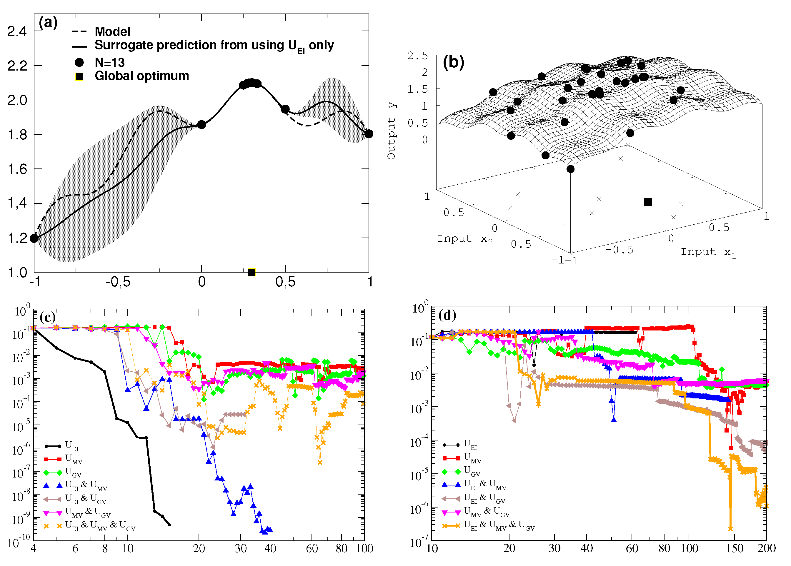
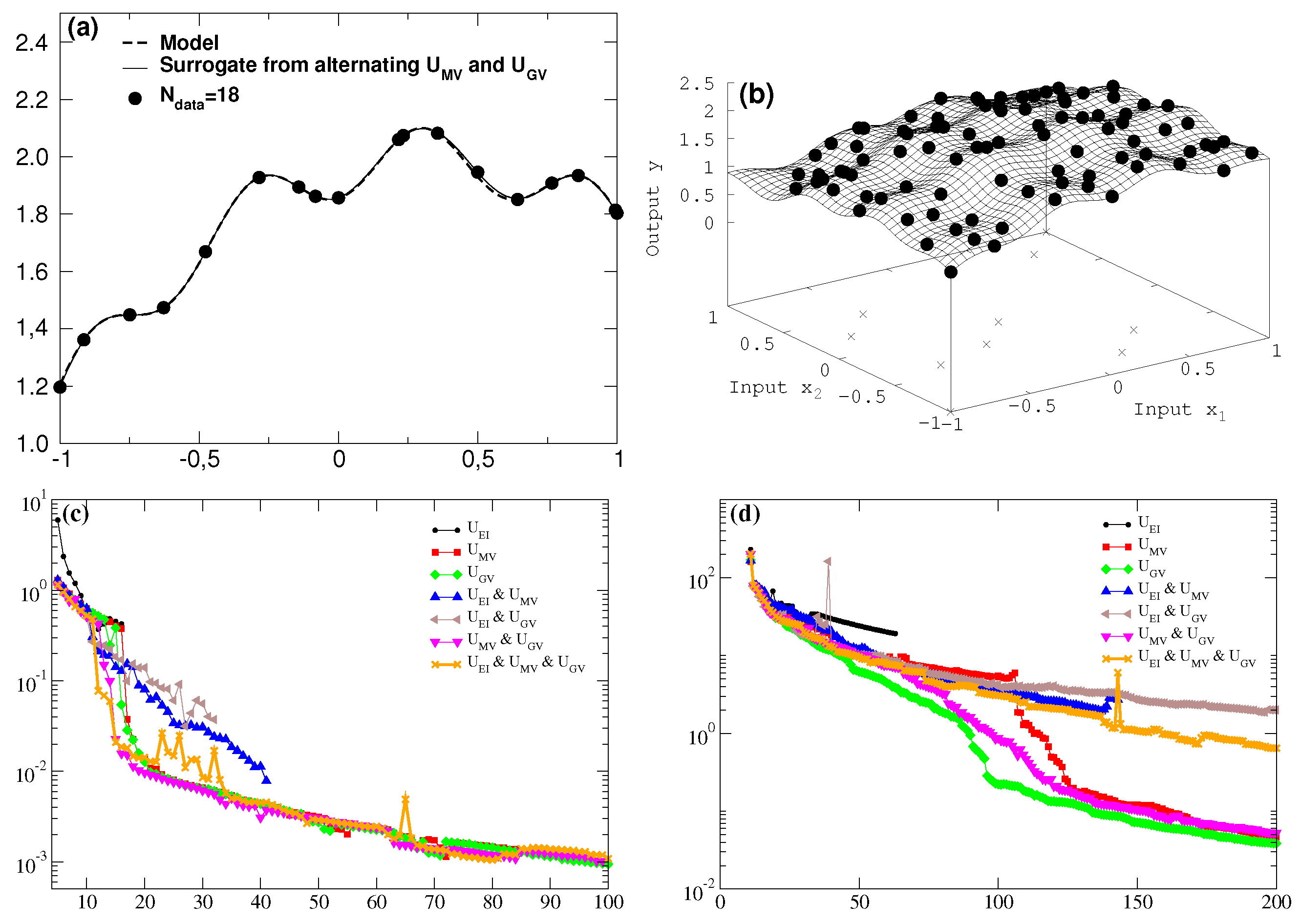
For every newly added data point proposed by the various utilities, the distance between the true location of the global optimum and the maximal value of the surrogate residing on the data at hand is calculated in Figure 1. In a similar fashion, the search for the best surrogate description of the hidden model is shown in Figure 2.

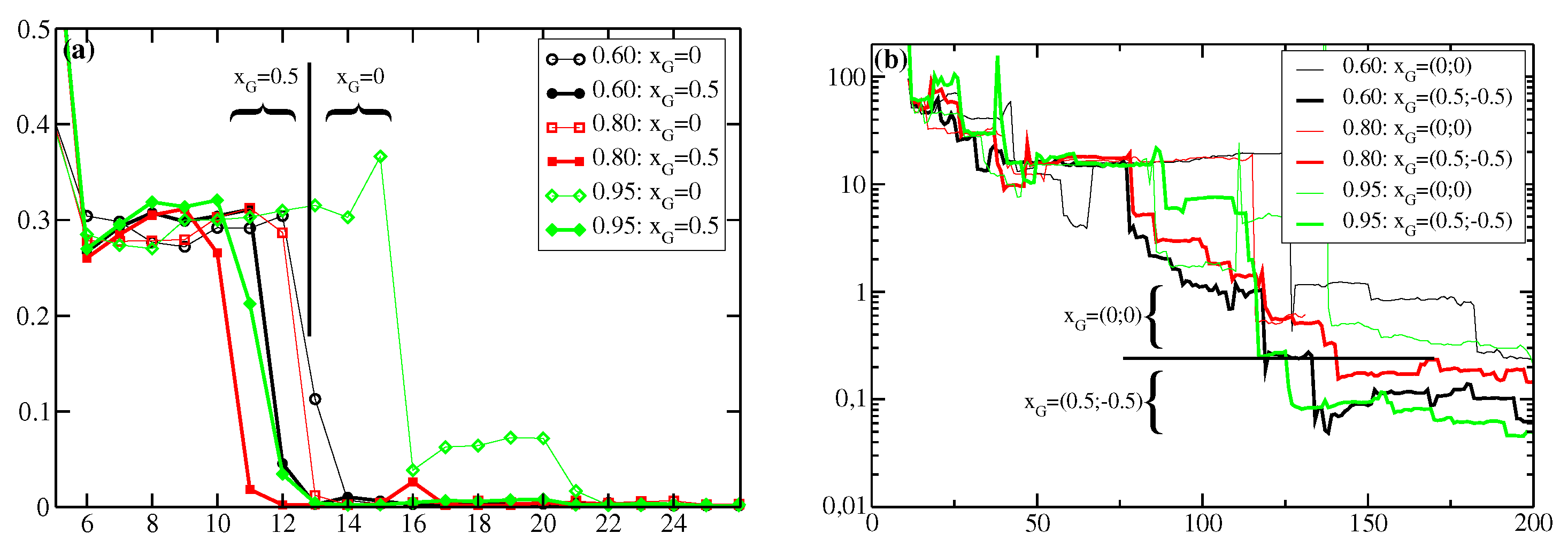
Eventually Figure 3 demonstrates the use of an enveloping Gaussian function in the integral of the global variance by varying its center $x_G$, e.g., if an educated guess about the location of the extremal structure is at hand, i.e., the guiding center $x_G$ is preset to the positive axis (1d) or the quadrant (2d) with the true model maximum. Consequently,

Table 1. Comparison of enveloping Gaussian utilities with different integral weights and guiding centers in finding the best surrogate. 1d: Changing step to solution. 2d: Saturation level of the solution.

Integral Weight of env. Gaussian within RoI	0.6	0.8	0.95
1d: Corresponding width of env. Gaussian ${\sigma }_G$	1.38	0.95	0.71
$U_{\mathrm{GV}}$ with $x_G=0$	15	14	22
$U_{\mathrm{GV}}$ with $x_G=0.5$	13	12	13
2d: Corresponding width of env. Gaussian ${\sigma }_G$	0.99	0.79	0.67
$U_{\mathrm{GV}}$ with ${\mathit{x}}_G$=(0;0)	0.23	0.61	0.21
$U_{\mathrm{GV}}$ with ${\mathit{x}}_G$=(0.5;-0.5)	0.06	0.14	0.05

displays for 1d the specific number of data and for 2d the saturation level for which the target surrogate enters the stage of resembling the true model, i.e. the summed up (absolute) differences between all grid points of the target surrogate and the model starts to diminish with the number of target data only.

4. Discussion

The results above show the usage of various utilities as a toolbox for surrogate modeling. Depending on the task—either to find an extremum or to get a best surrogate description of an unknown “black box” model—and depending on the prior knowledge at hand—presumption of location of the sought extremum or concentration on the region of interest—it is advisable to choose the most eligible utility function. However, even more promising is the combination of utilities of different character to profit from their benefits in toto and to compensate for pitfalls and drawbacks of one or the other utility.

As can be seen in the very first example in Figure 1 for the one-dimensional case the global optimum is found very fast with help of the expected improvement utility $U_{EI}$ (starting to enter the bump with the correct extremum already below N = 10). However, a known drawback of this utility is that it gets stuck in local extrema and that it takes an unreasonably high number of additional data to get distracted from this pitfall.

This is taken into account for the two-dimensional case where the best result with lowest difference to the exact result is obtained by acting in combination of all three utilities $U_{\mathrm{EI}}$, $U_{\mathrm{MV}}$ and $U_{\mathrm{GV}}$. Focusing the maximum search on the utility regarding expected improvement alone (black line in Figure 1d would have got stuck in a local extremum with y = 2.03 in the “wrong” quadrant at (−0.26; −0.29) for not recovering from this at all at about N = 63 (internal stop of algorithm for no improvement after entering computing accuracy level) and totally missing the true optimum with y = 2.2 at (0.3; −0.3).

The situation changes for the task of getting a best overall description within the region of interest. To accomplish this the newly introduced global variance utility $U_{\mathrm{GV}}$ is of tremendous help both in one and two dimensions—either alone or in combination with at least the maximum variance utility $U_{\mathrm{MV}}$. As shown in Figure 2d the best surrogate can already be established around ninety data points by employing $U_{\mathrm{GV}}$ only (full circles in the target surface of Figure 2b, with very few deviations from the true model left.

A guess about the approximate occurrence of an extremal structure–without excluding another region—can be emphasized by a further refinement to the global variance utility. In letting act an enveloping Gaussian within the global variance integral Equation (5) the result is not only much easier to be tackled from a computational point of view, but also the focus of the numerical search for the global optimum can be guided by predetermining the center of Gaussian $x_G$ and its integral weight (aka width ${\sigma }_{x_G}$).

Figure 3 shows the results for three different integral weights (0.6; 0.8; 0.9) of the enveloping Gaussian function at two guiding centers: the first one at the origin corresponds to an ignorant scenario where one is not sure about a certain position of some global optimum at all. In the second approach we suppose that the extremal structure may be found in one dimension for positive values and thereby set $x_G=0.5$, while in two dimensions it may be located within the quadrant with positive values for $x_1$ and negative ones for $x_2$ resulting in $x_G=[0.5;-0.5]$. As can be seen already in Figure 3, but all the more learned from the numbers of Table 1, displacing the center of the enveloping Gaussian function to the real center of the optimum of the hidden model facilitates the development of a best—regarding similarity to the true model—surrogate surface.