Abstract
Accurate day-ahead solar forecasting is essential for grid stability and energy planning. This study introduces a specialized forecasting framework that enhances accuracy by training models on specific day-to-day sky condition transitions. The framework employs a dual-attention transformer model, which captures complex temporal and feature-wise relationships, using a dataset of approximately 5000 daily sequences from three sites in Mongolia (2018–2024). Our core contribution is a specialized training strategy where the dataset is first classified into nine distinct classes based on the sky condition transition from the previous day to the forecast day, such as ‘Clear’ to ‘Partly cloudy’. A dedicated transformer model is then trained for each transitional state, enabling it to become an expert on that specific weather dynamic. This specialized framework is benchmarked against a naive persistence model, a standard, generalized transformer trained on all data and a ‘cluster-then-forecast’ approach. Results show the proposed approach achieves superior performance improvement compared to baseline models (p < 0.001) across all error metrics, demonstrating the value of modeling inter-day weather dynamics. Furthermore, the framework is extended to probabilistic forecasting using quantile regression to generate 80% prediction intervals, providing crucial uncertainty information for operational decision-making in power grids.
1. Introduction
Solar forecasting plays a crucial role in the effective planning and management of power grids by predicting the most likely future solar resource scenarios. Compared to other energy forecasting domains, such as load, price, and wind forecasting, solar forecasting remains relatively immature. This disparity stems from the greater variability of solar irradiance and the relatively lower market integration of solar power systems [1,2].
Similar to wind forecasting, solar forecasting is broadly categorized into two approaches: (1) forecasting the solar resource itself, such as solar irradiance, and (2) forecasting the resulting power output from photovoltaic (PV) systems. Since the resource directly influences the generation, forecasts of solar irradiance can be translated into power predictions using PV performance models, often referred to as white-box or parametric models [3]. Accordingly, this study focuses on solar irradiance forecasting, especially the global horizontal irradiance (GHI).
Regarding the forecast horizon, while short-range forecasts on the scale of minutes are for real-time dispatching, long-term forecasts assume several months in the future, which helps maintenance scheduling. Of particular importance is day-ahead forecasting, which supports the optimal scheduling of various generation resources under economic constraints. For this time horizon, numerical weather prediction (NWP) data is frequently utilized due to its capacity to describe atmospheric processes via physical parameterizations. Yet the reliability of NWP forecasts is highly dependent on accurate model initialization, and historical operational forecasts are not always publicly accessible.
Further classifications include deterministic vs. probabilistic and local vs. regional forecasts [3,4]. In the context of probabilistic forecasting, ensemble-based methods are commonly employed. These include combining outputs from multiple NWP members initialized with perturbed conditions [5], or using historical data from past days with similar forecasted weather conditions as an ensemble of possible outcomes [6]. Additionally, Monte Carlo simulations are often used to account for uncertainties in future scenarios. For example, Badosa et al. [7], converted deterministic NWP outputs into probabilistic forecasts by applying a time-dependent stochastic differential equation, which simulates independent trajectories of the clear sky index using calibrated parameters for a given day.
The current status quo of forecasting is harnessing the advancements in artificial intelligence (AI), including machine learning algorithms and neural networks [4,8]. In addition, they can be used in the post-processing routine, such as a bias correction, to improve the forecast accuracy [9,10]. For instance, Verbois et al. [11] proposed a probabilistic post-processing technique for the Weather Research and Forecasting (WRF) model using principal component analysis (PCA) and quantile gradient boosting.
Several recent studies have investigated various deep learning approaches to improve deterministic day-ahead solar forecasting, with long short-term memory (LSTM) networks being among the most widely adopted models. For example, LSTM has been used in microgrid applications to forecast solar power output [12]. Qing et al. [13] applied a single-layer LSTM model to predict hourly GHI for day-ahead intervals between 8 a.m. and 6 p.m., using features derived from weather forecasts. Their model outperformed baseline approaches such as persistence, linear regression, and multilayer perceptron (MLP). In addition to standalone LSTM models, various hybrid architectures have also been explored. For instance, Gramian angular fields are employed to convert past GHI time series into images, which are then processed by convolutional neural networks (CNN) for feature extraction, followed by an LSTM for temporal forecasting [14]. Moreover, several studies have proposed decomposing historical time series into trend and detail components using techniques such as the fast Fourier transform (FFT) and wavelet analysis. These components are then individually modeled to capture temporal dependencies via bidirectional or attention mechanism-based LSTM networks [15,16].
More recently, attention-based [17] transformer architectures have gained significant attention for their potential in various time series forecasting tasks, including spatiotemporal energy meteorology and electricity load forecasting [18,19,20]. These tasks often involve multivariate, multimodal, or multi-channel data, which require efficient modeling of dependencies across different dimensions. To address this, recent studies have proposed methods for cross-dimensional dependency modeling [20,21]. For example, Boussif et al. [22] proposed the Cross Vision Video Transformer (CrossViVit) model, which incorporates multimodal inputs such as direct normal irradiance (DNI), diffuse horizontal irradiance (DHI), pressure, elevation, and satellite imagery collected over 15 years from six geographically diverse European sites. Their 145-million-parameter model achieved superior generalization performance across unseen locations and years. Nevertheless, its utility is often constrained by the high dimensionality and volume of data, which includes numerous spectral channels and vast spatial domains. Other researchers applied similar cross-dimension modeling on multi-channel time series data, but they rely solely on historical data and omit forward-looking features such as forecasted weather variables, which are crucial, especially for day-ahead predictions [23,24].
In a probabilistic forecasting framework, the quantile loss function [22], also known as the pinball loss, has been integrated into neural network architectures to generate prediction intervals. Erdman et al. [24], for example, combined quantile loss with an LSTM network to perform day-ahead hourly probabilistic forecasting of solar irradiance in the Arctic Circle. Although their model outperformed smart persistence and MLP baselines, the prediction intervals occasionally yielded physically unrealistic values (such as below 0 W/m2). Similarly, Huan et al. [25] applied quantile regression to the probabilistic forecasting of regional PV power output, incorporating unsupervised clustering of regional weather patterns to improve accuracy.
To improve performance under varied weather conditions, a more sophisticated ‘cluster-then-forecast’ strategy has been developed. This involves classifying the forecast day into distinct weather types (such as clear, cloudy, or overcast) and training a specialized model for each type [6,26]. However, these advanced methods treat each day in isolation. The classification is based solely on the static characteristics of the forecast day. This overlooks the valuable information contained in the dynamic transition of weather systems, such as the difference between a stable, clear day following another clear day and a clear sky following an overcast day, where the change is more abrupt.
This study addresses this gap by proposing a novel framework that classifies days not by their static state, but by their transitional state based on the sky conditions of both the previous and forecast days. Since it is common practice to classify days into clear, cloudy, and overcast, this study considered nine possible transitions by combining these three sky classes. By training highly specialized models for each transition, our approach aims to better capture the persistence and dynamics of weather patterns, leading to more accurate forecasts, especially during periods of change. The overall view of the current day-ahead solar irradiance prediction techniques, including their main advantages, disadvantages, and error range, is summarized in Table 1.

Table 1.
Summary of the current solar irradiance forecasting methods in the day-ahead horizon. Models are abbreviated as: numerical weather prediction (NWP), Weather Research and Forecasting (WRF), Global Forecast System (GFS), European Centre for Medium-Range Weather Forecasts (ECMWF), Japan Meteorological Agency Global Spectral Model (JMA GSM), moving average (MA), autoregressive moving average (ARMA), seasonal autoregressive integrated moving average (SARIMA), artificial intelligence (AI), artificial neural network (ANN), support vector machine (SVM).
The key contributions of this work are as follows:
- Specialized training by weather transition: A novel forecasting framework is proposed that trains dedicated deep learning models for each of nine day-to-day sky condition transitions, allowing the models to become experts on specific weather dynamics.
- Synergistic feature integration: The effective use of a feature set that combines historical ground-based data with forward-looking cloud cover forecasts to improve predictive accuracy.
- Dual-attention transformer (DAT) for solar forecasting: An encoder-only, dual-attention transformer that efficiently models both temporal and cross-feature dependencies in the multimodal data.
- Systematic performance evaluation: A rigorous benchmarking of the specialized framework against baselines across a wide range of weather scenarios.
- Probabilistic forecast generation: The adaptation of the deterministic model to provide calibrated probabilistic forecasts using quantile regression, enabling the quantification of forecast uncertainty through prediction intervals.
This comprehensive evaluation advances the field of solar forecasting by offering a robust, accessible, and adaptable methodology suitable for deployment across different geographical regions and related downstream tasks, such as forecasting PV output power or the outlet temperature of solar thermal collectors, thereby contributing to improved grid reliability and energy balance.
2. Dataset
2.1. Time Series
This study uses hourly meteorological time series data collected from three major Mongolian cities, namely Ulaanbaatar (47.92° N, 106.92° E), Darkhan (49.46° N, 105.98° E), and Erdenet (49.00° N, 104.01° E). The details of the ground measurement sites are described in [27]. Each site is equipped with sensors to measure wind speed and direction, ambient temperature, relative humidity, and GHI. The specifications of measuring devices are listed in Table 2. In addition, the vapor pressure and dew point temperature are retrieved from the ambient temperature and relative humidity through the Magnus formula. Data collection began in the summer of 2018 and has been ongoing consecutively.
Table 2.
Specifications of the ground site instruments.
To ensure the completeness and reliability of the input sequences, any day containing missing data is entirely excluded. This filtering results in 2050, 1340, and 1553 complete daily records for Ulaanbaatar, Darkhan, and Erdenet, after discarding 12, 6, and 4 incomplete days of measurements, respectively. Figure 1 illustrates the hourly average GHI values recorded at these locations. While continuous measurements are ideal for capturing daily, seasonal, and interannual solar patterns, the dataset includes extended periods of missing data, sometimes exceeding one year, primarily due to power outages or equipment maintenance issues. Nevertheless, since each site contains at least three years of measurements with a fairly balanced seasonal coverage (a slight bias toward summer months), no interpolation or data imputation methods are applied; the original observations are retained as they are.
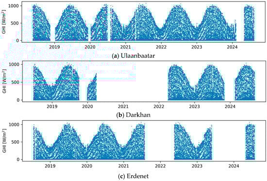
Figure 1.
Hourly average global horizontal irradiance (GHI) records at ground sites.
In addition to the raw meteorological features, several derived features are computed: hour of the day (HH), day number (DN), solar zenith angle (ZA), solar azimuth angle (AA), and clear sky global horizontal irradiance (CS GHI). These calculations use the default Ineichen model with climatological turbidity as implemented in the Python pvlib 0.10.4 library [28]. Moreover, since cloud information is one of the most influential factors affecting surface irradiance, hourly cloud cover data was retrieved from the ERA5 reanalysis dataset with a spatial resolution of 0.25° (approximately 27.6 km at the equator) [29]. It is important to note that, because ERA5 is a reanalysis product (describing past weather based on ground observations), actual day-ahead cloud cover forecasts should be used when deploying in real-world applications, such as operational cloud forecasts from the Global Forecast System (GFS) [30] and European Centre for Medium-Range Weather Forecasts (ECMWF) [31]. It is assumed that the proposed GHI forecasting framework would be able to tolerate input uncertainties for this transition, as ERA5 data carries inherent uncertainties due to its lower spatial resolution and limited number of assimilated ground observations.
To further contextualize the data, daily sky conditions are analyzed using the clear sky index (CSI), defined as the ratio of the observed GHI to the corresponding clear sky irradiance. Based on the daily mean CSI (), each day is classified into one of three categories as shown in Equation (1).
Figure 2 shows the results of this classification. Clear sky conditions dominate across all three sites, accounting for 55.9–59.7% of the total records. Partly cloudy and overcast days represent 33.9–35.5% and 6.2–8.6% of the data, respectively. While this classification is not used as a direct input feature in the forecasting model, it offers valuable context for evaluating model performance under different sky conditions.
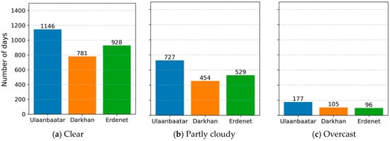
Figure 2.
Daily sky condition classification.
To better understand the strengths and limitations of various solar forecasting models, forecasting scenarios are defined by combining the sky conditions of the forecast day with those of the previous day. This yields nine possible two-day sky condition scenarios, as shown in Figure 3. The most frequent case is a clear day followed by another clear day, accounting for approximately 38.75%. In contrast, combinations involving overcast days are much less common—ranging from 3.60% to 1.75%—reflecting the predominance of clear skies in the dataset. The remaining transitions between clear and partly cloudy conditions collectively represent around 45.3% of the total cases.
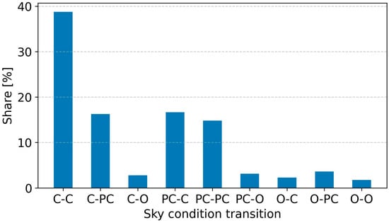
Figure 3.
Distribution of sky condition transitions across all data. Day classes are abbreviated as: clear (C), partly cloudy (PC), and O (overcast). The dash represents the transition from the previous day to the forecast day.
2.2. Pre- and Postprocessing
To prepare the data for modeling, daily records were reformatted into continuous two-day sequences, where the first day represents the previous day and the second day serves as the forecast day. It is important to note that, in a continuous time series of d daily records, every day except the first and last can serve as both a forecast day and a previous day. This approach yields d − 1 usable data blocks. Due to interruptions in data collection —specifically 11 in Ulaanbaatar, 3 in Darkhan, and 5 in Erdenet—the final number of valid samples was 2038, 1336, and 1547, respectively. Rather than using full 24 h data, only the period from 9:00 a.m. to 6:00 p.m. was considered for each day. This time window was selected because early morning and late evening irradiance levels are typically low, even during longer summer days, making their exclusion negligible in terms of energy contribution.
In a supervised learning context, models require both input features and corresponding output labels to learn meaningful relationships. Here, the input features are the meteorological variables from the previous day and solar position, clear sky irradiance, and cloud cover for the forecast day. Figure 4 presents scatter plots between each input feature and the output target, which is the day-ahead GHI. Visual analysis reveals moderate positive correlations between the target and variables such as ambient temperature, dew point temperature, and clear sky GHI. The solar zenith angle shows a clear negative correlation, which is expected as higher zenith angles correspond to lower solar elevations. Features such as the hour of the day, azimuth angle, and day number reflect the diurnal and seasonal patterns of solar movement and intensity.
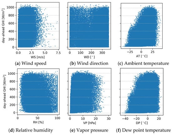
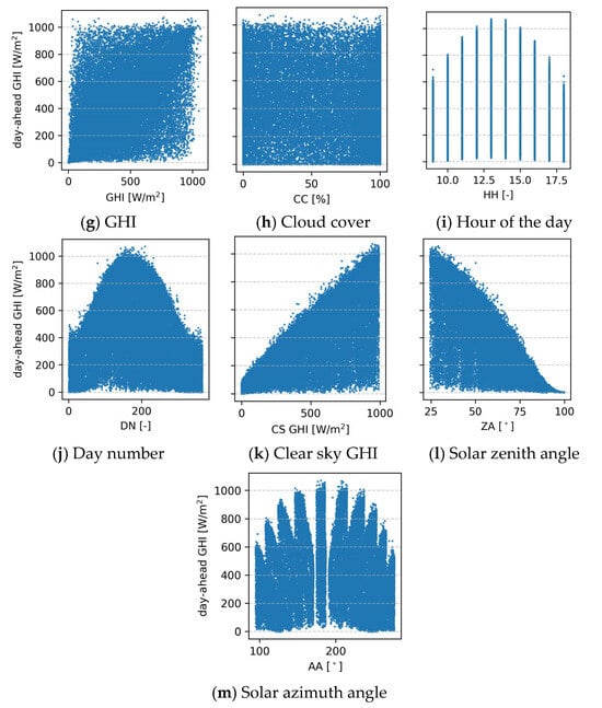
Figure 4.
A scatter plot between the input features in the horizontal axis and the output target in the vertical axis.
Table 3 quantifies these relationships using correlation coefficients, highlighting that the most influential predictors of next-day GHI are the previous day’s GHI and the corresponding clear sky GHI and zenith angle in the day-ahead horizon. This is intuitive, as the clear sky GHI represents the theoretical maximum irradiance under ideal conditions, the zenith angle determines the sun’s position, and the previous day’s GHI reflects prevailing atmospheric conditions that can influence the following day’s solar potential.
Table 3.
The correlation coefficients between the input features and the output target (day-ahead GHI). Input features are abbreviated as: wind speed (WS); wind direction (WD); ambient temperature (AT); relative humidity (RH); vapor pressure (VP); dew point temperature (DP); cloud cover (CC); hour of the day (HH); day number (DN); clear sky global horizontal irradiance (CS GHI); solar zenith angle (ZA) and azimuth angle (AA).
For feature selection, a correlation coefficient threshold of 0.1 was applied to identify the most relevant predictors. Based on this criterion, all meteorological parameters except wind direction were retained in addition to the previously identified highly correlated features. Interestingly, cloud cover showed a weak, negative correlation with surface irradiance. This is likely due to the complex, non-linear relationship between cloud characteristics and surface irradiance; for example, thin or semi-transparent clouds may only slightly reduce irradiance, whereas thick clouds can significantly block it. Despite the weak linear correlation, cloud cover was retained as an input feature due to its clear but non-linear inverse relationship with GHI. Features that were found to be redundant or less informative were excluded. Specifically, azimuth angle, hour of the day, and day number were removed since their effects are already encapsulated within the clear sky irradiance. As a result, the number of input features was reduced from 13 to 9, improving model efficiency and reducing computational overhead without compromising predictive capability.
In the final preprocessing step, both input and output values are normalized using min-max scaling. This improves the convergence of the training process by standardizing feature ranges and enabling more stable weight updates. The processed two-day blocks, containing both explanatory and response variables, are then classified into respective sky condition transitions, as illustrated in Figure 3, and randomly shuffled within this category to ensure generalization across different locations and seasonal conditions. This specialized training framework is designed to improve forecasting accuracy by allowing the model to become an expert on specific weather dynamics. For instance, a model trained exclusively on ‘Clear-to-Overcast’ transitions can focus on learning the distinct meteorological patterns associated with an approaching weather front, without its learning process being dominated by the more frequent and less complex ‘Clear-to-Clear’ transitions. We hypothesize that this approach, by isolating and dedicating resources to less common but challenging weather events, will yield a more accurate and robust forecasting system compared to a generalized model trained on the entire, unclassified dataset.
In the post-processing stage, any negative predictions are corrected by setting them to 0 W/m2.
3. Methodology
3.1. Persistent Model
The persistence model assumes that the hourly GHI values from the previous day will persist unchanged into the forecast day. This can be mathematically expressed by Equation (2).
where is the predicted GHI for hour on day , and is the measured GHI for the same hour on the previous day. Despite its simplicity, the persistence model often performs well in short-term forecasting and under stable atmospheric conditions, such as transitioning from clear day to clear day, making it a commonly used baseline for evaluating the performance of more advanced forecasting models.
3.2. Dual-Attention Transformer
At the core of the transformer architecture is the attention mechanism, specifically scaled dot-product attention [17]. This mechanism enables the model to focus on different parts of the input sequence when encoding a particular element, allowing for a more flexible and context-aware representation of sequential data.
In time series forecasting, the raw input sequence is first represented as a matrix , where is the number of time steps (10 in this case), and is the number of input features per time step (9 in this case). Each time step is then projected into a higher-dimensional space () using a learnable linear embedding as formulated in Equation (3). This embedding can be combined with positional encodings (fixed or learnable), which help the model retain information about the temporal order, an essential factor in time series modeling.
Each embedded vector (each time step) is linearly projected into three vectors:
- Query ()—determines what the model is looking for,
- Key ()—contains information that may be relevant to a query,
- Value ()—the actual content to be aggregated or passed through.
These are obtained by multiplying the embedded input vector by learned weight matrices as in Equation (4).
where and are the dimensions of the key/query and value vectors, and usually they are the same.
Then, attention scores are calculated using the dot product between the query and all keys by Equation (5). This computes a weighted sum of the values, where weights are determined by the compatibility of the query with the corresponding keys. This allows the model to aggregate context from all time steps in a sequence, dynamically attending to the most relevant ones.
To enable the model to capture different types of temporal dependencies and relational patterns simultaneously, multi-head attention is applied. This involves running the attention mechanism in parallel across multiple subspaces, known as heads, as expressed by Equation (6). The number of attention heads is usually . Each head learns a distinct representation of the input by attending to different aspects or time steps. The outputs from all heads are concatenated and transformed through a final linear projection.
The transformer encoder consists of multiple stacked layers, each composed of:
- Multi-head self-attention (to capture contextual relationships), and
- Position-wise feed forward network (to model feature interactions independently at each time step)
Each of these components is followed by a residual connection and layer normalization; thus, the encoder layer can be expressed by Equation (7).
where feed forward dimension is usually set to , and the Gaussian Error Linear Unit (GELU) activation function is employed to introduce non-linearity. These stacked encoder layers process the entire input sequence in parallel, unlike recurrent neural network (RNN) based models that process sequentially.
A transformer decoder is not necessary in this study because the task is to generate a continuous sequence of predictions in parallel without requiring autoregressive decoding. Correspondingly, the encoder effectively serves as both a feature extractor and a forecasting mechanism. The encoder-only design also reduces model complexity and training time, while still benefiting from the attention mechanism’s ability to model long-range dependencies within the input sequence. This makes it especially well-suited for day-ahead forecasting tasks where all input data is available upfront.
To capture both temporal dynamics and inter-feature dependencies in the inputs, the DAT is proposed, as illustrated in Figure 5. Unlike the standard temporal transformer, which applies attention only across time while treating each feature independently, our model introduces a two-stage hierarchical attention mechanism: feature-wise and temporal attention. In the first stage, feature attention is applied independently at each time step, enabling the model to dynamically learn context-dependent relationships among meteorological and solar variables such as ambient temperature, relative humidity, and solar irradiance. This is achieved by embedding all features into a shared latent space with learnable feature-wise positional encodings, followed by multi-head self-attention. The output at each time step is aggregated into a single vector that represents the cross-feature context. To mitigate overfitting, dropout layers are inserted within the feature embedding and aggregation layers.
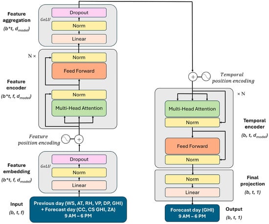
Figure 5.
Dual-attention transformer (DAT) model for day-ahead solar irradiance forecasting. Dimensions are notated as: (batch size), (time steps), (features) and (model size). is the number of stacked layers in the encoder.
In the second stage, this feature-aware temporal sequence is processed by a temporal attention module, where positional encodings are added to maintain the sequence order, and multi-head self-attention captures the inter-hour dependencies throughout the forecast day. The final encoder output has the shape , capturing the enriched representations of the corresponding 10 h in the previous and forecast days. This output is passed through a linear projection layer that maps it directly to the day-ahead GHI forecast.
This dual-attention design is particularly well-suited for solar irradiance forecasting because it allows the model to jointly reason over both instantaneous meteorological conditions and their temporal evolution, especially under varying weather conditions. Compared to standard transformer-based approaches, this architecture explicitly disentangles and then fuses feature- and time-level dependencies, leading to improved generalization and interpretability in complex weather scenarios.
3.3. Probabilistic Forecasting by Quantiles
To extend the day-ahead solar irradiance forecasting framework for a probabilistic setting, quantile regression is employed, allowing for the prediction of intervals rather than single-point estimates. Unlike traditional regression methods that estimate the conditional mean, quantile regression estimates specific conditional quantiles of the response variable. This is achieved by minimizing an asymmetric pinball loss function defined as in Equation (8).
Here, ω ∈ (0,1) represents the quantile level and and are the true and predicted values, respectively.
- When ω = 0.5, the model penalizes over- and under-predictions equally, yielding the median forecast.
- If ω > 0.5, the model penalizes under-predictions more heavily, pushing more observations above the forecast line.
- Conversely, if ω < 0.5, over-predictions are penalized more, resulting in more points below the forecast.
Accordingly, the proposed DAT architecture shown in Figure 5 has been extended to capture the uncertainty associated with day-ahead GHI forecasts by generating probabilistic outputs. Instead of producing a single-point (such as median) prediction, the model is retrained to predict multiple quantiles of the target variable. In this study, a denser set of quantiles is used: [0.1, 0.2, 0.3, 0.4, 0.5, 0.6, 0.7, 0.8, 0.9], which supports the construction of an 80% prediction interval while preserving the structure of the full predictive distribution. Such a detailed representation is especially valuable in solar forecasting, where high variability under partly cloudy conditions can lead to complex, non-Gaussian distributions that cannot be adequately captured by a single interval.
3.4. Implementation
Both the deterministic and probabilistic versions of the DAT were implemented in PyTorch (v2.6.0). The models were trained on an NVIDIA (Santa Clara, CA, USA) RTX A4000 GPU with 16 GB of VRAM. The deterministic model utilized the mean squared error (MSE) to minimize forecasting error, while the probabilistic model was trained with the pinball loss to generate accurate predictive quantiles. This selection of loss functions ensures that each model is appropriately optimized for its respective forecasting task—point prediction versus uncertainty estimation.
In both deployments, a learning rate scheduler illustrated in Figure 6 is employed for efficient convergence. During the first 10% of the total training steps, the learning rate gradually increases (warm-up phase), after which it enters a cosine annealing phase. The minimum learning rate is 0.1% of the maximum value to ensure the learning continues. Accordingly, if the maximum learning rate is 10−4, the minimum learning rate will be 10−7. Furthermore, each model is trained for 100 epochs using the AdamW optimizer, which incorporates L2 regularization via weight decay to penalize large weights and thereby control model complexity.
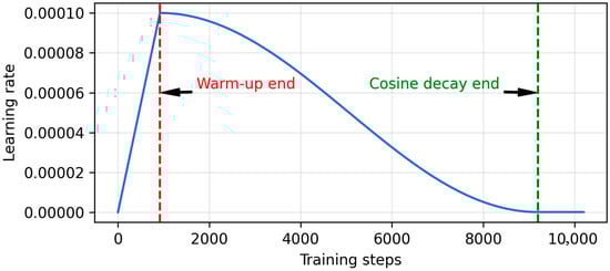
Figure 6.
Linear warm-up + cosine decay learning rate scheduler.
The model architecture and training hyperparameters were optimized through a fine-tuning process on a dedicated data split, comprising 60% and 20% of all data for training and validation. The validation split helps ensure that the model is not overfit to the training data by encouraging it to learn general tendencies rather than memorizing specific data. The optimal configuration was found to be a batch size of 32, a weight decay of 10−3, a maximum learning rate of 3 × 10⁻⁵, and a dropout rate of 0.1. The transformer’s internal model dimension () was set to 256.
With these optimized hyperparameters fixed, the final models were trained for each of the nine sky condition transitions. To ensure robust and unbiased evaluation, a 5-fold cross-validation scheme is employed to train an ensemble of five models on 80% of the data within each class. The final prediction for each class is the arithmetic mean of this 5-model ensemble. The final 20% of data for each class was reserved as a test set for the independent performance assessment.
3.5. Evaluation Metrics
The mean absolute error (MAE) and root mean square error (RMSE) defined in Equations (9) and (10) are used to evaluate the predictive performance of the deterministic forecasting [4]. Since each input-output sample corresponds to a full day (9:00 a.m. to 6:00 p.m.), the error metrics are computed on a daily basis and then averaged over the number of evaluated days ().
For evaluating probabilistic forecasts, the MAE and RMSE of the median forecast are used. Additionally, to further assess the quality of the prediction intervals formed between the 10th and 90th percentiles, interval coverage (IC) is calculated as the proportion of observed values that fall within the predicted range, as written in Equation (11) [24]. An ideal 80% prediction interval should yield an IC close to 80%. In parallel, the average interval width (AIW) evaluates the sharpness of the forecast by averaging the width of the prediction intervals over all time steps, as in Equation (12) [6]. While high coverage ensures reliable predictions, overly wide intervals indicate poor resolution; thus, AIW serves as a counterbalance metric.
4. Results
4.1. Deterministic Forecasting
The forecasting performance of the four models—the baseline persistence, the generalized DAT trained on all data, specialized DAT considering weather types in the target forecast day like ‘cluster-then-forecast’ strategy and the specialized DAT integrating nine transitions—is summarized in Table 4. This section analyzes their performance across all sky conditions and for specific transitional states.
Table 4.
Test error metrics in W/m2 classified by sky condition transitions. Values are presented as mean ± 95% confidence interval margin of error. The mean value represents the error of the final ensemble average, while the margin of error is derived from the performance of the five individual models that constitute the ensemble. The dash represents the transition from the previous day to the forecast day. The best error metrics are underlined.
As expected, the persistence model serves as a lower bound for performance, yielding the highest overall errors with an all-sky MAE of 124.87 W/m2 and RMSE of 195.43 W/m2. Its performance varies significantly with weather stability; it performs best during consecutive clear days (MAE: 47.55 W/m2 and RMSE: 84.50 W/m2) but fails dramatically during highly dynamic transitions, such as from overcast to clear conditions (MAE: 310.72 W/m2 and RMSE: 377.78 W/m2). This highlights the limitations of naive methods during periods of atmospheric change.
The proposed specialized DAT framework, where a dedicated model is trained for each of the nine sky condition transitions, achieves the best overall performance. It records an all-sky MAE of 70.36 W/m2 and RMSE of 106.84 W/m2, representing a substantial error reduction of 54.51 W/m2 (44%) and 88.59 W/m2 (45%), respectively, compared to the persistence baseline. The benefits of specialization are most pronounced during challenging transitions involving clear and overcast skies, where error reductions of over 200 W/m2 are observed. By focusing on a single weather dynamic, the specialized models are better able to capture the abrupt changes in irradiance characteristic of these events. Conversely, for stable conditions like consecutive clear or overcast days, the improvement over the strong persistence baseline is more modest, reducing MAE by 10.29–21.59 W/m2 and RMSE by 24.98–41.30 W/m2.
To quantify the specific benefit of the specialized training strategy, a generalized and 3-class specialized DAT versions were trained on the entire cross-validation dataset. These models also significantly outperform the persistence baseline with all-sky MAE of 75.69–82.03 W/m2 and RMSE of 111.75–125.57 W/m2. For all scenarios except the continuous overcast days, the generalized DAT performed superior to the naïve persistent, demonstrating the power of the underlying DAT architecture. However, these two implementations are consistently inferior to the specialized framework, accounting for 9 transitions, with its all-sky MAE and RMSE being higher by 5.33–11.67 W/m2 and 4.91–18.73 W/m2, respectively. The uncertainty is also higher for these compared to the narrower confidence intervals of the specialized 9-class DAT configuration. Particularly, the generalized model’s performance suffered from having to learn an average representation across all weather dynamics, which diluted its effectiveness for any single transition type.
To verify the statistical significance of the observed improvements, a Wilcoxon signed-rank test was performed. The test compared the daily RMSE scores of the proposed specialized DAT model with 9-class against the baselines. The results show that the specialized 9-class DAT model performs significantly better than the other 3 models (p < 0.001). This provides strong evidence that the performance gains from our transition-based framework are consistent and not a result of random chance.
Moreover, the performance of the forecasting models is visualized by a residual plot in Figure 7. An analysis of the residual plots reveals distinct error patterns among the models. As described earlier, the naïve persistent model exhibits highly erratic behavior, with frequent extreme under- and overpredictions (residuals reaching up to 900 W/m2). In contrast, DAT implementations, particularly the specialized version with 9-class sky transitions, produce forecasts that align more closely with the ground truth values, indicating improved accuracy. Although the scatter plot of the specialized DAT implementations looks similar, there is a significant clustering for the 3-class, while the plot is smoother for the 9-class transitions.
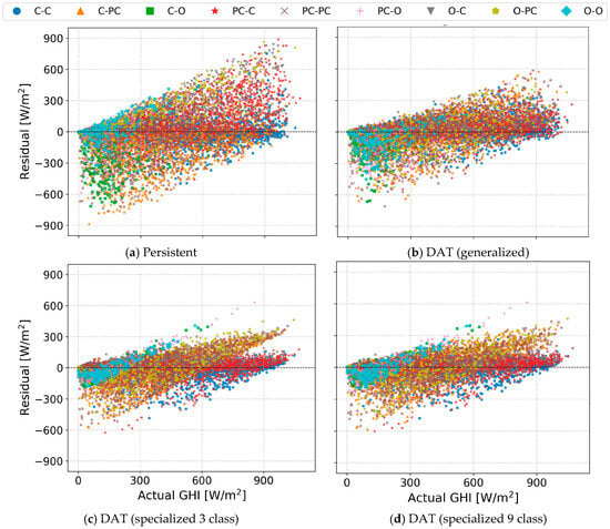
Figure 7.
Residual (true-predicted) plot of the predicted day-ahead hourly GHI by various models. Different weather dynamics are illustrated by different colors.
For stable scenarios like consecutive overcast days, both the persistence model and the generalized DAT exhibit significant bias, tending to either under- or over-predict GHI. In contrast, the specialized DAT models for this condition show a more centered residual distribution, effectively minimizing this systematic bias. A similar pattern is observed for consecutive clear days, where the specialized models’ residuals are clustered near zero, indicating higher accuracy with a slight tendency for over-prediction.
The most substantial improvements from the specialized framework are observed during dynamic transitional scenarios, particularly for ‘Partly cloudy-to-Clear’, ‘Clear-to-Partly cloudy’, and ‘Clear-to-Overcast’ transitions. This confirms that dedicating a model to these specific dynamics allows for a more accurate capture of their unique irradiance profiles.
Despite its superior performance, the specialized DATs exhibit some remaining error signatures. It occasionally over-predicts GHI by up to 600 W/m2 during low-irradiance periods (early morning and late afternoon) and can under-predict during peak irradiance hours. These limitations are likely attributable to uncertainties in the input cloud cover. Future work should therefore focus on incorporating more granular atmospheric variables or advanced cloud forecasts to further refine model performance during these challenging periods.
To further visualize the forecasting in action, Figure 8 illustrates the forecasting results for representative days selected from each of the nine transitional states. For stable, consecutive, clear-sky conditions, all models, including the baseline, perform well as expected. The advantages of the deep learning frameworks become apparent during dynamic transitions. When a clear day is followed by a partly cloudy or overcast day, all DAT models correctly predict a significant reduction in GHI, adapting far better than the naive persistence forecast. Conversely, when predicting a clear day that follows a cloudy or overcast day, the DAT predictions are nearly identical and accurately capture the sharp recovery of irradiance to clear-sky levels.
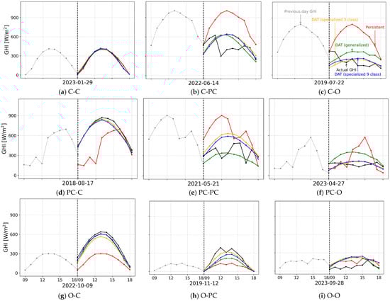
Figure 8.
Forecasting under different sky condition transitions. The vertical axis shows the GHI in W/m2, while the x-axis title shows the forecast date. The vertical dashed line shows the forecast start.
The most distinct advantage of the specialized framework is observed in the highly stochastic transitions between partly cloudy and overcast conditions. In these scenarios, the specialized DATs’ predictions align most closely with the actual GHI values. While these models capture the correct daily magnitude of irradiance, they generate a smoothed, bell-shaped curve rather than replicating the high-frequency fluctuations characteristic of partly cloudy skies. Finally, for stable overcast conditions, all models follow the general trend of the ground truth GHI, though they all exhibit a slight tendency to over-predict.
The improved accuracy of the specialized framework, considering 9 sky transitions, introduces a trade-off in deployment complexity. While the DAT architecture for any single model instance contains 6.4 million parameters, the full specialized system requires storing nine distinct 5-model ensembles, resulting in a significantly larger storage footprint than the single ensemble of the generalized model. Nonetheless, this is a static cost. Crucially, there is no significant difference in training time, as the total number of samples processed remains constant. Furthermore, the inference speed is nearly identical, as generating a forecast only requires a simple classification step to select and load the appropriate specialized model for the given sky condition.
4.2. Probabilistic Forecasting
In the probabilistic forecasting settings, the DAT model is also aware of the specific weather transition when predicting intervals, similar to that of specialized DAT in a deterministic forecasting context. The analysis of the probabilistic forecasts reveals a direct relationship between forecast uncertainty and sky condition. Figure 9 shows the probabilistic forecasting results on selected days from the test split. Overall, the 80% prediction intervals defined between the 10th and 90th percentiles successfully encompass the true GHI values in most scenarios.
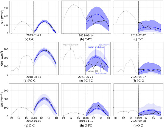
Figure 9.
Probabilistic forecasting performance under different sky condition transitions. The vertical dashed line shows the forecast start. The dash represents the transition from the previous day to the forecast day. The x-axis title shows the forecast date. The same days presented in Figure 8 are also illustrated here. Note: Since the optimal prediction interval is selected from within the range between the 10th and 90th quantiles, the best prediction interval overlaps with the fixed 80% prediction interval. As a result, while the best prediction interval is visualized correctly, the 80% interval may appear narrower than it actually is. To interpret the visualization accurately, the lighter area should be considered as the additional range that, when combined with the best interval, constitutes the full 80% prediction interval.
As expected, the prediction intervals are sharpest for stable, clear-sky days, reflecting the low inherent variability of irradiance under these conditions. Depending on the previous day’s condition, the prediction interval can become slightly wider compared to consecutive clear days. Conversely, for partly cloudy days, the framework generates significantly wider intervals. This demonstrates that the model has successfully learned to associate the high stochasticity of GHI caused by intermittent cloud cover with greater predictive uncertainty. For overcast days, the prediction interval width is typically moderate, reflecting a lower but still present level of variability compared to a clear sky.
In terms of error metrics, the MAE and RMSE of the median prediction (50th quantile), along with interval coverage and average interval width for the probabilistic forecasting defined between the 10th and 90th quantiles, are reported in Table 5. Compared to the deterministic model (Table 4), the test error metrics of the median prediction are slightly different due to the distinct loss functions used during training. The deterministic model was optimized using MSE, which targets the conditional mean, while the probabilistic model’s median is optimized via the pinball loss, which targets the conditional median. Since the mean and median of a distribution are not always identical, especially in skewed distributions common to solar irradiance, there are slight variations in the final error metrics, even though both forecasts aim to capture the central tendency of the data.
Table 5.
Test error metrics of the probabilistic forecasting by the specialized DAT with 9 classes. Values are presented as mean ± 95% confidence interval margin of error. The mean value represents the error of the final ensemble average, while the margin of error is derived from the performance of the five individual models that constitute the ensemble. The dash represents the transition from the previous day to the forecast day.
However, since the main goal of probabilistic forecasting is not centered on median accuracy but on the reliability of the predicted intervals, interval coverage and prediction interval width are used to quantify the model performance. The overall IC was 90.71%, which is higher than the expected 80% coverage for the interval defined between the 10th and 90th quantiles. This suggests that the model’s prediction intervals are slightly over-conservative. The AIW width was 273.22 W/m2, representing the typical spread between the upper and lower bounds.
The width of the prediction intervals varies logically with the predictability of the transitional weather state. The sharpest intervals are generated for transitions culminating in a clear sky, such as ‘Clear-to-Clear’ and ‘Partly cloudy-to-Clear’, with average widths ranging from 153.80 to 237.31 W/m2. This reflects the low uncertainty associated with clear-sky conditions, where the GHI profile is highly deterministic.
Conversely, the model assigns the highest uncertainty to transitions involving a partly cloudy or overcast day, with average widths spanning from 324.00 to 499.28 W/m2. This demonstrates that the probabilistic framework has successfully learned to quantify the significant inherent stochasticity caused by intermittent cloud cover, which makes precise GHI prediction exceptionally challenging.
Since prediction intervals formed between the 10th and 90th quantiles were occasionally unnecessarily wide—such as on 9 October 2022 and 21 May 2021—the optimal prediction interval for each day is determined and denoted as the best interval in Figure 9. The optimal interval selection criteria are:
- If the actual GHI variation is fully contained within the 80% prediction interval, the narrowest possible interval that still captures all the GHI values is selected by adjusting the upper and lower quantiles accordingly.
- If the GHI occasionally exceeds the 90th quantile but remains above the 10th, the upper bound is fixed at the 90th quantile, while the lower bound is selected as the quantile that closely contains the lower range of GHI variation.
- Similarly, if the GHI occasionally drops below the 10th quantile but stays below the 90th, the lower bound is fixed at the 10th quantile, and the upper bound is selected based on the upper range of the observed GHI.
- If the GHI values fall outside both the 10th and 90th quantiles, the full 80% interval is retained without modification.
As a result of applying this adaptive interval selection, it was found that on 543 out of 988 test days, the actual GHI values fell entirely within the 80% prediction interval. While the IC remained unchanged at 90.71%, all-sky AIW was significantly reduced to 209.21 W/m2, marking a decrease of 64.01 W/m2 compared to the fixed 10–90% interval. It should be noted that the optimal interval was selected after observing the ground truth values, and thus does not represent a true probabilistic forecast. Rather, it serves to evaluate the appropriateness of using a fixed 80% prediction interval.
The distribution of the selected optimal quantiles is illustrated in Figure 10. As highlighted in yellow and green shades, the optimal prediction intervals frequently align closely with the 10th and 90th quantiles—particularly during transitions between clear and partly cloudy conditions. This observation supports the appropriateness of using the 80% prediction interval for probabilistic forecasting.
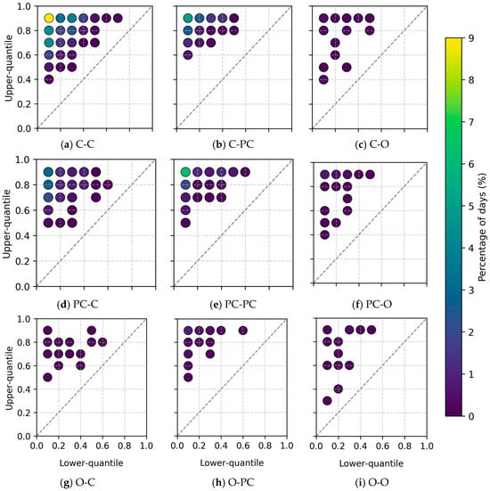
Figure 10.
Distribution of optimal upper and lower quantiles selected to enclose the actual GHI values for each test day.
In detail, on days forecasted to be clear, the upper quantile was typically above 0.4. Conversely, on overcast days, the lower quantile falls below 0.5, due to the expected suppression of irradiance. Although adaptive quantile selection allowed for the dynamic determination of the upper and lower bounds, the optimal prediction intervals that differed from the standard 0.1–0.9 range were relatively rare. Nevertheless, by tailoring the upper and lower bounds to the predicted weather condition, it is possible to narrow the prediction interval, thereby improving forecast sharpness and potentially reducing over-allocation of system resources. Therefore, future research should be directed towards narrowing the interval width while keeping the intended interval coverage.
5. Conclusions
This study introduced a novel day-ahead solar forecasting framework that significantly improves accuracy by training models on specific day-to-day sky condition transitions. By training a specialized DAT for each of nine distinct weather dynamics, the models become experts at predicting the unique irradiance profiles associated with changes in atmospheric state.
The proposed specialized framework demonstrated superior performance in a comprehensive benchmarking analysis. It reduced the RMSE by 45% compared to a naive persistence model. Furthermore, improvements of 18 W/m2 and 5 W/m2 are reported relative to a generalized DAT trained on all data and a powerful ‘cluster-then-forecast’ strategy considering weather types in the target forecast day. The framework’s key advantage was its enhanced accuracy during abrupt weather changes, such as transitions from clear to overcast skies and vice versa, highlighting its ability to capture complex, non-stationary weather patterns.
Furthermore, the framework was successfully extended to a probabilistic context using quantile regression. The resulting model generated well-calibrated 80% prediction intervals with an empirical coverage of 90.83% and an average interval width of 273.54 W/m2, providing crucial uncertainty quantification for operational planning. The success of this methodology underscores the value of modeling weather dynamics rather than static conditions.
Future work will focus on refining the probabilistic forecasts by developing adaptive methods for selecting optimal prediction intervals based on the specific weather transition. Integrating higher-resolution cloud forecasts could also further reduce prediction errors. Given its robust performance and adaptability, the proposed transitional forecasting framework represents a valuable contribution to the management and grid integration of solar energy.
Author Contributions
Conceptualization, O.B. and A.A. (Atsushi Akisawa); methodology, O.B. and A.A. (Atsushi Akisawa).; software, O.B.; validation, O.B.; formal analysis, O.B.; investigation, O.B.; resources, A.A. (Atsushi Akisawa) and A.A. (Amarbayar Adiyabat); data curation, O.B. and A.A. (Amarbayar Adiyabat); writing—original draft preparation, O.B.; writing—review and editing, O.B. and A.A. (Atsushi Akisawa); visualization, O.B.; supervision, A.A. (Atsushi Akisawa) and A.A. (Amarbayar Adiyabat); project administration, A.A. (Atsushi Akisawa) and A.A. (Amarbayar Adiyabat); funding acquisition, A.A. (Atsushi Akisawa) and A.A. (Amarbayar Adiyabat). All authors have read and agreed to the published version of the manuscript.
Funding
This research was funded by the Mongolia-Japan Engineering for Education Development (MJEED) project grant number J13A15.
Data Availability Statement
The raw data supporting the conclusions of this article will be made available by the authors on request.
Conflicts of Interest
The authors declare no conflicts of interest.
Nomenclature
| Abbreviations | |
| AA | Solar azimuth angle [°] |
| AI | Artificial intelligence |
| AIW | Average interval width |
| ANN | Artificial neural network |
| ARMA | Autoregressive moving average |
| AT | Ambient temperature [°C] |
| C | Clear |
| CC | Cloud cover |
| CNN | Convolutional neural network |
| CrossViVit | Cross Vision Video Transformer |
| CS GHI | Clear sky global horizontal irradiance [W/m2] |
| CSI | Clear sky index |
| DAT | Dual-attention transformer |
| DHI | Diffuse horizontal irradiance [W/m2] |
| DN | Day number |
| DNI | Direct normal irradiance [W/m2] |
| DP | Dew point temperature [°C] |
| ECMWF | European Centre for Medium-Range Weather Forecasts |
| FFT | Fast Fourier transform |
| GELU | Gaussian Error Linear Unit |
| GFS | Global Forecast System |
| GHI | Global horizontal irradiance [W/m2] |
| HH | Hour of the day |
| IC | Interval coverage [%] |
| JMA GSM | Japan Meteorological Agency Global Spectral Model |
| LSTM | Long short-term memory |
| MAE | Mean absolute error |
| MA | Moving average |
| MLP | Multilayer perceptron |
| MSE | Mean square error |
| NWP | Numerical weather prediction |
| O | Overcast |
| PC | Partly cloudy |
| PCA | Principal component analysis |
| PV | Photovoltaic |
| RH | Relative humidity [%] |
| RMSE | Root mean square error |
| RNN | Recurrent neural network |
| SARIMA | Seasonal autoregressive integrated moving average |
| SVM | Support vector machine |
| VP | Vapor pressure [hPa] |
| WD | Wind direction [°] |
| WRF | Weather Research and Forecasting |
| WS | Wind speed [m/s] |
| ZA | Solar zenith angle [°] |
| Notations | |
| daily mean clear sky index | |
| number of consecutive daily records | |
| predicted GHI for hour on day | |
| measured GHI for hour on the previous day | |
| true and predicted values | |
| input sequence | |
| input sequence after embedding | |
| weights for the embedding layer, projection into query, key, value matrices, and final output | |
| bias for the embedding layer | |
| batch size | |
| number of time steps | |
| number of features | |
| dimensions of the model, key/query, and value vectors | |
| Query vector | |
| Key vector | |
| Value vector | |
| number of attention heads | |
| numbering of the attention head | |
| number of encoder stacks | |
| input to residual connection and layer normalization | |
| pinball loss | |
| quantile level | |
| number of evaluated days | |
References
- Antonanzas, J.; Osorio, N.; Escobar, R.; Urraca, R.; Martinez-de-Pison, F.J.; Antonanzas-Torres, F. Review of photovoltaic power forecasting. Sol. Energy 2016, 136, 78–111. [Google Scholar] [CrossRef]
- Yang, D.; Wang, W.; Gueymard, C.A.; Hong, T.; Kleissl, J.; Huang, J.; Perez, M.J.; Perez, R.; Bright, J.M.; Xia, X.; et al. A review of solar forecasting, its dependence on atmospheric sciences and implications for grid integration: Towards carbon neutrality. Renew. Sustain. Energy Rev. 2022, 161, 112348. [Google Scholar] [CrossRef]
- Das, U.K.; Tey, K.S.; Seyedmahmoudian, M.; Mekhilef, S.; Idris, M.Y.I.; Van Deventer, W.; Horan, B.; Stojcevski, A. Forecasting of photovoltaic power generation and model optimization: A review. Renew. Sustain. Energy Rev. 2018, 81, 912–928. [Google Scholar] [CrossRef]
- Kumari, P.; Toshniwal, D. Deep learning models for solar irradiance forecasting: A comprehensive review. J. Clean. Prod. 2021, 318, 128566. [Google Scholar] [CrossRef]
- Takamatsu, T.; Ohtake, H.; Oozeki, T.; Nakaegawa, T.; Honda, Y.; Kazumori, M. Regional solar irradiance forecast for kanto region by support vector regression using forecast of meso-ensemble prediction system. Energies 2021, 14, 3245. [Google Scholar] [CrossRef]
- Konstantinou, T.; Hatziargyriou, N. Day-Ahead Parametric Probabilistic Forecasting of Wind and Solar Power Generation Using Bounded Probability Distributions and Hybrid Neural Networks. IEEE Trans. Sustain. Energy 2023, 14, 2109–2120. [Google Scholar] [CrossRef]
- Badosa, J.; Gobet, E.; Grangereau, M.; Kim, D. Day-Ahead Probabilistic Forecast of Solar Irradiance: A Stochastic Differential Equation Approach. Springer Proc. Math. Stat. 2018, 254, 73–93. [Google Scholar] [CrossRef]
- Barhmi, K.; Heynen, C.; Golroodbari, S.; van Sark, W. A Review of Solar Forecasting Techniques and the Role of Artificial Intelligence. Solar 2024, 4, 99–135. [Google Scholar] [CrossRef]
- Takamatsu, T.; Ohtake, H.; Oozeki, T. Support Vector Quantile Regression for the Post-Processing of Meso-Scale Ensemble Prediction System Data in the Kanto Region: Solar Power Forecast Reducing Overestimation. Energies 2022, 15, 1330. [Google Scholar] [CrossRef]
- Fonseca, J.G.D.S.; Uno, F.; Ohtake, H.; Oozeki, T.; Ogimoto, K. Enhancements in day-ahead forecasts of solar irradiation with machine learning: A novel analysis with the Japanese mesoscale model. J. Appl. Meteorol. Climatol. 2020, 59, 1011–1028. [Google Scholar] [CrossRef]
- Verbois, H.; Rusydi, A.; Thiery, A. Probabilistic forecasting of day-ahead solar irradiance using quantile gradient boosting. Sol. Energy 2018, 173, 313–327. [Google Scholar] [CrossRef]
- Husein, M.; Chung, I.Y. Day-ahead solar irradiance forecasting for microgrids using a long short-term memory recurrent neural network: A deep learning approach. Energies 2019, 12, 1856. [Google Scholar] [CrossRef]
- Qing, X.; Niu, Y. Hourly day-ahead solar irradiance prediction using weather forecasts by LSTM. Energy 2018, 148, 461–468. [Google Scholar] [CrossRef]
- Hong, Y.Y.; Martinez, J.J.F.; Fajardo, A.C. Day-Ahead Solar Irradiation Forecasting Utilizing Gramian Angular Field and Convolutional Long Short-Term Memory. IEEE Access 2020, 8, 18741–18753. [Google Scholar] [CrossRef]
- Çevik Bektaş, S.; Altaş, I.H. DWT-BILSTM-based models for day-ahead hourly global horizontal solar irradiance forecasting. Neural Comput. Appl. 2024, 36, 13243–13253. [Google Scholar] [CrossRef]
- Rathore, A.; Gupta, P.; Sharma, R.; Singh, R. Day ahead solar forecast using long short term memory network augmented with Fast Fourier transform-assisted decomposition technique. Renew. Energy 2025, 247, 123021. [Google Scholar] [CrossRef]
- Vaswani, A.; Shazeer, N.; Parmar, N.; Uszkoreit, J.; Jones, L.; Gomez, A.N.; Kaiser, Ł.; Polosukhin, I. Attention Is All You Need. arXiv 2017. [Google Scholar] [CrossRef]
- Bentsen, L.Ø.; Warakagoda, N.D.; Stenbro, R.; Engelstad, P. Spatio-temporal wind speed forecasting using graph networks and novel Transformer architectures. Appl. Energy 2023, 333, 120565. [Google Scholar] [CrossRef]
- Ji, J.; He, J.; Lei, M.; Wang, M.; Tang, W. Spatio-Temporal Transformer Network for Weather Forecasting. IEEE Trans. Big Data 2024, 11, 372–387. [Google Scholar] [CrossRef]
- Zhang, Y.; Yan, J. Crossformer: Transformer Utilizing Cross-Dimension Dependency for Multivariate Time Series Forecasting. In Proceedings of the 11th International Conference on Learning Representations ICLR 2023, Kigali, Rwanda, 1–5 May 2023; Volume 1, pp. 1–21. [Google Scholar]
- Ding, M.; Xiao, B.; Codella, N.; Luo, P.; Wang, J.; Yuan, L. DaViT: Dual Attention Vision Transformers. In Proceedings of the 17th European Conference on Computer Vision, ECCV 2022, Tel Aviv, Israel, 23–27 October 2022; Volume 13684, pp. 74–92. [Google Scholar] [CrossRef]
- Boussif, O.; Boukachab, G.; Assouline, D.; Massaroli, S.; Yuan, T.; Benabbou, L.; Bengio, Y. Improving day-ahead Solar Irradiance Time Series Forecasting by Leveraging Spatio-Temporal Context. arXiv 2023. [Google Scholar] [CrossRef]
- Zhang, Z.; Huang, X.; Li, C.; Cheng, F.; Tai, Y. CRAformer: A cross-residual attention transformer for solar irradiation multistep forecasting. Energy 2025, 320, 135214. [Google Scholar] [CrossRef]
- Yang, Y.; Tang, Z.; Li, Z.; He, J.; Shi, X.; Zhu, Y. Dual-Path Information Fusion and Twin Attention-Driven Global Modeling for Solar Irradiance Prediction. Sensors 2023, 23, 7469. [Google Scholar] [CrossRef]
- Erdmann, N.; Bentsen, L.O.; Stenbro, R.; Riise, H.N.; Warakagoda, N.; Engelstad, P. Deep and Probabilistic Solar Irradiance Forecast at the Arctic Circle. In Proceedings of the 2024 IEEE 52nd Photovoltaic Specialist Conference (PVSC), Seattle, WA, USA, 9–14 June 2024; pp. 1599–1606. [Google Scholar] [CrossRef]
- Huang, H.H.; Huang, Y.H. Probabilistic forecasting of regional solar power incorporating weather pattern diversity. Energy Rep. 2024, 11, 1711–1722. [Google Scholar] [CrossRef]
- Bayasgalan, O.; Adiyabat, A.; Otani, K.; Hashimoto, J.; Akisawa, A. A High-Resolution Satellite-Based Solar Resource Assessment Method Enhanced with Site Adaptation in Arid and Cold Climate Conditions. Energies 2024, 17, 6433. [Google Scholar] [CrossRef]
- Holmgren, F.W.; Hansen, W.C.; Mikofski, A.M. pvlib python: A python package for modeling solar energy systems. J. Open Sour. Softw. 2018, 3, 884. [Google Scholar] [CrossRef]
- ERA5 Hourly Data on Single Levels from 1940 to Present. Available online: https://cds.climate.copernicus.eu/datasets/reanalysis-era5-single-levels?tab=overview (accessed on 12 June 2025).
- Global Forecast System (GFS)|National Centers for Environmental Information (NCEI). Available online: https://www.ncei.noaa.gov/products/weather-climate-models/global-forecast (accessed on 24 October 2025).
- Forecasts|ECMWF. Available online: https://www.ecmwf.int/en/forecasts (accessed on 24 October 2025).
Disclaimer/Publisher’s Note: The statements, opinions and data contained in all publications are solely those of the individual author(s) and contributor(s) and not of MDPI and/or the editor(s). MDPI and/or the editor(s) disclaim responsibility for any injury to people or property resulting from any ideas, methods, instructions or products referred to in the content. |
© 2025 by the authors. Licensee MDPI, Basel, Switzerland. This article is an open access article distributed under the terms and conditions of the Creative Commons Attribution (CC BY) license (https://creativecommons.org/licenses/by/4.0/).