Author Contributions
Conceptualization, A.B.A. and O.M.A.; methodology, A.B.A.; software, A.B.A. and O.M.A.; validation, A.B.A., O.M.A. and M.C.; formal analysis, A.B.A. and O.M.A.; investigation, A.B.A. and O.M.A.; resources, A.B.A., M.C., S.B. and A.B.; data curation, A.B.A. and A.B.; writing—original draft preparation, A.B.A. and O.M.A.; writing—review and editing, A.B.A., O.M.A. and M.C.; visualization, A.B.A., O.M.A. and M.C.; supervision, A.B.A., O.M.A., M.C., S.B. and A.B.A.; project administration, A.B.A., O.M.A., M.C. and S.B. All authors have read and agreed to the published version of the manuscript.
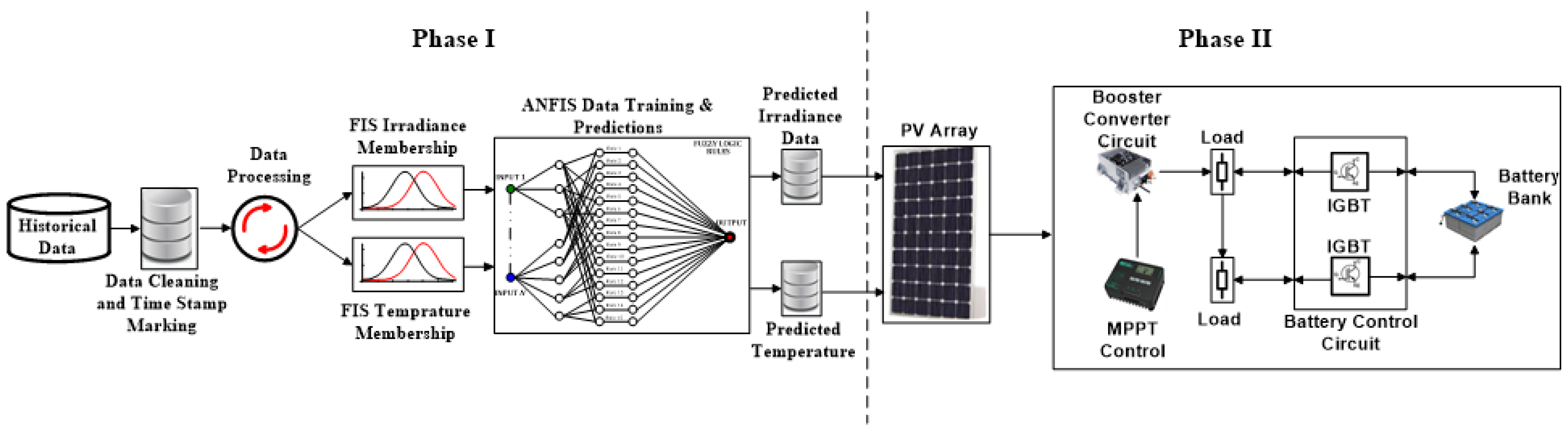
Figure 1.
Proposed ANFIS-based prediction and energy management framework.
Figure 1.
Proposed ANFIS-based prediction and energy management framework.
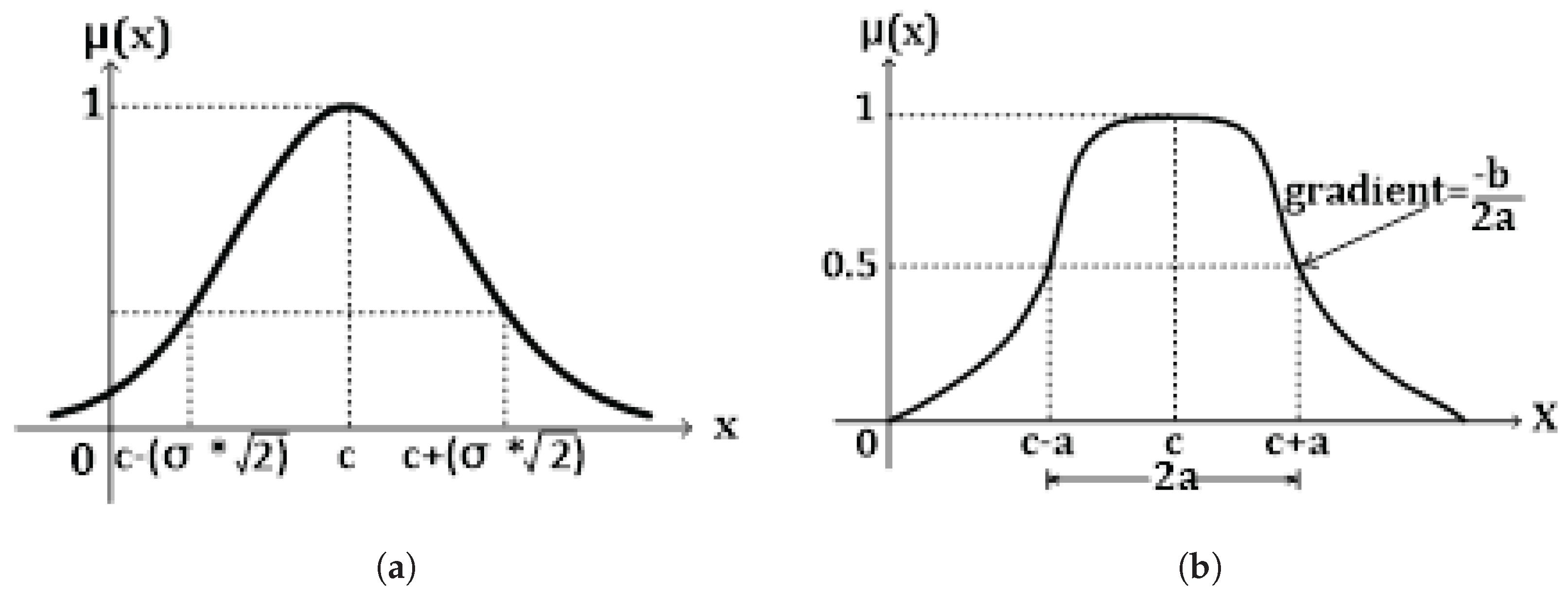
Figure 3.
Membership Functions: (a) Gaussian Function Member. (b) Generalized Bell Membership Function.
Figure 3.
Membership Functions: (a) Gaussian Function Member. (b) Generalized Bell Membership Function.
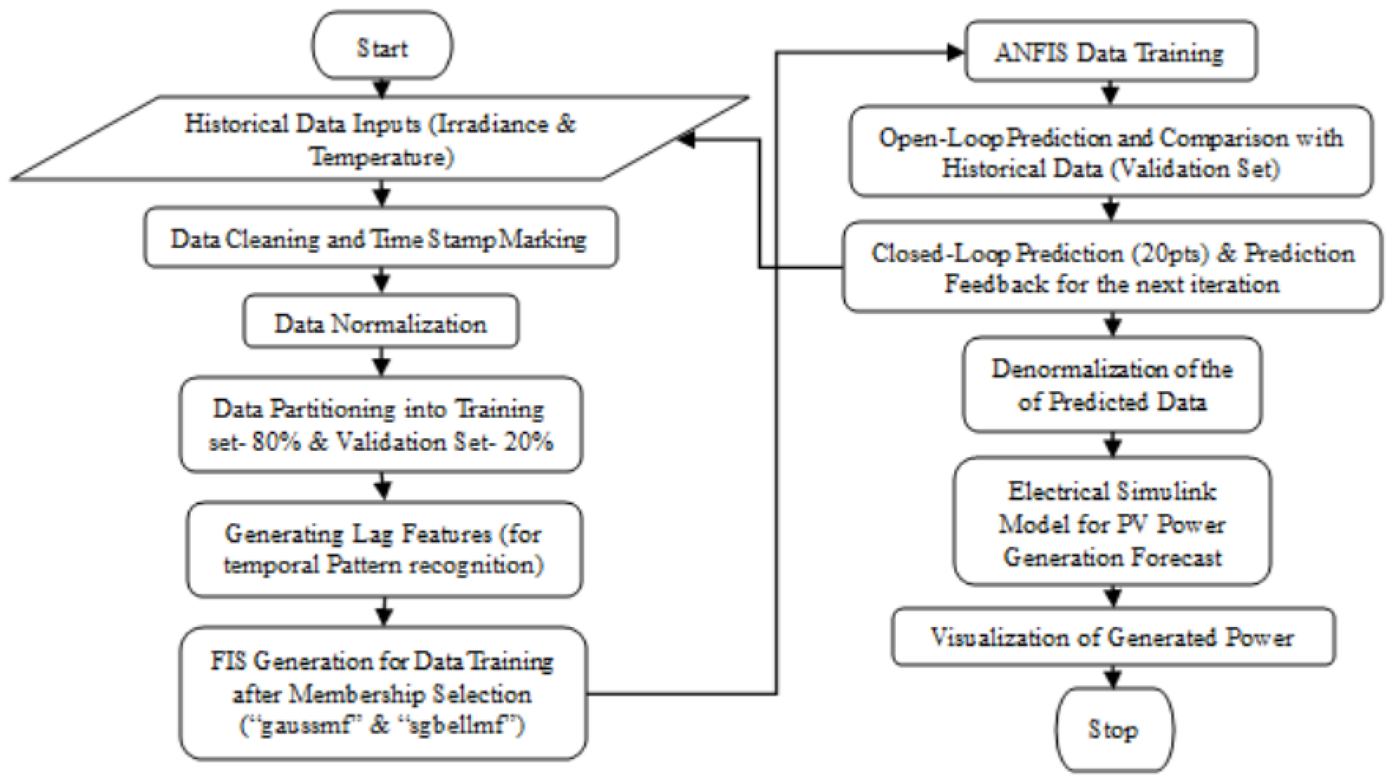
Figure 4.
Flowchart of the ANFIS training and prediction model.
Figure 4.
Flowchart of the ANFIS training and prediction model.
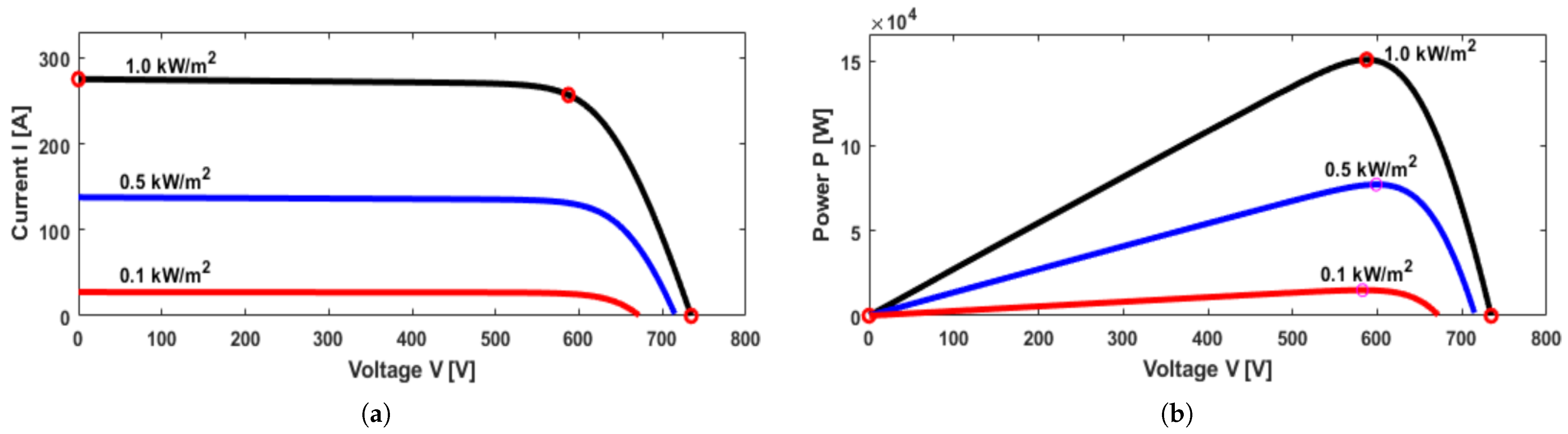
Figure 5.
Solar Farm PV-module characteristic curves: (a) I-V characteristic curve at 1, 0.5, and of irradiance. (b) P-V characteristic curve at 1, 0.5, and of irradiance.
Figure 5.
Solar Farm PV-module characteristic curves: (a) I-V characteristic curve at 1, 0.5, and of irradiance. (b) P-V characteristic curve at 1, 0.5, and of irradiance.
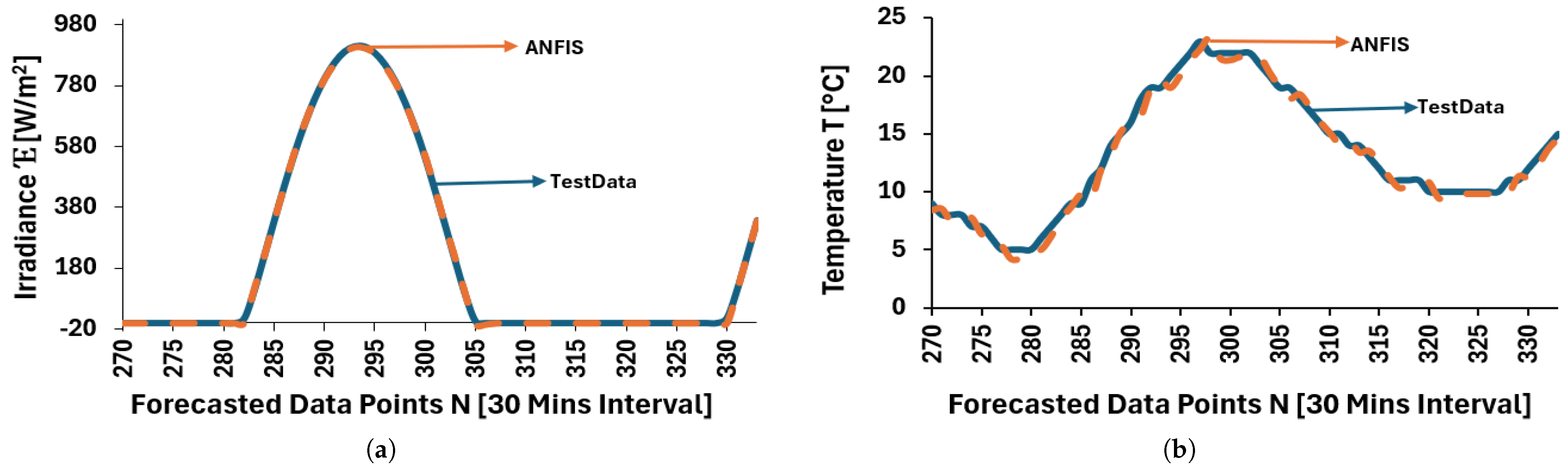
Figure 6.
Closed-Loop predictions using ANFIS: (a) test and predicted data— irradiance. (b) test and predicted data—temperature.
Figure 6.
Closed-Loop predictions using ANFIS: (a) test and predicted data— irradiance. (b) test and predicted data—temperature.
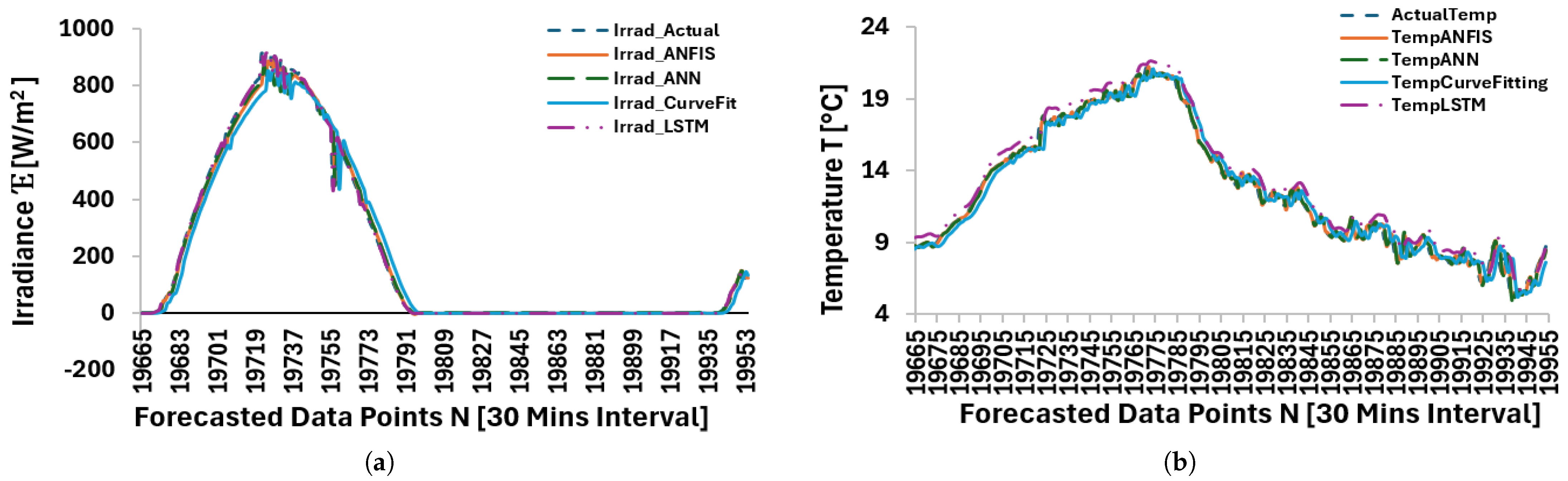
Figure 7.
Closed-loop predictions using ANFIS, ANN, CFiT, and LSTM: (a) test and predicted data—irradiance. (b) test and predicted data—temperature.
Figure 7.
Closed-loop predictions using ANFIS, ANN, CFiT, and LSTM: (a) test and predicted data—irradiance. (b) test and predicted data—temperature.
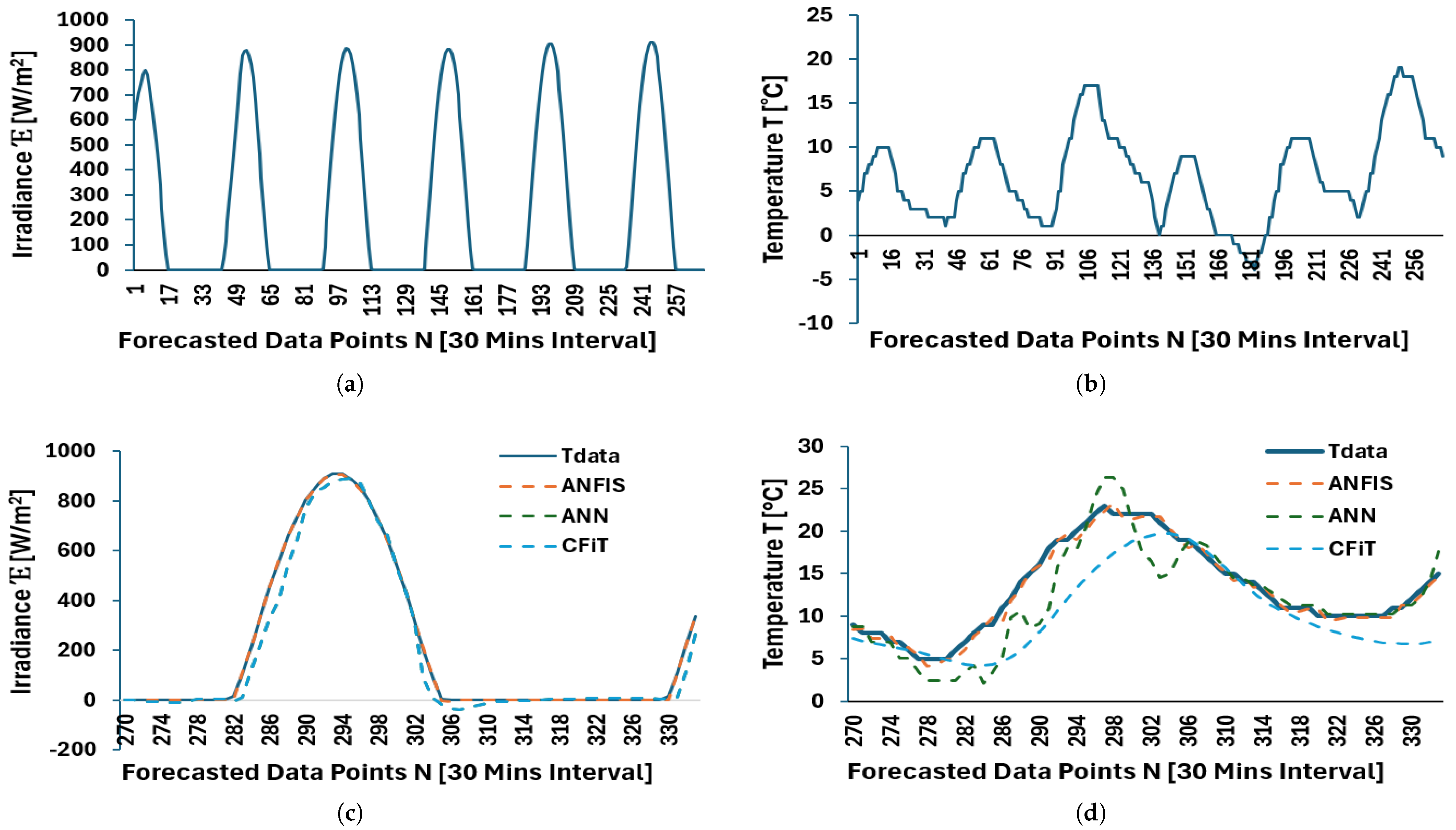
Figure 8.
Open-loop predictions using ANFIS, ANN, CFiT, and curve-fitting: (a) Historical data—irradiance. (b) Historical data—temperature. (c) Test and predicted data—irradiance. (d) Test and predicted data—temperature.
Figure 8.
Open-loop predictions using ANFIS, ANN, CFiT, and curve-fitting: (a) Historical data—irradiance. (b) Historical data—temperature. (c) Test and predicted data—irradiance. (d) Test and predicted data—temperature.
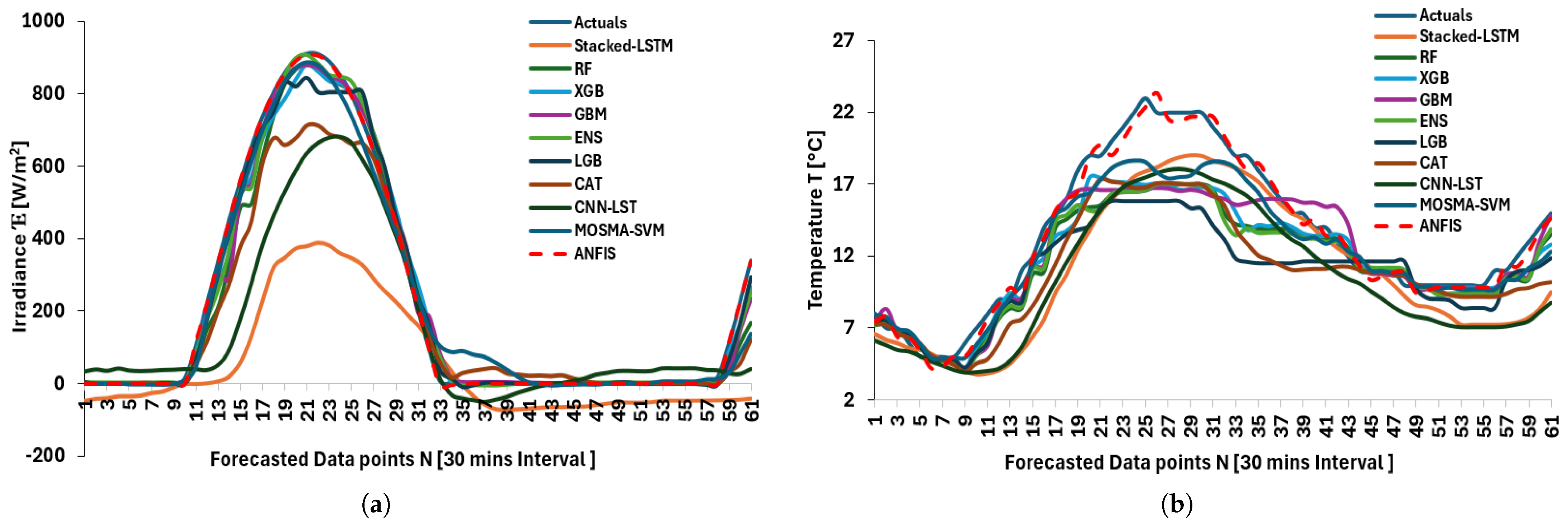
Figure 9.
Predictions using stacked LSTM, Random Forest, XGBoost, GBoostM, Transformer, individual/ensembles, LightGBM, CatBoost, CNN-LSTM, MOSMA-SVM, and ANFIS: (a) Forecasted data points—irradiance. (b) Forecasted data points—temperature. 62 observations forecasted.
Figure 9.
Predictions using stacked LSTM, Random Forest, XGBoost, GBoostM, Transformer, individual/ensembles, LightGBM, CatBoost, CNN-LSTM, MOSMA-SVM, and ANFIS: (a) Forecasted data points—irradiance. (b) Forecasted data points—temperature. 62 observations forecasted.
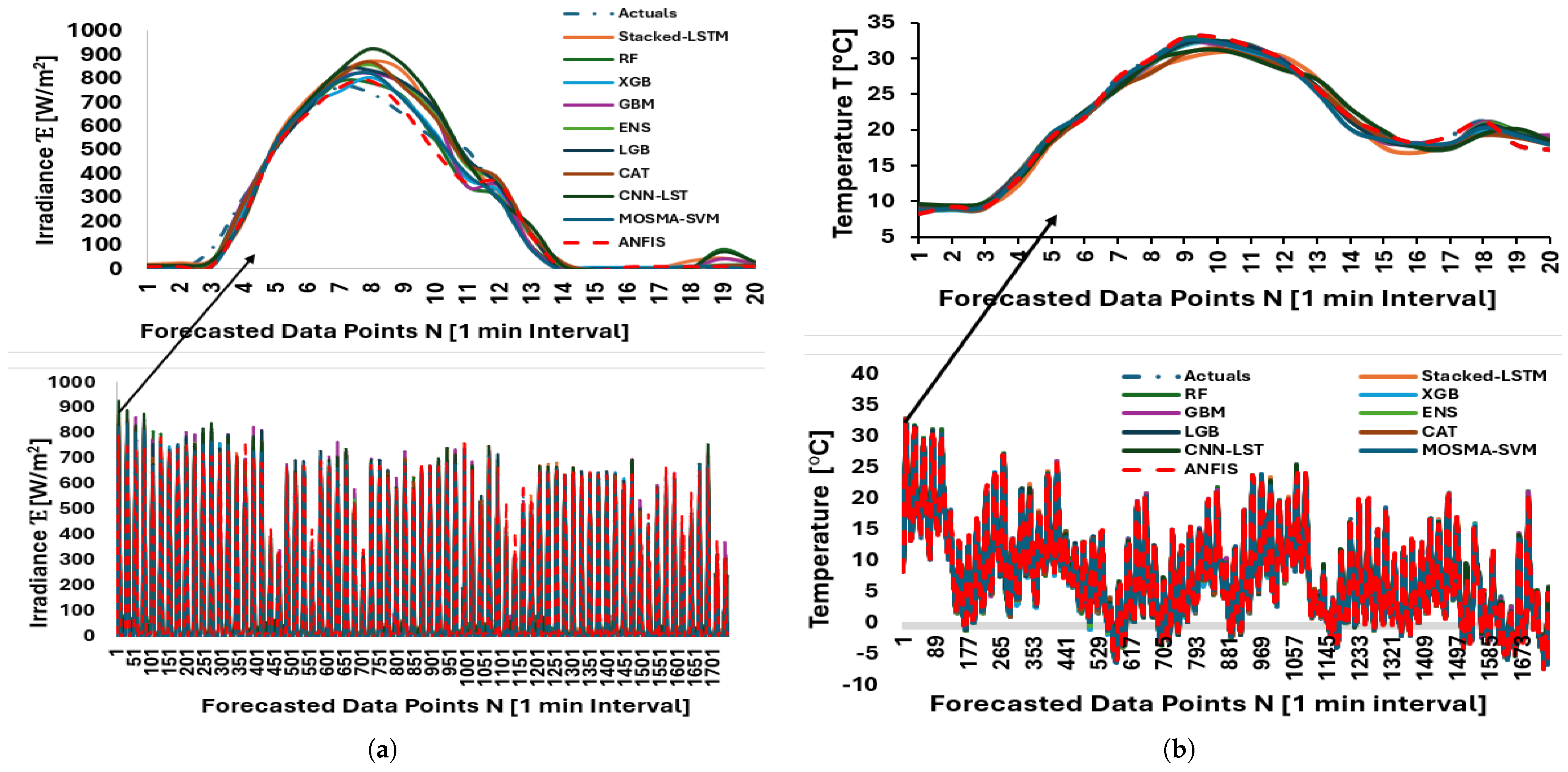
Figure 10.
Predictions using stacked LSTM, Random Forest, XGBoost, GBoostM, Transformer, individual/ensembles, LightGBM, CatBoost, CNN-LSTM, MOSMA-SVM, and ANFIS: (a) Forecasted data points—irradiance. (b) Forecasted data points—temperature. 1748 observations forecasted.
Figure 10.
Predictions using stacked LSTM, Random Forest, XGBoost, GBoostM, Transformer, individual/ensembles, LightGBM, CatBoost, CNN-LSTM, MOSMA-SVM, and ANFIS: (a) Forecasted data points—irradiance. (b) Forecasted data points—temperature. 1748 observations forecasted.
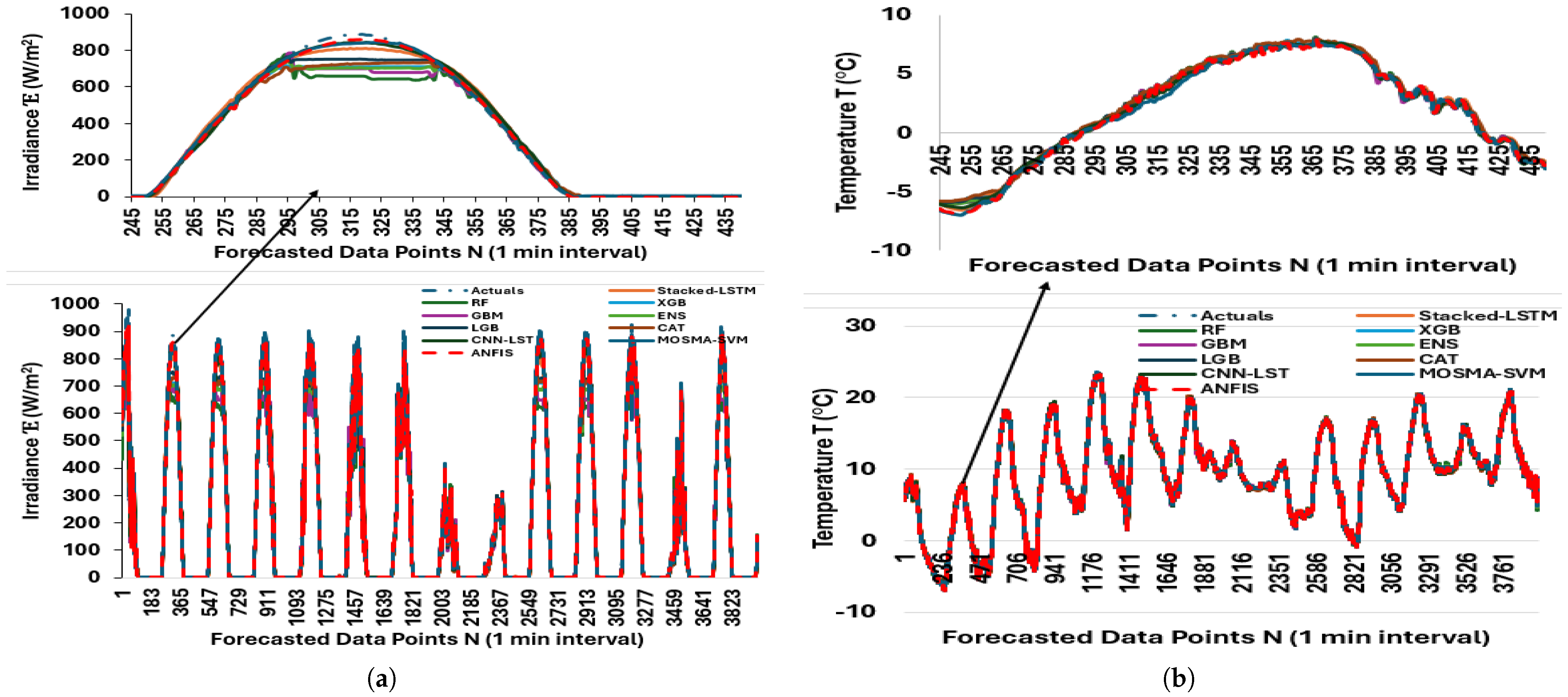
Figure 11.
Predictions using stacked LSTM, Random Forest, XGBoost, GBoostM, Transformer, individual/ensembles, LightGBM, CatBoost, CNN-LSTM, MOSMA-SVM, and ANFIS: (a) Forecasted data points—irradiance. (b) Forecasted data points—temperature. 3987 observations forecasted.
Figure 11.
Predictions using stacked LSTM, Random Forest, XGBoost, GBoostM, Transformer, individual/ensembles, LightGBM, CatBoost, CNN-LSTM, MOSMA-SVM, and ANFIS: (a) Forecasted data points—irradiance. (b) Forecasted data points—temperature. 3987 observations forecasted.
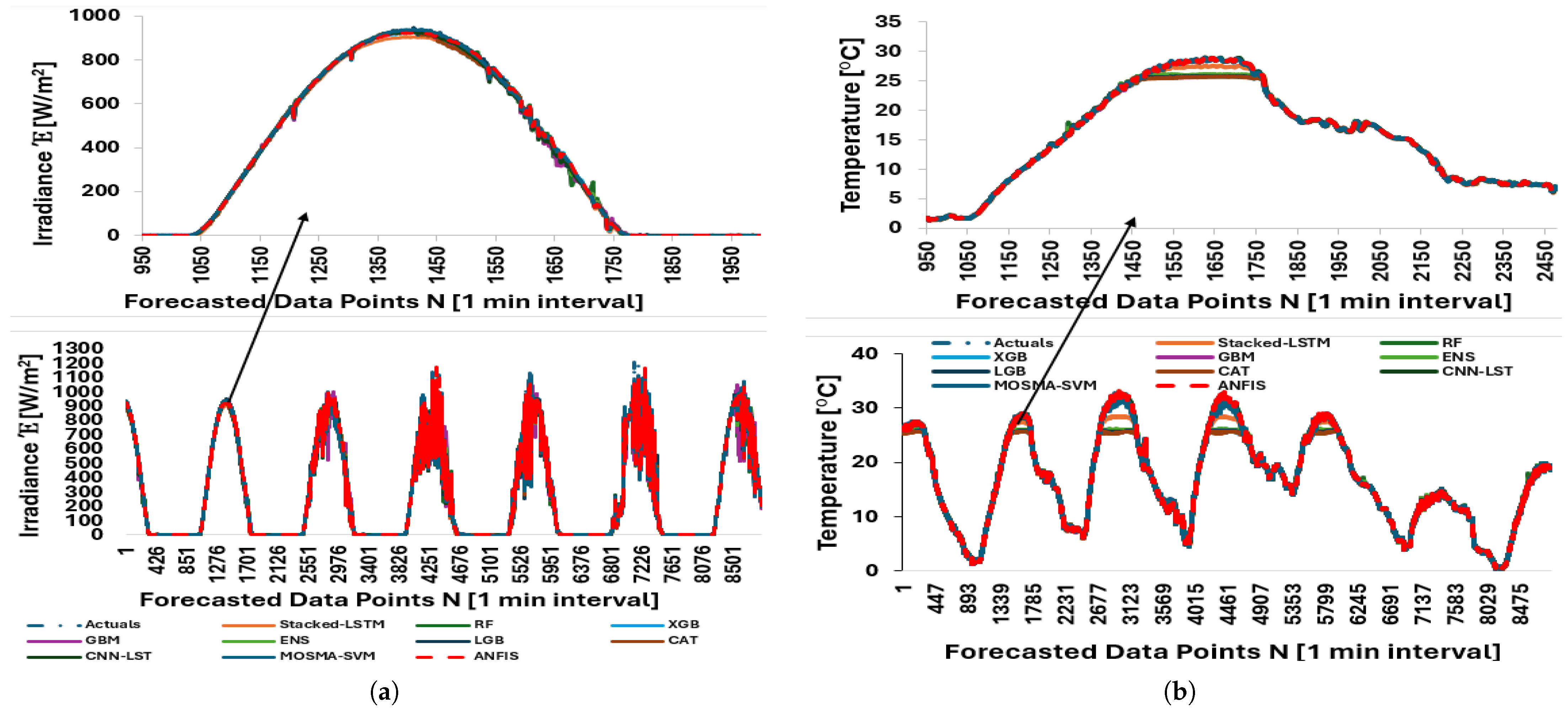
Figure 12.
Predictions using stacked LSTM, Random Forest, XGBoost, GBoostM, Transformer, individual/ensembles, LightGBM, CatBoost, CNN-LSTM, MOSMA-SVM, and ANFIS: (a) Forecasted data points—irradiance. (b) Forecasted data points—temperature. 8911 observations forecasted.
Figure 12.
Predictions using stacked LSTM, Random Forest, XGBoost, GBoostM, Transformer, individual/ensembles, LightGBM, CatBoost, CNN-LSTM, MOSMA-SVM, and ANFIS: (a) Forecasted data points—irradiance. (b) Forecasted data points—temperature. 8911 observations forecasted.
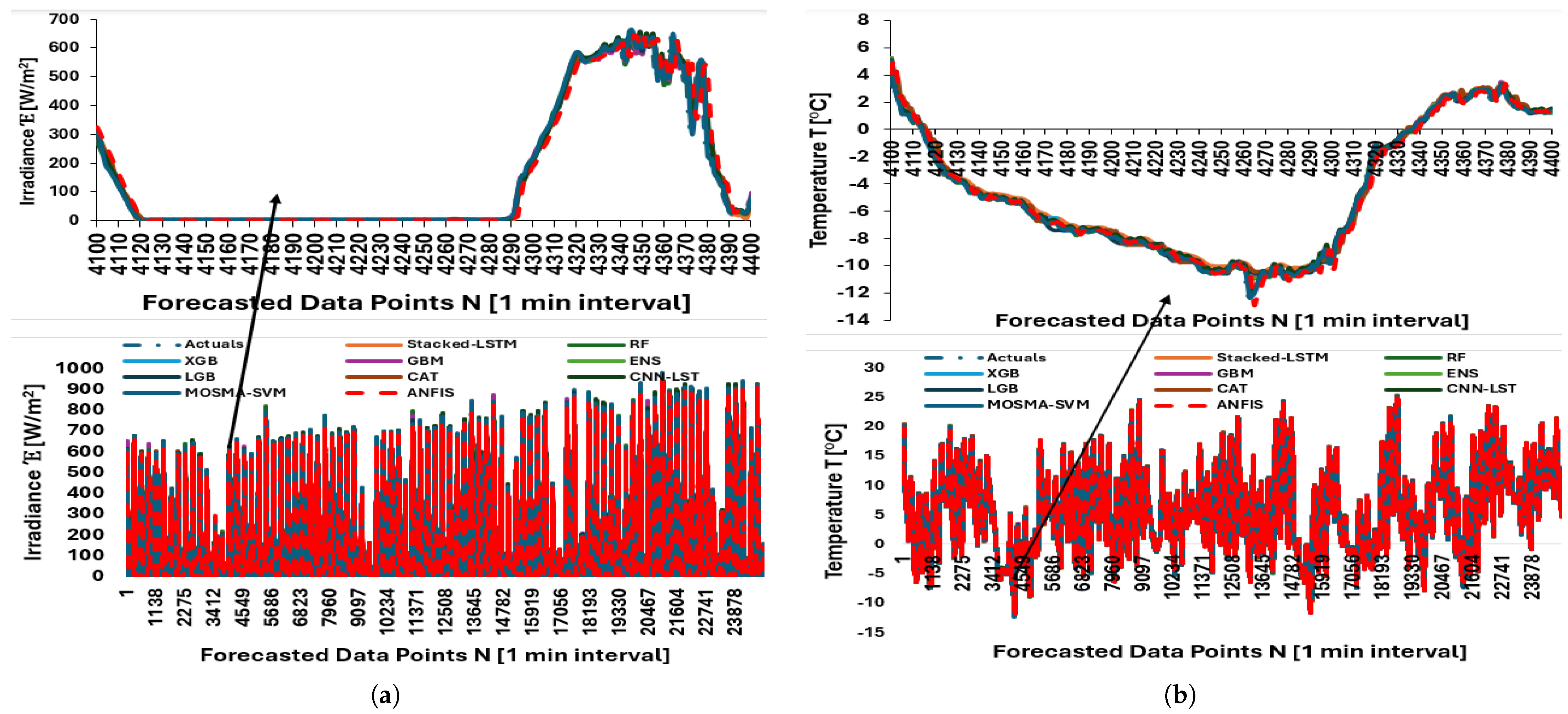
Figure 13.
Predictions using stacked LSTM, Random Forest, XGBoost, GBoostM, Transformer, individual/ensembles, LightGBM, CatBoost, CNN-LSTM, MOSMA-SVM, and ANFIS: (a) Forecasted data points—irradiance. (b) Forecasted data points—temperature. 25011 observations forecasted.
Figure 13.
Predictions using stacked LSTM, Random Forest, XGBoost, GBoostM, Transformer, individual/ensembles, LightGBM, CatBoost, CNN-LSTM, MOSMA-SVM, and ANFIS: (a) Forecasted data points—irradiance. (b) Forecasted data points—temperature. 25011 observations forecasted.
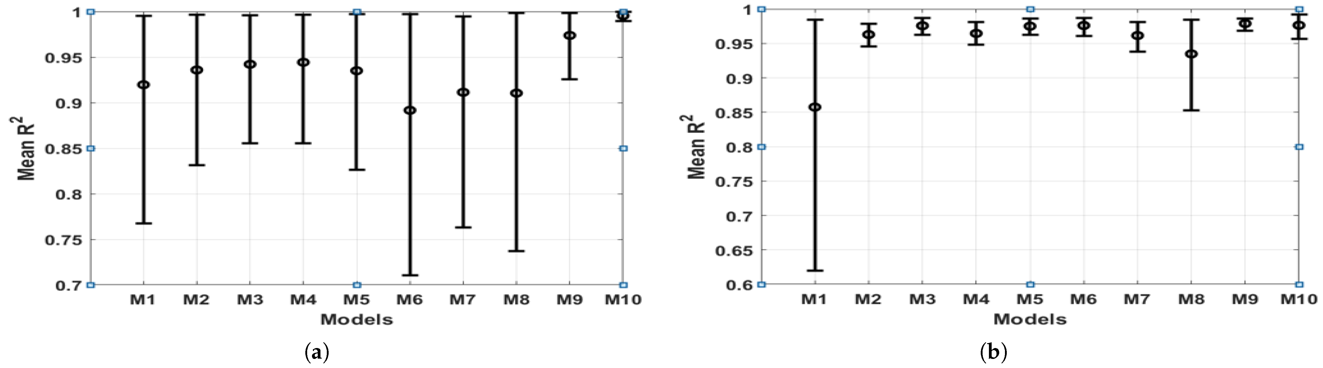
Figure 14.
Bootstrapped 95% confidence intervals of mean values: (a) Temperature . (b) Irradiance mean .
Figure 14.
Bootstrapped 95% confidence intervals of mean values: (a) Temperature . (b) Irradiance mean .
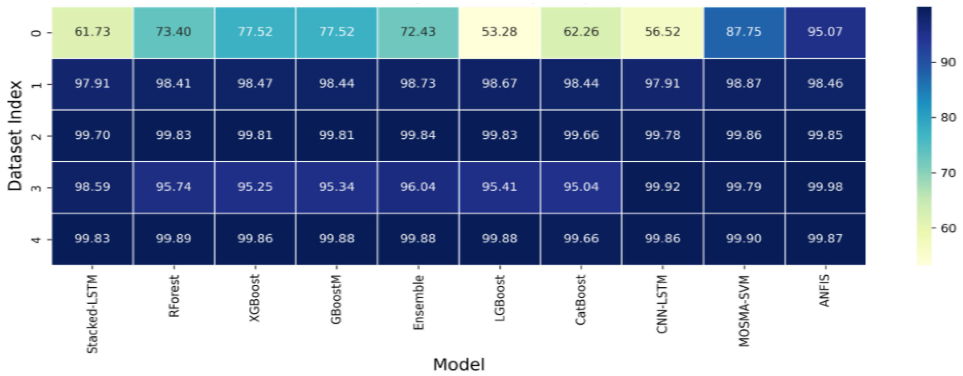
Figure 15.
score heatmap for temperature predictions as shown in
Table 5.
Figure 15.
score heatmap for temperature predictions as shown in
Table 5.
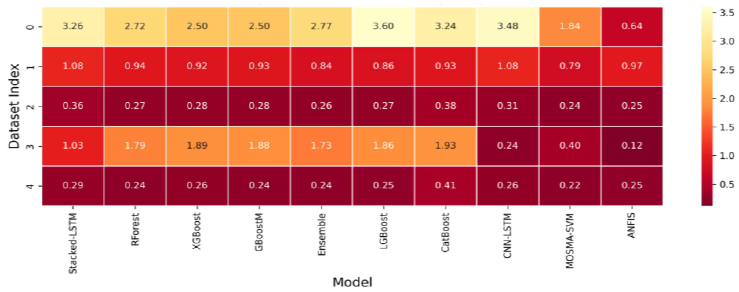
Figure 16.
heatmap for temperature predictions as shown in
Table 5.
Figure 16.
heatmap for temperature predictions as shown in
Table 5.
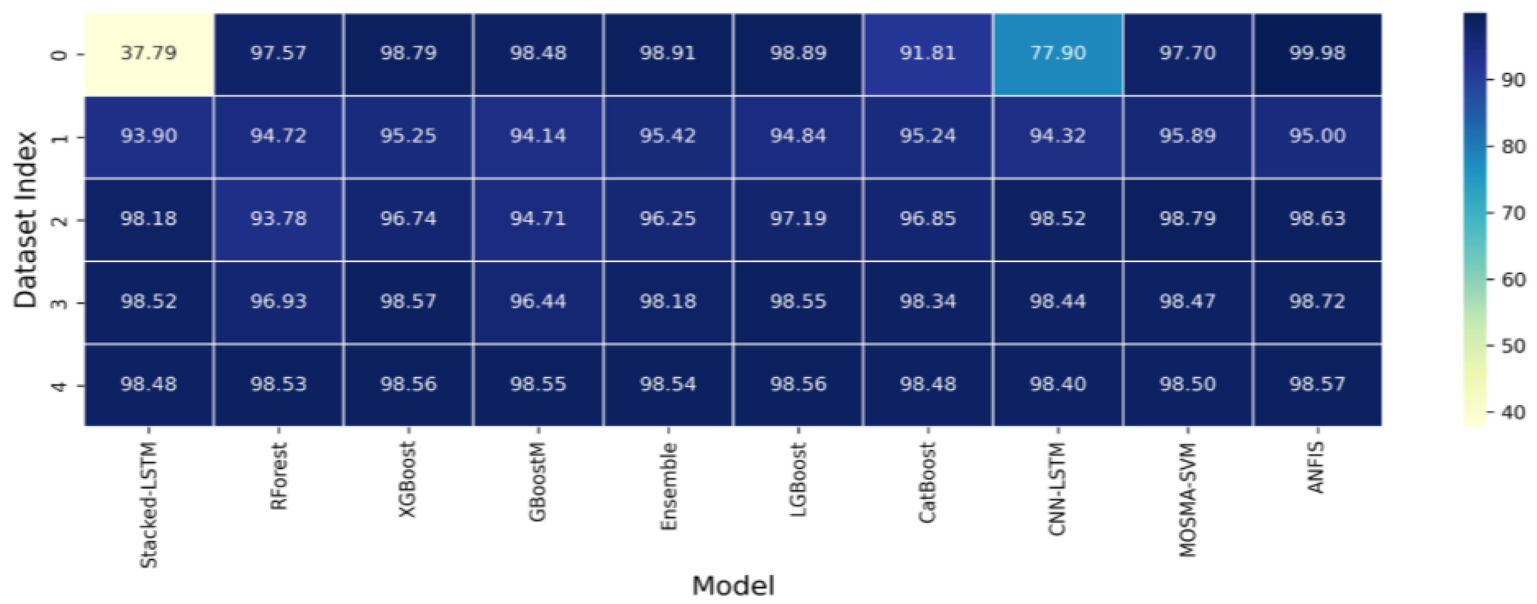
Figure 17.
score heatmap for irradiance predictions as shown in
Table 6.
Figure 17.
score heatmap for irradiance predictions as shown in
Table 6.
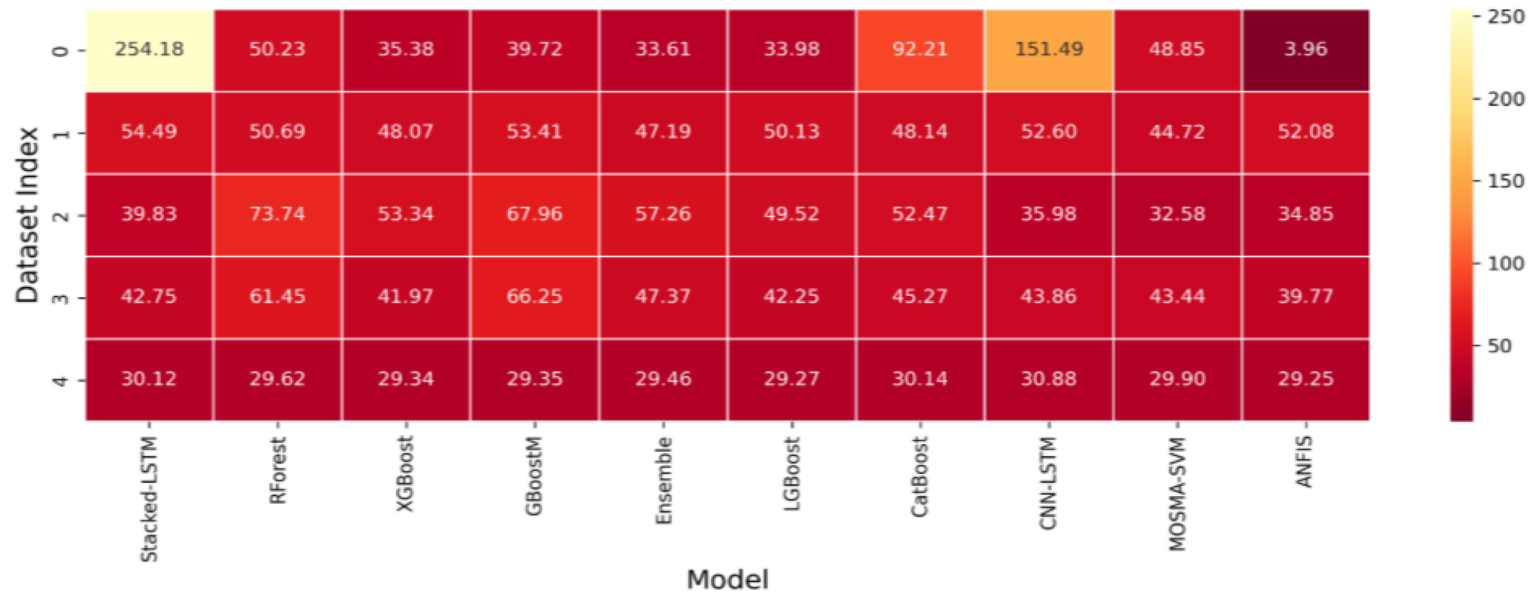
Figure 18.
heatmap for irradiance predictions as shown in
Table 6.
Figure 18.
heatmap for irradiance predictions as shown in
Table 6.
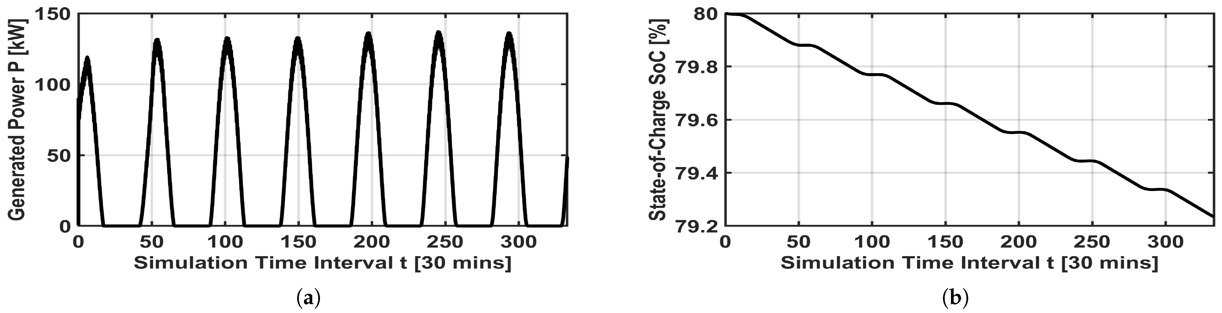
Figure 19.
Energy management: (a) PV-power generation for 7 consecutive days. (b) Nickel–cadmium battery State-of-Charge (SoC).
Figure 19.
Energy management: (a) PV-power generation for 7 consecutive days. (b) Nickel–cadmium battery State-of-Charge (SoC).
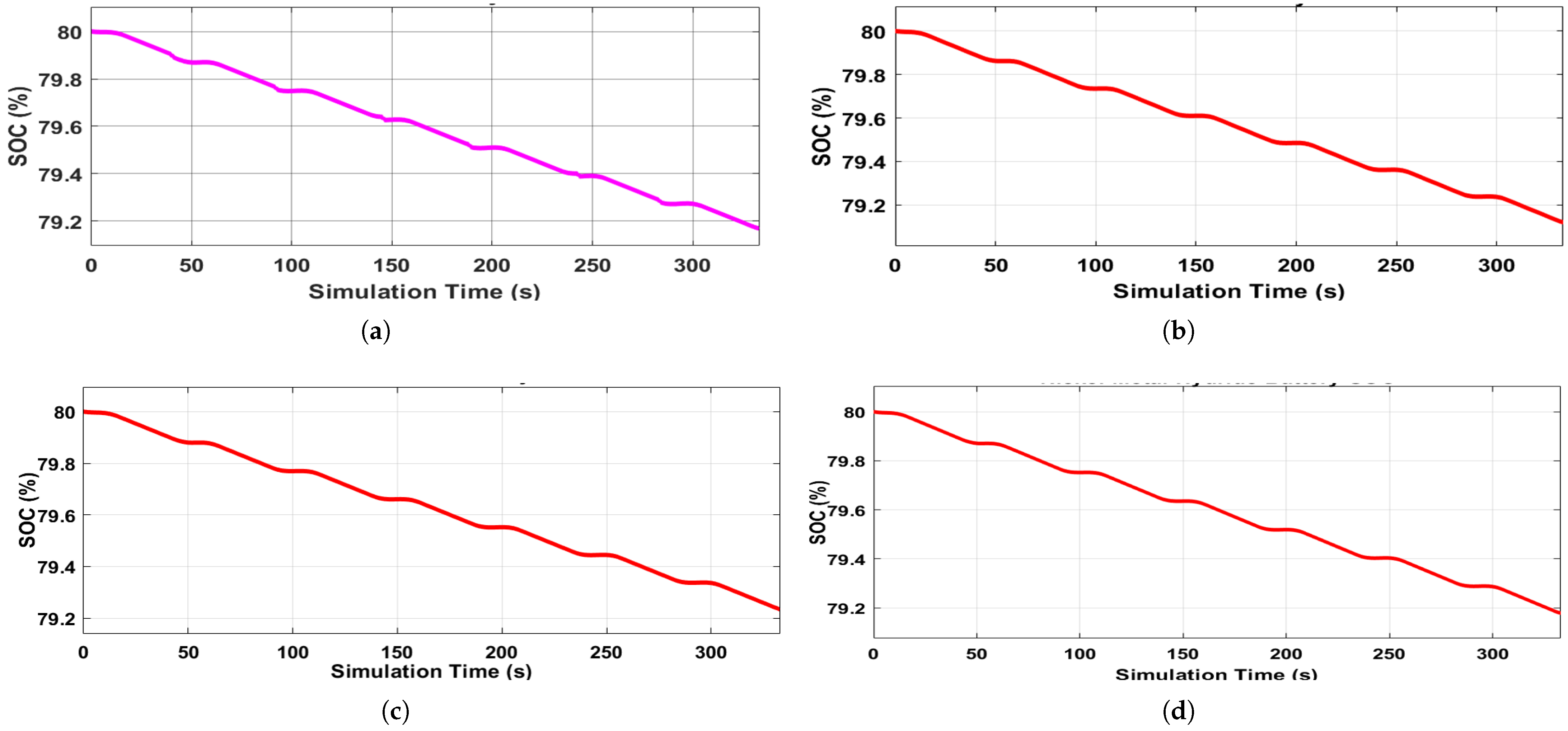
Figure 20.
Battery SoC plot using Data-1 on the model: (a) Lead acid battery SoC. (b) Lithium-ion battery SoC. (c) Nickel–cadmium battery SoC. (d) Nickel–metal–hydride battery SoC.
Figure 20.
Battery SoC plot using Data-1 on the model: (a) Lead acid battery SoC. (b) Lithium-ion battery SoC. (c) Nickel–cadmium battery SoC. (d) Nickel–metal–hydride battery SoC.
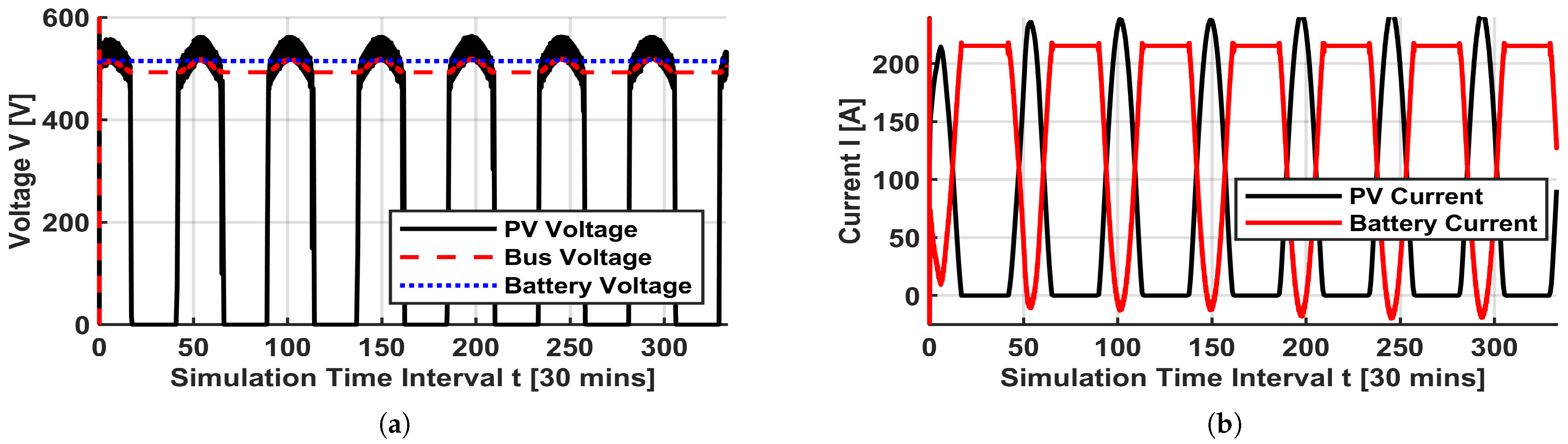
Figure 21.
Voltages and currents: (a) PV-array, bus, and battery voltages. (b) PV and battery current.
Figure 21.
Voltages and currents: (a) PV-array, bus, and battery voltages. (b) PV and battery current.
Table 1.
Prediction performance—accuracy/Root Mean Square Error (RMSE).
Table 1.
Prediction performance—accuracy/Root Mean Square Error (RMSE).
| S/N | Reference % | Title % | Achievement | Gap |
|---|
| 1 | [6,26] | PV Forecasting/Battery Management (Separate) | Forecasting and battery management performed separately | Lacks integration, leading to suboptimal SoC stability and energy use |
| 2 | [9,19] | Hybrid PV Prediction Models | Hybrid approach for PV forecasting | Struggles with fluctuating weather, reducing accuracy |
| 3 | [18,27] | CNN-LSTM for PV Forecasting | Improved accuracy in single-variable predictions | Cannot model multivariate dependencies, limiting efficiency |
| 4 | [24,25] | Single-Variable Prediction Models | Predicts one variable at a time | Lacks multivariate capability, reducing forecasting efficiency |
| 5 | [2,20] | ConvGNNs/MOSMA-SVM | High accuracy | Computationally intensive, limiting real-time use |
| 6 | [16] | Explainable AI (XAI) for Energy Systems | Uses external tools for interpretability | Requires additional tools for explanation |
| 7 | [7,28] | Forecasting-Focused Models | Effective energy prediction | Does not include battery control or load scheduling |
| 8 | [3,26] | PV Forecasting Under Extreme Conditions | Accurate in controlled settings | Struggles with complex weather without higher computation cost |
| 9 | ANFIS (Proposed) | Integrated PV Forecasting/Battery Management | Unifies PV forecasting and SoC management, ensuring stability and long battery autonomy. Uses MIMO for multivariate prediction, improving efficiency. Computationally lightweight, scalable, and explainable, making it ideal for real-world deployment. | Addresses key limitations, offering a holistic and interpretable solution. |
Table 2.
Dataset summary: size, sampling, forecast scope, and observed challenges.
Table 2.
Dataset summary: size, sampling, forecast scope, and observed challenges.
| S/N | Data Size | Sampling Interval | Forecast Data Size | Observed Challenges |
|---|
| 1 | 333 | 30 min | 62 | Outliers, poor data quality, environmental variability, and missing data |
| 2 | 8760 | 1 min | 1748 | Outliers due to data noise; high temporal and spatial variability |
| 3 | 19,954 | 1 min | 3987 | Poor data synchronization, time resolution issues, and missing data |
| 4 | 44,579 | 1 min | 8911 | Outliers, poor data quality, and missing data |
| 5 | 125,074 | 1 min | 25,011 | Long-term data gap, seasonality variations, and sensor maintenance issues |
Table 3.
Prediction performance—accuracy/Root Mean Square Error (RMSE).
Table 3.
Prediction performance—accuracy/Root Mean Square Error (RMSE).
| Method | Irradiance Accuracy % | Temperature Accuracy % | Irradiance RMSE | Temperature RMSE | Time (s) |
|---|
| ANN | 83.01 | 97.27 | 33.94 | 0.25 | 159 |
| Curve-Fit | 73.15 | 93.77 | 53.64 | 0.58 | 224 |
| LSTM | 80.14 | 72.87 | 50.55 | 0.75 | 371 |
| ANFIS | 84.55 | 97.27 | 32.85 | 0.25 | 58 |
Table 4.
Prediction performance—accuracy/Root Mean Square Error (RMSE).
Table 4.
Prediction performance—accuracy/Root Mean Square Error (RMSE).
| Method | Irradiance Accuracy % | Temperature Accuracy % | Irradiance RMSE | Temperature RMSE |
|---|
| ANN | 78.25 | 63.55 | 33.87 | 34.98 |
| Curve-Fitting | 72.3 | 64.3 | 27.24 | 29.56 |
| ANFIS | 98.17 | 95.10 | 3.72 | 0.64 |
Table 5.
Temperature prediction performance: score (%) and Root Mean Square Error (RMSE).
Table 5.
Temperature prediction performance: score (%) and Root Mean Square Error (RMSE).
| S/N | Stacked-LSTM | RForest | XGBoost | GBoostM | Ensemble | LGBoost | CatBoost | CNN-LSTM | MOSMA-SVM | ANFIS | Data Length—Forecast |
|---|
| R2-Score (Accuracy %) |
| 1 | 61.73 | 73.40 | 77.52 | 77.52 | 72.43 | 53.28 | 62.26 | 56.52 | 87.75 | 95.07 | 62 |
| 2 | 97.91 | 98.41 | 98.47 | 98.44 | 98.73 | 98.67 | 98.44 | 97.91 | 98.87 | 98.46 | 1748 |
| 3 | 99.70 | 99.83 | 99.81 | 99.81 | 99.84 | 99.83 | 99.66 | 99.78 | 99.86 | 99.85 | 3987 |
| 4 | 98.59 | 95.74 | 95.25 | 95.34 | 96.04 | 95.41 | 95.04 | 99.92 | 99.79 | 99.98 | 8911 |
| 5 | 99.83 | 99.89 | 99.86 | 99.88 | 99.88 | 99.88 | 99.66 | 99.86 | 99.90 | 99.87 | 25,011 |
| Avg | 91.55 | 93.45 | 94.18 | 94.20 | 93.39 | 89.41 | 91.01 | 90.80 | 97.24 | 98.65 | – |
| RMSE |
| 1 | 3.26 | 2.72 | 2.50 | 2.50 | 2.77 | 3.60 | 3.24 | 3.48 | 1.84 | 0.64 | 62 |
| 2 | 1.08 | 0.94 | 0.92 | 0.93 | 0.84 | 0.86 | 0.93 | 1.08 | 0.79 | 0.97 | 1748 |
| 3 | 0.36 | 0.27 | 0.28 | 0.28 | 0.26 | 0.27 | 0.38 | 0.31 | 0.24 | 0.25 | 3987 |
| 4 | 1.03 | 1.79 | 1.89 | 1.88 | 1.73 | 1.86 | 1.93 | 0.24 | 0.40 | 0.12 | 8911 |
| 5 | 0.29 | 0.24 | 0.26 | 0.24 | 0.24 | 0.25 | 0.41 | 0.26 | 0.22 | 0.25 | 25,011 |
| Avg | 1.20 | 1.19 | 1.17 | 1.17 | 1.17 | 1.37 | 1.38 | 1.07 | 0.70 | 0.45 | – |
Table 6.
Irradiance prediction performance: score (%) and Root Mean Square Error (RMSE).
Table 6.
Irradiance prediction performance: score (%) and Root Mean Square Error (RMSE).
| S/N | Stacked-LSTM | RForest | XGBoost | GBoostM | Ensemble | LGBoost | CatBoost | CNN-LSTM | MOSMA-SVM | ANFIS | Data Length—Forecast |
|---|
| Score (%) |
| 1 | 37.79 | 97.57 | 98.79 | 98.48 | 98.91 | 98.89 | 91.81 | 77.90 | 97.70 | 99.98 | 62 |
| 2 | 93.90 | 94.72 | 95.25 | 94.14 | 95.42 | 94.84 | 95.24 | 94.32 | 95.89 | 95.00 | 1748 |
| 3 | 98.18 | 93.78 | 96.74 | 94.71 | 96.25 | 97.19 | 96.85 | 98.52 | 98.79 | 98.63 | 3987 |
| 4 | 98.52 | 96.93 | 98.57 | 96.44 | 98.18 | 98.55 | 98.34 | 98.44 | 98.47 | 98.72 | 8911 |
| 5 | 98.48 | 98.53 | 98.56 | 98.55 | 98.54 | 98.56 | 98.48 | 98.40 | 98.50 | 98.57 | 25,011 |
| Avg | 85.37 | 96.31 | 97.58 | 96.47 | 97.46 | 97.61 | 96.14 | 93.51 | 97.87 | 98.18 | – |
| RMSE |
| 1 | 254.18 | 50.23 | 35.38 | 39.72 | 33.61 | 33.98 | 92.21 | 151.49 | 48.85 | 3.96 | 62 |
| 2 | 54.49 | 50.69 | 48.07 | 53.41 | 47.19 | 50.13 | 48.14 | 52.60 | 44.72 | 52.08 | 1748 |
| 3 | 39.83 | 73.74 | 53.34 | 67.96 | 57.26 | 49.52 | 52.47 | 35.98 | 32.58 | 34.85 | 3987 |
| 4 | 42.75 | 61.45 | 41.97 | 66.25 | 47.37 | 42.25 | 45.27 | 43.86 | 43.44 | 39.77 | 8911 |
| 5 | 30.12 | 29.62 | 29.34 | 29.35 | 29.46 | 29.27 | 30.14 | 30.88 | 29.90 | 29.25 | 25,011 |
| Avg | 84.27 | 53.14 | 41.62 | 51.34 | 42.98 | 41.03 | 53.65 | 62.96 | 39.90 | 31.98 | – |
Table 7.
Model computational time—temperature and irradiance.
Table 7.
Model computational time—temperature and irradiance.
| S/N | Stacked-LSTM | RForest | XGBoost | GBoostM | Ensemble | LGBoost | CatBoost | CNN-LSTM | MOSMA-SVM | ANFIS | Data Length—Forecast |
|---|
| 1 | 125.68 | 1.01 | 15.24 | 3.19 | 9.71 | 14.81 | 13.76 | 35.42 | 0.04 | 0.25 | 62 |
| 2 | 431.99 | 6.34 | 11.91 | 17.56 | 35.20 | 34.09 | 34.62 | 151.26 | 20.31 | 4.03 | 1748 |
| 3 | 901.81 | 30.91 | 18.56 | 52.44 | 104.55 | 104.19 | 106.26 | 306.06 | 58.61 | 9.06 | 3987 |
| 4 | 2012.62 | 64.30 | 24.55 | 114.67 | 208.89 | 211.53 | 204.89 | 624.81 | 146.07 | 20.03 | 8911 |
| 5 | 4747.04 | 243.32 | 58.88 | 310.71 | 569.46 | 552.50 | 556.30 | 1784.19 | 5917.97 | 56.58 | 25011 |
| Avg | 1643.83 | 69.17 | 25.83 | 99.71 | 185.56 | 183.42 | 183.17 | 580.35 | 1228.60 | 17.99 | – |
Table 8.
SoC summary table in descending order.
Table 8.
SoC summary table in descending order.
| S/N | Battery Type | SoC (%) |
|---|
| 1 | Nickel–cadmium | 79.24 |
| 2 | Nickel–metal–hydride | 79.18 |
| 3 | Lead acid | 79.17 |
| 4 | Lithium ion | 79.12 |


 ,
, 
