Article

Modeling Cost-Effectiveness of Photovoltaic Module Replacement Based on Quantitative Assessment of Defect Power Loss

by
Victoria Lofstad-Lie
1,*,
Bjørn Lupton Aarseth
2,
Nathan Roosloot
1,2,
Erik Stensrud Marstein
1,2 and
Torbjørn Skauli
1,3
1
Department of Technology Systems, University of Oslo, 2007 Kjeller, Norway
2
Institute for Energy Technology (IFE), 2007 Kjeller, Norway
3
Norwegian Defence Research Establishment, 2007 Kjeller, Norway
*
Author to whom correspondence should be addressed.
Solar 2024, 4(4), 728-743; https://doi.org/10.3390/solar4040034
Submission received: 3 October 2024 / Revised: 22 November 2024 / Accepted: 11 December 2024 / Published: 19 December 2024

Abstract

The degradation of solar photovoltaic (PV) modules over time, which are aggravated by defects, significantly affects the performance of utility-scale PV parks. This study presents a quantitative assessment of the power loss from module defects and evaluates the cost-effectiveness of replacing defective modules at various stages of degradation. A module test site was established in Norway with six different defects, and continuous thermographic monitoring, combined with light IV measurements and electroluminescence (EL) imaging, provides partial support for further calculations on the long-term effects of the defects. The cumulative module energy loss is calculated over a 25-year park lifespan under both Norwegian and Chilean environmental conditions, with the latter representing higher solar irradiation levels. The energy gain from replacing the defective modules at various stages of degradation is compared to the costs of replacement, both for infant-life failures and mid-life failures. It is likely not beneficial to replace minor infant-life defects of 1% power loss in low-irradiation regions like Norway. For Chilean conditions, it can be cost-effective, but primarily if the module is replaced around mid park life, which gives a larger yield when replaced with a new module. For more severe defects of 10% loss, the replacement gain is above the replacement cost for high-irradiation locations, and replacing the 33% power loss defect is cost-effective for both locations, even when discovered late in the park lifetime. It is primarily beneficial to replace mid-life defects in high-irradiation locations.

1. Introduction

Solar photovoltaic (PV) technology has become one of the leading renewable energy resources due to technological advancements and a significant reduction in power generation costs [1]. Between 2010 and 2022, the global average cost of electricity generation from large-scale PV plants decreased by nearly 89% [2]. However, as PV systems age, the degradation of modules and the emergence of defects become critical factors that affect their long-term performance, reliability, and economic viability [3].
Module defects, such as hot spots, cracks, or defective bypass diodes, can lead to considerable power losses over time, which reduce the overall efficiency of the system [4]. Detecting these defects and quantifying their impact on power output is essential for effective operation and maintenance (O&M) strategies. Module defects are typically detected with aerial thermography, which offers a rapid method for the classification of different defect modes based on the thermal signature [5,6,7]. Accurate defect identification allows operators to make informed decisions about when to repair or replace defective modules, thus ensuring maximum energy yield and return on investment (ROI). A cost-based failure modes and effects analysis (FMEA) has been proposed for PV systems to evaluate O&M actions like module replacement or repair [8,9,10]. By calculating a cost priority number (CPN), different failure modes can be ranked based on their economic impact. This approach enables cost-based prioritization in O&M strategies, improving overall efficiency.
This paper presents a quantitative assessment of power losses due to defects in PV modules, focusing on the cost-effectiveness of module replacement. The study was initiated as an experiment where a module test site was established, and the modules were characterized during lab tests and with thermography. The measurements from the module test site form the foundation for further calculations on the cumulative power loss during a 25-year park life, taking into account a general module degradation, as well as a deterioration of the defects. Finally, the energy gain associated with replacing defective modules is presented at different stages of degradation, both for defects appearing early in the park’s lifespan and defects appearing mid-life. The study examines how environmental factors, such as solar irradiation, influence the defect loss, comparing results from the test site in Norway with simulated conditions in Chile. Norway represents a region of low solar irradiance, while Chile exemplifies a high-irradiation area. The two locations define the boundaries of solar irradiance conditions and effectively capture the range of variation. The energy gain is compared to the cost of replacing the modules, which determines if and when replacement is the cost-effective O&M measure.

2. Module Degradation—A Brief Review

Module degradation refers to a gradual decline in performance while still meeting the warranty requirements [11]. Examples of degradation modes are encapsulant discoloration, delamination, and ribbon discoloration. Environmental factors, such as high UV irradiation, humidity, and temperature, have been identified as significant contributors to the degradation process [12]. Studies describe higher degradation rates in hotter climates compared to more moderate climates [13,14]. In [15], the authors explore the degradation rates in four climate zones based on the Köppen–Geiger classification and find a median degradation rate of around 0.9% in desert climate, 0.5% in hot and humid climate, 0.7% in moderate climate, and 0.5% in climates with snow.
In addition to the gradual module degradation from exposure to the elements, it has been reported that defects might deteriorate with time, causing an additional degradation of defective modules [16]. In [17], the authors find that modules with cracked cells degraded in the field with an average of 0.5% more than uncracked modules over a period of 21 months, which corresponds to a yearly additional degradation of 0.3% for the cracked modules. The authors in [18] compare the degradation rates of 60 healthy modules with 40 modules with hotspots operating over 10–17 years in a desert climatic condition of Arizona. In the absence of intermittent performance data on the individual modules, the degradation rate is assumed to be linear, yielding an increase in the degradation rate of 0.46–3.3% per year in the modules with hotspots compared to the non-defective modules for different models. On average, the 35 defective p-Si modules in the experiment had an elevated degradation of 0.8% compared to the non-defective. While most studies conducted on the degradation of defective modules typically assume a linear degradation rate, the authors in [19] suggest that the fault degradation might follow other curves than a linear degradation. A module exhibiting cracks in the cell and the string interconnect ribbons degraded 12% over a period of ten years, following a curve shown in Figure A1 in Appendix A. The authors found a degradation following the exponential function y(t) = 0.181 · (1.055t− 1), where t is time in years. The defect degradation is not compared to the non-defective module degradation, so in further analyses, the exponential function will represent the total degradation. Ref. [20] found no evolution of cracks after one year of outdoor exposure.
In this article, we will differentiate between module degradation and defect degradation and treat them as additive effects. We will refer to module degradation as the median degradation exhibited by all PV modules in the power plant and defect degradation as the additional degradation exhibited by PV modules with observed defects. The analyses will explore the energy loss from defective modules located in Norway and Chile. Norway falls in the “snow” climate in [15], so a module degradation of 0.5% will be used, while Chile classifies as “desert” climate, with the associated median degradation rate of 0.9%. The module degradation and defect degradation in the mentioned literature are summarized in Figure 1 for the following: (a) Norway; (b) Chile. As with the module degradation, the defect degradation rate might also depend on the climatic zone. However, a lack of publications on the topic limits this study to assuming the same defect degradation in Norway and Chile.

3. Experimental Section

A module test site with six defective c-Si modules, as well as two reference modules, was established at Kjeller ( 60 ° N), Norway, for continuous thermographic monitoring and periodic lab characterization. The module setup is shown in infrared in Figure 2. The modules named Park defects 1 and 2 have cell hotspots that were discovered during operational monitoring. The modules were produced in 2012, and are collected from Glava Energy Center in Sweden. The module named Controlled defects 1–4 have defects deliberately created by the authors. Controlled defect 1 has an open-circuit substring resulting from cutting the connection to one of the cell strings, which is equivalent to a situation where the bypass diode is activated. A reference module of the same type is shown as Ref. 1. Controlled defects 2–4 have cell cracks that were created by damaging selected cells using a hammer on the backside of the module and imitate failures caused by mechanical stress or manufacturing issues. The corresponding reference module is denoted as Ref. 2. All the modules are connected in series, but with individual optimizers, meaning that each module operates at its maximum power point independently of each other.
All modules were characterized with light IV measurements on 26 August 2020. The measurements were performed with a Spi-Sun 5100 Single Long Pulse (SLP) solar simulator with an A+A+A+ rating according to [21], and a repeatability of 0.3%. Light IV is used to measure electrical properties like the maximum power Pmax at standard test conditions (STC) of 1000 W/m2. Additionally, electroluminescence (EL) imaging of the modules was performed on the same day with a custom-built setup using a Nikon D850 DSLR 45.7 MP camera with a Zeiss ZF-IR 1.4/85 lens. Images were taken according to IEC standard [22]. For Controlled defects 1–4, the light IV measurements and electroluminescence imaging were performed before and after the damage was inflicted on the modules to assess the effect of the defects.
A Flir A325 radiometric thermal camera with a resolution of 320 × 240 pixels was permanently installed on an adjacent rooftop. The camera has a field of view of 25° × 18.8°, a spectral range of 7.5 to 13.0 µm, and a thermal sensitivity of 70 mK at 30 °C. The camera imaged the module test site every minute during the following time intervals:
  • 2020: 27 August to 9 September, 1 to 8 October;
  • 2021: 5 May to 9 September;
  • 2022: 19 May to 8 June.
Additionally, the solar irradiance was measured in the module plane every five minutes using a silicon irradiance sensor from IMT Technology with an accuracy of ±5 W/m2 ± 2.5% of the read-out value.

4. Methodology

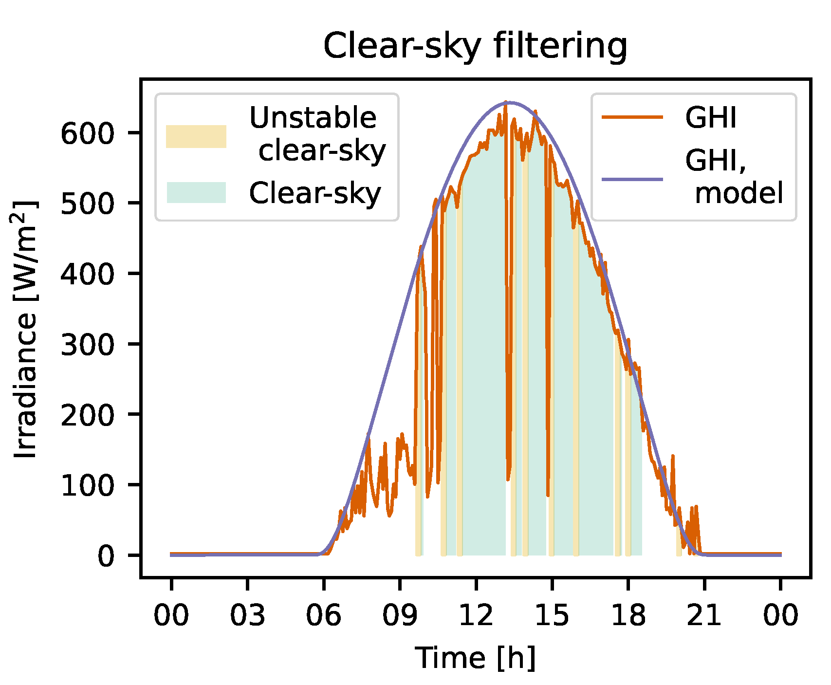
4.1. Clear-Sky Filtering of Thermography Images

Photovoltaic Library (PVLIB) [23] was used to model the clear-sky Global Horizontal Irradiance (GHI) at the solar array’s location, which was compared to the irradiation measured on-site. Clear-sky conditions were determined when the deviation between the measurements and the model was below 10%. This threshold value was determined from manual testing and inspection. Additionally, to achieve steady-state conditions, a continuous duration of clear-sky conditions for at least 10 min was required. Only periods of clear-sky and steady-state conditions are used for the thermography analysis. Figure 3 illustrates the filtering, where the modeled and measured GHIs are in purple and red, respectively. The green areas indicated clear-sky and steady-state conditions, while the yellow areas indicated that clear-sky conditions are met, but a thermal steady-state is not yet achieved.

4.2. Defect Heating and Power Loss

The temperature difference between a defect and a healthy module is denoted Δ T and represents a key parameter to determine the type and severity of a defect from thermal images. In steady-state conditions, Δ T acts as proportional to the power loss Δ P caused by internal defects in a module, as dictated by the energy balance, where the additional internal losses are dissipated as heat in accordance with the conservation of energy [24]. With Δ T as the temperature difference between a defective and non-defective module, this can be expressed as
Δ T = k · Δ P
where k is the proportionality constant. Due to the low lateral thermal conductivity of a module, the heating tends to be localized to the defective cells. It then follows that the temperature difference Δ Tcell between the defective cells and the non-defective area is
Δ T cell · A = k · Δ P
where A is the area of the defective cells.

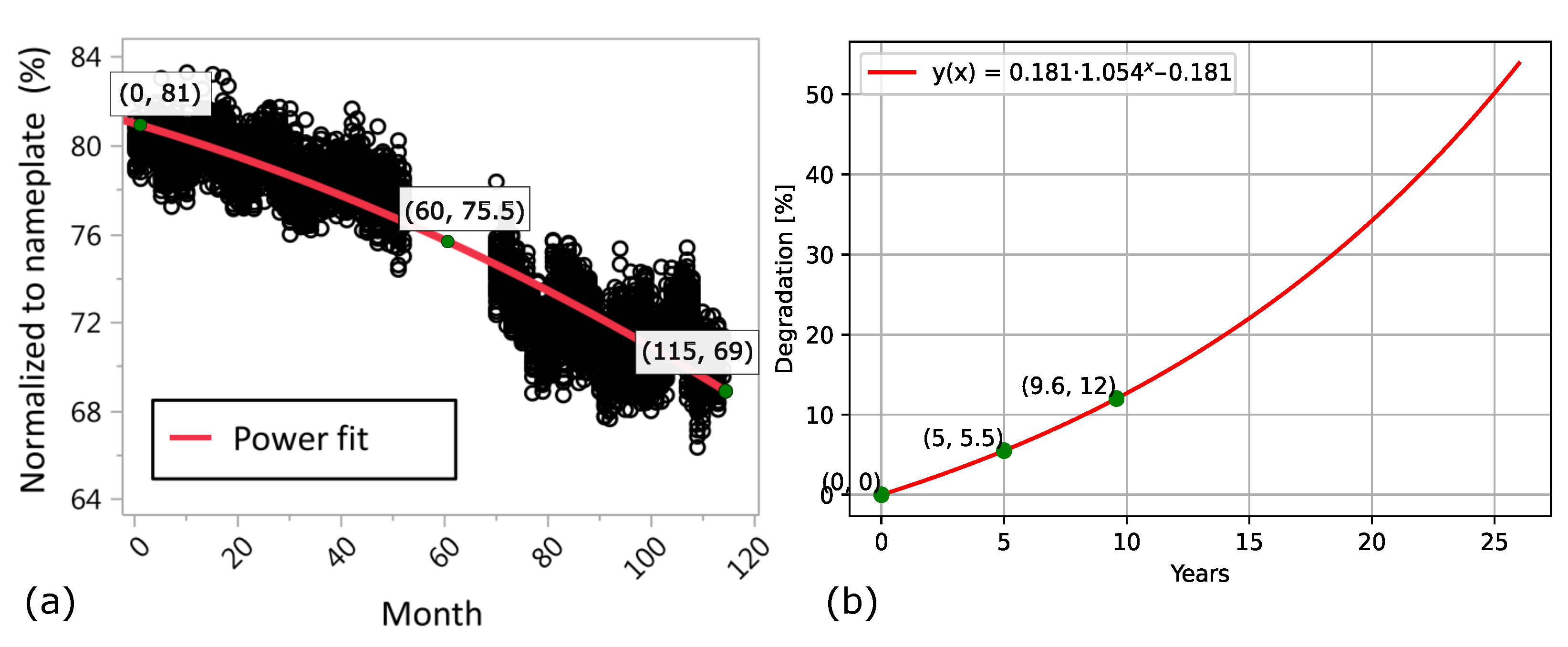
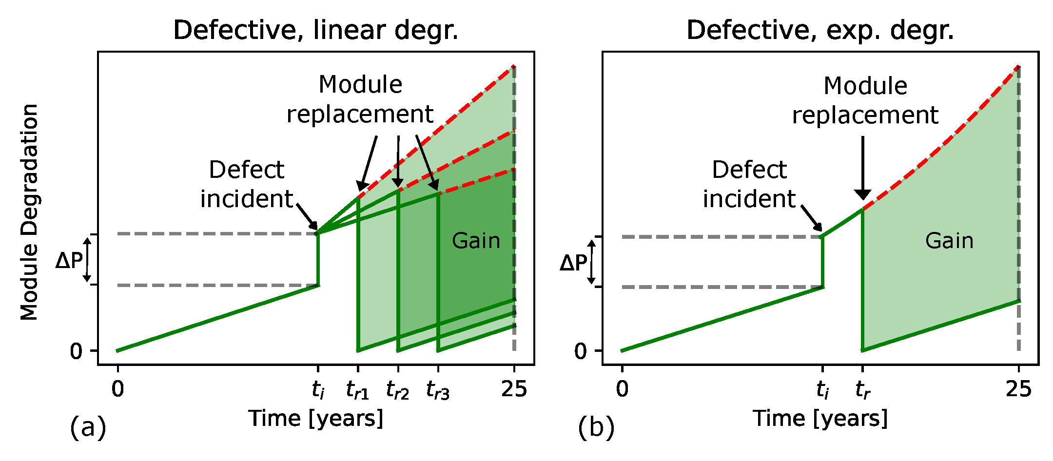
4.3. Cumulative Energy Loss from Defects and Degradation

The defect heating Δ T is often assumed proportional with the irradiance G [25,26], which Figure 4b supports as a fair assumption, where the Δ T of a bypassed substring is plotted against irradiation, showing a linear correlation. The relation between standard test conditions STC and inspection conditions i n s p . is therefore described as Δ T insp . / Δ T STC = G insp . / G STC . Combined with Equation (1), it follows that the defect power loss Δ P defect at the irradiance G insp . can be described as
Δ P defect = G insp . G STC · Δ P STC
If the relative amount of degradation is a linear rate d m per year, then the module degradation after t years at irradiance levels of G insp . can be expressed as
Δ P degr . , mod = G insp . G STC · P max · d m · t
where P max is the power production at STC of a defect-free module. The final contribution to degradation is the deterioration of defects, generally expressed to
Δ P degr . , defect = G insp . G STC · P max · y ( t )
where y(t) in this work will vary according to the defect degradation rates in Table 1. With these three contributions to the total power reduction, the cumulative energy loss after τ years can be found with
E loss = 0 τ Δ P tot dt = G insp . G STC ¯ · 0 τ Δ P STC + P max d m · t + y ( t ) dt
where G insp . G STC ¯ is the average irradiation over time τ .

4.4. Energy Gain from Module Replacement

With the cumulative module energy loss from Equation (6), the energy gain from module replacement at time tr can be calculated by comparing a scenario in which the defective module remains in place with one where it is replaced, and integrating the difference with respect to replacement time tr through a nominal 25-year lifetime:
E gain = t r 25 Δ P tot ( t ) Δ P degr . ,   mod ( t t r ) dt
which, for the linear defect degradation rates of dd, is written out as
E gain , lin . = G insp . G STC ¯ · t r 25 Δ P STC + P max d m + d d · t P max d m t t r dt
and for the exponential defect degradation rate is written out as
E gain , exp . = G insp . G STC ¯ · t r 25 Δ P STC + P max 0.181 · ( 1 . 055 t 1 ) P max d m t t r dt

5. Experimental Foundation

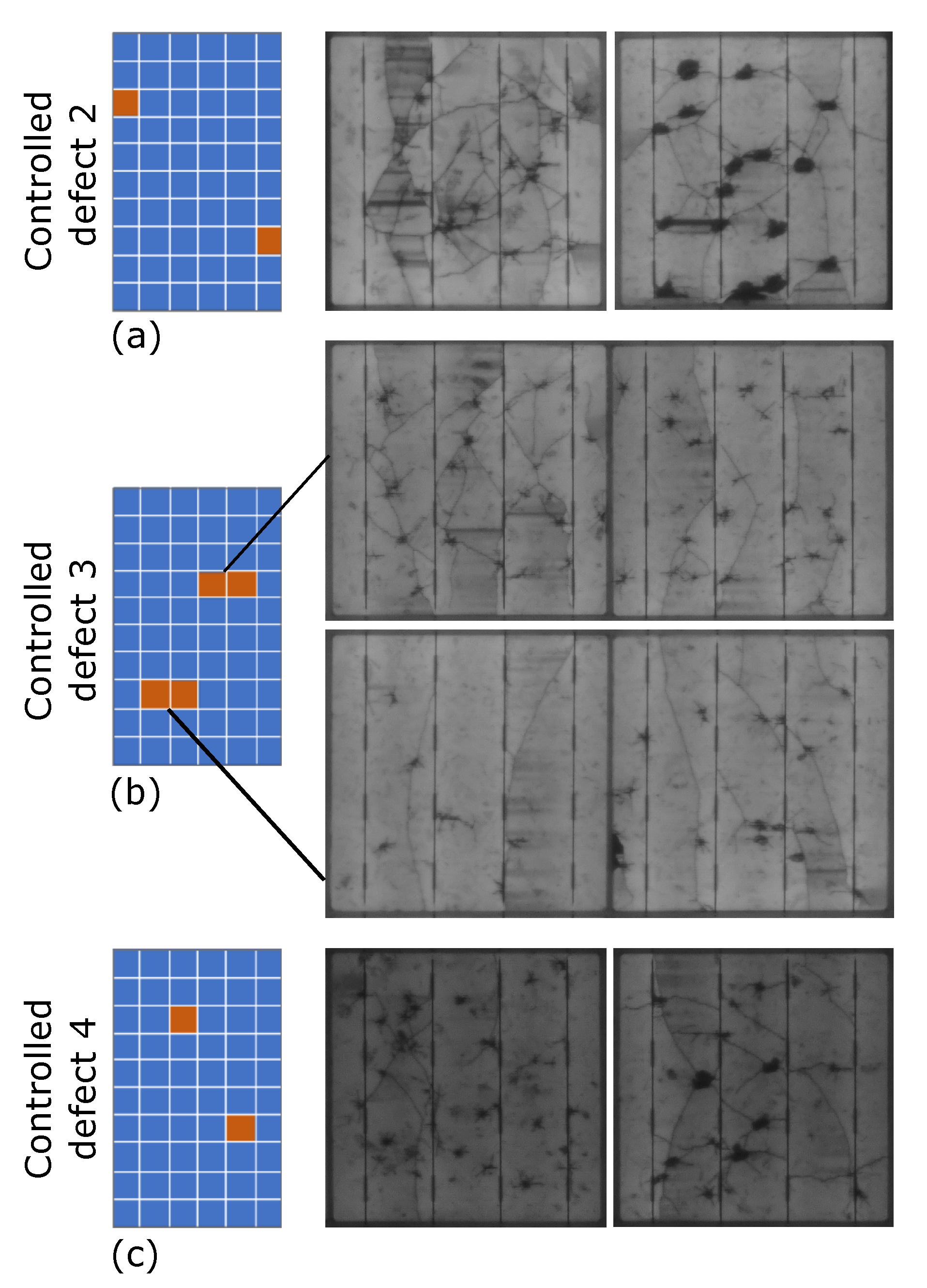
5.1. Characterization of Defects with Light IV and EL

The controlled defects were characterized with light IV measurements and EL imaging before and after damage was induced in 2020 to determine the impact of the defects. The EL images of the damaged cells are shown in Figure 5 for the following: (a) Controlled defect 2; (b) Controlled defect 3; (c) Controlled defect 4. The images reveal the presence of dark spots and lines, indicating inactive cell areas and cracks in all three modules at locations consistent with the sustained impact. The change in the module maximum power P max was measured with light IV measurements under standard test conditions: Table 2 shows P max for Controlled defect 1–4, measured before and after damage was inflicted (“Initial P max ” and “ P max post damage”) in 2020. Controlled defect 3, with its four impacted cells, exhibited the largest drop of −1.6%, while Controlled defect 2 has a measured positive change of 0.7% despite the damage seen from EL. The increase is within the measurement uncertainty of 0.3%, and it most likely does not represent an actual improvement in the module’s performance. The bypassed substring in Controlled defect 1 caused a power reduction of 35%, close to the expected 33% drop.

5.2. Power Loss from Park Defects

While the lab-induced defects are associated with a known power loss, the loss from the park defects is unknown. The power loss can, however, be assessed from the thermal images by using the bypassed substring in Controlled defect 1 as a reference for the relation between defect heating and power loss. With a known power loss of Δ P d 1 , and the corresponding Δ T d 1 available from the thermal images, we can find the proportionality constant between Δ P d 1 and Δ T d 1 , denoted k in Equation (2). This can, in turn, be used to approximate Δ P for the other modules based on their measured Δ T. We know that the power loss Δ P d 1 due to the substring failure is 95 W (see Table 2) when exposed to standard test conditions of 1000 W/m2. From the thermal images captured at the same irradiance, we can calculate the heating of the bypassed substring compared to the two functioning substrings at the same module as a measure of Δ T d 1 . Moreover, 1131 images were captured at an irradiance of 1000 ± 20 W/m2 during steady-state conditions, thus yielding
Δ T d 1 = 3.1 ± 1.2 K
where 3.1 K is the average value and 1.2 K is the standard deviation. With a defect area of 20 cells, it follows from Equation (2) that
k = Δ T d 1 · A Δ P d 1 = 3.1 K · 20 cells 95 W = 0.65 K · cells W
which gives the proportionality constant between Δ T and Δ P at 1000 W/m2. With all modules exposed to the same conditions, we can apply k to the Δ P calculations of the remaining modules, keeping in mind that different module models make this an approximation. The Δ T value of the park defects is obtained from the thermal images: 14,754 thermal images were taken during clear-sky conditions (the clear-sky filtering process is described in Section 4.1). As there are no reference modules of the same model as Controlled defect 1, Δ T is calculated by finding the mean temperature of the substring containing the hotspot (denoted “T2” in Figure 4a) and subtracting the mean temperature of the remaining two substrings in the module (denoted “T1” and “T3”). The obtained Δ Tsubs. is plotted against irradiation in Figure 4. At 1000 W/m2, we obtain Δ Tsubs. = 0.76 K. This can be used to calculate the corresponding energy loss at 1000 W/m2, using Equation (2), where A = 18 cells because we exclude the two cells in the substring affected by the heated bypassed diode (as shown in Figure 4a):
Δ P = Δ T · A k = 0.76 K · 18 cells 0.65 K · cells · W 1 = 21 W
This fits well with the characterizations of the module: The module was originally rated with a peak power of Pmax = 245 W in 2012 and 211 W in 2023. This reduction in performance of 34 W is likely caused by a combination of the defect, calculated to 21 W, and degradation. The yearly degradation rate can not be determined due to an unknown combination of storage and use since 2012.
As for Park defect 2, the heating of the hot spot is insufficient to be distinguished from noise.

6. Calculations on the Economic Impact of Defects

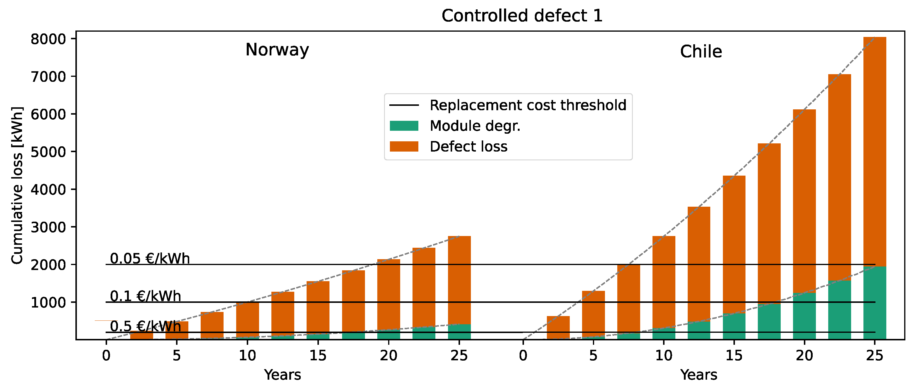
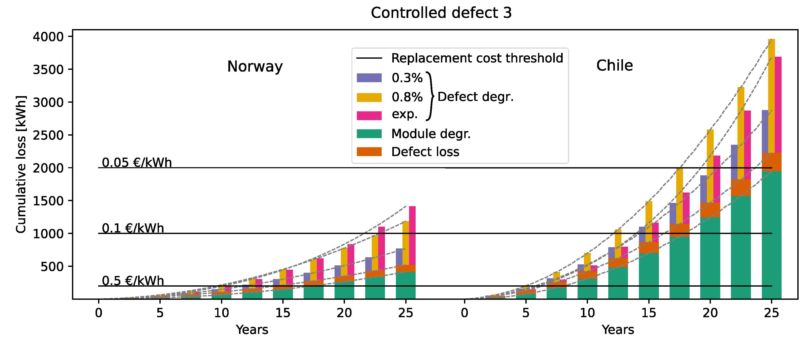
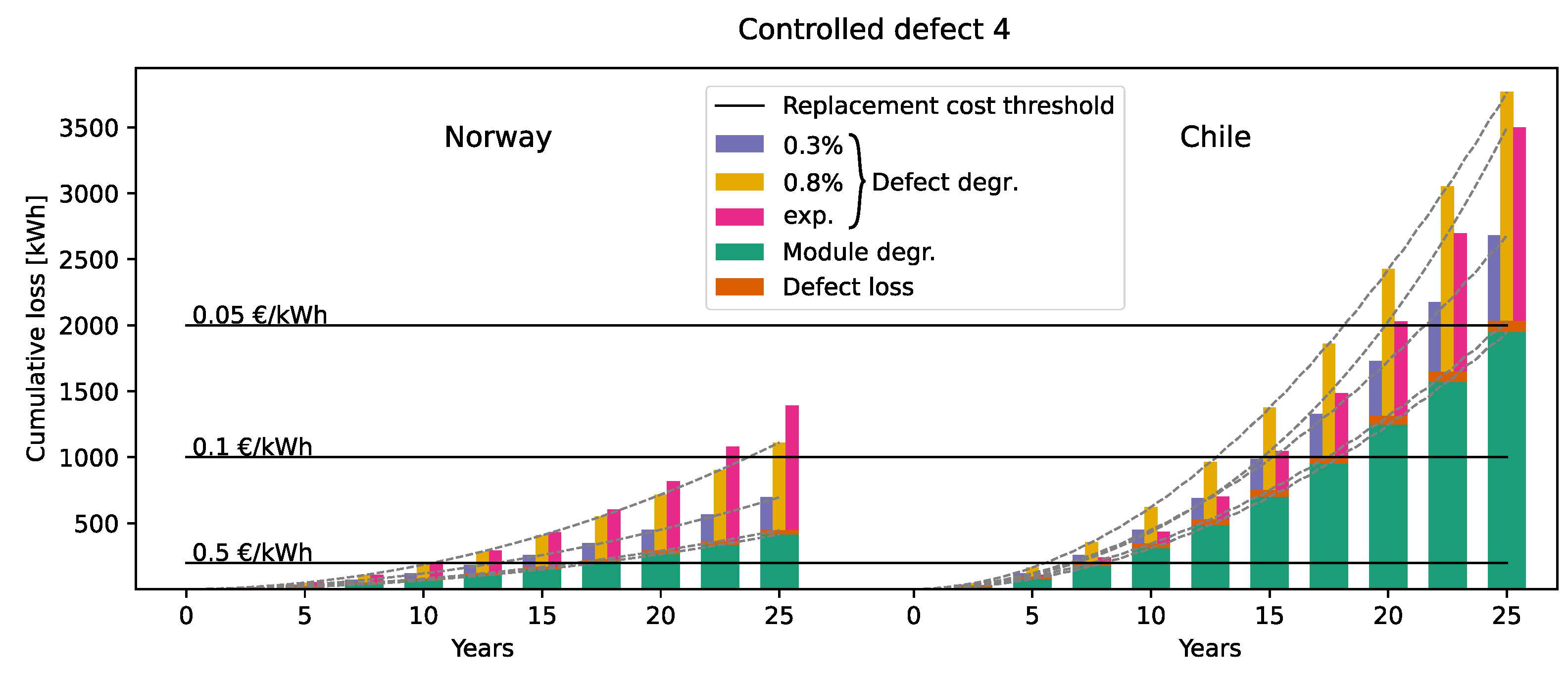
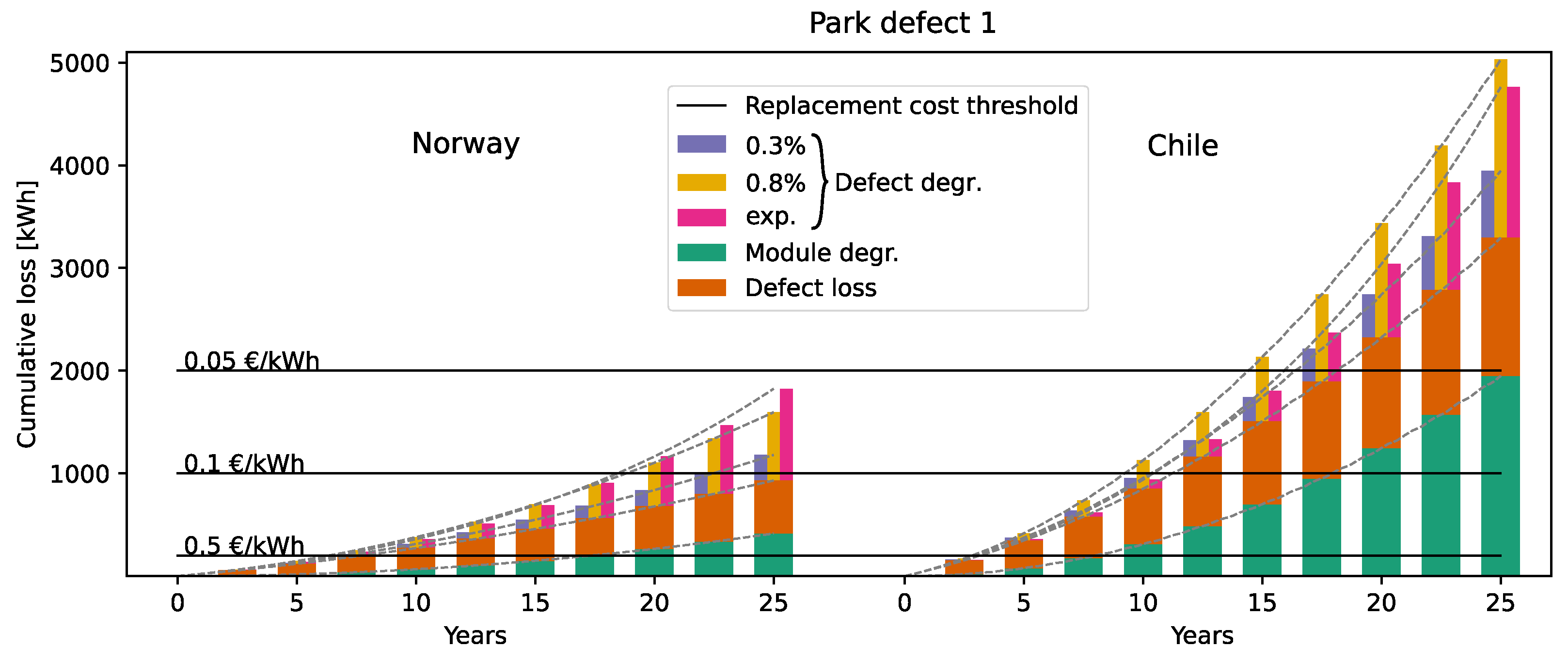
6.1. Cumulative Power Loss

With the module and defect degradation rates from Section 2, and defect losses from Section 5.1 and Section 5.2, the cumulative power loss is estimated with the calculations from Section 4.3, both for Norwegian and Chilean conditions. The required irradiance data were gathered from the module test site in Norway and from [27] for Chile. The calculations will assume a park lifetime of 25 years, complying with standard warranty periods, and assume that the defects are present from time t = 0. The P max values are found as “Initial P max ” in Table 2 (here assuming that the values represent new modules) for the controlled defects, and the measured P max = 211 W for Park defect 1.
To contextualize the energy loss, we compare it to the amount of energy a PV park operator must produce to offset the costs associated with module replacement. Both the cost of module replacement and the feed-in tariff price per kWh will vary with location and park size. The wholesale cost rate of a PV module is reported to be around EUR 0.22/W [28], constituting around EUR 60 for the 270 W modules in this study. We therefore assume a module replacement cost of EUR 100/module, which also includes the installation and other related costs. For simplicity, in the calculation of income losses, we assume that the income from PV power production is based on a fixed feed-in tariff. We investigate three different prices: EUR 0.05/kWh, EUR 0.1/kWh, and EUR 0.5/kWh [29]. With these assumptions, the cost of module replacement is covered by the production of 2000 kWh, 1000 kWh, and 200 kWh, respectively. This is plotted together with the energy loss as “Replacement cost threshold”. The actual value of park inspection with UAV-based thermography and subsequent module replacement depends on multiple factors, including local O&M costs and current and forecasted power prices, as well as costs of replacement modules [30]. Here, we focus on developing a generic methodology supporting fault detection and diagnostics (FDD) and subsequent prioritizing of O&M actions.
Figure 6 shows the cumulative energy loss from the bypassed substring in Controlled defect 1. We assume that the diode is not degrading, so no additional defect degradation is added to the power loss. The figure shows that the defect loss dominates over the module degradation loss. Figure 7, Figure 8 and Figure 9 show the cumulative energy loss from Controlled defect 3, 4, and Field defect 1, respectively. The four different defect degradation rates are shown side-by-side in the bar plot for comparison, where the fourth rate is a defect degradation of 0%. The figures demonstrate that degradation loss is the dominant factor for these smaller defects. Overall, the cumulative loss in Chile is more than double that in Norway, driven by both higher power production and a greater module degradation rate. Under Chilean conditions, the energy loss from all four modules exceeds the yield needed to cover the cost of module replacement at all three feed-in tariff levels. While the figures indicate that the energy loss from defective modules may surpass the energy required to offset replacement costs, they do not reveal the optimal timing for replacement. If a module is replaced at t = 0, it will still degrade along the curve shown by the green bars, whereas replacing the module at t = 12.5 years will reset the degradation. The optimal timing for module replacement will be examined in the next section.

6.2. Module Replacement Gain

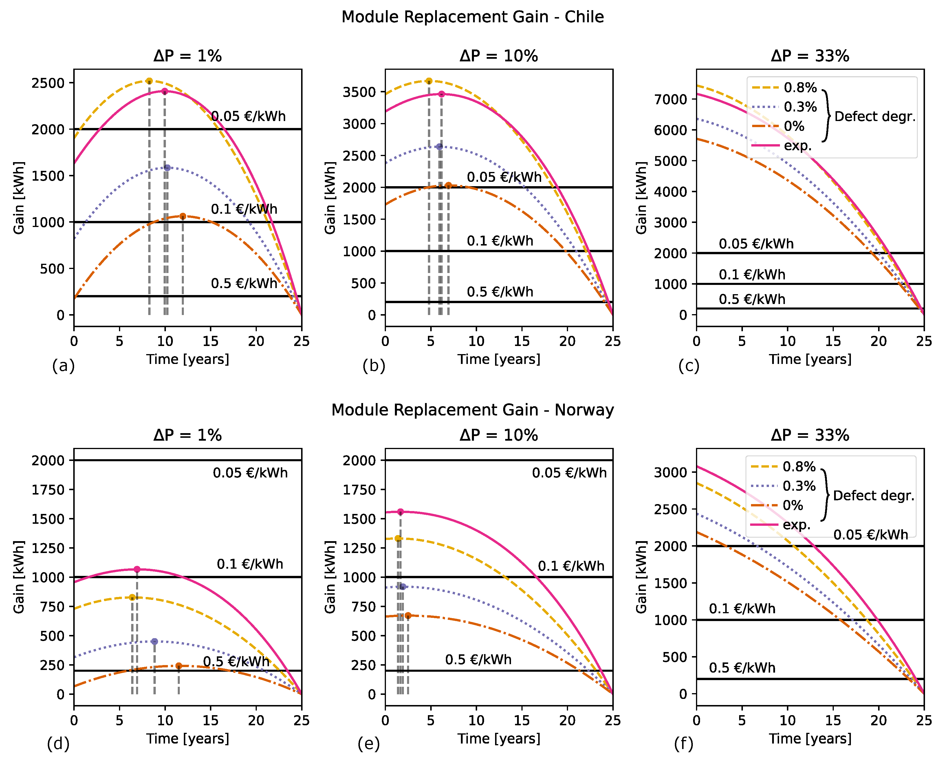
6.2.1. Infant-Life Failures

We will here calculate the energy gain from replacing defective modules at various points throughout the park’s 25-year lifespan. This is illustrated in Figure 10 for different scenarios: (a) Shows a non-defective module that degrades with time, where module replacement at time tr results in the energy gain shown in the green area. In (b), the defect Δ P degrades with three different linear degradation rates until module replacement at time tr, after which they degrade with the module degradation rate. (c) Shows the exponential degradation of a defect Δ P and the gain from replacing it at time tr. The gain can be calculated for varying tr by solving the integral of the degrading defective module minus the degrading non-defective module from time tr and to the end of the park life, as described in Section 4.4.
The gain will be compared with the same break-even thresholds as in previous section to determine if the energy gain from module replacement is higher than the cost of replacement, and therefore a cost-effective measure. The calculations assume that the defects are present from the beginning of the park’s lifetime, imitating infant-life failure defects arising from, e.g., manufacturing, transportation, or installation. The same degradation rates as in the previous section will be used, presented in Table 1, and three different defect losses of 1%, 10%, and 33% of the initial module Pmax. The 1% defect represents the inflicted cell damage in Controlled defects 3 and 4, the 10% defect is of the same severity as the Park defect 1, and the 33% defect represents the bypassed substring in Controlled defect 1. These three defect loss rates exemplify a minor module defect, a medium defect, and a severe defect.
The resulting energy gain is shown in Figure 11 for defects of Δ P = 1% in (a) (Chilean conditions) and (d) (Norwegian conditions), Δ P = 10% in (b) (Chilean conditions) and (e) (Norwegian conditions), and Δ P = 33% in (c) (Chilean conditions) and (f) (Norwegian conditions). The peak of the curves, representing the maximum gain, is marked with a dot. The cost of replacing the modules, converted to kWh, is shown as black lines for feed-in tariff prices of EUR 0.05/kWh, EUR 0.1/kWh, and EUR 0.5/kWh.
The general trends from the figures tell us that the following holds:
  • The most cost-effective approach is not necessarily to replace a defective module immediately; for the less severe defects, the peak occurs after some years of degradation.
  • The more significant the defects, the earlier the modules need to be replaced to ensure cost-effectiveness.
  • The minor defect of Δ P = 1% is most probably not cost-effective to replace in Norway unless the feed-in tariff prices are as high as EUR 0.5/kWh. For Chile, it can be beneficial to replace the module, but mainly if the module has sustained around 10 years of additional module degradation before it is replaced with a new module.
  • The medium-size defect with a loss of Δ P = 10% is cost-effective to replace in Chile, especially after around five years of additional module degradation, but it might not be cost-effective to replace in Norway.
  • The bypassed substring with a defect loss of Δ P = 33% is cost-effective to replace in both Norway and Chile, even if they are discovered late in the park life. This conclusion also extends to defects resulting in power losses greater than 33%.

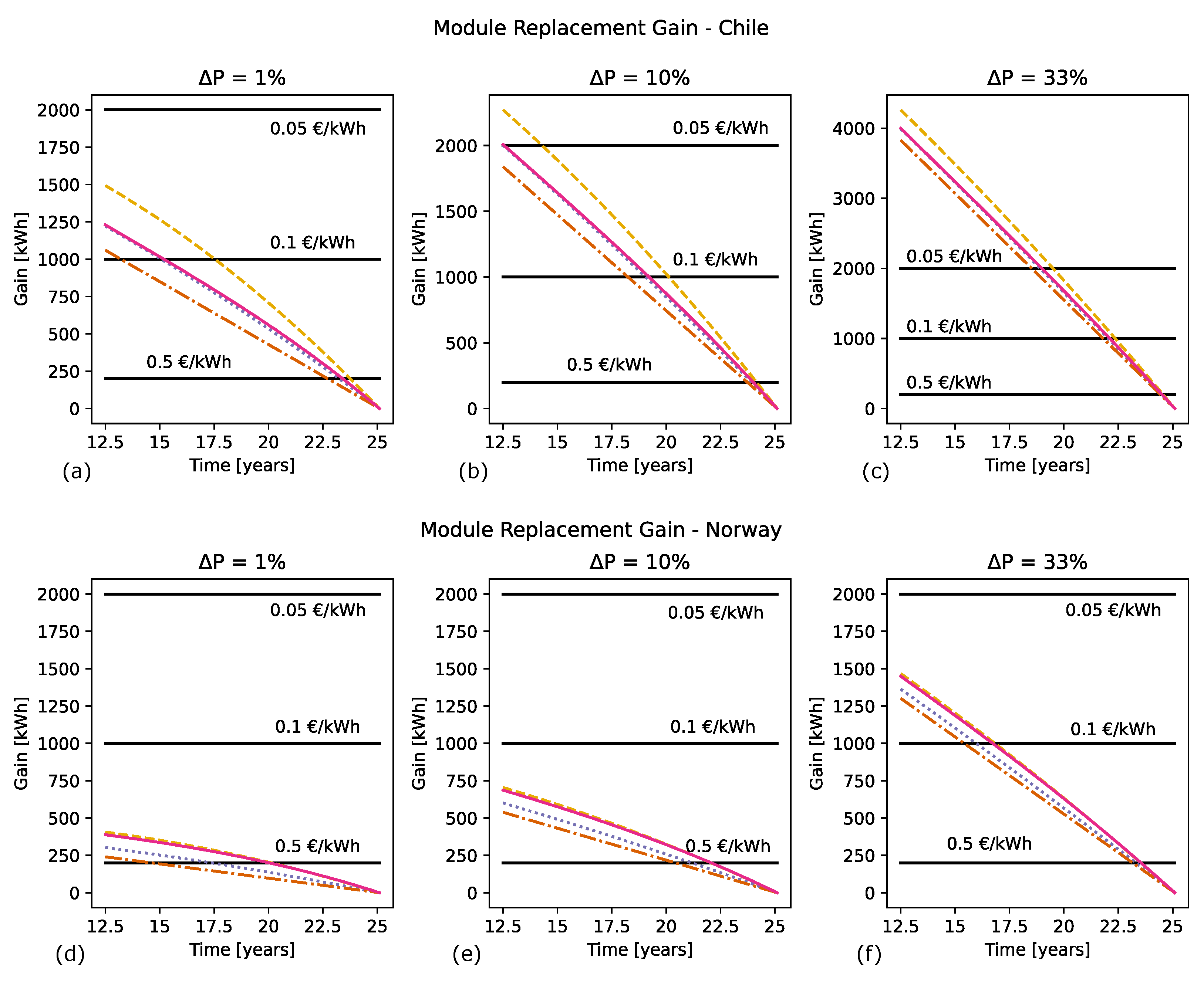
6.2.2. Mid-Life Failures

The cost-effectiveness of replacing defective modules will depend on when the defects occur. This section will evaluate whether it is beneficial to replace modules with defects that appear mid-life. Figure 12 illustrates a scenario where a defect with power loss Δ P occurs at time ti. The module degrades gradually until the defect incident, where Figure 12a shows the subsequent defect degradation as three different linear rates, and (b) illustrates the exponential defect degradation rate. The green areas demonstrate the gain from replacing the modules at time tr. This alters the module replacement gain, where Figure 13 shows a scenario where the defects occur halfway in the park life, at ti = 12.5 years. Figure 13a–c show a defect of 1%, 10%, and 33%, respectively, in Chilean conditions. Figure 13d–f show the same defects at Norwegian conditions. The key findings from the figure are as follows:
  • Unlike the infant-life failures in Figure 13, mid-life failures are most cost-effective to replace immediately.
  • Minor defects of 1% are most likely not cost-effective to replace, even in high-irradiation locations like Chile.
  • Defects of 10% are likely beneficial to replace mid-life in high-irradiation conditions, but not in low-irradiation locations like Norway.
  • For the more severe defect of 33%, there is a substantial gain from replacing the module in high-irradiation locations, even when they are not immediately detected. There might be a gain from replacing the 33% defects in low-irradiation conditions as well, given an early detection.
One additional aspect of mid-life O&M is that a module replacing a defective one after more than 10 years of operation will likely have a higher capacity due to technological advancements and a lower cost from increasing manufacturing. This gives an additional gain that would support the case for mid-life module replacement.

7. Summary and Conclusions

For this study, we established a test site with defective modules at Kjeller, Norway, as a foundation for assessments on the cost-effectiveness of module replacement. We demonstrated how the power loss from field-retrieved defects can be estimated based on thermal imagery, using a known defect as a reference. With the measured and estimated defect power losses, the long-term impact on power production is calculated both for low-irradiation locations like Norway and for high-irradiation countries like Chile. The first scenario assumed that the module defects were present from early park life. The cumulative power loss from the defect, defect degradation, and module degradation was used to calculate the energy gain from replacing the module at different times during a 25-year park lifetime. To assess whether replacing the module is cost-effective, the energy gain from module replacement is compared with the replacement cost and the energy selling price.
The main findings are that, for defects present from early-life, even minor defects, they are cost-effective to replace in high-irradiation locations. The timing is, however, crucial: The most significant benefits are achieved when modules with minor defects are replaced after approximately half of the park’s lifespan as the degradation at this point is considerable. This leads to a substantial increase in yield when it is replaced with a new module. For more severe defects, an earlier replacement is more favorable. For low-irradiation locations, the cost-effectiveness of replacing defective modules is uncertain unless the defect is as severe as a bypassed substring with its associated loss of 33%.
In the second scenario, the defects occurred mid-life after 12.5 years. In this case, the minor defects of 1% have an uncertain cost-effectiveness associated with module replacement at high-irradiation locations, while for medium defects of 10% and severe defects of 33%, the gain is likely substantial. In low-irradiation locations, the substring defect is most likely the only cost-effective module to replace out of the three example defects.
By comparing the consequences of module defects in high-irradiation and low-irradiation areas, our results suggest that O&M actions need to be adjusted based on the location. The cost of replacing modules is typically recouped more quickly in high-irradiation regions due to the higher energy yield, while more restrictive O&M actions can be beneficial in low-irradiation areas like Norway. While most PV park O&M activities include both performance monitoring systems and module inspections, small or remote PV parks may choose to minimize O&M activities to reduce costs, especially when access to skilled labor is difficult. Simplifying O&M practices can be more justifiable in low-irradiation regions where the energy losses due to unmaintained defects are less pronounced.

Author Contributions

Conceptualization, V.L.-L.; data curation, B.L.A. and N.R.; formal analysis, V.L.-L.; methodology, V.L.-L. and B.L.A.; supervision, B.L.A., E.S.M. and T.S.; visualization, V.L.-L.; writing—original draft, V.L.-L. All authors have read and agreed to the published version of the manuscript.

Funding

This research received no external funding.

Data Availability Statement

The raw data supporting the conclusions of this article will be made available by the authors on request.

Conflicts of Interest

The authors declare no conflicts of interest.

Appendix A

In order to find the function that describes the defect degradation rate in Figure A1a from [19], the authors extracted three coordinates, which are marked in the figure, and performed a curve fitting. The fitted curve, shown as module degradation as opposite the module gain, is shown in Figure A1 with the associated function. It can be noted that reading out the coordinates from the graph might lead to slight inaccuracies, which will affect the obtained function.
Figure A1. (a) Figure from [19] (coordinates added by author) of the yield of a defective module. (b) Defect degradation based on curve fitting of coordinates from (a).
Solar 04 00034 g0a1

References

  1. Li, L.; Lin, J.; Wu, N.; Xie, S.; Meng, C.; Zheng, Y.; Wang, X.; Zhao, Y. Review and outlook on the international renewable energy development. Energy Built Environ. 2022, 3, 139–157. [Google Scholar] [CrossRef]
  2. International Renewable Energy Agency. Renewable Power Generation Costs in 2022; Technical Report; International Renewable Energy Agency (IRENA): Abu Dhabi, United Arab Emirates, 2023. [Google Scholar]
  3. Mahdi, A.; Leahy, H.; Alghoul, P.G.; Morrison, M.; Al Mahdi, H.; Leahy, P.G.; Alghoul, M.; Morrison, A.P. A Review of Photovoltaic Module Failure and Degradation Mechanisms: Causes and Detection Techniques. Solar 2024, 4, 43–82. [Google Scholar] [CrossRef]
  4. Rajput, P.; Singh, D.; Singh, K.Y.; Karthick, A.; Shah, M.A.; Meena, R.S.; Zahra, M.M.A. A comprehensive review on reliability and degradation of PV modules based on failure modes and effect analysis. Int. J. Low-Carbon Technol. 2024, 19, 922–937. [Google Scholar] [CrossRef]
  5. International Energy Agency (IEA). Review of Failures of Photovoltaic Modules; Technical Report; International Energy Agency (IEA): Paris, France, 2014. [Google Scholar]
  6. Buerhop, C.; Bommes, L.; Schlipf, J.; Pickel, T.; Fladung, A.; Peters, I.M. Infrared imaging of photovoltaic modules: A review of the state of the art and future challenges facing gigawatt photovoltaic power stations. Prog. Energy 2022, 4, 042010. [Google Scholar] [CrossRef]
  7. Kirsten Vidal de Oliveira, A.; Aghaei, M.; Rüther, R. Aerial infrared thermography for low-cost and fast fault detection in utility-scale PV power plants. Sol. Energy 2020, 211, 712–724. [Google Scholar] [CrossRef]
  8. Herz, M.; Friesen, G.; Jahn, U.; Koentges, M.; Lindig, S.; Moser, D. Identify, analyse and mitigate—Quantification of technical risks in PV power systems. Prog. Photovoltaics Res. Appl. 2023, 31, 1285–1298. [Google Scholar] [CrossRef]
  9. Moser, D.; Del Buono, M.; Jahn, U.; Herz, M.; Richter, M.; De Brabandere, K. Identification of technical risks in the photovoltaic value chain and quantification of the economic impact. Prog. Photovoltaics Res. Appl. 2017, 25, 592–604. [Google Scholar] [CrossRef]
  10. International Energy Agency (IEA). Quantification of Technical Risks in PV Power Systems Task 13 Performance, Operation and Reliability of Photovoltaic Systems Identify Analyse Mitigate; International Energy Agency (IEA): Paris, France, 2021. [Google Scholar]
  11. Kim, J.; Rabelo, M.; Padi, S.P.; Yousuf, H.; Cho, E.C.; Yi, J. A review of the degradation of photovoltaic modules for life expectancy. Energies 2021, 14, 4278. [Google Scholar] [CrossRef]
  12. Aghaei, M.; Fairbrother, A.; Gok, A.; Ahmad, S.; Kazim, S.; Lobato, K.; Oreski, G.; Reinders, A.; Schmitz, J.; Theelen, M.; et al. Review of degradation and failure phenomena in photovoltaic modules. Renew. Sustain. Energy Rev. 2022, 159, 112160. [Google Scholar] [CrossRef]
  13. Jordan, D.C.; Wohlgemuth, J.H.; Kurtz, S.R. Technology and climate trends in pv module degradation. In Proceedings of the 27th European Photovoltaic Solar Energy Conference and Exhibition, Frankfurt, Germany, 24–28 September 2012; pp. 3118–3124. [Google Scholar] [CrossRef]
  14. Dubey, R.; Chattopadhyay, S.; Kuthanazhi, V.; Kottantharayil, A.; Singh Solanki, C.; Arora, B.M.; Narasimhan, K.L.; Vasi, J.; Bora, B.; Singh, Y.K.; et al. Comprehensive study of performance degradation of field-mounted photovoltaic modules in India. Energy Sci. Eng. 2017, 5, 51–64. [Google Scholar] [CrossRef]
  15. Jordan, D.C.; Kurtz, S.R.; VanSant, K.; Newmiller, J. Compendium of photovoltaic degradation rates. Prog. Photovoltaics Res. Appl. 2016, 24, 978–989. [Google Scholar] [CrossRef]
  16. Singh, J.; Belmont, J.; TamizhMani, G. Degradation analysis of 1900 PV modules in a hot-dry climate: Results after 12 to 18 years of field exposure. In Proceedings of the 2013 IEEE 39th Photovoltaic Specialists Conference (PVSC), Tampa, FL, USA, 16–21 June 2013; pp. 3270–3275. [Google Scholar] [CrossRef]
  17. Deceglie, M.G.; Silverman, T.J.; Member, S.; Young, E.; Hobbs, W.B.; Member, S.; Libby, C. Field and Accelerated Aging of Cracked Solar Cells. IEEE J. Photovoltaics 2023, 13, 836–841. [Google Scholar] [CrossRef]
  18. Suleske, A.; Singh, J.; Kuitche, J.; Tamizh-Mani, G. Performance degradation of grid-tied photovoltaic modules in a hot-dry climatic condition. In Proceedings of the Reliability of Photovoltaic Cells, Modules, Components, and Systems IV, San Diego, CA, USA, 22–25 August 2011; Volume 8112, p. 81120P. [Google Scholar] [CrossRef]
  19. Jordan, D.C.; Silverman, T.J.; Sekulic, B.; Kurtz, S.R. PV degradation curves: Non-linearities and failure modes. Prog. Photovoltaics Res. Appl. 2017, 25, 583–591. [Google Scholar] [CrossRef]
  20. Buerhop, C.; Wirsching, S.; Bemm, A.; Pickel, T.; Hohmann, P.; Nieß, M.; Vodermayer, C.; Huber, A.; Glück, B.; Mergheim, J.; et al. Evolution of cell cracks in PV-modules under field and laboratory conditions. Prog. Photovoltaics Res. Appl. 2018, 26, 261–272. [Google Scholar] [CrossRef]
  21. IEC 60904-9; Photovoltaic Devices—Part 9: Solar Simulator Performance Requirements. International Electrotechnical Commission: Geneva, Switzerland, 2007.
  22. IEC TS 60904-13; Photovoltaic Devices—Part 13: Electroluminescence of Photovoltaic Modules. International Electrotechnical Commission: Geneva, Switzerland, 2018.
  23. Holmgren, W.F.; Hansen, C.W.; Mikofski, M.A. pvlib python: A python package for modeling solar energy systems. J. Open Source Softw. 2018, 3, 884. [Google Scholar] [CrossRef]
  24. Teubner, J.; Buerhop, C.; Pickel, T.; Hauch, J.; Camus, C.; Brabec, C.J. Quantitative assessment of the power loss of silicon PV modules by IR thermography and its dependence on data-filtering criteria. Prog. Photovoltaics Res. Appl. 2019, 27, 856–868. [Google Scholar] [CrossRef]
  25. Moretón, R.; Lorenzo, E.; Narvarte, L. Experimental observations on hot-spots and derived acceptance/rejection criteria. Sol. Energy 2015, 118, 28–40. [Google Scholar] [CrossRef]
  26. Dhimish, M.; Badran, G. Investigating defects and annual degradation in UK solar PV installations through thermographic and electroluminescent surveys. npj Mater. Degrad. 2023, 7, 14. [Google Scholar] [CrossRef]
  27. National Solar Radiation Database. 2024. Available online: https://nsrdb.nrel.gov/data-viewer (accessed on 12 August 2024).
  28. Solar Module Prices Increase for First Time in Years, Anza Reports—pv Magazine USA. 2014. Available online: https://pv-magazine-usa.com/2024/06/12/solar-module-prices-increase-for-first-time-in-years-anza-reports/ (accessed on 26 September 2024).
  29. Feed-in Tariffs (FITs) in Europe—pv Magazine International. 2024. Available online: https://www.pv-magazine.com/features/archive/solar-incentives-and-fits/feed-in-tariffs-in-europe/ (accessed on 26 September 2024).
  30. Aarseth, B.L.; Nygård, M.M.; Otnes, G.; Marstein, E.S. Combining Production Data Timeseries and Infrared Thermography to Assess the Impact of Thermal Signatures on Photovoltaic Yield Over Time. IEEE J. Photovoltaics 2024. early access. [Google Scholar] [CrossRef]
Figure 1. The average module degradation rate is plotted in green for the following: (a) Norway; (b) Chile. Additionally, four different defect degradation rates are added to the general module degradation. The exponential defect degradation is not separated from the module degradation, and is therefore the same for both locations.
Solar 04 00034 g001
Figure 2. Thermal image of the module test site. The “Controlled defects” are deliberately created and consist of a bypassed substring (Controlled defect 1) and cell cracks (Controlled defects 2 to 4). The “Park defects” are collected from a solar park and have cell hotspots. Refs. 1 and 2 are reference modules. The image is taken at a solar irradiance of 600 W/m2 in the module plane.
Solar 04 00034 g002
Figure 3. The measured Global Horizontal Irradiance (GHI) at the test site is shown in red, and the modeled GHI in purple. Clear-sky conditions are highlighted in green, and clear-sky conditions that have not yet reached steady-state are depicted in yellow, labeled as ‘Unstable clear-sky’.
Solar 04 00034 g003
Figure 4. (a) Park defect 1. The mean temperature of each substring is used to calculate Δ Tsubs., here defined as the temperature difference between the substring with a hotspot minus the mean temperature of the remaining two substrings. The calculations are shown above the module. (b) The obtained Δ Tsubs. values for Park defect 1 are plotted against the irradiance. The running median and linear regression with R2 = 0.53 are shown.
Solar 04 00034 g004
Figure 5. Electroluminescence images of the inflicted cell damage in the following: (a) Controlled defect 2; (b) Controlled defect 3; (c) Controlled defect 4. The orange cells in the left panels show the location of the damaged cells in the module.
Solar 04 00034 g005
Figure 6. Cumulative power loss from Controlled defect 1 (bypassed substring) for conditions representative of Norway (left) and Chile (right). The power loss is decomposed into module degradation (green) and defect loss (red), with dotted lines showing the trend for each component.
Solar 04 00034 g006
Figure 7. Cumulative power loss from Controlled defect 3 (cell cracks) for conditions representative of Norway (left) and Chile (right). The power loss is decomposed into module degradation (green), defect loss (red), and three different defect degradation rates presented in Table 1. The dotted lines show the trend for each component.
Solar 04 00034 g007
Figure 8. Cumulative power loss from Controlled defect 4 (cell cracks) for conditions representative of Norway (left) and Chile (right). The power loss is decomposed into module degradation (green), defect loss (red), and three different defect degradation rates presented in Table 1. The dotted lines show the trend for each component.
Solar 04 00034 g008
Figure 9. Cumulative power loss from Park defect 1 (hotspot) for conditions representative of Norway (left) and Chile (right). The power loss is decomposed into module degradation (green), defect loss (red), and three different defect degradation rates presented in Table 1. The dotted lines show the trend for each component.
Solar 04 00034 g009
Figure 10. Illustration of the module degradation for the following: (a) A non-defective module; (b) A defect with a loss of Δ P and three different linear defect degradation rates; (c) A defect Δ P with an exponential degradation. The green areas illustrate the gain from module replacement at time tr, and the red, dashed lines show the scenario where the modules are not replaced.
Solar 04 00034 g010
Figure 11. Module replacement gain for different defects Δ P and degradation rates. Conditions representative of Chile are shown in (ac) and of Norway in (df). The horizontal lines show the cost of module replacement converted to kWh for three different feed-in tariffs of EUR 0.05/kWh, EUR 0.1/kWh, and EUR 0.5/kWh.
Solar 04 00034 g011
Figure 12. Illustration of a defect Δ P occurring at time ti: (a) Three different linear defect degradation rates are shown; (b) An exponential defect degradation rate. The green areas illustrate the gain from module replacement at time tr, and the red, dashed lines show the scenario where the modules are not replaced.
Solar 04 00034 g012
Figure 13. Module replacement gain for different defects Δ P occurring mid-life, after 12.5 years. The gain is shown for different defect degradation rates. Conditions representative for Chile are shown in (ac), and Norwegian conditions in (df). The horizontal lines show the cost of module replacement converted to kWh for three different feed-in tariffs of EUR 0.05/kWh, EUR 0.1/kWh, and EUR 0.5/kWh.
Solar 04 00034 g013
Table 1. Reported module degradation rates typical for the climates in Chile and Norway, and different defect degradation rates found in literature.
Type of Degradation Degradation Rate per Year
Module degradationChile0.9%
Norway0.5%
Defect degradation[20]0%
[17]0.3%
[18]0.8%
[19]Increasing: 0.181 · (1.055t − 1) where t is time in years
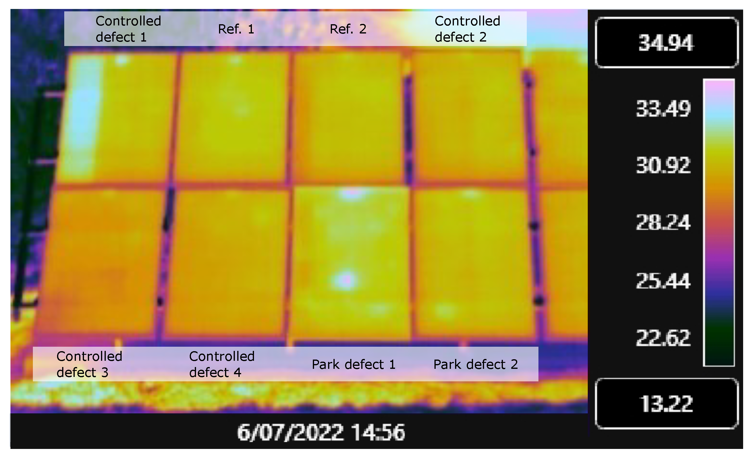
Table 2. Maximum power from light IV measurements at standard test conditions before and after inflicted module damage.
ModuleInitial P max [W] P max Post Damage [W]ΔP [W]Relative Change
Contr. defect 1270.5175.8−95−35%
Contr. defect 2270.4272.21.80.7%
Contr. defect 3274.4270.1−4.3−1.6%
Contr. defect 4269.5268.2−1.3−0.5%
Disclaimer/Publisher’s Note: The statements, opinions and data contained in all publications are solely those of the individual author(s) and contributor(s) and not of MDPI and/or the editor(s). MDPI and/or the editor(s) disclaim responsibility for any injury to people or property resulting from any ideas, methods, instructions or products referred to in the content.

