Article

Optimal Strategies for Interval Economic Order Quantity (IEOQ) Model with Hybrid Price-Dependent Demand via C-U Optimization Technique

by
Md Sadikur Rahman
Department of Mathematics, Khalisani Mahavidyalaya, Khalisani, Hooghly, Chandannagar 712138, West Bengal, India
AppliedMath 2025, 5(4), 151; https://doi.org/10.3390/appliedmath5040151
Submission received: 12 September 2025 / Revised: 28 October 2025 / Accepted: 28 October 2025 / Published: 5 November 2025

Abstract

In inventory management, business organizations gradually face challenges due to the complexities of managing perishable goods whose value diminishes over time. In such circumstances, interval’s bounds estimated business policy can be adopted to study a non-deterministic inventory model incorporating decay, preservation technology, and financial incentives, viz. advanced payments and fixed discounts. This study explores an interval Economic Order Quantity (EOQ) model incorporating advanced payment with discount options under preservation technology framework in interval environment. In this model, the demand rate is expressed as a convex combination of linear and power patterns of the selling price. The present model is formulated mathematically using interval differential equations and interval mathematics. Then, the corresponding interval-valued average profit of the model is obtained. In order to optimize the corresponding interval optimization problem, C-U optimization technique is developed. Employing the C-U optimization technique, the said interval optimization problem is converted into crisp optimization problems. Then, these problems are solved numerically by Wolfrom MATHEMATICA-11.0 software and validated with the help of two numerical examples. Finally, sensitivity analyses have been performed to study the impact of known inventory parameters on optimal policy.

1. Introduction

Inventory management is a vital branch in operations research for business operations as it balances the trade-offs between stockouts, overstocks, holding costs, and ordering costs. Stockout causes lost sales and customer dissatisfaction, while overstock increases holding and deterioration costs, and frequent ordering raises setup expenses. To evaluate these trade-offs, inventory valuation methods such as FIFO, LIFO, and weighted average are often applied in practice. From a theoretical perspective, various inventory models have been developed to capture such complexities in deterministic and non-deterministic models. Inventory models provide structured approaches to minimize costs and maximize profits under varying conditions. Depending on how uncertainty is treated, models can be broadly categorized into deterministic (crisp) inventory models, where all parameters are assumed to be precise; stochastic or probabilistic models, where parameters such as demand or lead time are random variables; fuzzy inventory models, which incorporate imprecise or vague information through fuzzy sets; and interval inventory models, where uncertain parameters are represented by intervals. Each modeling framework has been developed to address real-world issues such as demand fluctuation, deterioration of goods, shortages, advanced payment policies, and preservation technologies.
In a crisp inventory model, all important factors influencing the optimal policy, viz. customer demand, deterioration rate, preservation technology, per unit holding cost, and backlogging parameters are precise. The demand rate typically fluctuates based on factors viz., stock level, selling price, reliability, product freshness, and time. Although deterioration of commodities is unavoidable, it can be mitigated using preservation technology. Various studies have incorporated these realistic assumptions. Notable research on deteriorating items with preservation technology include works by Dye and Yang [1], Panda et al. [2], and Adak and Mahapatra [3]. Skouri and Papachristos [4], San-José et al. [5] studied few inventory models with variable demand under backlogging. Rahman et al. [6] solved an inventory problem with hybrid price and stock-dependent variable demand under preservation technology and backlogging. Xu et al. [7] looked into an inventory model for nonperishable items with trapezoidal demand. The per unit holding cost, another critical characteristic, is typically assumed to be constant but can occasionally vary over time or with order quantity. Further research on pricing inventory models with time-varying holding costs was conducted by Karmakar [8] and Yadav and Swami [9]. Advanced business policies, such as advanced payment, delayed payment, trade credit policy, and discount facilities add realism to various inventory models. These policies aim to reduce business risk by requiring customers to pay the total or a fraction of the purchase cost in advance. In this area, some notable contributions were made by Soto et al. [10], Taleizadeh [11], Shaikh et al. [12], and Khan et al. [13].
In a stochastic inventory model, the factors such as demand rate, deterioration rate, defective rate, and lead time are typically treated as random variables with specific probability distributions. Optimal policies are determined by calculating expected values of average profit, average cost, and other factors. In this area, some notable works were accomplished by Taleizadeh et al. [14] on probabilistic replenishment intervals, and Mondal et al. [15] on inventory models for ameliorating items with random amelioration and deterioration. In a fuzzy inventory model, some or all parameters are presented by fuzzy sets/numbers. In this area, notable contributions were accomplished by Rahaman et al. [16] on imprecise production inventory models with fuzzy differential equations, and Sadeghi et al. [17] on inventory models with fuzzy demand. Other significant works were performed by Ghorabaee et al. [18], Mondal [19], and Shaikh et al. [20]. In interval inventory model, imprecise parameters are presented in the form of intervals. In this area, Bhunia and Shaikh [21], Bhunia et al. [22], Kumar and Keerthika [23], Ruidas et al. [24], and Shaikh et al. [25] made their contributions under several assumptions. Rahman et al. [26,27,28] introduced interval-valued demand as well as deterioration rates in the formulation of their models and studied optimal policies using interval differential equations and parametric approaches.
Optimization techniques play a crucial role in studying the optimal policy of inventory control/supply chain problems. To study optimal policy, several researchers employed different techniques based on their model complexities. Cuevas et al. [29], Sajadi and Ahmadi [30], Huang [31], and many other researchers used different metaheuristic algorithms to find the optimal policies of their proposed inventory/supply chain problems. On the other hand, de Paula Vidal et al. [32] and Saha et al. [33] applied fuzzy optimization methods along with genetic algorithm differential evaluation and artificial neural networks for finding models’ optimal policy. In the case of the interval inventory control problem, Rahman et al. [27] first used the center–radius optimization technique along with different variants of QPSOs to study the optimal policy of their considered model. After that, Manna and Bhunia [34] used an improved center–radius technique along with various metaheuristics to investigate the optimal policy of a green production inventory problem. Recently, Duary et al. [35] studied the optimal policy of an interval production problem using 0–1 parametrized optimization technique. The present study proposes a new interval optimization technique based on the center and upper bound of an interval called the C-U optimization technique to study the optimality of the proposed interval inventory control problem.
To underscore the significant research gaps, a comparative analysis related to previous studies is presented in Table 1.
Despite the rich literature on crisp, stochastic, fuzzy, and interval inventory models, most of these studies contained only a limited number of real-world complexities. For instance, models with interval-valued demand rarely consider the combined effects of preservation technology, advanced payment schemes, and discount facilities. To be specific, in the literature of crisp inventory models, the hybrid effects of linear and power patterns of selling price have been considered, but no one accomplished this in the case of imprecise inventory models like fuzzy, interval, etc. On the other hand, while variable holding costs have been explored, the case where holding cost per unit changes linearly with stock level under interval uncertainty has not received much attention. Moreover, few works use interval differential equations as a formal tool to capture demand uncertainty and then optimize profit under such a setting, but no one has used the center and upper bound-based optimization technique to date. These gaps highlight the need for a more integrated framework that captures multiple practical factors simultaneously.
To address these gaps, this paper develops an interval Economic Order Quantity (EOQ) framework named as the IEOQ framework that captures nonlinear price-dependent demand, preservation technology, and financial factors such as advance payment and fixed discounts. The model is distinctive in incorporating advanced payment options and fixed discount facilities, while considering that holding costs per unit vary linearly with stock levels. To address the inherent uncertainties, the model uses interval differential equations and interval arithmetic for its mathematical formulation. The primary objective is to maximize the interval-valued average profit, which is achieved through the Center–Upper bound (C-U) optimization technique implemented in Wolfrom MATHEMATICA-11.0 software.
Although the EOQ framework is classical, it remains relevant because of its flexibility to accommodate modern extensions. EOQ offers a clear analytical base that can be modified for stochastic, fuzzy, or interval environments. In the case of a stochastic or fuzzy EOQ framework, the researchers have to make extra decisions regarding the selection of an appropriate probability distribution/fuzzy membership function during the representation of imprecise parameters. On the other hand, in the case of an IEOQ framework, the representation of imprecise parameters is simply made by the parametric form of interval. In contrast, the Economic Production Quantity (EPQ) model is production-oriented and less suited for the purchasing–inventory situations considered here. Therefore, the present work studies the optimal policy of an IEOQ model under uncertain, interval-driven business settings.
This study makes the following novel contributions:
  • It proposes an interval EOQ (IEOQ) framework in parametric form for perishable goods where demand rate is an interval-valued function which is the hybridization of linear and power pattern functions of selling price.
  • The model uniquely combines advanced payment, preservation technology, and fixed discount facilities with interval uncertainty, an aspect not jointly addressed in earlier research.
  • Unlike most existing works, the holding cost per unit is assumed to vary linearly with stock levels in an interval environment, capturing a more realistic cost structure.
  • The work employs interval differential equations, interval parametric mathematics to obtain the interval-valued average profit and solves it using interval order relation-based optimization technique.
  • The notable novel contribution of this work is the introduction of a new interval optimization technique named the C-U optimization technique to maximize interval-valued average profit.

2. Defining the Problem, Assumptions, and Notation

2.1. Problem Definition

The EOQ model is one of the most established frameworks in inventory theory because of its adaptability and analytical clarity. Although it is a traditional approach, its basic structure allows meaningful modification to incorporate uncertainty, financial policies, and sustainability aspects.
Under uncertainty, several researchers generalized the traditional EOQ models by tackling challenges of representing real-world parameters which are rarely precise. In recent years, numerous inventory models have been developed under interval and imprecise settings, addressing deterioration, price- and stock-dependent demand, payment policies, and sustainability [22,28,31,32,33,34,35]. These studies confirm that advanced mathematical approaches can provide optimal strategies for uncertain environments. However, very few works have jointly considered interval-valued demand, nonlinear price effects, preservation technology, and advance payment discounts within a unified EOQ framework. Building on this gap, our study extends the EOQ model into an interval environment while incorporating early payment discounts, loans, and preservation technology, thereby bridging the gap between theoretical extensions and practical relevance. In this study, we extend the EOQ framework to an interval environment named interval EOQ (IEOQ) framework, where key parameters are interval-valued, making it suitable for imprecise demand and cost conditions. The model further considers a realistic payment scenario in which vendors offer early payment discounts: buyers who pay in advance receive an interval-valued discount on the purchasing cost. Customers with insufficient cash may rely on bank loans at a fixed interest rate, while vendors use this discount scheme to retain buyers and remain competitive.
The formulation of the proposed model, including basic notations and assumptions, is detailed in the next two sections, respectively.

2.2. Notation

All the essential symbols used to formulate the proposed model are presented in Table 2.

2.3. Assumptions

  • The developed EOQ model pertains to a solitary deteriorating product with interval-valued demand rate, which is a convex combination of nonlinear and linear functions of price. The mathematical representation of the demand pattern is provided as follows: D L p , D U p = ϕ α L , α U β L , β U p + 1 ϕ a L , a U p b L , b U , ϕ 0 , 1 be the parameter of convex combination.
  • The bounds of the interval-valued deterioration rate, θ L , θ U ,   0 < θ L < θ U < < 1 are constants and depend on the stock amount.
  • Preservation technology is applied with an exponential interval-valued rate e α σ L , σ U .
  • The replenishment rate is infinite, and the lead time remains constant.
  • The inventory system’s total planning horizon extends infinitely.
  • In this model, advanced payment with a discount facility is incorporated. Here, the buyer is required to settle the purchasing cost at time M prior to product receipt. As a benefit, they are entitled to receive an imprecise percentage discount r L , r U on the total purchasing cost. However, if the buyer prepays only a fraction δ of the total purchasing cost, the discount given upon receiving the goods will be less than the discount for full prepayment, and the remaining balance will be paid at that time.
  • Shortages are permitted and have a constant backlogging rate 1 1 + η L , η U ( T t ) .

3. Model Formulation

In this scenario, the buyer prepays the entire purchasing cost before receiving the products. Initially, the buyer takes advantage of an early payment discount by paying the full cost upfront before receiving the goods. As customer demand D L ( p ) , D U ( p ) is met and the effect of deterioration takes place, the stock depletes, reaching zero at time t = t 1 . At this point, shortages occur and are partially backlogged at a rate η L , η U (see Figure 1). The following set of differential equations describes this scenario:
d I 1 L ( t ) , I 1 U ( t ) d t + θ L , θ U 1 e α σ L , σ U I 1 L ( t ) , I 1 U ( t ) = D L ( p ) , D U ( p ) ,           0 t t 1
d I 2 L ( t ) , I 2 U ( t ) d t = D L ( p ) , D U ( p ) 1 + η L , η U ( T t ) ,           t 1 t T
subject to conditions
I 1 L ( 0 ) , I 1 U ( 0 ) = S L , S U ,     I 1 L ( t 1 ) , I 1 U ( t 1 ) = 0 , 0 ,     I 2 L ( t 1 ) , I 2 U ( t 1 ) = 0 , 0 ,     and   I 2 L ( T ) , I 2 U ( T ) = R L , R U .
The parametric representation (Appendix A) of (1) is given below:
d I 1 ( t , ξ 1 ) d t + θ ξ 2 1 e α σ ξ 3 I 1 ( t , ξ 1 ) = D ( p , ξ 4 ) ,       0 t t 1
subject to conditions
I 1 L ( 0 , ξ 1 ) = S ξ 1 = S L + ξ 1 S U S L , I 1 L ( t 1 , ξ 1 ) = 0 .
  • where
I 1 t , ξ 1 = I 1 L t + ξ 1 I 1 U t I 1 L t ,     θ ξ 2 = θ L + ξ 2 θ U θ L ,   σ ξ 3 = σ L + ξ 3 σ U σ L D p , ξ 4 = D L p + ξ 4 D U p D L p .
Solving Equation (3) with the help second condition, we have
I 1 ( t , ξ 1 ) = D ( p , ξ 4 ) k ξ 2 , ξ 3 e k ξ 2 , ξ 3 ( t 1 t ) 1         where     k ξ 2 , ξ 3 = θ ξ 2 ( 1 e α σ ξ 3 )
Thus, the bounds of the inventory are
I 1 L ( t ) = D L ( p ) k U e k L ( t 1 t ) 1 ,       0 t t 1
I 1 U ( t ) = D U ( p ) k L e k U ( t 1 t ) 1 ,       0 t t 1
where
k L = min ξ 2 , ξ 3 0 , 1 θ ξ 2 ( 1 e α σ ξ 3 ) = θ L ( 1 e α σ U )
k U = max ξ 2 , ξ 3 0 , 1 θ ξ 2 ( 1 e α σ ξ 3 ) = θ U ( 1 e α σ L )
Now, using the boundary condition I 1 L ( 0 ) , I 1 U ( 0 ) = S L , S U , the bounds of maximum stock level are given by
S L = D L ( p ) k U e k L t 1 1
S U = D U ( p ) k L e k U t 1 1
Therefore, interval-valued stock level is
S L , S U = D L ( p ) k U e k L t 1 1 , D U ( p ) k L e k U t 1 1 .
Again, the parametric form (Appendix A) of (2) is
d I 2 ( t , ξ 5 ) d t = D ( p , ξ 4 ) 1 + η ξ 6 ( T t ) ,   t 1 t T
where
I 2 t , ξ 5 = I 2 L t + ξ 5 I 2 U t I 2 L t ,       η ξ 6 = η L + ξ 6 η U η L
From (8) with I 2 ( T , ξ 5 ) = R ξ 7 , we have
I 2 ( t , ξ 5 ) = D ( p , ξ 4 ) η ξ 6 log 1 + η ξ 6 ( T t ) R ξ 7
Subject to the condition I 2 ( t 1 , ξ ) = 0 , the highest shortages level is:
R ξ 7 = D ( p , ξ 4 ) η ξ 6 log 1 + η ξ 6 ( T t 1 )
The shortage level in lower and upper bound forms is
R L , R U = D L ( p ) η U log 1 + η L ( T t 1 ) , D U ( p ) η L log 1 + η U ( T t 1 )
Therefore, the total order quantity is S L , S U + R L , R U units.
Hence, the total purchasing cost is C i L , C i U S L , S U + R L , R U . Since the buyer prepays the full purchasing cost at time M before receiving the goods, they receive a certain percentage discount on the total purchasing cost at the time of prepayment. Consequently, the reduced purchasing cost and the associated loan cost are determined as follows
( 1 r L , r U ) C i L , C U S L , S U + R L , R U   and   I e L , I e U M ( 1 r L , r U ) C i L , C i U S L , S U + R L , R U
  • respectively
The components of the total cost have been presented below:
(a)
Ordering cost: O C L , O C U = K o L , K o U
(b)
Purchasing cost is given below:
P C L , P C U = 1 r L , r U S L , S U + R L , R U C i L , C i U                                         = 1 r U C i L S L + R L , 1 r L C i U S U + R U
(c)
Holding cost in parametric form is given by
(d)
Holding cost in parametric form is given by
H C t 1 , ξ 2 , ξ 3 , ξ 4 , ξ 8 , ξ 9 , ξ 10 = 0 t 1 g ξ 9 + h ξ 10 I 1 ( t , ξ 1 )   d t                                                         = g ξ 9 t 1 + h ξ 10 D ( p , ξ 4 ) k ξ 2 , ξ 3 2 e k ξ 2 , ξ 3 t 1 k ξ 2 , ξ 3 t 1 1
Therefore, interval-valued holding cost
H C L t 1 , H C U t 1             = g L t 1 + h L D L ( p ) k U 2 e k L t 1 k U t 1 1 , g U t 1 + h U D U ( p ) k L 2 e k U t 1 k L t 1 1
(e)
Cost of loan:
C O L L , C O L U = 1 r U I e L M L C i L S L + R L , 1 r L I e U M U C i U S U + R U
(f)
Shortage cost in parametric form is
S C t 1 , T , ξ 4 , ξ 6 , ξ 7 , ξ 11 , ξ 12 = C s ξ 11 t 1 T   I 2 ( t , ξ 5 )   d t                         = C s ξ 11 R ξ 7 + D ( p , ξ 4 ) η ξ 12 T t 1 D ( p ) η 2 ξ 12 1 + η ξ 6 ( T t 1 ) log 1 + η ξ 6 ( T t 1 )
Therefore, interval-valued shortage cost is given below:
S C L t 1 , T , S C U t 1 , T                                       = C s L R L + D L η U T t 1 D ( p ) η L 2 1 + η U ( T t 1 ) log 1 + η U ( T t 1 ) ,                                                 C s U R U + D U η L T t 1 D ( p ) η U 2 1 + η L ( T t 1 ) log 1 + η L ( T t 1 )
(g)
Opportunity cost in parametric form is given below:
O P C t 1 , T , ξ 4 , ξ 6 , ξ 13 , ξ 12 = C l ξ 13 D ( p , ξ 4 ) T t 1 1 η ξ 12 log 1 + η ξ 6 ( T t 1 )
Hence the interval form is given by
O P C L t 1 , T , O P C U t 1 , T = C l L D L ( p ) T t 1 1 η L log 1 + η U ( T t 1 ) ,                                   C l L D L ( p ) T t 1 1 η L log 1 + η U ( T t 1 )
(h)
Preservation technology cost is P T C L T , P T C U T = σ L , σ U T
(i)
Sales revenue is
S R L t 1 , S R U t 1 = D L p , D U p t 1 p + p R L , R U                                                                     = t 1 p D L p + p R L , t 1 p D U p + p R U
The interval-valued total profit is given by
T P L t 1 , T , T P U t 1 , T = S R L t 1 , S R U t 1 K o L , K o U P C L , P C U H C L t 1 , H C U t 1 C O L L , C O L U S C L t 1 , T , S C U t 1 , T O P C L t 1 , T , O P C U t 1 , T P T C L T , P T C U T
Thus, the average profit can be calculated as
A P L t 1 , T , A P U t 1 , T = T P L t 1 , T , T P U t 1 , T T .
And bounds of the average profit are
A P L t 1 , T = 1 T S R L t 1 K o U P C U H C U t 1 C O L U C O L U O P C U t 1 , T P T C U T
A P U t 1 , T = 1 T S R U t 1 K o L P C L H C L t 1 C O L U C O L L O P C L t 1 , T P T C L T
Therefore, center of the average profit is
A P c t 1 , T = A P L t 1 , T + A P U t 1 , T 2 .

4. Solution Methodology

The optimal policy of the proposed IEOQ problem will be studied using the Center–Upper bound (C-U) optimization approach, which reformulates an interval optimization problem into its equivalent crisp form. This requires a clear understanding of interval order relations and the definitions of minimizers and maximizers for interval-valued functions. In this section, we formally present the necessary definitions, a key theorem, and the computational procedure adopted to solve the model.

4.1. Essential Definitions

Before establishing the proposed C-U optimization technique, the necessary definitions of interval order relations, maximizers, and minimizers are presented in this subsection.
Definition 1.
Let two intervals of real numbers A = a L , a U a c , a U    and  B = b L , b U b c , b U , then
i 
  A U C B   a c < b c   if a c b c a U b U   if     a c = b c
ii 
A U C B   iff   B U C A .
 Let  F : D n K c  be an interval-valued function such that  F x = F L x , F U x = F c x , F U x .
Definition 2.
A point  x * D  is said to be a local C-U minimizer of F if  δ > 0  such that,  F x * U C F x ,       x D B x * , δ ,  where  B x * , δ  is the open ball with center at  x *  and radius  δ > 0 .
Definition 3.
A point  x * D  is said to be a global C-U minimizer of F if  F x * U C F x ,       x D .
Definition 4.
A point  x * D  is said to be a local C-U maximizer of F if  δ > 0  such that,  F x * U C F x ,       x D B x * , δ .
Definition 5.
A point  x * D  is said to be a global C-U maximizer of F if  F x * U C F x ,       x D .

4.2. C-U Optimization Approach

In this subsection, the proposed C-U optimization technique has been developed in the form of Theorem 1.
Theorem 1.
The interval-valued function  F L x , F U x F c x ,   F U x  has a C-U maximizer at  x * D   if and only if
F c x     has     a     maximizer     at   x = x     if     x D C F U x     has     a     minimizer     at     x = x     if     x D C .
  • where
D C = x D F c x = F c x .
Proof. 
x = x be the C-U global maximizer point of F x if and only if
F x * U C F x ,       x D .
F c x > F c x     if     F c x F c x   ,     x D   and     x x F U x F U x     if     F c x = F c x   ,     x D                                                      
F c x > F c x     if     F c x F c x   ,     x D C F U x F U x     if     F c x = F c x   ,     x D C      
F c x     has     a     maximizer     at   x = x     if     x D C F U x     has     a     minimizer     at     x = x     if     x D C .
This completes the proof. □

4.3. Computational Procedure

To solve the corresponding interval optimization problem (11) using the in-built function NMaximize in MATHEMATICA, the following steps are followed:
Step-1. Set the values of bounds of all interval-valued input parameters and ranges of the decision variables.
Step-2. Define the upper bound A P U t 1 , T and center A P c t 1 , T using (13) and (14) of the interval-valued average profit A P L t 1 , T , A P U t 1 , T .
Step-3. Check A P c t 1 , T is constant function or not.
Step-4. If A P c t 1 , T is constant, then go to Step-5; otherwise, go to Step-6.
Step-5. Maximize (13) using the function NMaximize in MATHEMATICA.
Step-6. Maximize (12) using the function NMaximize in MATHEMATICA.
Step-7. Extract values of decision variables t 1 = t * 1 ,   T = T * and corresponding optimum A P c t * 1 , T * .
Step-8. Print the output of the optimal values t 1 = t * 1 ,   T = T * along with the bounds of A P L t 1 , T , A P U t 1 , T .
This structured computational procedure has been used to validate the proposed model numerically, as demonstrated in Section 5.

5. Numerical Examples

To validate the proposed model, two numerical scenarios are analyzed using realistic retail-sector data for perishable goods. These examples reflect business environments such as grocery or food retail chains, where demand is uncertain, products deteriorate over time, and purchase discounts or preservation technologies play a significant role.

5.1. Materials and Data

To construct the sample scenarios for validation of the model, though parameter values were taken hypothetically, the feasibility of these data have been validated by assigning within ranges drawn from secondary data in the literature. The data were thus prepared in two forms:
  • Interval-valued data (Example 1)—representing imprecise and uncertain real-world conditions.
  • Degenerate interval data (Example 2)—representing fixed values that fall within the bounds of Example 1, serving as a benchmark deterministic case.
The interval bounds of parameters were determined based on benchmarked ranges reported in earlier inventory modeling studies for perishable products (e.g., Dye & Yang, [1]; Khan et al. [13]; Rahman et al. [6]; Yadav et al. [40]). The intervals represent reasonable variations observed in perishable retail data and are intended to reflect parameter uncertainty in practical environments. Although the data were not derived from primary surveys, the selected bounds align with realistic operational ranges discussed in the cited literature.
  • Example 1.
A system analyst wishes to study the bound estimate of optimal policy of a retailer who sells a perishable product under uncertainty. It is assumed that all the relevant parameters take the value from the following data ranges:
  • Initial customer’s demand ranges between 300 and 324 units for linear part of demand and ranges between 295 and 305 units for nonlinear part of demand. The other price sensitive parameters vary in the range of 0.1–0.3 for linear part and pricing power sensitivity is 0.5 for nonlinear part.
  • The product deteriorates at about 14–16%, but preservation technology can reduce this by half with preservation cost $0.1–0.3.
  • Each order costs about $348–352, and purchasing cost per unit is $14–16.
  • Holding inventory costs $3–5 per unit per time, shortages cost $3.5 per unit per time, and deterioration costs $0.04–0.06 per unit per time.
  • Bulk discounts from suppliers vary between 3 and 7%.
  • Opportunity cost is $0.8–1.2 per unit per time, and loan cost is $0.3–0.5 per time unit.
  • The selling price is $55 per unit.
The retailer must decide the optimal order quantity, replenishment cycle, and preservation investment to maximize profit under these uncertain conditions.
  • Solution.
Below are the values of the various inventory parameters linked with the proposed model:
[ α L , α U ] = [ 300 , 324 ]   ,     [ β L , β U ] = [ 0.1 , 0.3 ] , [ a L , a U ] = [ 295 , 305 ]   , [ b L , b U ] = [ 0.5 , 0.5 ]   ,   [ θ L , θ U ] = [ 0.14 , 0.16 ]   ,   ϕ = 0.0 , M = 0.6 , [ r L , r U ]     = [ 0.07 , 0.13 ] ,     [ η L , η U ] = [ 1.0 , 1.4 ] ,     α = 0.5 , [ σ L , σ U ] = [ 0.03 , 0.07 ] ,     p = 55 ,   [ K o L , K o U ] = [ 348 , 352 ] ,     [ C i L , C i U ] = [ 14 , 16 ] ,   [ C s L , C s U ] = [ 3 , 7 ] , [ C l L , C l U ] = [ 3 , 5 ] ,   [ I e L , I e U ] = [ 0.04 , 0.06 ] ,   [ g L , g U ] = [ 0.8 , 1.2 ] ,     [ h L , h U ] = [ 0.3 , 0.5 ] .
Example 1 is solved using Wolfrom MATHEMATICA-11.0 software and the computed results are presented in Table 3. The concavity of the center and bounds of the average profit are illustrated graphically in Figure 2 and Figure 3, respectively. Since the average profit function is concave (as shown in Figure 3), the obtained solution is optimal.
Next, Example 2 is considered to verify the results obtained in Example 1. In Example 2, all inventory parameter values are taken in degenerate interval forms, ensuring they fall within the bounds of the interval-valued inventory parameters from Example 1.
  • Example 2.
Below are the values of the various inventory parameters linked with the proposed model:
[ α L , α U ] = [ 312 , 312 ]   , [ β L , β U ] = [ 0.2 , 0.2 ] , [ a L , a U ] = [ 300 , 300 ]   ,   [ b L , b U ] = [ 0.5 , 0.5 ]   ,   [ θ L , θ U ] = [ 0.15 , 0.15 ]   ,   ϕ = 0.0 ; [ η L , η U ] = [ 1.2 , 1.2 ] , α = 0.5 ,     [ σ L , σ U ] = [ 0.05 , 0.05 ] ,     p = 55 ,     [ K o L , K o U ] = [ 350 , 350 ] ,     [ C i L , C i U ] = [ 15 , 15 ] ,     M = 0.6 ,     [ r L , r U ]     = [ 0.1 , 0.1 ] , [ C s L , C s U ] = [ 5 , 5 ] [ C l L , C l U ] = [ 4 , 4 ] ,     [ I e L , I e U ] = [ 0.05 , 0.05 ] ,     [ g L , g U ] = [ 1.0 , 1.0 ] ,   [ h L , h U ] = [ 0.4 , 0.4 ] .
Figure 4 graphically demonstrates the concavity of the average profit center. The solution for Example 2 is presented in Table 4. Since the average profit function is concave (as shown in Figure 4), the obtained solution is optimal.
The two numerical scenarios—interval and deterministic—serve as representative case studies to demonstrate the theoretical validity of the model. Future empirical validation using product-specific retail data and multiple case environments is encouraged to assess broader generalizability.

5.2. Discussions and Findings

The numerical results corresponding to Examples 1 and 2 presented in Table 3 and Table 4 confirm that the proposed C-U optimization approach yields an optimal solution, as the center and bounds of average profit function is concave in both cases (Figure 2, Figure 3 and Figure 4). In Example 1, the optimal profit was obtained as an interval [459.324,1827.99], while Example 2 produced a degenerate interval [1278.96,1278.96], which lies within the bounds of Example 1. This provides the model’s validity. These findings highlight that interval uncertainty can be effectively managed while ensuring optimality in profit.

5.3. Comparative Discussions with Previous Studies

The novel findings of the proposed model can be obtained by a comparative discussion with some related previous works, as follows:
  • Khan et al. [13] analyzed advance payment with discount facility for deteriorating items, showing that advance payment provides liquidity benefits and positively affects ordering decisions. Our results align with this but go further by embedding advance payment into an interval framework, demonstrating through numerical evidence that concavity of profit still holds under uncertainty.
  • Rahman et al. [6] proposed a hybrid price–stock-dependent model with advance payment and preservation. Their study highlighted that combining preservation technology with advance payment yields higher profitability in perishable goods. Our results strengthen this conclusion by showing, through Example 2, that even under degenerate intervals, preservation with prepayment policies secures optimal profit stability.
  • Yadav et al. [40] considered interval number approaches for two warehouse-deteriorating items with preservation investment. Their results indicated that preservation effort reduces losses and enhances profit, but their framework did not integrate payment policies. Our results extend this by showing that preservation with payment flexibility in an interval environment further stabilizes profit outcomes, as evident from the concave optimal solutions in Examples 1 and 2.
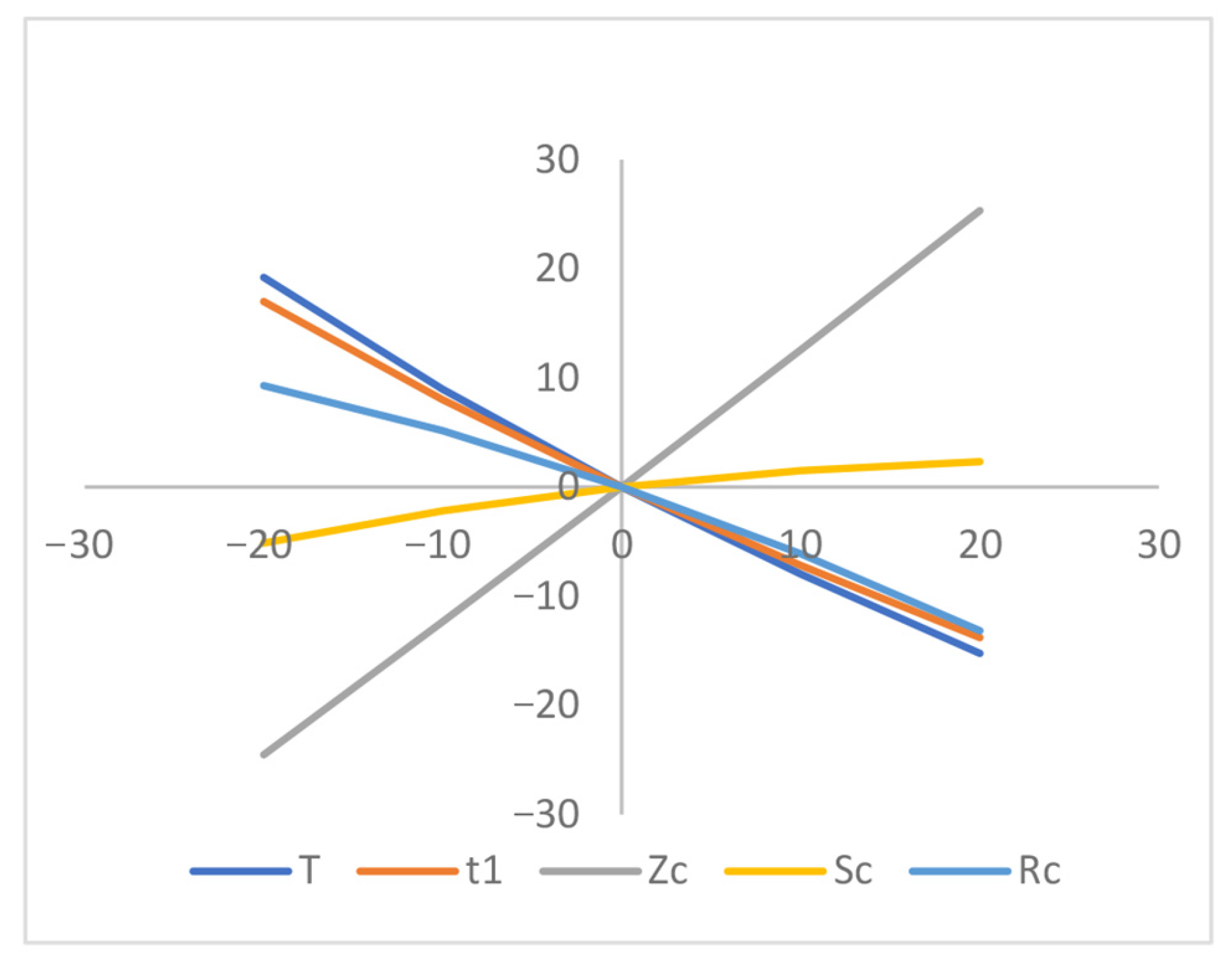
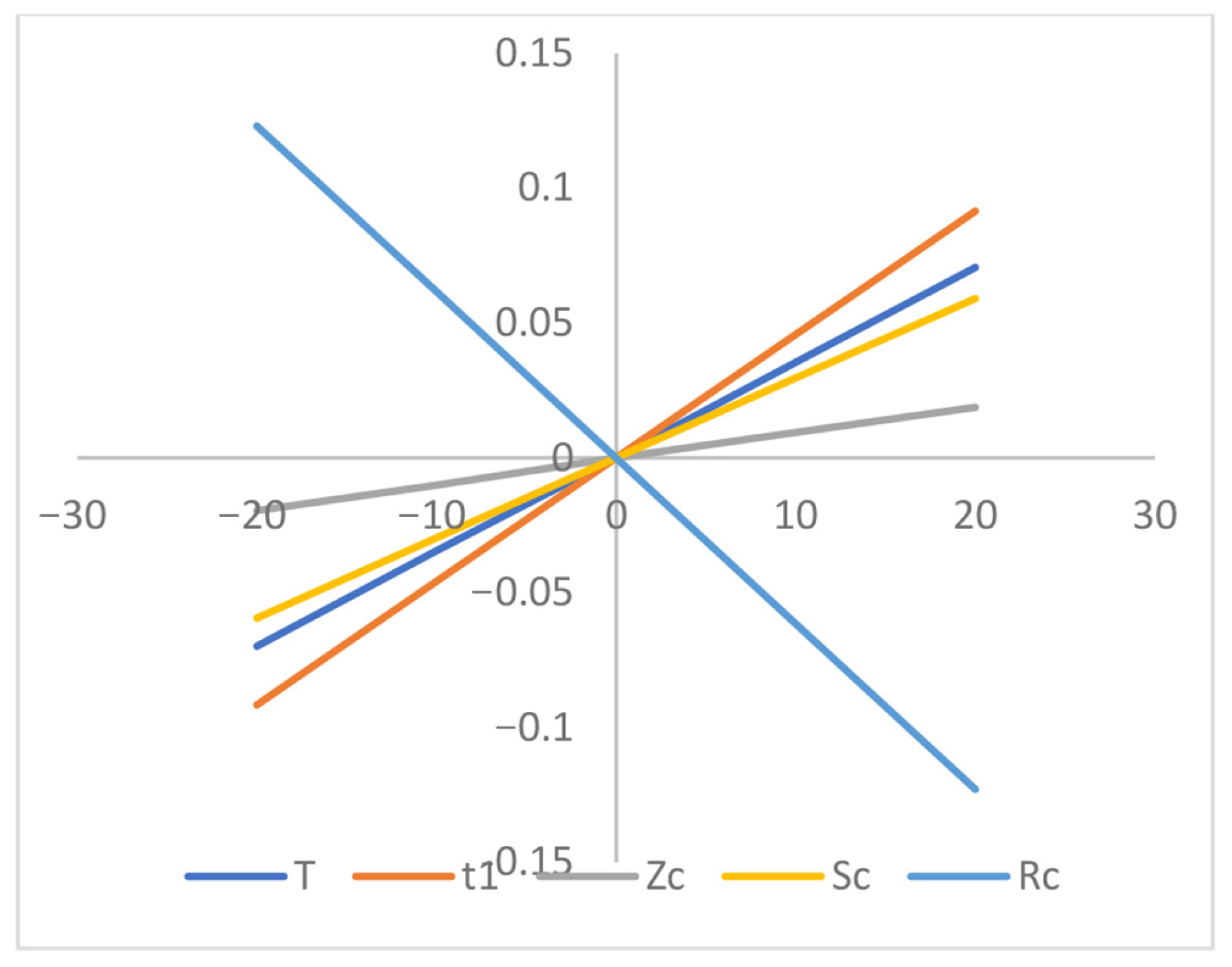
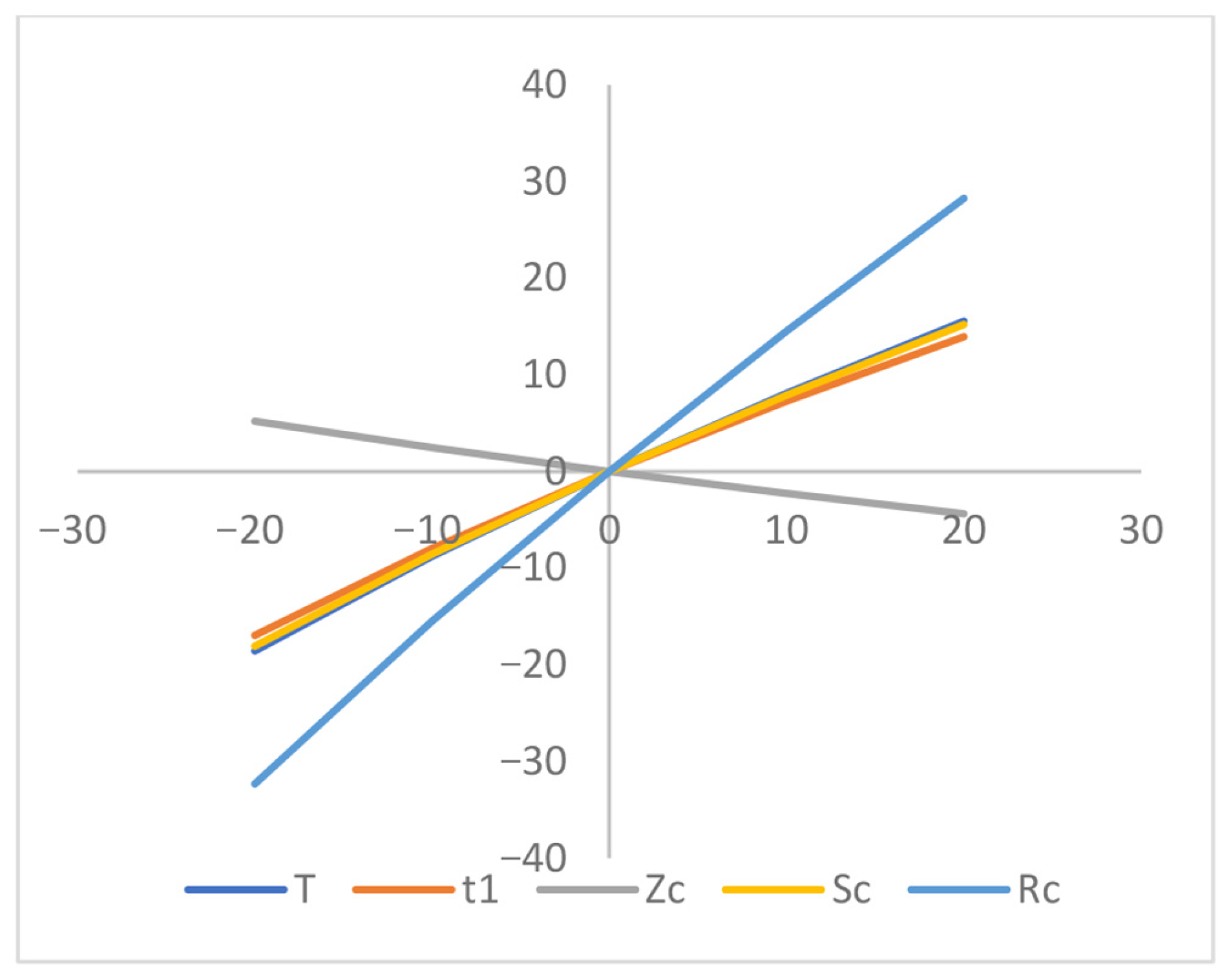
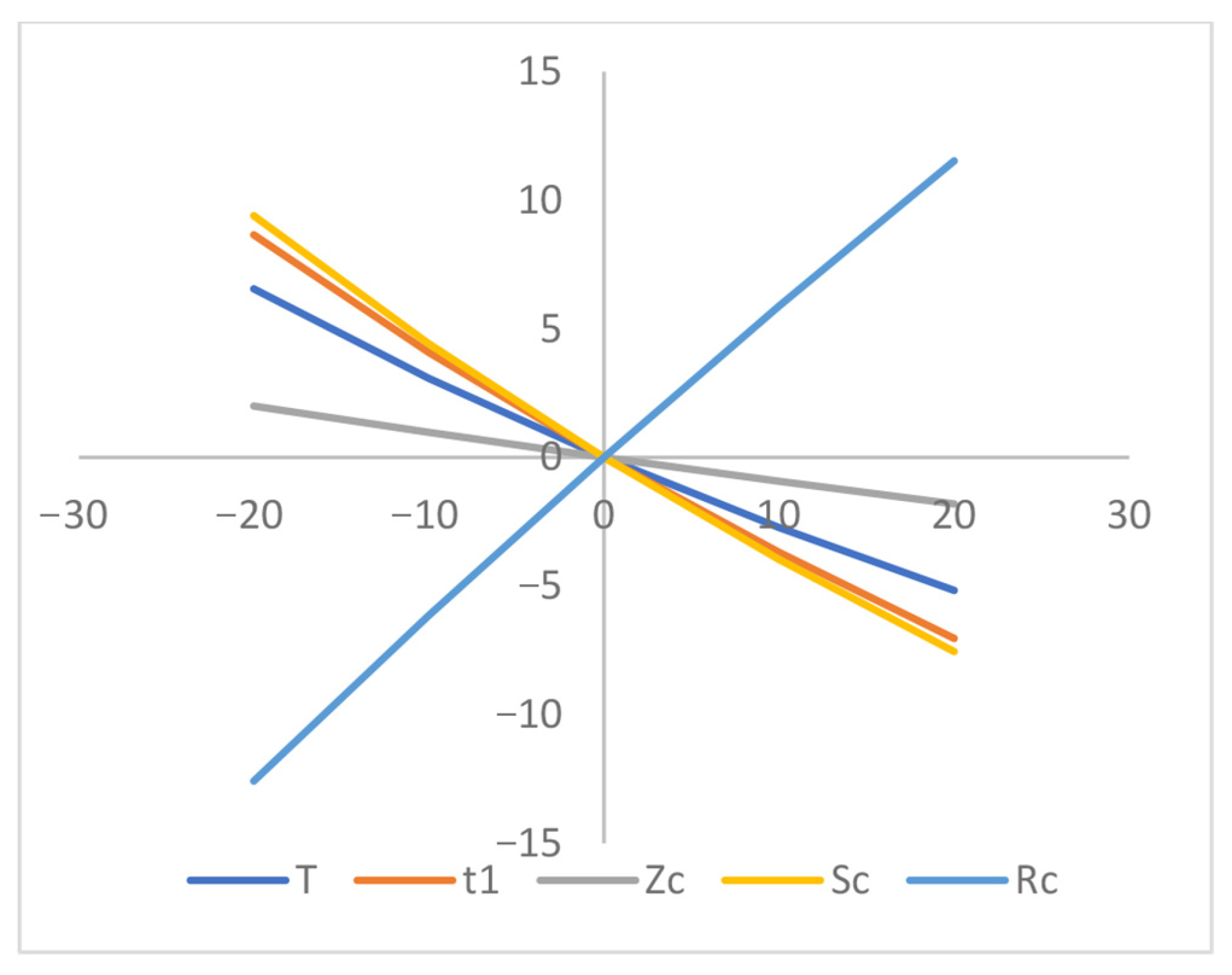
Note: For clarity in all Table 3 and Table 4 and Figure 2, Figure 3, Figure 4, Figure 5, Figure 6, Figure 7, Figure 8, Figure 9, Figure 10, Figure 11 and Figure 12, the units of measurement for each parameter are taken as follows:
  • Time-based variables: t 1 and T  are measured in time units (months);
  • Stock variables: [ S L , S U ] and [ R L , R U ]  are measured in units of product (Quintal);
  • Profit function: [ Z L , Z U ] ,     Z c  is measured in $/unit

6. Sensitivity Analysis

To demonstrate the influence of diverse system parameters on the stock-in period ( t 1 ), business cycle length (T), initial stock level ( [ S L , S U ] ), maximum shortage ( [ R L , R U ] ), and the center of average profit ( Z c , senitivity analyses are conducted. Since parameters differ in dimensions, each variable has been normalized during sensitivity analysis to allow comparison on a common scale. This ensures that variations in time, quantity, and profit are visually comparable within the same figure.
These analyses are carried out concerning numerical Example 2 by varying the parameter values from −20% to +20%. The optimal outcomes of these analyses are numerically depicted in Figure 5, Figure 6, Figure 7, Figure 8, Figure 9, Figure 10, Figure 11 and Figure 12.
  • Based on the sensitivity analyses depicted in Figure 5, Figure 6, Figure 7, Figure 8, Figure 9, Figure 10, Figure 11 and Figure 12, the center of the average profit ( Z c ) exhibits high sensitivity with respect to p, a L , a U , b L , b U . However, the parameter demonstrates a reverse effect compared to parameter. Alternatively it shows less sensitivity to k 0 L , k 0 U , [ h L , h U ] , and r L , r U , whereas it demonstrates insensitivity to changes in ‘ θ L , θ U ’ and ‘ α ’.
  • Figure 5, Figure 6, Figure 7, Figure 8, Figure 9, Figure 10, Figure 11 and Figure 12 illustrate that the business length ( T ) and the maximum shortage level, S L , S U are highly sensitive a L , a U . Both T and S L , S U demonstrate nearly equal sensitivity to k 0 L , k 0 U and b L , b U , respectively. Additionally, both T and S L , S U exhibit lower sensitivity to p, θ L , θ U ) and [ h L , h U ] , but parameters b L , b U and θ L , θ U show a reverse effect. Furthermore, both T and S L , S U are insensitive to positive or negative changes in ‘ α ’, ‘ b L , b U ’ and ‘ r L , r U , respectively.
  • The maximum interval-valued shortage level ( R L , R U ) is heavily sensitive with the changes of ‘ k 0 L , k 0 U ’, ‘ b L , b U ’ and ‘p’ and it is slightly affected with respect to ‘ a L , a U ’, ‘ θ L , θ U ’ and ‘ [ h L , h U ] ’, respectively. The shortage level ( R L , R U ) is much less sensitive with respect to ‘ r L , r U ’, whereas ‘ R L , R U ’ is insensitive with the changes in preservation rate parameter ‘ α ’.

7. Managerial Insights

The proposed IEQ model can assist business managers in making effective inventory decisions when demand, cost, or other parameters are uncertain. It converts theoretical modeling into an easy-to-use, decision-support tool that helps balance order quantity, preservation investment, and financial planning under real-world ambiguity.
In many industries—such as food retail, pharmaceuticals, and agriculture—product’s demand, prices, and deterioration rates are rarely fixed. The IEOQ model allows managers to input these uncertain factors as intervals rather than single values. The model then provides a profit range (lower and upper bounds) instead of one fixed number, helping firms make safer and more informed decisions. By using the C-U optimization technique, businesses can identify the combination of order size, cycle length, and payment strategy that yields the most stable and profitable outcome, even when exact data are unavailable.
Step-by-step guideline
  • Identify uncertain inputs (demand rate, deterioration rate, inventory cost, discount, etc.) and define their lower and upper bounds.
  • Formulate the IEOQ model using interval differential equations and interval parametric approach.
  • Apply the C–U optimization to obtain optimal order quantity, cycle time, and profit interval.
  • Interpret the results—the center value gives expected profit, and the upper bound indicates the best outcome.
  • Use sensitivity analysis to see how changes in key factors affect profit and policy decisions.
This approach offers a simple, structured way for practitioners to handle uncertainty, plan safe inventory levels, and make financially sound decisions in complex real-world settings.

8. Concluding Remarks

In summary, this study has studied optimizing business strategies within an interval inventory model framework, incorporating preservation technology, advanced payment methods, and fixed discounts, all facilitated by the C-U optimization approach. The notable findings of this work reveal that employing the C-U optimization method yields robust strategies for maximizing profit within this uncertain environment. Furthermore, numerical analyses have demonstrated that the optimal average profit obtained from the interval inventory model consistently encompasses the range of profits derived from the corresponding crisp model, reaffirming the model’s robustness and practical utility.
By integrating multiple business strategies into an interval-based optimization, this work advances the theoretical understanding of inventory management under uncertainty. The use of proposed C-U optimization method highlights its effectiveness in deriving strong decision-making strategies that outperform traditional crisp approaches. The model assumes a single-echelon structure with static deterioration and discount rates to preserve analytical tractability. However, the study has few limitations. Firstly, it is sometimes difficult to determine the bounds of the interval-valued parameters due to the high fluctuations of the imprecise parameters. Secondly, the parameter intervals used in the numerical examples were benchmarked from the existing literature rather than calibrated with primary or statistically validated data. This choice maintains methodological focus but limits the model’s empirical precision. Finally, the model assumes static deterioration and discount rates within a single-echelon structure, which simplifies computation but does not capture the dynamic and heterogeneous nature of real retail systems.
Future research could extend the model to address more complex forms of uncertainty, such as stochastic or fuzzy or Type-2 interval environments to enhance flexibility and adaptability in decision-making. Exploring dynamic extensions, multi-product settings, and integration with sustainability considerations could further enrich the model’s applicability. Such directions would strengthen the practical value of interval optimization approaches and contribute to more informed and adaptive business practices.

Funding

This research received no external funding.

Data Availability Statement

The original contributions presented in this study are included in the article. Further inquiries can be directed to the corresponding author.

Acknowledgments

The author is thankful to the Editor and reviewers for their constructive suggestions and comments to improve the paper.

Conflicts of Interest

The author declares that he has no conflicts of interest.

Appendix A

In this section, we have presented preliminary concepts of parametric representation of intervals (Ramezanadeh et al. [41]) with arithmetic operations between intervals in parametric form.

Appendix A.1. Arithmetic of Intervals

Let K c be the space of nonempty closed and bounded intervals of , i.e., K c = a L , a U : a L , a U .
Let A = a L , a U K c ,     where   a L   and   a U are the lower and upper bounds of A , respectively. Then, parametric representations of A are as follows:
(ii)
A = a r : a r = a L + r a U a L ,   r 0 , 1 (Increasing representation or IR),
(ii)
A = a r : a r = a U r a U a L ,   r 0 , 1 (Decreasing representation or DR).
Definition A1.
Let  a r : r 0 , 1     a n d   b r : r 0 , 1  be the IRs (DRs) of  A = a L , a U       and   B = b L , b U , respectively, and  λ  be a real number. Then parametric arithmetic in  K c  is defined as follows:
( i ) A + B = a r 1 + b r 2 : r 1 , r 2 0 , 1 , ( i i ) A . B = a r 1 b r 2 : r 1 , r 2 0 , 1 , ( i i i ) A / B = a r 1 / b r 2 : b r 2 0 , r 1 , r 2 0 , 1 , ( i v ) λ . A = λ a r 1 : r 1 0 , 1 , ( v ) A p B = a r b r : r 0 , 1 , ( v i ) A = B a r : r 0 , 1 = b r : r 0 , 1 .

Appendix A.2. Parametric Representation of Interval-Valued Function

Let F : D K c be an interval-valued function with lower and upper bounds form, F x = f L x , f U x . Then parametric representations of F x     are
( a )   f L x + r f U x f L x : r 0 , 1 ( b )   f U x r f U x f L x : r 0 , 1
Definition A2.
Let  F : D K c  be an interval-valued function and  x o D .     L K c  is the limit of  F   at   x o ,   if for every  ε > 0 ,   δ > 0     such   that     d p F x , L < ε ,  whenever  0 < x x o < δ ,   and   it   is   denoted   by   lim x x o F x = L .
Where
d p A , B = max min r a r b r , max r a r b r , A = a r | r 0 , 1 , B = b r | r 0 , 1
Proposition A1.
 
    F x = f x , r | f : D ; r 0 , 1 k   is   continuous   at   x o D   iff   f x , r   is   continuousat   x o ,   for   all   r 0 , 1 k ,   where     k   be   the   number   of   interval   coefficients   in   F .  
Definition A3.
The P-derivative of an interval-valued function  F : D K c  at the point  x o D .      is denoted by  F x o  and is defined by  F x o = lim h 0 F x o + h p F x o h .
  • where h   is   such   that   x o + h D .   In   this   case ,   F   is   called   p - differentiable   at   x o .
Proposition A2.
 
  The   interval - valued   function   F x = f x , r | f : D ; r 0 , 1 k is   p - differentiable   at   x o Diff   for   all   r 0 , 1 k ,   f x , r   is   differentiable   at   x o   and   F x o = f x o , r | f : D ; r 0 , 1 k
Definition A4.
Let  a , b D .  Then the definite integral  a b F x d x  of an interval-valued function  F x = f x , r | f : D , r 0 , 1 k  is defined by a b F x d x = a b f x , r d x |   f x , r   is   integrable   w . r . t   x   r 0,1 k .

References

  1. Tayal, S.; Singh, S.R.; Sharma, R.; Chauhan, A. Two echelon supply chain model for deteriorating items with effective investment in preservation technology. Int. J. Math. Oper. Res. 2014, 6, 84–105. [Google Scholar] [CrossRef]
  2. Dye, C.Y.; Yang, C.T. Optimal dynamic pricing and preservation technology investment for deteriorating products with reference price effects. Omega 2016, 62, 52–67. [Google Scholar] [CrossRef]
  3. Panda, G.C.; Khan, M.A.A.; Shaikh, A.A. A credit policy approach in a two-warehouse inventory model for deteriorating items with price-and stock-dependent demand under partial backlogging. J. Ind. Eng. Int. 2019, 15, 147–170. [Google Scholar] [CrossRef]
  4. Adak, S.; Mahapatra, G.S. Effect of reliability on multi-item inventory system with shortages and partial backlog incorporating time dependent demand and deterioration. Ann. Oper. Res. 2020, 315, 1551–1571. [Google Scholar] [CrossRef]
  5. San-José, L.A.; Sicilia, J.; González-De-la-Rosa, M.; Febles-Acosta, J. Optimal inventory policy under power demand pattern and partial backlogging. Appl. Math. Model. 2017, 46, 618–630. [Google Scholar] [CrossRef]
  6. Rahman, M.S.; Khan, M.A.A.; Halim, M.A.; Nofal, T.A.; Shaikh, A.A.; Mahmoud, E.E. Hybrid price and stock dependent inventory model for perishable goods with advance payment related discount facilities under preservation technology. Alex. Eng. J. 2021, 60, 3455–3465. [Google Scholar] [CrossRef]
  7. Xu, C.; Zhao, D.; Min, J.; Hao, J. An inventory model for nonperishable items with warehouse mode selection and partial backlogging under trapezoidal-type demand. J. Oper. Res. Soc. 2020, 72, 744–763. [Google Scholar] [CrossRef]
  8. Karmakar, B. Inventory models with ramp-type demand for deteriorating items with partial backlogging and time-varing holding cost. Yugosl. J. Oper. Res. 2016, 24, 249–266. [Google Scholar] [CrossRef]
  9. Yadav, A.S.; Swami, A. A partial backlogging production-inventory lot-size model with time-varying holding cost and Weibull deterioration. Int. J. Procure. Manag. 2018, 11, 639–649. [Google Scholar]
  10. Soto, A.V.; Chowdhury, N.T.; Allahyari, M.Z.; Azab, A.; Baki, M.F. Mathematical modeling and hybridized evolutionary LP local search method for lot-sizing with supplier selection, inventory shortage, and quantity discounts. Comput. Ind. Eng. 2017, 109, 96–112. [Google Scholar] [CrossRef]
  11. Taleizadeh, A.A. Lot-sizing model with advance payment pricing and disruption in supply under planned partial backordering. Int. Trans. Oper. Res. 2017, 24, 783–800. [Google Scholar] [CrossRef]
  12. Shaikh, A.A.; Das, S.C.; Bhunia, A.K.; Panda, G.C.; Khan, M.A.A. A two-warehouse EOQ model with interval-valued inventory cost and advance payment for deteriorating item under particle swarm optimization. Soft Comput. 2019, 23, 13531–13546. [Google Scholar] [CrossRef]
  13. Khan, M.A.A.; Shaikh, A.A.; Panda, G.C.; Konstantaras, I.; Cárdenas-Barrón, L.E. The effect of advance payment with discount facility on supply decisions of deteriorating products whose demand is both price and stock dependent. Int. Trans. Oper. Res. 2020, 27, 1343–1367. [Google Scholar] [CrossRef]
  14. Taleizadeh, A.A.; Zarei, H.R.; Sarker, B.R. An optimal control of inventory under probablistic replenishment intervals and known price increase. Eur. J. Oper. Res. 2017, 257, 777–791. [Google Scholar] [CrossRef]
  15. Mondal, R.; Shaikh, A.A.; Bhunia, A.K. Crisp and interval inventory models for ameliorating item with Weibull distributed amelioration and deterioration via different variants of quantum behaved particle swarm optimization-based techniques. Math. Comput. Model. Dyn. Syst. 2019, 25, 602–626. [Google Scholar] [CrossRef]
  16. Rahaman, M.; Alam, S.; Alamin, A.; Mondal, S.P.; Singh, P. An application of intuitionistic fuzzy differential equation to the inventory model. In Fuzzy Optimization, Decision-Making and Operations Research: Theory and Applications; Springer International Publishing: Cham, Switzerland, 2023; pp. 679–702. [Google Scholar]
  17. Sadeghi, J.; Mousavi, S.M.; Niaki, S.T.A. Optimizing an inventory model with fuzzy demand, backordering, and discount using a hybrid imperialist competitive algorithm. Appl. Math. Model. 2016, 40, 7318–7335. [Google Scholar] [CrossRef]
  18. Ghorabaee, M.K.; Amiri, M.; Zavadskas, E.K.; Turskis, Z.; Antucheviciene, J. A new multi-criteria model based on interval type-2 fuzzy sets and EDAS method for supplier evaluation and order allocation with environmental considerations. Comput. Ind. Eng. 2017, 112, 156–174. [Google Scholar] [CrossRef]
  19. Mondal, S.P. Solution of Basic Inventory Model in Fuzzy and Interval Environments: Fuzzy and Interval Differential Equation Approach. In Handbook of Research on Fuzzy and Rough Set Theory in Organizational Decision Making; IGI Global: Hershey, PA, USA, 2017; pp. 65–95. [Google Scholar]
  20. Shaikh, A.A.; Bhunia, A.K.; Cárdenas-Barrón, L.E.; Sahoo, L.; Tiwari, S. A fuzzy inventory model for a deteriorating item with variable demand, permissible delay in payments and partial backlogging with shortage follows inventory (SFI) policy. Int. J. Fuzzy Syst. 2018, 20, 1606–1623. [Google Scholar] [CrossRef]
  21. Bhunia, A.K.; Shaikh, A.A. Investigation of two-warehouse inventory problems in interval environment under inflation via particle swarm optimization. Math. Comput. Model. Dyn. Syst. 2016, 22, 160–179. [Google Scholar] [CrossRef]
  22. Bhunia, A.K.; Shaikh, A.A.; Cárdenas-Barrón, L.E. A partially integrated production-inventory model with interval-valued inventory costs, variable demand and flexible reliability. Appl. Soft Comput. 2017, 55, 491–502. [Google Scholar] [CrossRef]
  23. Kumar, P.; Keerthika, P.S. An inventory model with variable holding cost and partial backlogging under interval uncertainty: Global criteria method. Int. J. Mech. Eng. Technol. 2018, 9, 1567–1578. [Google Scholar]
  24. Ruidas, S.; Seikh, M.R.; Nayak, P.K.; Sarkar, B. A single period production inventory model in interval environment with price revision. Int. J. Appl. Comput. Math. 2019, 5, 7. [Google Scholar] [CrossRef]
  25. Shaikh, A.A.; Cárdenas-Barrón, L.E.; Tiwari, S. A two-warehouse inventory model for non-instantaneous deteriorating items with interval-valued inventory costs and stock-dependent demand under inflationary conditions. Neural Comput. Appl. 2019, 31, 1931–1948. [Google Scholar] [CrossRef]
  26. Rahman, M.S.; Duary, A.; Shaikh, A.A.; Bhunia, A.K. An application of parametric approach for interval differential equation in inventory model for deteriorating items with selling-price-dependent demand. Neural Comput. Appl. 2020, 32, 14069–14085. [Google Scholar] [CrossRef]
  27. Rahman, M.S.; Manna, A.K.; Shaikh, A.A.; Bhunia, A.K. An application of interval differential equation on a production inventory model with interval-valued demand via center-radius optimization technique and particle swarm optimization. Int. J. Intell. Syst. 2020, 35, 1280–1326. [Google Scholar] [CrossRef]
  28. Rahman, M.S.; Duary, A.; Khan, M.A.A.; Shaikh, A.A.; Bhunia, A.K. Interval-valued demand related inventory model under all units discount facility and deterioration via parametric approach. Artif. Intell. Rev. 2022, 55, 2455–2494. [Google Scholar] [CrossRef]
  29. Cuevas, E.; Rodríguez, A.; Alejo-Reyes, A.; Del-Valle-Soto, C. Metaheuristic Algorithms Applied to the Inventory Problem. In Recent Metaheuristic Computation Schemes in Engineering; Springer International Publishing: Cham, Switzerland, 2021; pp. 237–277. [Google Scholar]
  30. Sajadi, S.J.; Ahmadi, A. An integrated optimization model and metaheuristics for assortment planning, shelf space allocation, and inventory management of perishable products: A real application. PLoS ONE 2022, 17, e0264186. [Google Scholar] [CrossRef]
  31. Huang, B. Metaheuristic-Based Supply Chain Network Optimization and Inventory Management Using Ant Colony Algorithm. Informatica 2025, 49, 17–32. [Google Scholar] [CrossRef]
  32. de Paula Vidal, G.H.; Caiado, R.G.G.; Scavarda, L.F.; Ivson, P.; Garza-Reyes, J.A. Decision support framework for inventory management combining fuzzy multicriteria methods, genetic algorithm, and artificial neural network. Comput. Ind. Eng. 2022, 174, 108777. [Google Scholar] [CrossRef]
  33. Saha, C.; Jana, D.K.; Duary, A. Enhancing production inventory management for imperfect items using fuzzy optimization strategies and Differential Evolution (DE) algorithms. Frankl. Open 2023, 5, 100051. [Google Scholar] [CrossRef]
  34. Manna, A.K.; Bhunia, A.K. Investigation of green production inventory problem with selling price and green level sensitive interval-valued demand via different metaheuristic algorithms. Soft Comput. 2022, 26, 10409–10421. [Google Scholar] [CrossRef]
  35. Duary, A.; Rahman, M.S.; Manna, A.K.; Shaikh, A.A. Optimal policy of an interval production problem with variable demand and warranty policy via 0 _ 1 parametrized optimization technique. Int. J. Syst. Assur. Eng. Manag. 2025, 16, 2967–2982. [Google Scholar] [CrossRef]
  36. Mashud, A.H.M.; Wee, H.M.; Sarkar, B.; Li, Y.H.C. A sustainable inventory system with the advanced payment policy and trade-credit strategy for a two-warehouse inventory system. Kybernetes 2020, 50, 1321–1348. [Google Scholar] [CrossRef]
  37. Saren, S.; Sarkar, B.; Bachar, R.K. Application of various price-discount policy for deteriorated products and delay-in-payments in an advanced inventory model. Inventions 2020, 5, 50. [Google Scholar] [CrossRef]
  38. Mondal, R.; Das, S.; Das, S.C.; Shaikh, A.A.; Bhunia, A.K. Pricing strategies and advance payment-based inventory model with partially backlogged shortages under interval uncertainty. Int. J. Syst. Sci. Oper. Logist. 2023, 10, 2070296. [Google Scholar] [CrossRef]
  39. Akhtar, F.; Khan, M.A.A.; Shaikh, A.A.; Alrasheedi, A.F. Interval-valued inventory model for deterioration, carbon emissions and selling price dependent demand considering buy now and pay later facility. Ain Shams Eng. J. 2024, 15, 102563. [Google Scholar] [CrossRef]
  40. Yadav, K.K.; Yadav, A.S.; Bansal, S. Interval number approach for two-warehouse inventory management of deteriorating items with preservation technology investment using analytical optimization methods. Int. J. Interact. Des. Manuf. (IJIDeM) 2024, 1–17. [Google Scholar] [CrossRef]
  41. Ramezanadeh, M.; Heidari, M.; Fard, O.S.; Borzabadi, A.H. On the interval differential equation: Novel solution methodology. Adv. Differ. Equ. 2015, 2015, 338. [Google Scholar] [CrossRef]
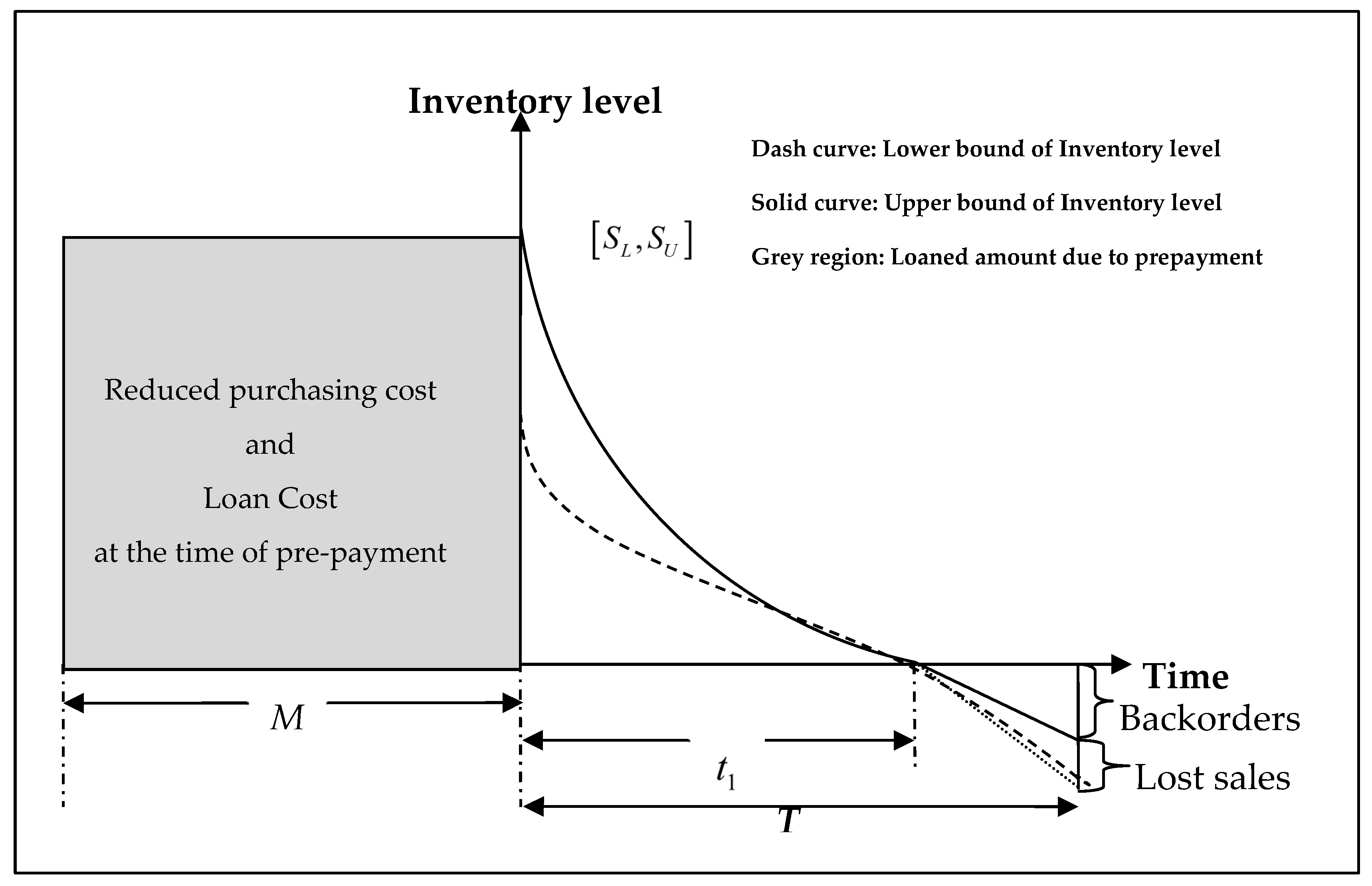
Figure 1. Varying the inventory system with full prepayment, accounting for partially backlogged shortages (all the symbols have their own meaning, presented in Table 2).
Appliedmath 05 00151 g001
Figure 2. Range of average profit for Example 1.
Appliedmath 05 00151 g002
Figure 3. Center of the average profit of Example 1.
Appliedmath 05 00151 g003
Figure 4. Concavity of average profit function.
Appliedmath 05 00151 g004
Figure 5. Effect on the optimality due to a L , a U .
Appliedmath 05 00151 g005
Figure 6. Effect on the optimality due to b L , b U .
Appliedmath 05 00151 g006
Figure 7. Effect on the optimality due to θ L , θ U .
Appliedmath 05 00151 g007
Figure 8. Effect on the optimality due to r L , r U .
Appliedmath 05 00151 g008
Figure 9. Effect on the optimality due to α .
Appliedmath 05 00151 g009
Figure 10. Effect on the optimality due to p .
Appliedmath 05 00151 g010
Figure 11. Effect on the optimality due to [ K o L , K o U ] .
Appliedmath 05 00151 g011
Figure 12. Effect on the optimality due to [ h L , h U ] .
Appliedmath 05 00151 g012
Table 1. Comparison table of related works.
Related WorksDemandDiscount PolicyAdvanced PaymentPreservation TechnologyBackloggingGoverning Differential EquationsSolution Procedure
Dye and Yang [1]variableNoNoYesNoCrispAnalytically
Shaikh et al. [20]variableNoNoNoYesFuzzyAnalytically
Shaikh et al. [25]variableNoYesNoNoIntervalPSO
Mashud et al. [36]variableNoYesNoNoCrispAnalytically/Numerically
Saren et al. [37]variableYesNoNoNoCrispAnalytically
Rahman et al. [26]Interval-valued and price-dependentNoNoNoNoIntervalQPSO
Mondal et al. [38]Interval-valued and price-dependentNoYesNoYesIntervalSoft-computing
Akhtar et al. [39]Interval-valued and priceNoNoNoYesIntervalSoft-computing
Yadav et al. [40]timeNoNoYesYesIntervalAnalytical
N.B. PSO: Particle Swarm Optimization, QPSO: Quantum-behaved PSO.
Table 2. Useful notation and description.
SymbolsUnitsDescriptions
I 1 L t , I 1 U t UnitsInterval-valued inventory level where 0 t t 1
I 2 L t , I 2 U t UnitsInterval-valued inventory level t where t 1 t T
D L p , D U p Per unitsInterval-valued demand rate
Q L , Q U UnitsInterval-valued order size per cycle
S L , S U UnitsInterval-valued highest stock level
R L , R U UnitsInterval-valued maximum shortages level
θ L , θ U ConstantInterval-valued deterioration rate
η L , η U ConstantInterval-valued backlogging rate
M Time unitPrepayment period
α L , α U ,   β L , β U UnitsInterval-valued parameters in linear part of demand
a L , a U ,   b L , b U UnitsInterval-valued parameters in nonlinear part of demand
α UnitsPreservation technology scaling parameter
r L , r U %Interval-valued percentage discount applied to the total purchasing cost
K o L , K o U $/orderInterval-valued restocking cost
C i L , C i U $/unitInterval-valued purchasing cost
h L , h U ,   g L , g U $/unit/time unitParameters of interval-valued holding cost
C s L , C s U $/unit/time unitInterval-valued shortages cost
C d L , C d U $/unitInterval-valued deterioration cost
C l L , C l U $/unitInterval-valued opportunity cost
I e L , I e U $/time unitInterval-valued cost of loan rate
π L t 1 , T , π U t 1 , T $/time unitInterval-valued the total cost
σ L , σ U $/unitInterval-valued preservation cost
p $/unitSelling price
Decision variables
t 1 Time unitStock-in time
TTime unitBusiness cycle
Table 3. C-U optimal solution with respect to Example 1.
VariablesC-U Optimal Values
T 1.12016
t 1 0.895745
[ Z L , Z U ] [459.324, 1827.99]
[ S L , S U ] [32.4868, 46.1317]
[ R L , R U ] [5.75245, 11.2361]
Table 4. C-U Optimal solution with respect to Example 2.
VariablesC-U Optimal Values
T 1.15994
t 1 1.04871
Z L , Z U [1278.96, 1278.96]
S L , S U [45.8497, 45.8497]
R L , R U [4.22362, 4.22362]
Disclaimer/Publisher’s Note: The statements, opinions and data contained in all publications are solely those of the individual author(s) and contributor(s) and not of MDPI and/or the editor(s). MDPI and/or the editor(s) disclaim responsibility for any injury to people or property resulting from any ideas, methods, instructions or products referred to in the content.