Analytic Solutions and Conservation Laws of a 2D Generalized Fifth-Order KdV Equation with Power Law Nonlinearity Describing Motions in Shallow Water Under a Gravity Field of Long Waves

Abstract

The Korteweg–de Vries (KdV) equation is a nonlinear evolution equation that reflects a wide variety of dispersive wave occurrences with limited amplitude. It has also been used to describe a range of major physical phenomena, such as shallow water waves that interact weakly and nonlinearly, acoustic waves on a crystal lattice, lengthy internal waves in density-graded oceans, and ion acoustic waves in plasma. The KdV equation is one of the most well-known soliton models, and it provides a good platform for further research into other equations. The KdV equation has several forms. The aim of this study is to introduce and investigate a (2+1)-dimensional generalized fifth-order KdV equation with power law nonlinearity (gFKdVp). The research methodology employed is the Lie group analysis. Using the point symmetries of the gFKdVp equation, we transform this equation into several nonlinear ordinary differential equations (ODEs), which we solve by employing different strategies that include Kudryashov’s method, the $(G^{\prime }/G)$ expansion method, and the power series expansion method. To demonstrate the physical behavior of the equation, 3D, density, and 2D graphs of the obtained solutions are presented. Finally, utilizing the multiplier technique and Ibragimov’s method, we derive conserved vectors of the gFKdVp equation. These include the conservation of energy and momentum. Thus, the major conclusion of the study is that analytic solutions and conservation laws of the gFKdVp equation are determined.

1. Introduction

Over the years, the construction of mathematical models has aided in the effective description of a variety of physical processes in engineering, finance, and natural sciences. Nonlinear partial differential equations (PDEs) typically represent the important physical processes of the model, including genetic engineering, the spread of infectious diseases, the behavior of tidal waves, the pricing of derivatives, and many others. For instance, the Shigesada–Kawasaki–Teramoto cross-diffusion model was investigated in [1] to prove the existence of global weak solutions for an arbitrary number of species. Also, the authors of [2] studied the shallow water wave equation, which is mostly used in fluid mechanics as the model that describes the flow of fluids below a pressured surface. In [3], a nonlinear (1+1)-dimensional fifth-order equation was examined and multiple soliton solutions were obtained. In addition, the authors of [4] studied the new extended (3+1)-dimensional Boussinesq equation and obtained multiple soliton solutions, soliton molecules, and travelling wave solutions of the equation.

To comprehend these physical processes, we must seek the exact solutions of these nonlinear PDEs. Thus, one of the major topics in mathematical physics is finding exact solutions to nonlinear PDEs that appear in many physical applications. Most of the time, finding exact solutions to these equations is challenging.

Currently, there is no efficient method for finding the general solution of nonlinear PDEs, although there are methodologies and mathematical tools that have been developed by researchers that may help in finding a specific type of solution. In this paper, our attention is focused on employing Lie group analysis [5,6] to find analytic solutions. A point symmetry of a differential equation (DE) is a transformation that maps solutions of the DE to other solutions of the same DE. Once symmetry of the DE is found, one may use it to lower the order of the DE. This process is called symmetry reduction. Several researchers have successfully introduced methods for finding specific analytic solutions to nonlinear PDEs. These include the Hirota method [7], Cole–Hopf transformation approach [8], extended simplest equation technique [9], symmetry method [10], neural network method [11], Mittag–Leffler kernel technique [12], modified simple equation method [13], Fokas method [14], hybrid technique for improved accuracy [15], extended homoclinic test approach [16], sine-Gordon equation expansion technique [17], $(G^{\prime }/G)-$ expansion method [18], power series solution technique [19], Painlevé expansion technique [20], tanh–coth technique [21], the mapping approach [22], homotopy perturbation technique [23], generalized extended rational expansion method [24], Kudryashov method [25], and Bäcklund transformation technique [26].

Lu et al. [27] considered the $(2+1)$-dimensional generalized fifth-order Korteweg–de Vries (KdV) equation

$$\alpha u_{xxxxx}+\beta u{u}_{xxx}+\gamma u_x{u}_{xx}+\delta u^2{u}_x+u_t+u_y=0,$$

(1)

where $\alpha ,\beta ,\gamma$, and $\delta$ are the coefficients of the fifth-order dispersion term and high-order nonlinear term, which are arbitrary nonzero real numbers. Equation (1) describes motions of long waves in shallow water under a gravity field and in a two-dimensional nonlinear lattice. The variables t and x represent time and space, respectively. In Equation (1), the authors took $\alpha =1$, $\beta =\gamma =15$, and $\delta =45$ and obtained the equation

$$u_{xxxxx}+15u{u}_{xxx}+15u_x{u}_{xx}+45u^2{u}_x+u_t+u_y=0.$$

(2)

Furthermore, upon solving Equation (2) using the Hirota bilinear method, a kind of lump solution and two classes of interaction were discussed [27].

Moreover, new solutions were found in [28] by employing the Hirota bilinear form and the authors investigated the interactions between the lump-type solutions and the double exponential functions.

Lastly, Guo et al. [29] used the Hirota bilinear forms with the Hirota direct method and, as a result, the single soliton and the single periodic wave solutions were obtained.

In this paper, we further generalize Equation (2) and obtain the (2+1)-dimensional generalized fifth-order Korteweg–de Vries equation with power law nonlinearity (gFKdVp) equation

$$u_{xxxxx}+au{u}_{xxx}+a{u}_x{u}_{xx}+3a{u}^n{u}_x+u_t+u_y=0,$$

(3)

where a is an arbitrary nonzero real number and n is a nonzero constant.

With a motivation to expand the area of applications of Equation (3), we employ Lie group analysis to obtain new analytic solutions. To the best of our knowledge, the results obtained in this paper are new and have not been reported.

The rest of the paper is organized as follows. Lie point symmetries are obtained in Section 2. In Section 3, we construct conserved vectors of Equation (3) using the general multiplier methodology and Ibragimov’s method. Symmetry reductions of Equation (3) are performed and, thereafter, analytic solutions are constructed in Section 4. Also, dynamical behavior of certain solutions are depicted. Finally, in Section 5, concluding remarks are given.

2. Point Symmetries of (3)

First and foremost, Lie theory is used to compute point symmetries of the form

$$\begin{array}{c}\hfill \mathcal{S}=\tau {\displaystyle \frac{\partial }{\partial t}}+\xi {\displaystyle \frac{\partial }{\partial x}}+\varphi {\displaystyle \frac{\partial }{\partial y}}+\eta {\displaystyle \frac{\partial }{\partial u}},\end{array}$$

with coefficient functions $\tau ,\xi ,\varphi ,\eta$ depending on t, x, y, and u. Using the Lie invariance condition [30], the generator $\mathcal{S}$ is a symmetry of (3), provided

$${\mathcal{S}}^{\left[5\right]}{\mathit{\Delta }|}_{\mathit{\Delta }=0}=0,$$

(4)

holds with $\mathit{\Delta }=u_{xxxxx}+au{u}_{xxx}+a{u}_x{u}_{xx}+3a{u}^n{u}_x+u_t+u_y$. Here, ${\mathcal{S}}^{\left[5\right]}$ stands for the fifth extension of $\mathcal{S}$, given by

$$\begin{array}{c}\hfill {\displaystyle {\mathcal{S}}^{\left[5\right]}=\mathcal{S}+{\zeta }_1\frac{\partial }{\partial u_t}+{\zeta }_2\frac{\partial }{\partial u_x}+{\zeta }_3\frac{\partial }{\partial u_y}+{\zeta }_{22}\frac{\partial }{\partial u_{xx}}+{\zeta }_{222}\frac{\partial }{\partial u_{xxx}}+{\zeta }_{22222}\frac{\partial }{\partial u_{xxxxx}},}\end{array}$$

(5)

and ${\zeta }_1,{\zeta }_2,{\zeta }_3,{\zeta }_{22},{\zeta }_{222}$, and ${\zeta }_{22222}$ are determined by

$$\begin{array}{cc}\hfill {\zeta }_1=& D_t\left(\eta \right)-u_t{D}_t\left(\tau \right)-u_x{D}_t\left(\xi \right)-u_y{D}_t\left(\varphi \right),\hfill \\ \hfill {\zeta }_2=& D_x\left(\eta \right)-u_t{D}_x\left(\tau \right)-u_x{D}_x\left(\xi \right)-u_y{D}_x\left(\varphi \right),\hfill \\ \hfill {\zeta }_3=& D_y\left(\eta \right)-u_t{D}_y\left(\tau \right)-u_x{D}_y\left(\xi \right)-u_y{D}_y\left(\varphi \right),\hfill \\ \hfill {\zeta }_{22}=& D_x\left({\zeta }_2\right)-u_{tx}{D}_x\left(\tau \right)-u_{xx}{D}_x\left(\xi \right)-u_{xy}{D}_x\left(\varphi \right),\hfill \\ \hfill {\zeta }_{222}=& D_x\left({\zeta }_{22}\right)-u_{txx}{D}_x\left(\tau \right)-u_{xxx}{D}_x\left(\xi \right)-u_{xxy}{D}_x\left(\varphi \right),\hfill \\ \hfill {\zeta }_{22222}=& D_x\left({\zeta }_{2222}\right)-u_{txxxx}{D}_x\left(\tau \right)-u_{xxxxx}{D}_x\left(\xi \right)-u_{xxxxy}{D}_x\left(\varphi \right),\hfill \end{array}$$

with total derivatives $D_t$, $D_x$, and $D_y$, defined as

$$\begin{array}{cc}\hfill D_t=& {\displaystyle \frac{\partial }{\partial t}}+u_t{\displaystyle \frac{\partial }{\partial u}}+u_{tt}{\displaystyle \frac{\partial }{\partial u_t}}+u_{tx}{\displaystyle \frac{\partial }{\partial u_x}}+\dots ,\hfill \\ \hfill D_x=& {\displaystyle \frac{\partial }{\partial x}}+u_x{\displaystyle \frac{\partial }{\partial u}}+u_{tx}{\displaystyle \frac{\partial }{\partial u_t}}+u_{xx}{\displaystyle \frac{\partial }{\partial u_x}}+\dots ,\hfill \\ \hfill D_y=& {\displaystyle \frac{\partial }{\partial y}}+u_y{\displaystyle \frac{\partial }{\partial u}}+u_{ty}{\displaystyle \frac{\partial }{\partial u_t}}+u_{xy}{\displaystyle \frac{\partial }{\partial u_x}}+\dots .\hfill \end{array}$$

With the help of the scientific program Mathematica, expanding (4) and separating the derivatives of u, we obtain a system of linear homogeneous PDEs. Solving these equations yields

$$\tau =F^1(y-t),\xi =F^2(y-t),\varphi =F^3(y-t),\eta =0,$$

(6)

where $F^i,i=1,\dots ,3$ are arbitrary functions of their arguments. Thus, the point symmetries of the gFKdVp Equation (3) are given by:

$$\begin{array}{c}{\mathcal{S}}_1=F^1(y-t){\displaystyle \frac{\partial }{\partial t}},\hfill \\ {\mathcal{S}}_2=F^2(y-t){\displaystyle \frac{\partial }{\partial x}},\hfill \\ {\mathcal{S}}_3=F^3(y-t){\displaystyle \frac{\partial }{\partial y}}.\hfill \end{array}$$

The first symmetry represents the time translation, while the second and third symmetries are space translations. We obtain an extra fourth symmetry of Equation (3) when $n=2$, and it is given by

$$\begin{array}{c}{\mathcal{S}}_4=5F^4(y-t)t{\displaystyle \frac{\partial }{\partial t}}+F^4(y-t)x{\displaystyle \frac{\partial }{\partial x}}+5F^4(y-t)t{\displaystyle \frac{\partial }{\partial y}}-2F^4(y-t)u{\displaystyle \frac{\partial }{\partial y}}.\hfill \end{array}$$

3. Conservation Laws for (3)

The conserved vectors for the gFKdVp Equation (3) are computed in this section. To derive the conserved vectors, we apply two methods, namely the general multiplier technique and Ibragimov’s theorem.

3.1. Conserved Vectors via the Multiplier Approach

3.1.1. Conserved Vectors for (3)

We first compute the fourth-order multipliers $\mathcal{M}$, that is $\mathcal{M}$ depends on t, x, y, u, $u_x$, $u_{xx}$, $u_{xxx}$ and $u_{xxxx}$ [11] by using

$${\displaystyle \frac{\delta }{\delta u}}\left\{\mathcal{M}\left[u_{xxxxx}+au{u}_{xxx}+a{u}_x{u}_{xx}+3a{u}^n{u}_x+u_t+u_y\right]\right\}=0.$$

(7)

Here, $\delta /\delta u$ is a Euler operator that has the form

$${\displaystyle \frac{\delta }{\delta u}}={\displaystyle \frac{\partial }{\partial u}}-D_t{\displaystyle \frac{\partial }{\partial u_t}}-D_x{\displaystyle \frac{\partial }{\partial u_x}}-D_y{\displaystyle \frac{\partial }{\partial u_y}}+D_t{D}_x{\displaystyle \frac{\partial }{\partial u_{tx}}}-D_x^4{\displaystyle \frac{\partial }{\partial u_{xxxx}}}+D_t{D}_x^3{\displaystyle \frac{\partial }{\partial u_{txxx}}}+\dots ,$$

(8)

and $D_t,D_x$ and $D_y$ represent the total derivatives. The following seven linear determining equations are obtained by expanding (7):

$$\begin{array}{cc}\hfill & {\mathcal{M}}_t+{\mathcal{M}}_t=0,{\mathcal{M}}_x=0,{\mathcal{M}}_u=0,{\mathcal{M}}_{u_x}=0,{\mathcal{M}}_{u_{xx}}=0,{\mathcal{M}}_{u_{xxx}}=0,{\mathcal{M}}_{u_{xxxx}}=0,\hfill \end{array}$$

which, upon solving for $\mathcal{M}$, yields

$$\begin{array}{cc}\hfill & \mathcal{M}=F(y-t),\hfill \end{array}$$

(9)

where $F(y-t)$ is an arbitrary function of its argument. Thus, we obtain the following conserved vector $(T^t,T^x,T^y)$, corresponding to the multiplier $F(y-t)$ [11], whose components are

$$\begin{array}{cc}\hfill T^t=& F(y-t)u,\hfill \\ \hfill T^x=& F(y-t)\left({\displaystyle \frac{3a}{n+1}}{u}^{n+1}+au{u}_{xx}+u_{xxxx}\right),\hfill \\ \hfill T^y=& F(y-t)u.\hfill \end{array}$$

It should be noted that by using the zeroth, first, second, and third-order multipliers, we obtain the same conserved vector as given above.

3.1.2. Conserved Vectors of (3) When $a=15$ and $n=2$

We now consider a special case of (3) when $a=15$, $n=2$ and compute the fourth-order multipliers $\mathrm{Y}$, viz., $\mathrm{Y}=\mathrm{Y}(t,x,y,u,u_x,u_{xx},u_{xxx},u_{xxxx})$. Thus, expanding

$${\displaystyle \frac{\delta }{\delta u}}\left\{\mathrm{Y}\left[u_{xxxxx}+15u{u}_{xxx}+15u_x{u}_{xx}+45u^2{u}_x+u_t+u_y\right]\right\}=0,$$

(10)

as before, yields 12 linear determining equations

$$\begin{array}{cc}\hfill & {\mathrm{Y}}_{xx}=0,{\mathrm{Y}}_{u_t}=0,{\mathrm{Y}}_{u_y}=0,{\mathrm{Y}}_{u_{xxx}}=0,{\mathrm{Y}}_{x{u}_{xx}}=0,{\mathrm{Y}}_{x{u}_{xxxx}}=0,\hfill \\ \hfill & {\mathrm{Y}}_{u_{xx}{u}_{xx}}=0,{\mathrm{Y}}_{u_{xx}{u}_{xxxx}}=0,{\mathrm{Y}}_{u_{xxxx}{u}_{xxxx}}=0,{\mathrm{Y}}_{u_x}-9u_x{\mathrm{Y}}_{u_{xxxx}}=0,\hfill \\ \hfill & {\mathrm{Y}}_t+45u^2{\mathrm{Y}}_x+30u_{xx}{\mathrm{Y}}_x+{\mathrm{Y}}_y=0,{\mathrm{Y}}_u+9u^2{\mathrm{Y}}_{u_{xxxx}}-9u_{xx}{\mathrm{Y}}_{u_{xxxx}}-3u{\mathrm{Y}}_{u_{xx}}=0.\hfill \end{array}$$

Solving the preceding equations for $\mathrm{Y}$, we obtain

$$\begin{array}{cc}\hfill \mathrm{Y}=& (x-45t{u}^2-30t{u}_{xx})G(y-t)+{\displaystyle \frac{1}{18}}(12u^3+18u{u}_{xx}+9u_x^2+2u_{xxxx})H(y-t)\hfill \\ \hfill & +{\displaystyle \frac{1}{2}}(3u^2+2u_{xx})I(y-t)+J(y-t),\hfill \end{array}$$

(11)

where $G,H,I$ and J are arbitrary functions of their argument. Consequently, we acquire the following four multipliers:

$$\begin{array}{cc}\hfill & {\mathrm{Y}}_1=(x-45t{u}^2-30t{u}_{xx})G(y-t),\hfill \\ & {\mathrm{Y}}_2={\displaystyle \frac{1}{18}}(12u^3+18u{u}_{xx}+9u_x^2+2u_{xxxx})H(y-t),\hfill \\ \hfill & {\mathrm{Y}}_3=\left({\displaystyle \frac{3}{2}}{u}^2+u_{xx}\right)I(y-t),\hfill \\ \hfill & {\mathrm{Y}}_4=J(y-t).\hfill \end{array}$$

Thus, we obtain the following four conserved vectors:

Case 1. Considering first the multiplier ${\mathrm{Y}}_1=(x-45t{u}^2-30t{u}_{xx})G(y-t)$, the associated conserved vector is $(T_1^t,T_1^x,T_1^y)$, whose components are

$$\begin{array}{cc}\hfill T_1^t=& -15u^{3}tG-15u_t{\mathit{u}}_{\mathit{xx}}G+u_{x}G,\hfill \\ \hfill T_1^x=& 90u{\mathit{u}}_{\mathit{xxx}}{\mathit{u}}_{\mathit{x}}tG-G{\mathit{u}}_{\mathit{xxx}}+15uGt{\mathit{u}}_{\mathit{xy}}-675u^3{\mathit{u}}_{\mathit{xx}}tG-45u^2{\mathit{u}}_{\mathit{xxxx}}tG\hfill \\ \hfill & -90{\mathit{u}}_{\mathit{xx}}Gt{{\mathit{u}}_{\mathit{x}}}^2+15u{\mathit{u}}_{\mathit{tx}}Gt+15u{\mathit{u}}_{\mathit{xx}}xG-15{\mathit{u}}_{\mathit{x}}Gt{\mathit{u}}_{\mathit{t}}-15{\mathit{u}}_{\mathit{x}}Gt{\mathit{u}}_{\mathit{y}}\hfill \\ \hfill & +15{{\mathit{u}}_{\mathit{xxx}}}^{2}Gt-30{\mathit{u}}_{\mathit{xx}}Gt{\mathit{u}}_{\mathit{xxxx}}-405u^{5}Gt+{\mathit{u}}_{\mathit{xxxx}}xG-270u{{\mathit{u}}_{\mathit{xx}}}^{2}tG\hfill \\ \hfill & +15u^{3}Gx,\hfill \\ \hfill T_1^y=& -15u^{3}tG-15u_t{\mathit{u}}_{\mathit{xx}}G+u_{x}G.\hfill \end{array}$$

Case 2. The multiplier ${\mathrm{Y}}_2={\displaystyle \frac{1}{18}}(12u^3+18u{u}_{xx}+9u_x^2+2u_{xxxx})H(y-t)$ yields the conserved vector $(T_2^t,T_2^x,T_2^y)$ with components

$$\begin{array}{cc}\hfill T_2^t=& {\displaystyle \frac{1}{18}}u\left(3u^3+6u{\mathit{u}}_{\mathit{xx}}+3{{\mathit{u}}_{\mathit{x}}}^2+{\mathit{u}}_{\mathit{xxxx}}\right)H,\hfill \\ \hfill T_2^x=& 6u^2{{\mathit{u}}_{\mathit{xx}}}^{2}H-{\displaystyle \frac{1}{18}}H{\mathit{u}}_{\mathit{xx}}{\mathit{u}}_{\mathit{tx}}+{\displaystyle \frac{1}{3}}u{{\mathit{u}}_{\mathit{xxx}}}^{2}H-{\displaystyle \frac{1}{3}}{u}^2{\mathit{u}}_{\mathit{xy}}H+10u^4{\mathit{u}}_{\mathit{xx}}H+{\displaystyle \frac{2}{3}}{u}^3{\mathit{u}}_{\mathit{xxxx}}H\hfill \\ \hfill & +{\displaystyle \frac{1}{2}}{{\mathit{u}}_{\mathit{x}}}^{2}H{\mathit{u}}_{\mathit{xxxx}}+{\displaystyle \frac{15}{2}}{u}^{3}H{{\mathit{u}}_{\mathit{x}}}^2+{\displaystyle \frac{1}{18}}H{\mathit{u}}_{\mathit{x}}{\mathit{u}}_{\mathit{txx}}-{\displaystyle \frac{1}{3}}{u}^2{\mathit{u}}_{\mathit{tx}}H+5u^{6}H+{\displaystyle \frac{3}{2}}{{\mathit{u}}_{\mathit{x}}}^{4}H\hfill \\ \hfill & +{\displaystyle \frac{1}{18}}{{\mathit{u}}_{\mathit{xxxx}}}^{2}H+{\displaystyle \frac{3}{2}}u{\mathit{u}}_{\mathit{xx}}H{{\mathit{u}}_{\mathit{x}}}^2+3u^2{\mathit{u}}_{\mathit{xxx}}H{\mathit{u}}_{\mathit{x}}+{\displaystyle \frac{1}{9}}{{\mathit{u}}_{\mathit{xx}}}^{3}H+{\displaystyle \frac{1}{3}}uH{\mathit{u}}_{\mathit{t}}{\mathit{u}}_{\mathit{x}}\hfill \\ \hfill & +{\displaystyle \frac{1}{3}}uH{\mathit{u}}_{\mathit{x}}{\mathit{u}}_{\mathit{y}}-{\displaystyle \frac{1}{3}}{\mathit{u}}_{\mathit{x}}{\mathit{u}}_{\mathit{xx}}H{\mathit{u}}_{\mathit{xxx}}+u{\mathit{u}}_{\mathit{xx}}{\mathit{u}}_{\mathit{xxxx}}H+{\displaystyle \frac{1}{18}}{\mathit{u}}_{\mathit{xxx}}H{\mathit{u}}_{\mathit{t}}+{\displaystyle \frac{1}{18}}{\mathit{u}}_{\mathit{xxx}}H{\mathit{u}}_{\mathit{y}}\hfill \\ \hfill & -{\displaystyle \frac{1}{18}}H{\mathit{u}}_{\mathit{xx}}{\mathit{u}}_{\mathit{xy}}+{\displaystyle \frac{1}{18}}H{\mathit{u}}_{\mathit{x}}{\mathit{u}}_{\mathit{xxy}}-{\displaystyle \frac{1}{18}}Hu{\mathit{u}}_{\mathit{txxx}}-{\displaystyle \frac{1}{18}}Hu{\mathit{u}}_{\mathit{xxxy}},\hfill \\ \hfill T_2^y=& {\displaystyle \frac{1}{18}}u\left(3u^3+6u{\mathit{u}}_{\mathit{xx}}+3{{\mathit{u}}_{\mathit{x}}}^2+{\mathit{u}}_{\mathit{xxxx}}\right)H.\hfill \end{array}$$

Case 3. The associated conserved vector $(T_3^t,T_3^x,T_3^y)$ for the third multiplier, ${\mathrm{Y}}_3=\left({\displaystyle \frac{3}{2}}{u}^2+u_{xx}\right)I(y-t)$, is given by

$$\begin{array}{cc}\hfill T_3^t=& {\displaystyle \frac{1}{2}}{u}^{3}I+{\displaystyle \frac{1}{2}}u{\mathit{u}}_{\mathit{xx}}I,\hfill \\ \hfill T_3^x=& 3{{\mathit{u}}_{\mathit{x}}}^2{\mathit{u}}_{\mathit{xx}}I+9u{{\mathit{u}}_{\mathit{xx}}}^{2}I+{\displaystyle \frac{1}{2}}{\mathit{u}}_{\mathit{x}}I{\mathit{u}}_{\mathit{t}}+{\displaystyle \frac{1}{2}}{\mathit{u}}_{\mathit{x}}I{\mathit{u}}_{\mathit{y}}+{\mathit{u}}_{\mathit{xx}}I{\mathit{u}}_{\mathit{xxxx}}+{\displaystyle \frac{27}{2}}{u}^{5}I\hfill \\ \hfill & -{\displaystyle \frac{1}{2}}{{\mathit{u}}_{\mathit{xxx}}}^{2}I-3u{\mathit{u}}_{\mathit{xxx}}{\mathit{u}}_{\mathit{x}}I+{\displaystyle \frac{45}{2}}{u}^3{\mathit{u}}_{\mathit{xx}}I-{\displaystyle \frac{1}{2}}u{\mathit{u}}_{\mathit{xy}}I-{\displaystyle \frac{1}{2}}u{\mathit{u}}_{\mathit{tx}}I\hfill \\ \hfill & +{\displaystyle \frac{3}{2}}{u}^2{\mathit{u}}_{\mathit{xxxx}}I,\hfill \\ \hfill T_3^y=& {\displaystyle \frac{1}{2}}{u}^{3}I+{\displaystyle \frac{1}{2}}u{\mathit{u}}_{\mathit{xx}}I.\hfill \end{array}$$

Case 4. Lastly, the fourth multiplier ${\mathrm{Y}}_4=J(y-t)$ gives the corresponding conserved vector $(T_4^t,T_4^x,T_4^y)$, whose components are

$$\begin{array}{cc}\hfill T_4^t=& uJ,\hfill \\ \hfill T_4^x=& 15u^{3}J+{\mathit{u}}_{\mathit{xxxx}}J+15u{\mathit{u}}_{\mathit{xx}}J,\hfill \\ \hfill T_4^y=& uJ.\hfill \end{array}$$

It should be noted that using the zeroth and first-order multipliers, we obtain only one conserved vector, which is the conserved vector in Case 4. However, the second and third-order multipliers yield three conserved vectors that are given in Cases 1, 3, and 4 above.

3.2. Conserved Vectors via Ibragimov’s Method

3.2.1. Conserved Vectors of (3)

Ibragimov’s method [31] is employed to construct the conserved vectors of the gFKdVp Equation (3). According to this method, each infinitesimal generator provides a conserved quantity.

To obtain the adjoint equation of (3), we use

$$F^{\ast }\equiv {\displaystyle \frac{\delta }{\delta u}}\left[v\left\{u_{xxxxx}+au{u}_{xxx}+a{u}_x{u}_{xx}+3a{u}^n{u}_x+u_t+u_y\right\}\right]=0,$$

(12)

where v is the new variable depending on $t,x$ and y. Here,

$${\displaystyle \frac{\delta }{\delta u}}={\displaystyle \frac{\partial }{\partial u}}-D_t{\displaystyle \frac{\partial }{\partial u_t}}-D_x{\displaystyle \frac{\partial }{\partial u_x}}-D_y{\displaystyle \frac{\partial }{\partial u_y}}+D_x^2{\displaystyle \frac{\partial }{\partial u_{xx}}}-D_x^3{\displaystyle \frac{\partial }{\partial u_{xxx}}}-D_x^5{\displaystyle \frac{\partial }{\partial u_{xxxxx}}}+\dots$$

is a Euler operator and $D_t$, $D_x$, and $D_y$ are total derivatives given by

$$\begin{array}{cc}\hfill D_t=& {\displaystyle \frac{\partial }{\partial t}}+u_t{\displaystyle \frac{\partial }{\partial u}}+v_t{\displaystyle \frac{\partial }{\partial v}}+u_{tt}{\displaystyle \frac{\partial }{\partial u_t}}+v_{tt}{\displaystyle \frac{\partial }{\partial v_t}}+u_{tx}{\displaystyle \frac{\partial }{\partial u_x}}+v_{tx}{\displaystyle \frac{\partial }{\partial v_x}}+\dots ,\hfill \\ \hfill D_x=& {\displaystyle \frac{\partial }{\partial x}}+u_x{\displaystyle \frac{\partial }{\partial u}}+v_x{\displaystyle \frac{\partial }{\partial v}}+u_{xx}{\displaystyle \frac{\partial }{\partial u_x}}+v_{xx}{\displaystyle \frac{\partial }{\partial v_x}}+u_{xt}{\displaystyle \frac{\partial }{\partial u_t}}+v_{xt}{\displaystyle \frac{\partial }{\partial v_t}}+\dots ,\hfill \\ \hfill D_y=& {\displaystyle \frac{\partial }{\partial y}}+u_y{\displaystyle \frac{\partial }{\partial u}}+v_y{\displaystyle \frac{\partial }{\partial v}}+u_{yy}{\displaystyle \frac{\partial }{\partial u_y}}+v_{yy}{\displaystyle \frac{\partial }{\partial v_y}}+u_{ty}{\displaystyle \frac{\partial }{\partial u_t}}+v_{ty}{\displaystyle \frac{\partial }{\partial v_t}}+\dots .\hfill \end{array}$$

(13)

Expanding Equation (12), we obtain the adjoint equation as

$$v_y+3a{u}^n{v}_x+2a{v}_x{u}_{xx}+2a{u}_x{v}_{xx}+au{v}_{xxx}+v_{xxxxx}+v_t=0.$$

(14)

The Lagrangian of Equations (3) and (14) is [31]

$$\mathcal{L}=v_{xx}{u}_{xxx}+v(au{u}_{xxx}+a{u}_x{u}_{xx}+3a{u}^n{u}_x+u_t+u_y).$$

(15)

Extending the symmetries of (3) to the new variable v gives the generator

$${\displaystyle \mathcal{K}=\tau \frac{\partial }{\partial t}+\xi \frac{\partial }{\partial x}+\varphi \frac{\partial }{\partial y}+\eta \frac{\partial }{\partial u}-{\eta }_1\frac{\partial }{\partial v},}$$

where ${\eta }_1=v[\Phi +D_t\left(\tau \right)+D_x\left(\xi \right)+D_y\left(\varphi \right)]$, and the value of $\Phi$ is determined from ${\mathcal{S}}^{\left[3\right]}\left(F\right)=\Phi \left(F\right)$. The formulae [31]

$$\begin{array}{cc}\hfill H^i=& {\xi }^i\mathcal{L}+W^{\alpha }\left({\displaystyle \frac{\partial \mathcal{L}}{\partial u_i^{\alpha }}}-D_k{\displaystyle \frac{\partial \mathcal{L}}{\partial u_{ik}^{\alpha }}}\right)+D_k\left(W^{\alpha }\right){\displaystyle \frac{\partial \mathcal{L}}{\partial u_{ik}^{\alpha }}},\hfill \end{array}$$

(16)

where $W^{\alpha }={\eta }^{\alpha }-{\xi }^j{u}_j^{\alpha }$, is used to calculate the conserved vectors associated with the infinitesimal generators based on the Lagrangian (15). Consequently, we can now write down the conserved vectors corresponding to the three Lie point symmetries of (3), where $F^i$ is equal to one:

Case 1. For the time translation symmetry ${\mathcal{S}}_1=\partial /\partial t$, the associated conserved vector is $(T_1^t,T_1^x,T_1^y)$, whose components are

$$\begin{array}{cc}\hfill T_1^t=& v{u}_y+3a{u}^{n}v{u}_x+av{u}_x{u}_{xx}+auv{u}_{xxx}+v_{xx}{u}_{xxx},\hfill \\ \hfill T_1^x=& -3a{u}^{n}v{u}_t-a{u}_x{v}_x{u}_t-av{u}_{xx}{u}_t-au{v}_{xx}{u}_t-v_{xxxx}{u}_t\hfill \\ \hfill & +u_{xxxx}{v}_t+au{v}_x{u}_{tx}+v_{xxx}{u}_{tx}-u_{xxx}{v}_{tx}-auv{u}_{txx}-v_{xx}{u}_{txx},\hfill \\ \hfill T_1^y=& -v{u}_t.\hfill \end{array}$$

Case 2. The space translation symmetry ${\mathcal{S}}_2=\partial /\partial x$ produces the conserved vector $(T_2^t,T_2^x,T_2^y)$, whose components are

$$\begin{array}{cc}\hfill T_2^t=& -v{u}_x,\hfill \\ \hfill T_2^x=& v{u}_y-a{u}_x^n{v}_x+au{v}_x{u}_{xx}-au{u}_x{v}_{xx}-v_{xx}{u}_{xxx}+u_{xx}{v}_{xxx}+v_x{u}_{xxxx}\hfill \\ \hfill & +au{v}_x{u}_{xx}-au{u}_x{v}_{xx}-v_{xx}{u}_{xxx}+u_{xx}{v}_{xxx}+v_x{u}_{xxxx}-u_x{v}_{xxxx}+v{u}_t\hfill \\ \hfill & -u_x{v}_{xxxx}+v{u}_{t}v{u}_y-a{u}_x^2{v}_x,\hfill \\ \hfill T_2^y=& -v{u}_x.\hfill \end{array}$$

Case 3. Lastly, the space translation symmetry ${\mathcal{S}}_3=\partial /\partial y$ yields the conserved vector $(T_3^t,T_3^x,T_3^y)$, whose components are

$$\begin{array}{cc}\hfill T_3^t=& -v{u}_y,\hfill \\ \hfill T_3^x=& au{v}_x{u}_{xy}-3a{u}^{2}v{u}_y-a{u}_y{u}_x{v}_x-av{u}_y{u}_{xx}-au{u}_y{v}_{xx}-auv{u}_{xxy}\hfill \\ \hfill & -v_{xx}{u}_{xxy}-v_{xy}{u}_{xxx}+u_{xy}{v}_{xxx}+v_y{u}_{xxxx}-u_y{v}_{xxxx}-3a{u}^{n}v{u}_y-a{u}_y{u}_x{v}_x\hfill \\ \hfill & +au{v}_x{u}_{xy}-av{u}_y{u}_{xx}-au{u}_y{v}_{xx}-auv{u}_{xxy}-v_{xx}{u}_{xxy}-v_{xy}{u}_{xxx}\hfill \\ \hfill & +u_{xy}{v}_{xxx}+v_y{u}_{xxxx}-u_y{v}_{xxxx},\hfill \\ \hfill T_3^y=& 3a{u}^{n}v{u}_x+av{u}_x{u}_{xx}+auv{u}_{xxx}+v_{xx}{u}_{xxx}+v{u}_t.\hfill \end{array}$$

3.2.2. Conserved Vectors of (3) When $n=2$

When $n=2$ in Equation (3), we have an additional symmetry

$${\mathcal{S}}_4=5t{\displaystyle \frac{\partial }{\partial t}}+x{\displaystyle \frac{\partial }{\partial x}}+5t{\displaystyle \frac{\partial }{\partial y}}-2u{\displaystyle \frac{\partial }{\partial y}},$$

with $F^4(y-t)=1$. Thus, the associated conserved vector for the above symmetry is $(T_4^t,T_4^x,T_4^y)$ with

$$\begin{array}{cc}\hfill T_4^t=& 15at{u}_x{u}^{2}v+5at{u}_{xxx}uv+5at{u}_x{u}_{xx}v-x{u}_{x}v-2uv+5t{u}_{xxx}{v}_{xx},\hfill \\ \hfill T_4^x=& a{u}_x{v}_{x}u-15at{u}_y{u}^{2}v-2a{v}_{xx}{u}^2-15at{u}_t{u}^{2}v+5at{v}_x{u}_{xy}u-6a{u}_{xx}uv+ax{u}_{xx}{v}_{x}u\hfill \\ \hfill & -5at{u}_y{v}_{xx}u-ax{u}_x{v}_{xx}u-5at{u}_{xxy}uv-5at{u}_t{v}_{xx}u+5at{v}_x+u_{tx}u-5at{u}_{txx}uv\hfill \\ \hfill & -5at{u}_t{u}_{xx}v-2v_{xxxx}u+x{u}_{y}v+x{u}_{t}v-6a{u}^{3}v-5at{u}_x{u}_y{v}_x-5at{u}_t{u}_x{v}_x-ax{u}_x^2{v}_x\hfill \\ \hfill & -5t{v}_{xx}{u}_{xxy}-5t{u}_{xxx}{v}_{xy}+5t{v}_{xxx}{u}_{xy}+5t{u}_{xxxx}{v}_y-5t{u}_y{v}_{xxxx}-5t{u}_t{v}_{xxxx}+5t{v}_t{u}_{xxxx}\hfill \\ \hfill & +5t{v}_{xxx}{u}_{tx}-5t{u}_{xxx}{v}_{tx}-5t{v}_{xx}{u}_{txx}-4u_{xx}{v}_{xx}-u_{xxx}{v}_x-x{u}_{xxx}{v}_{xx}\hfill \\ \hfill & +3u_x{v}_{xxx}+x{u}_{xx}{v}_{xxx}+x{u}_{xxxx}{v}_x-x{u}_x{v}_{xxxx}-5at{u}_{xx}{u}_{y}v,\hfill \\ \hfill T_4^y=& 15at{u}_x{u}^{2}v+5at{u}_{xxx}uv+5at{u}_x{u}_{xx}v-x{u}_{x}v-2uvt{u}_{xxx}{v}_{xx}.\hfill \end{array}$$

4. Analytic Solutions of Equation (3)

We utilize symmetry analysis in conjunction with a number of other techniques, such as Kudryashov’s, $(G^{\prime }/G)$-expansion and power series expansion methods to create analytic solutions for Equation (3). Symmetry reductions are first performed with the help of point symmetries of (3), which leads to nonlinear ODEs, which are then solved.

4.1. Symmetry Reductions and Solutions Using ${\mathcal{S}}_1$, ${\mathcal{S}}_2$, ${\mathcal{S}}_3$

We first take into consideration the three translation symmetries ${\mathcal{S}}_1$, ${\mathcal{S}}_2$, and ${\mathcal{S}}_3$, and perform symmetry reductions. Taking linear combinations of these translation symmetries and letting $F^i$s be equal to one, we obtain symmetry $\mathcal{S}={\mathcal{S}}_1+\alpha {\mathcal{S}}_2+\mu {\mathcal{S}}_3$, where $\alpha$ and $\mu$ are constants. This symmetry $\mathcal{S}$ will provide the travelling wave solutions of Equation (3). The associated Lagrangian system for $\mathcal{S}$ yields the three invariants

$$\begin{array}{c}\hfill f=x-\alpha t,g=y-\mu t,\theta (f,g)=u(x,y,t).\end{array}$$

(17)

Treating f, g as new independent variables and $\theta$ as the new dependent variable, Equation (3) transforms to nonlinear PDE

$${\theta }_{fffff}+a\theta {\theta }_{fff}+a{\theta }_f{\theta }_{ff}+3a{\theta }^n{\theta }_f-\alpha {\theta }_f-\mu {\theta }_g+{\theta }_g=0.$$

(18)

The nonlinear PDE (18) has two translation symmetries, namely,

$${\mathrm{\Gamma }}_1={\displaystyle \frac{\partial }{\partial f}},{\mathrm{\Gamma }}_2={\displaystyle \frac{\partial }{\partial g}}.$$

(19)

Consider the symmetry $\mathrm{\Gamma }={\mathrm{\Gamma }}_1+\nu {\mathrm{\Gamma }}_2$ ($\nu$ is a constant). The two invariants associated with the symmetry $\mathrm{\Gamma }$ are $z=g-\nu f,\psi =\theta$ and using these invariants Equation (18) reduces to the nonlinear ODE

$${\nu }^5{\psi }^{\prime \prime \prime \prime \prime }+a{\nu }^3\psi {\psi }^{\prime \prime \prime }+a{\nu }^3{\psi }^{\prime }{\psi }^{\prime \prime }+3a\nu {\psi }^n{\psi }^{\prime }-(1-\mu +\alpha \nu ){\psi }^{\prime }=0.$$

(20)

We consider Equation (20) with $a=15$ and $n=2$, namely

$${\nu }^5{\psi }^{\prime \prime \prime \prime \prime }+15{\nu }^3\psi {\psi }^{\prime \prime \prime }+15{\nu }^3{\psi }^{\prime }{\psi }^{\prime \prime }+45\nu {\psi }^2{\psi }^{\prime }-(1-\mu +\alpha \nu ){\psi }^{\prime }=0.$$

(21)

Equation (2) was studied in [27,28,29] and analytic solutions were found. Here, we employ two different techniques and obtain new and different solutions. The first technique we employ is Kudryashov’s method.

Solutions for (21) using Kudryashov’s method

Kudryashov’s method [25] assumes that the solution to Equation (21) is of the form

$$\psi \left(z\right)=\sum _{i=0}^{\mathcal{V}}{C}_i{\mathcal{K}}^i\left(z\right),$$

(22)

where $C_i$, $i=0,1,\dots ,\mathcal{V}$ are constants and $\mathcal{K}\left(z\right)$ solves the Riccati equation

$${\mathcal{K}}^{\prime }\left(z\right)={\mathcal{K}}^2\left(z\right)-\mathcal{K}\left(z\right).$$

(23)

It is known that the solution of the above equation is

$$\mathcal{K}\left(z\right)={\displaystyle \frac{1}{1+{\mathrm{e}}^z}}.$$

(24)

Firstly, balancing the linear term of the highest order with the nonlinear term, we find $\mathcal{V}=2$ [32]. Thus, the solution (22) can be written as

$$\psi \left(z\right)=C_0+C_1\mathcal{K}\left(z\right)+C_2{\mathcal{K}}^2\left(z\right).$$

(25)

Inserting the above value of $\psi \left(z\right)$ into (21), invoking Equation (23), and comparing coefficients with like powers of $\mathcal{K}\left(z\right)$ yields the system of algebraic equations:

$$\begin{array}{cc}\hfill & 8{\nu }^4{C}_2+6{\nu }^2{C_2}^2+{C_2}^3=0,\hfill \\ \hfill & 120{\nu }^5{C}_1-2400{\nu }^5{C}_2+600{\nu }^3{C}_1{C}_2-1290{\nu }^3{C_2}^2+225\nu C_1{C_2}^2-90\nu {C_2}^3=0,\hfill \\ \hfill & C_1-{\nu }^5{C}_1-15{\nu }^3{C}_0{C}_1-45\nu {C_0}^2{C}_1-\mu C_1+\alpha \nu C_1=0,\hfill \\ \hfill & 3000{\nu }^5{C}_2+360{\nu }^3{C}_0{C}_2+120{\nu }^3{C_1}^2-1380{\nu }^3{C}_1{C}_2+990{\nu }^3{C_2}^2+180\nu C_0{C_2}^2\hfill \\ \hfill & +180\nu {C_1}^2{C}_2-360{\nu }^5{C}_1-225\nu C_1{C_2}^2=0,\hfill \\ \hfill & 390{\nu }^5{C}_1-1710{\nu }^5{C}_2+90{\nu }^3{C}_0{C}_1-810{\nu }^3{C}_0{C}_2-255{\nu }^3{C_1}^2+1005{\nu }^3{C}_1{C}_2-240{\nu }^3{C_2}^2\hfill \\ \hfill & +45\nu {C_1}^3+270\nu C_0{C}_1{C}_2-180\nu C_0{C_2}^2-180\nu {C_1}^2{C}_2=0,\hfill \\ \hfill & -180{\nu }^5{C}_1+422{\nu }^5{C}_2-180{\nu }^3{C}_0{C}_1+570{\nu }^3{C}_0{C}_2+165{\nu }^3{C_1}^2-225{\nu }^3{C}_1{C}_2+90\nu {C_0}^2{C}_2\hfill \\ \hfill & +90\nu C_0{C_1}^2-270\nu C_0{C}_1{C}_2-45\nu {C_1}^3+2\mu C_2-2\alpha \nu C_2-2C_2=0,\hfill \\ \hfill & 31{\nu }^5{C}_1-32{\nu }^5{C}_2+105{\nu }^3{C}_0{C}_1-120{\nu }^3{C}_0{C}_2-30{\nu }^3{C_1}^2+45\nu {C_0}^2{C}_1-90\nu {C_0}^2{C}_2\hfill \\ \hfill & +2C_2-\alpha \nu C_1+2\alpha \nu C_2-C_1-90\nu C_0{C_1}^2+\mu C_1-2\mu C_2=0.\hfill \end{array}$$

(26)

Using the Maple program, solving (26) yields two sets of solutions, given as

$$\begin{array}{cc}\hfill & C_0=-{\displaystyle \frac{1}{3}}{\nu }^2,C_1=4{\nu }^2,C_2=-4{\nu }^2,\hfill \end{array}$$

(27)

and

$$\begin{array}{cc}\hfill & C_0=C_0,C_1=2{\nu }^2,C_2=-2{\nu }^2.\hfill \end{array}$$

(28)

Thus, Kudryashov’s technique produces two analytic solutions for (3), as

$$\begin{array}{c}\hfill u_1(t,x,y)=-{\displaystyle \frac{1}{3}}{\nu }^2+4{\nu }^2\left({\displaystyle \frac{1}{1+{\mathrm{e}}^z}}\right)-4{\nu }^2{\left({\displaystyle \frac{1}{1+{\mathrm{e}}^z}}\right)}^2,\end{array}$$

(29)

and

$$\begin{array}{c}\hfill u_2(t,x,y)=C_0+2{\nu }^2\left({\displaystyle \frac{1}{1+{\mathrm{e}}^z}}\right)-2{\nu }^2{\left({\displaystyle \frac{1}{1+{\mathrm{e}}^z}}\right)}^2,\end{array}$$

(30)

where $C_0$ is a constant and $z=y-\nu x-(\mu -\alpha \nu )t$.

Solutions of (21) via the $(G^{\prime }/G)$ expansion method

We now seek solutions of the nonlinear ODE (21) using the $(G^{\prime }/G)$ expansion method [18]. Assume that the solutions of (21) are of the form

$$\psi \left(z\right)=\sum _{i=0}^M{A}_i{\left({\displaystyle \frac{G^{\prime }\left(z\right)}{G\left(z\right)}}\right)}^i,$$

(31)

where G satisfies the second-order ODE

$$G^{\prime \prime }\left(z\right)+\lambda G^{\prime }\left(z\right)+\beta G\left(z\right)=0,$$

(32)

where $\lambda$ and $\beta$ have arbitrary real values; $A_i$, $i=1,\dots ,M$ are constants; and M is obtained by the balancing procedure. The balancing procedure applied to (21), which gives $M=2$ [32]. Thus, from (31), we have

$$\psi \left(z\right)=A_0+A_1\left({\displaystyle \frac{G^{\prime }}{G}}\right)+A_2{\left({\displaystyle \frac{G^{\prime }}{G}}\right)}^2,$$

(33)

where $A_0,A_1$, and $A_2$ are found. By substituting (33) into (21), invoking (32), and collecting terms with like powers of $(G^{\prime }/G)$ yields a system of algebraic equations in $A_0,A_1$, and $A_2$. Solving these equations with the help of Mathematica, we obtain

$$\begin{array}{cc}\hfill & A_0=-{\displaystyle \frac{1}{3}}{\lambda }^2{\nu }^2,A_1=-4\lambda {\nu }^2,A_2=-4{\nu }^2.\hfill \end{array}$$

(34)

As a consequence, we have the following three categories of solutions for the gFKdVp Equation (3):

(i) When $K={\lambda }^2-4\beta >0$, we get hyperbolic function solution

$$\begin{array}{cc}\hfill & u_3(t,x,y)=-{\displaystyle \frac{1}{3}}{\lambda }^2{\nu }^2-4\lambda {\nu }^2\left({\mathit{\Delta }}_1{\displaystyle \frac{Lcosh\left({\mathit{\Delta }}_{1}z\right)+Nsinh\left({\mathit{\Delta }}_{1}z\right)}{Lsinh\left({\mathit{\Delta }}_{1}z\right)+Ncosh\left({\mathit{\Delta }}_{1}z\right)}}-{\displaystyle \frac{\lambda }{2}}\right)\hfill \\ \hfill & -4{\nu }^2{\left({\mathit{\Delta }}_1{\displaystyle \frac{Lcosh\left({\mathit{\Delta }}_{1}z\right)+Nsinh\left({\mathit{\Delta }}_{1}z\right)}{Lsinh\left({\mathit{\Delta }}_{1}z\right)+Ncosh\left({\mathit{\Delta }}_{1}z\right)}}-{\displaystyle \frac{\lambda }{2}}\right)}^2,\hfill \end{array}$$

(35)

where ${\mathit{\Delta }}_1=\sqrt{K}/2$, $z=y-\nu x-(\mu -\alpha \nu )t$, L and N are arbitrary constants.

(ii) When $K={\lambda }^2-4\beta <0$, we get a trigonometric function solution

$$\begin{array}{cc}\hfill & u_4(t,x,y)=-{\displaystyle \frac{1}{3}}{\lambda }^2{\nu }^2-4\lambda {\nu }^2\left({\mathit{\Delta }}_2{\displaystyle \frac{-Lsin\left({\mathit{\Delta }}_{2}z\right)+Ncos\left({\mathit{\Delta }}_{2}z\right)}{Lcos\left({\mathit{\Delta }}_{2}z\right)+Nsin\left({\mathit{\Delta }}_{2}z\right)}}-{\displaystyle \frac{\lambda }{2}}\right)\hfill \\ \hfill & -4{\nu }^2{\left({\mathit{\Delta }}_2{\displaystyle \frac{-Lsin\left({\mathit{\Delta }}_{2}z\right)+Ncos\left({\mathit{\Delta }}_{2}z\right)}{Lcos\left({\mathit{\Delta }}_{2}z\right)+Nsin\left({\mathit{\Delta }}_{2}z\right)}}-{\displaystyle \frac{\lambda }{2}}\right)}^2,\hfill \end{array}$$

(36)

where ${\mathit{\Delta }}_2=\sqrt{-K}/2$, $z=y-\nu x-(\mu -\alpha \nu )t$, and L and N are arbitrary constants.

(iii) Finally, $K={\lambda }^2-4\beta =0$ produces a rational function solution

$$\begin{array}{c}\hfill u_5(t,x,y)=-{\displaystyle \frac{1}{3}}{\lambda }^2{\nu }^2-4\lambda {\nu }^2\left({\displaystyle \frac{N}{Nz+L}}-{\displaystyle \frac{\lambda }{2}}\right)-4{\nu }^2{\left({\displaystyle \frac{N}{Nz+L}}-{\displaystyle \frac{\lambda }{2}}\right)}^2,\end{array}$$

(37)

where $z=y-\nu x-(\mu -\alpha \nu )t$, L and N are arbitrary constants.

4.2. Symmetry Reductions and Solutions Using ${\mathcal{S}}_1$

We consider time translation symmetry ${\mathcal{S}}_1=F^1(y-t)\partial /\partial t$ of (3) with $F^1(y-t)=1$. The associated Lagrange system produces three invariants $p=x,q=y,\mathcal{X}(x,y)=u$, which transform Equation (3) into the nonlinear PDE

$${\mathcal{X}}_{ppppp}+a\mathcal{X}{\mathcal{X}}_{ppp}+a{\mathcal{X}}_p{\mathcal{X}}_{pp}+3a{\mathcal{X}}^n{\mathcal{X}}_p+{\mathcal{X}}_q=0.$$

(38)

Equation (38) has two point symmetries ${\mathcal{Z}}_1=\partial /\partial p,{\mathcal{Z}}_2=\partial /\partial q.$ Using the invariants of ${\mathcal{Z}}_1=\partial /\partial p$, Equation (38) is transformed into the nonlinear ODE

$${\mathcal{Y}}^{\prime \prime \prime \prime \prime }\left(p\right)+a\mathcal{Y}\left(p\right){\mathcal{Y}}^{\prime \prime \prime }\left(p\right)+a{\mathcal{Y}}^{\prime }\left(p\right){\mathcal{Y}}^{\prime \prime }\left(p\right)+3a{\mathcal{Y}}^n\left(p\right){\mathcal{Y}}^{\prime }\left(p\right)=0.$$

(39)

Using the $(G^{\prime }/G)$-expansion method on Equation (39) with $n=2$, we obtain

(i) a hyperbolic function solution

$$\begin{array}{cc}\hfill & u_6(t,x,y)=-{\lambda }^2-4\lambda \left({\mathit{\Delta }}_1{\displaystyle \frac{Lcosh\left({\mathit{\Delta }}_{1}x\right)+Nsinh\left({\mathit{\Delta }}_{1}x\right)}{Lsinh\left({\mathit{\Delta }}_{1}x\right)+Ncosh\left({\mathit{\Delta }}_{1}x\right)}}-{\displaystyle \frac{\lambda }{2}}\right)\hfill \\ \hfill & -4{\left({\mathit{\Delta }}_1{\displaystyle \frac{Lcosh\left({\mathit{\Delta }}_{1}x\right)+Nsinh\left({\mathit{\Delta }}_{1}x\right)}{Lsinh\left({\mathit{\Delta }}_{1}x\right)+Ncosh\left({\mathit{\Delta }}_{1}x\right)}}-{\displaystyle \frac{\lambda }{2}}\right)}^2,\hfill \end{array}$$

(40)

where $K={\lambda }^2-4\beta >0$, ${\mathit{\Delta }}_1=\sqrt{K}/2$, and L and N are arbitrary constants;

(ii) a trigonometric function solution

$$\begin{array}{cc}\hfill & u_7(t,x,y)=-{\lambda }^2-4\lambda \left({\mathit{\Delta }}_2{\displaystyle \frac{-Lsin\left({\mathit{\Delta }}_{2}x\right)+Ncos\left({\mathit{\Delta }}_{2}x\right)}{Lcos\left({\mathit{\Delta }}_{2}x\right)+Nsin\left({\mathit{\Delta }}_{2}x\right)}}-{\displaystyle \frac{\lambda }{2}}\right)\hfill \\ \hfill & -4{\left({\mathit{\Delta }}_2{\displaystyle \frac{-Lsin\left({\mathit{\Delta }}_{2}x\right)+Ncos\left({\mathit{\Delta }}_{2}x\right)}{Lcos\left({\mathit{\Delta }}_{2}x\right)+Nsin\left({\mathit{\Delta }}_{2}x\right)}}-{\displaystyle \frac{\lambda }{2}}\right)}^2,\hfill \end{array}$$

(41)

where $K={\lambda }^2-4\beta <0$, ${\mathit{\Delta }}_2=\sqrt{-K}/2$, and L and N are arbitrary constants;

(iii) a rational function solution

$$\begin{array}{c}\hfill u_8(t,x,y)=-{\lambda }^2-4\lambda \left({\displaystyle \frac{N}{Nx+L}}-{\displaystyle \frac{\lambda }{2}}\right)-4{\left({\displaystyle \frac{N}{Nx+L}}-{\displaystyle \frac{\lambda }{2}}\right)}^2,\end{array}$$

(42)

where $K={\lambda }^2-4\beta =0$, and L and N are arbitrary constants.

4.3. Symmetry Solutions Using ${\mathcal{S}}_2$ and ${\mathcal{S}}_3$

The space translation symmetries ${\mathcal{S}}_2$ and ${\mathcal{S}}_3$ both yield the constant solution $u(t,x,y)=C$, where C is a constant.

4.4. Symmetry Reductions and Solutions Using ${\mathcal{S}}_4$

We now make use of the symmetry ${\mathcal{S}}_4$ obtained when $n=2$ from Equation (3), i.e.,

$${\mathcal{S}}_4=5t{\displaystyle \frac{\partial }{\partial t}}+x{\displaystyle \frac{\partial }{\partial x}}+5t{\displaystyle \frac{\partial }{\partial y}}-2u{\displaystyle \frac{\partial }{\partial u}}.$$

The symmetry ${\mathcal{S}}_4$ provides us with three invariants

$$r={\displaystyle \frac{x}{t^{\frac{1}{5}}}},z=y-t,\varphi \left(r,z\right)=t^{{\displaystyle \frac{2}{5}}}u,$$

and using these invariants, Equation (3) reduces to

$${\varphi }_{rrrrr}+a\varphi {\varphi }_{rrr}+a{\varphi }_r{\varphi }_{rr}+3a{\varphi }^2{\varphi }_r-{\displaystyle \frac{2}{5}}\varphi -{\displaystyle \frac{1}{5}}r{\varphi }_r=0.$$

(43)

Equation (43) has the symmetry

$$\mathrm{\Gamma }=f^2\left(z\right){\displaystyle \frac{\partial }{\partial r}}+f^1\left(z\right){\displaystyle \frac{\partial }{\partial z}},$$

where $f^1\left(z\right)$ and $f^2\left(z\right)$ are arbitrary functions. Letting $f^1\left(z\right)=f^2\left(z\right)=1$, the symmetry $\mathrm{\Gamma }=\partial /\partial r+\partial /\partial z$ provides $U\left(\xi \right)=\varphi (r,z)$ as an invariant solution, where $\xi =z-r$. Thus, the nonlinear PDE (43) transforms to a nonlinear ODE

$$U^{\prime \prime \prime \prime \prime }\left(\xi \right)+aU\left(\xi \right)U^{\prime \prime \prime }\left(\xi \right)+a{U}^{\prime }\left(\xi \right)U^{\prime \prime }\left(\xi \right)+3a{U}^2\left(\xi \right)U^{\prime }\left(\xi \right)+{\displaystyle \frac{2}{5}}U\left(\xi \right)-{\displaystyle \frac{1}{5}}\xi U^{\prime }\left(\xi \right)=0.$$

(44)

Power series solution

We employ the power series expansion method [33] to obtain analytic solutions of (44). We presume that the power series form of solution (44) is

$$\begin{array}{c}\hfill U\left(\xi \right)=\sum _{n=0}^{\infty }{W}_n{\xi }^n,\end{array}$$

(45)

where $W_0,W_1,W_2,\dots$ are the constants to be determined. The derivatives of $U\left(\xi \right)$ from Equation (45) are given by

$$\begin{array}{cc}\hfill & U^{\prime }\left(\xi \right)=\sum _{n=0}^{\infty }(n+1)W_{n+1}{\xi }^n,U^{\prime \prime }\left(\xi \right)=\sum _{n=0}^{\infty }(n+2)(n+1)W_{n+2}{\xi }^n,\hfill \\ \hfill & U^{\prime \prime \prime }\left(\xi \right)=\sum _{n=0}^{\infty }(n+3)(n+2)(n+1)W_{n+3}{\xi }^n,\hfill \\ \hfill & U^{\prime \prime \prime \prime \prime }\left(\xi \right)=\sum _{n=0}^{\infty }(n+5)(n+4)(n+3)(n+2)(n+1)W_{n+5}{\xi }^n.\hfill \end{array}$$

(46)

Substituting the above expressions into the nonlinear ODE (44), we obtain

$$\begin{array}{cc}\hfill & \sum _{n=0}^{\infty }(n+5)(n+4)(n+3)(n+2)(n+1)W_{n+5}{\xi }^n-{\displaystyle \frac{1}{5}}\xi \left(\sum _{n=0}^{\infty }(n+1)W_{n+1}{\xi }^n\right)\hfill \\ \hfill & +{\displaystyle \frac{2}{5}}\sum _{n=0}^{\infty }{W}_n{\xi }^n+a\left(\sum _{n=0}^{\infty }{W}_n{\xi }^n\right)\left(\sum _{n=0}^{\infty }(n+3)(n+2)(n+1)W_{n+3}{\xi }^n\right)\hfill \\ \hfill & +a\left(\sum _{n=0}^{\infty }(n+1)W_{n+1}{\xi }^n\right)\left(\sum _{n=0}^{\infty }(n+2)(n+1)W_{n+2}{\xi }^n\right)\hfill \\ \hfill & +3a\left(\sum _{n=0}^{\infty }{W}_n{\xi }^n\right)\left(\sum _{n=0}^{\infty }{W}_n{\xi }^n\right)\left(\sum _{n=0}^{\infty }(n+1)W_{n+1}{\xi }^n\right)=0.\hfill \end{array}$$

(47)

Evaluating the above Equation (47) for $n=0$ and $n=1$, we get the recurrence formula as

$$\begin{array}{cc}\hfill W_{n+5}=& A\left\{\left(a\sum _{k=0}^n(n-k+3)(n-k+2)(n-k+1)W_k{W}_{n-k+3}\right)\right.\hfill \\ \hfill & +\left(a\sum _{k=0}^n(k+1)(n-k+2)(n-k+1)W_{k+1}{W}_{n-k+2}\right)\hfill \\ \hfill & \left.+\left(3a\sum _{k=0}^n\sum _{i=0}^k(n-k+1)W_i{W}_{k-i}{W}_{n-k+1}-{\displaystyle \frac{1}{5}}{W}_n\left[n-2\right]\right)\right\},\hfill \end{array}$$

where $A=-1/(n+5)(n+4)(n+3)(n+2)(n+1)$. The above mathematical equation describes a function in terms of its previous values, allowing for the calculation of values for a range of inputs based on a known starting point. Here $W_0,W_1,W_2,W_3$ and $W_4$ are arbitrary constants along with

$$\begin{array}{cc}\hfill & W_5={\displaystyle \frac{1}{120}}\left(-6a{W}_0{W}_3-2a{W}_1{W}_2-3a{W}_0^2{W}_1-{\displaystyle \frac{2}{5}}{W}_0\right),\hfill \\ \hfill & W_6={\displaystyle \frac{1}{720}}\left({\displaystyle \frac{1}{5}}{W}_1-21a{W}_1{W}_4-12a{W}_2{W}_3-6a{W}_1^2{W}_2-{\displaystyle \frac{2}{5}}{W}_1\right).\hfill \end{array}$$

Thus, the solution to nonlinear ODE (44) yields

$$U\left(\xi \right)=W_0+W_1\xi +W_2{\xi }^2+W_3{\xi }^3+W_4{\xi }^4+W_5{\xi }^5+W_6{\xi }^6+\sum _{n=2}^{\infty }{W}_{n+5}{\xi }^{n+5}.$$

(48)

Consequently, the power series solution to the gFKdVp Equation (3) is

$$\begin{array}{cc}\hfill u_9(t,x,y)=& t^{-{\displaystyle \frac{2}{5}}}\{W_0+W_1\left(y-t-x{t}^{-{\displaystyle \frac{1}{5}}}\right)+W_2{\left(y-t-x{t}^{-{\displaystyle \frac{1}{5}}}\right)}^2+W_3{\left(y-t-x{t}^{-{\displaystyle \frac{1}{5}}}\right)}^3\hfill \\ \hfill & +W_4{\left(y-t-x{t}^{-{\displaystyle \frac{1}{5}}}\right)}^4-{\displaystyle \frac{1}{120}}\left(6a{W}_0{W}_3+2a{W}_1{W}_2+3a{W}_0^2{W}_1+{\displaystyle \frac{2}{5}}{W}_0\right)\hfill \\ \hfill & \times {\left(y-t-x{t}^{-{\displaystyle \frac{1}{5}}}\right)}^5+{\displaystyle \frac{1}{720}}\left({\displaystyle \frac{1}{5}}{W}_1-21a{W}_1{W}_4-12a{W}_2{W}_3-6a{W}_1^2{W}_2\right.\hfill \\ \hfill & \left.-{\displaystyle \frac{2}{5}}{W}_1\right){\left(y-t-x{t}^{-{\displaystyle \frac{1}{5}}}\right)}^6-{\displaystyle \frac{1}{(n+5)(n+4)(n+3)(n+2)(n+1)}}\hfill \\ \hfill & \times \sum _{n=2}^{\infty }\left\{\left(a\sum _{k=0}^n(n-k+3)(n-k+2)(n-k+1)W_k{W}_{n-k+3}\right)\right.\hfill \\ \hfill & +\left(a\sum _{k=0}^n(k+1)(n-k+2)(n-k+1)W_{k+1}{W}_{n-k+2}\right)\hfill \\ \hfill & \left.+\left(3a\sum _{k=0}^n\sum _{i=0}^k(n-k+1)W_i{W}_{k-i}{W}_{n-k+1}-{\displaystyle \frac{1}{5}}{W}_n\left[n-2\right]\right)\right\}\hfill \\ \hfill & \times {\left(y-t-x{t}^{-{\displaystyle \frac{1}{5}}}\right)}^{n+5}\}.\hfill \end{array}$$

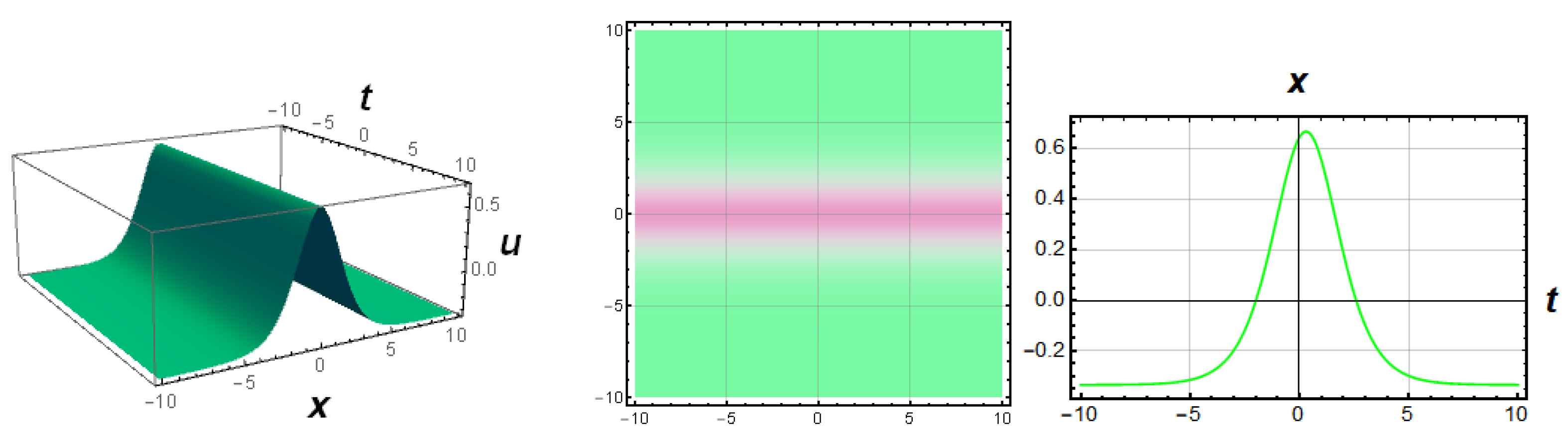
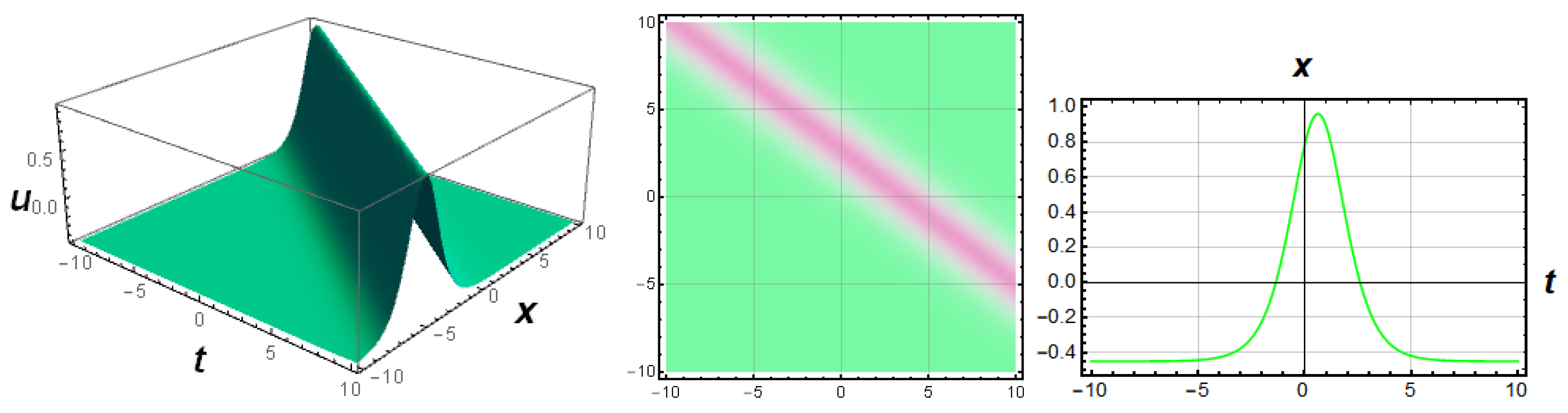
4.5. Results and Discussion

In this work, we obtained a number of analytic solutions to the gFKdVp Equation (3) by invoking the Lie group method together with Kudryashov’s, $(G^{\prime }/G)$ expansion, and the power series solution methods. In this subsection, we give various graphical representations to demonstrate the physical look of the analytic solutions of the Equation (3). Thus, to view the dynamical behavior of the solutions of Equation (3), we assign different values to the constants in the solutions. For instance, Figure 1 depicts the dynamical behavior of the solution (29) in the 3D, density, and 2D plots. The parameters involved in the 3D plot and density plot are given different values, including, $y=0,\nu =1,\mu =1$, and $\alpha =1$, where the variables t and x range from $-10$ to 10. Hence, for the 2D plot, we choose $t=0.5$ and $y=0.3$, where x ranges from $-10$ to 10.

Moreover, the solution (30) is shown in 3D, density, and 2D plots in Figure 2. The parameters are given different values, including, $C_0=1,y=0,\nu =1.5,\mu =1.9$ and $\alpha =1$, where the variables t and x range from $-10$ to 10 for the 3D plot and density plot. Hence, we choose $t=0.5$ and $y=0.3$, where x ranges from $-10$ to 10 for the 2D plot.

Figure 3 depicts the dynamical behavior of the hyperbolic function solution (35) with 3D and density plots with dissimilar values for the parameters of $y=1$, $\beta =0.02,$$\mu =1,\gamma =2,\nu =0.6,\alpha =0.9,L=1,N=1.8$, where the variables x and t range from $-10$ to 10. For the 2D plot, all the parameters from th e3D and density plots remain the same, except for t, in this case $t=1$.

Figure 4 shows the physical look of the rational function solution (37) and the parameters $\mu =0.0001,\gamma =5.009,\nu =0.2,\alpha =0.001,L=1,N=1.8$, with $y=1,$ and x and t ranging from $-200$ to 200. For the 2D plot, these parameters remain the same as for 3D and density plots, except for t, which in this case is $t=1$.

It should be noted from the above results and discussions that by employing different methods to find solutions to the gFKdVp Equation (3), one can obtain solutions of different types that have different physical meanings.

5. Concluding Remarks

To summarize, we used Lie group analysis as well as various other methodologies, including Kudryashov’s method, the $(G^{\prime }/G)$ expansion method, and the power series expansion method, to find analytic solutions to the gFKdVp Equation (3). The solutions were obtained in the form of exponential, trigonometric, hyperbolic, and rational functions. These obtained solutions can be of interest to physicists who are working in this area of research. To demonstrate the dynamical behavior of the obtained solutions, a graphical depiction of the solutions for certain parameter values were also given. The novel solutions developed in this paper may have a substantial influence on future research. At the end, we constructed the conservation law, which provides insight into conserved physical quantities such as energy and momentum, among others, by employing the general multiplier technique and Ibragimov’s method. In future work, one can use the conservation laws obtained here to construct more analytic solutions to the gFKdVp Equation (3).

References

1. Chen, X.; Jüngel, A.; Wang, L. The Shigesada-Kawasaki-Teramoto cross-diffusion system beyond detailed balance. J. Differ. Equ. 2023, 360, 260–286. [Google Scholar] [CrossRef]
2. Khalique, C.M.; Plaatjie, K. Exact solutions and conserved vectors of the two-dimensional generalized shallow water wave equation. Mathematics 2021, 9, 1439. [Google Scholar] [CrossRef]
3. Wazwaz, A.M. Multiple soliton solutions and other scientific solutions for a new Painlevé integrable fifth-order equation. Chaos. Solitons Fractals 2025, 196, 116307. [Google Scholar] [CrossRef]
4. Li, S.; Li, L. Painlevé integrability, auto-Bäcklund transformation and exact solutions of an extended (3+1)-dimensional Boussinesq equation. Qual. Theory Dyn. Syst. 2025, 24, 110. [Google Scholar] [CrossRef]
5. Ovsiannikov, L.V. Group Analysis of Differential Equations; Academic Press: New York, NY, USA, 1982. [Google Scholar]
6. Olver, P.J. Applications of Lie Groups to Differential Equations, 2nd ed.; Springer: Berlin, Germany, 1993. [Google Scholar]
7. Hirota, R. The Direct Method in Soliton Theory; Cambridge University Press: Cambridge, UK, 2004. [Google Scholar]
8. Salas, A.H.; Gomez, C.A. Application of the Cole-Hopf transformation for finding exact solutions to several forms of the seventh-order KdV equation. Math. Probl. Eng. 2010, 2010, 194329. [Google Scholar] [CrossRef]
9. Kudryashov, N.A.; Loguinova, N.B. Extended simplest equation method for nonlinear differential equations. Appl. Math. Comput. 2008, 205, 396–402. [Google Scholar] [CrossRef]
10. Saheli, A.E.; Zogheib, B. Symmetry Analysis of the 3D Boundary-Layer Flow of a Non-Newtonian Fluid. AppliedMath 2024, 4, 1588–1599. [Google Scholar] [CrossRef]
11. Yadav, S. QPDE: Quantum Neural Network Based Stabilization Parameter Prediction for Numerical Solvers for Partial Differential Equations. AppliedMath 2023, 3, 552–562. [Google Scholar] [CrossRef]
12. Monyayi, V.T.; Goufo, E.F.D.; Toudjeu, I.T. Mathematical Analysis of a Navier–Stokes Model with a Mittag–Leffler Kernel. AppliedMath 2024, 4, 1230–1244. [Google Scholar] [CrossRef]
13. Sekhesa, T.M.; Nchejane, N.J.; Poka, W.D.; Kalebe, K.M. Exact solutions of the (1+1)-dissipative Westervelt equation using an optimal system of Lie sub-algebras and modified simple equation method. Partial Differ. Equ. Appl. Math. 2025, 14, 101178. [Google Scholar] [CrossRef]
14. Chatziafratis, A.; Fokas, A.S.; Kalimeris, K. The Fokas method for evolution partial differential equations. Partial Differ. Equ. Appl. Math. 2025, 14, 101144. [Google Scholar] [CrossRef]
15. Ahmed, D.M.; Mahmood, B.A.; Alalyani, A. On the solution of the coupled Whitham–Broer–Kaup problem using a hybrid technique for improved accuracy. Partial Differ. Equ. Appl. Math. 2025, 14, 101184. [Google Scholar] [CrossRef]
16. Darvishi, M.T.; Najafi, M. A modification of extended homoclinic test approach to solve the (3+1)-dimensional potential-YTSF equation. Chin. Phys. Lett. 2011, 28, 040202. [Google Scholar] [CrossRef]
17. Chen, Y.; Yan, Z. New exact solutions of (2+1)-dimensional Gardner equation via the new sine-Gordon equation expansion method. Chaos Solitons Fract. 2005, 26, 399–406. [Google Scholar] [CrossRef]
18. Wang, M.; Li, X.; Zhang, J. The (G/G)-Expansion method and travelling wave solutions for linear evolution equations in mathematical physics. Phys. Lett. A 2005, 24, 1257–1268. [Google Scholar]
19. Feng, L.; Tian, S.; Zhang, T.; Zhou, J. Lie symmetries, conservation laws and analytical solutions for two-component integrable equations. Chin. J. Phys. 2017, 55, 996–1010. [Google Scholar] [CrossRef]
20. Weiss, J.; Tabor, M.; Carnevale, G. The Painlevé property and a partial differential equations with an essential singularity. Phys. Lett. A 1985, 109, 205–208. [Google Scholar] [CrossRef]
21. Wazwaz, A.M. Traveling wave solution to (2+1)-dimensional nonlinear evolution equations. J. Nat. Sci. Math. 2007, 1, 1–13. [Google Scholar]
22. Zheng, C.L.; Fang, J.P. New exact solutions and fractional patterns of generalized Broer-Kaup system via a mapping approach. Chaos Solitons Fractals 2006, 27, 1321–1327. [Google Scholar] [CrossRef]
23. Chun, C.; Sakthivel, R. Homotopy perturbation technique for solving two point boundary value problems-comparison with other methods. Comput. Phys. Commun. 2010, 181, 1021–1024. [Google Scholar] [CrossRef]
24. Zeng, X.; Wang, D.S. A generalized extended rational expansion method and its application to (1+1)-dimensional dispersive long wave equation. Appl. Math. Comput. 2009, 212, 296–304. [Google Scholar] [CrossRef]
25. Kudryashov, N.A. One method for finding exact solutions of nonlinear differential equations, Commun. Nonlinear Sci. Numer. Simulat. 2012, 17, 2248–2253. [Google Scholar] [CrossRef]
26. Gu, C.H. Soliton Theory and Its Application; Zhejiang Science and Technology Press: Hangzhou, China, 1990. [Google Scholar]
27. Lü, J.; Bilige, S.; Chaolu, T. The study of lump solution and interaction phenomenon to (2+1)-dimensional generalized fifth-order KdV equation. Nonlinear Dyn. 2018, 91, 1669–1676. [Google Scholar] [CrossRef]
28. Liu, J.G. Lump-type solutions and interaction solutions for the (2+1)-dimensional generalized fifth-order KdV equation. Appl. Math. Lett. 2018, 86, 36–41. [Google Scholar] [CrossRef]
29. Guo, B.; Fang, Y.; Dong, H. On soliton solutions, periodic wave solutions and asymptotic analysis to the nonlinear evolution equations in (2+1) and (3+1) dimensions. Heliyon 2023, 9, e15929. [Google Scholar] [CrossRef]
30. Ibragimov, N.H. Elementary Lie Group Analysis and Ordinary Differential Equations; John Wiley & Sons: Chichester, NY, USA, 1999. [Google Scholar]
31. Ibragimov, N.H. A new conservation theorem. J. Math. Anal. Appl. 2007, 333, 311–328. [Google Scholar] [CrossRef]
32. Wang, M.; Zhou, Y.; Li, Z. Application of a homogeneous balance method to exact solutions of nonlinear equations in mathematical physics. Phys. Lett. A 1996, 216, 67–75. [Google Scholar] [CrossRef]
33. Simbanefayi, I.; Khalique, C.M. An optimal system of group-invariant solutions and conserved quantities of a nonlinear fifth-order integrable equation. Open Phys. 2020, 18, 829–841. [Google Scholar] [CrossRef]
Figure 1. Hyperbolic solution profile of (29) in 3D, density, and 2D.
Appliedmath 05 00096 g001
Figure 2. Profile of hyperbolic solution (30) in 3D, density, and 2D.
Appliedmath 05 00096 g002
Figure 3. Profile of hyperbolic solution (35) in 3D, density, and 2D.
Appliedmath 05 00096 g003
Figure 4. Profile of rational solution (37) in 3D, density, and 2D.
Appliedmath 05 00096 g004
Disclaimer/Publisher’s Note: The statements, opinions and data contained in all publications are solely those of the individual author(s) and contributor(s) and not of MDPI and/or the editor(s). MDPI and/or the editor(s) disclaim responsibility for any injury to people or property resulting from any ideas, methods, instructions or products referred to in the content.