Article

Neural Networks and Markov Categories

by
Sebastian Pardo-Guerra
1,*,
Johnny Jingze Li
1,2,
Kalyan Basu
1,3 and
Gabriel A. Silva
1,2,4
1
Center for Engineered Natural Intelligence, University of California, San Diego, CA 92093, USA
2
Department of Bioengineering, University of California, San Diego, CA 92093, USA
3
Qualtrics LLC, Seattle, WA 98101, USA
4
Department of Neurosciences, University of California, San Diego, CA 92093, USA
*
Author to whom correspondence should be addressed.
AppliedMath 2025, 5(3), 93; https://doi.org/10.3390/appliedmath5030093
Submission received: 30 April 2025 / Revised: 29 June 2025 / Accepted: 14 July 2025 / Published: 18 July 2025

Abstract

We present a formal framework for modeling neural network dynamics using Category Theory, specifically through Markov categories. In this setting, neural states are represented as objects and state transitions as Markov kernels, i.e., morphisms in the category. This categorical perspective offers an algebraic alternative to traditional approaches based on stochastic differential equations, enabling a rigorous and structured approach to studying neural dynamics as a stochastic process with topological insights. By abstracting neural states as submeasurable spaces and transitions as kernels, our framework bridges biological complexity with formal mathematical structure, providing a foundation for analyzing emergent behavior. As part of this approach, we incorporate concepts from Interacting Particle Systems and employ mean-field approximations to construct Markov kernels, which are then used to simulate neural dynamics via the Ising model. Our simulations reveal a shift from unimodal to multimodal transition distributions near critical temperatures, reinforcing the connection between emergent behavior and abrupt changes in system dynamics.

1. Introduction

Understanding the collective behavior of neurons and the resultant dynamics has been a fundamental challenge in neuroscience, which has driven significant research efforts to unravel the complexities of neural interactions and information processing. From a biological perspective, the dynamics of a neural network is triggered by the collective of both chemical and electric interactions between neurons. In the former, the neurotransmitters convert a chemical signal into an electrical one, which then contributes to the neuron’s summation. The latter, although less frequent than chemical ones, transmits information faster to the post-synaptic neuron’s summation. When enough signals reach a post-synaptic neuron, and push the membrane potential to reach a threshold value, it “fires” an electric signal—also known as action potential-that traverse the body neuron’s axon. Based on these principles, there are several models describing neural network dynamics in terms of the membrane potentials. In some of these models, the evolution of the membrane potential is described as a system of stochastic differential equations (see [1,2,3,4]). However, under some considerations, one can deviate from the coupled stochastic differential equations and focus instead on the derived Fokker-Planck equation of the corresponding system. This alternative perspective allows us to characterize the system’s dynamics in terms of the probability density function. Along these lines, the use of Mean-Field approximations [2,5,6] has shown to be a reliable method for approximating the behavior of the density function, providing a more tractable view of the system’s collective behavior.
In this work, motivated by the Mean-Field approximation of neural dynamics, we delved into formalizing this approach from an algebraic perspective using a mathematical theory called Category Theory (CT). Broadly, CT studies mathematical structures, called categories, which are comprised by two key components: a class of objects, and a class of relations (also called morphisms) between these objects, subject to composition. Due to its high-order level of abstraction, CT has found utility outside pure mathematics. Examples include artificial neural networks [7,8], biological networks [9], social networks [10], information theory [11,12], and Quantum Information theory [13]. Here, we consider a particular type of category, known as Markov category, to settle down the foundations on which we describe neural network dynamics. Precisely, Markov categories can be visualized as an abstract representation of probability distributions and random variables. This approach thus presents a fresh perspective on probability and statistics from an algebraic viewpoint.
After settling our formal framework for neural dynamics, we apply concepts from Interacting Particle Systems (IPSs) as a versatile aspect of our model to capture the local interactions and mutual influences of neurons during dynamics. For our computations, we consider a discrete IPS, where states can have just two values depending on if a neuron is activated or not. In this way, our neural network dynamics is realized as an IPS where the space of states—or configurations—is given by all neural activations. With this in mind, we define the instantaneous transition rates between different configurations through a Markov kernel; which corresponds to a morphism of our neural Markov category.
Lastly, we engage in computational investigations to uncover a fundamental principle inherent in any biological neural network dynamic: emergence. Emergence can be thought as the spontaneous appearance of novel structures or behaviors that are not directly reducible to the properties of individual components. To approach this phenomenon, we study the sudden increase in the transition rate between distant states, highlighting one possible mechanistic basis for such behavior. Indeed, when the transition rate across such states undergoes a substantial jump, the system constructively reorganizes its dynamics, potentially giving rise to emergent properties. In order to sustain this hypothesis, we first realize neural network dynamics as an IPS and frame it as an Ising Model.
All together, we verify at the critical points of the Ising model that there exists a substantial increase in the transition rate between different and distant neural states, thus showing a potential emergent behavior.

2. Neural Networks as Markov Categories

Traditionally, models of neural network dynamics are framed using stochastic differential equations. Within these frameworks, the evolution of activity in the network can be modeled as an Ornstein–Uhlenbeck process or described using the Langevin equation, both of which are continuous approximations derived from the Fokker-Planck equation, itself a limiting case of the master equation. These approaches aim to capture the microscopic stochastic fluctuations of the system, modeling its behavior at a lower level of abstraction. In contrast, one can view neural network dynamics through the lens of measure-preserving dynamical systems. This perspective operates at a higher level, emphasizing the global or macroscopic evolution of the system. It is more naturally suited for capturing structural, algebraic, and possibly emergent properties of the network, providing a formal setting in which we can define and study laws that govern the system’s behavior beyond the stochastic microdynamics. Markov categories thus offer a powerful categorical framework that unifies these perspectives. They allow us to model stochastic processes compositionally while also accommodating abstract structural features, making them a natural language for connecting microscopic randomness with emergent macroscopic order in neural systems.
We now introduce our formal framework describing neural network dynamics in terms of a Markov category. Broadly speaking, Markov categories are algebraic structures that describe, in a synthetic way, aspects of probability and statistics. This description provides simple and purely algebraic axioms for systems of Markov kernels, allowing us to study and explore both fields from a high-level perspective. Recall that, in Probability Theory, a Markov kernel is a function that generalizes the notion of transition rate matrix of a Markov process with a finite state space to any measurable space. However, from a Category Theory perspective, Markov kernels can be conceived as morphisms of the Kleisli category associated to the Giry monad defined in the category of measurable spaces and measurable functions. This Giry monad is also called the probability monad over the category of measurable spaces. The first notion of Markov categories can be traced back to Golubtsov’s work in a slightly different approach [14]. Nevertheless, it was not until Fong’s contributions to the categorical structure of Bayesian networks [15] that Markov categories started to be realized as some sort of category that behaves like a category of Markov kernels. These notions reappeared implicitly in subsequent works by Jacobs and Zanasi [16], and their explicit axiomatization was later undertaken by Cho and Jacobs in the context of their categorical exploration of conditional independence and Bayesian inference [17]. There, Cho and Jacobs attributed the term “affine CD-categories”, where “CD” denotes a “Copy/Discard” operation, capturing the essence of the morphisms’ structure. More recently, Fritz [18] detailed precisely Markov categories as abstract generalizations of categories that behave like categories of Markov kernels, thus realizing morphisms as maps that assign to every input value a probability distribution over the output values. Algebraically,
Definition 1 
([18]). A Markov category C is a symmetric monoidal category in which every object X C is equipped with a commutative comonoid structure given by a comultiplication c o p X : X X X and a counit d e l X : X I , depicted in string diagrams as
Appliedmath 05 00093 i001and satisfying the commutative comonoid equations,
Appliedmath 05 00093 i002as well as compatibility with the monoidal structure,
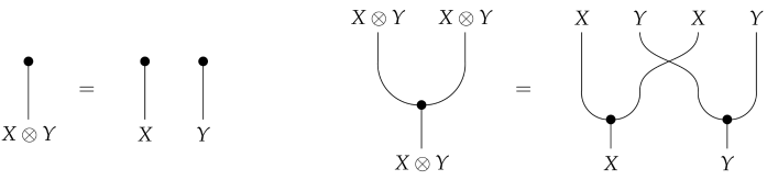
Appliedmath 05 00093 i003and naturality of d e l , which means that
Appliedmath 05 00093 i004for every morphism f.
For instance, we can consider the category FinStoch which has finite sets for objects, and stochastic matrices as morphism. In this case, given a morphism f : X Y between finite sets X and Y, we understand the entry f i , j of the stochastic matrix f = ( f x , y ) x X , y Y as the probability that the Markov kernel f outputs j given the input i. Also, the entries ( f x , y ) x X , y Y are nonnegative real numbers that satisfy y Y f x , y = 1 , for every x X . Another example consists of Stoch which has measurable spaces for objects and measurable Markov kernels as morphisms. Although this category fails in the existence of conditionals, it contains a subcategory—namely BorelStoch—which has Borel spaces as objects and measurable Markov kernels as morphisms, and for which conditionals are well defined [18].

A Neural Network Markov Category

Throughout this section, we will denote a neural network by G and its corresponding vertex set by V ( G ) . Each neural state or activation corresponds to a function η : V ( G ) { 0 , 1 } , where { 0 , 1 } denotes the two possible states at which a neuron can be: 0 if the neuron is inactive and 1 if the neuron is active. The set of all possible activation comprises what we call the neural state space and will be denoted by
X = η η : V ( G ) { 0 , 1 } .
We now provide some basic notions and definitions with which we build our category for a neural network.
Definition 2. 
A topological space is a set X together with a collection of open subsets  τ P ( X ) satisfying the following conditions:
(i
The empty set and X belong to τ.
(ii
The intersection of a finite number of sets in τ is also in τ.
(iii
The union of an arbitrary number of sets in τ is also in τ.
Considering the above definition, the set X of neural states becomes a topological space when we take the power set P ( X ) as the set of open sets. In fact, this topology is called the discrete topology because any subset of X gives rise to an open set. Now, the power set P ( X ) ) also satisfies some closure properties. In fact, P ( X ) is closed under countable unions, countable intersections, and under complements. These three properties constitute what we call a measurable space. Formally,
Definition 3. 
A measurable space is any tuple ( X , Σ X ) where X is a set, and Σ X is a σ-algebra, that is, a collection of subsets of X which is closed under countable unions, countable intersections, and under complement.
Henceforth, we will think of a neural network as both a topological and measurable space ( X , Σ X ) . Here, X corresponds to the neural state space, whereas Σ X corresponds to the σ -algebra generated by the topology on X . Observe that, when considering the discrete topology, we obtain that X coincides with the power set P ( X ) . With this in mind, if we visualized a neural network dynamics as a collection of random variables on the neural state space that behaves like a Markov process, then, the probability density function would be captured by a Markov kernel, which plays a similar role to that of a transition matrix in the theory of Markov processes with a finite state space. Explicitly:
Definition 4. 
A Markov kernel between the measurable spaces  ( X , Σ X ) and ( Y , Σ Y ) is a map κ : Σ Y × X [ 0 , 1 ] with the following properties:
(i
For every B Σ Y , the map x κ ( B , x ) is Σ X -measurable.
(ii
For every x X , the map B κ ( B , x ) defines a probability measure on ( Y , Σ Y ) .
Considering the above, we arrive at our definition of a neural network category:
Definition 5. 
Let G be a neural network and let X be its neural state space. The neural network category, denoted by C a t ( X ) , has as objects all submeasurable spaces ( A , Σ A ) of the measurable space ( X , Σ X ) , and as morphisms Markov kernels between these measurable spaces.
Remark 1. 
In general, the category C a t ( X ) is a subcategory of the broader category Stoch. However, for our applications, we will consider finite neural networks, thereby all sets of our neural states are finite. Thus, our neural network category will be actually a subcategory of FinStoch.
Remark 2. 
Under the above definition, each dynamics on a neural network is conceived as a functor from a monoid category with one object to our neural network category.

3. Modeling the Neural Network Markov Category

In this section, we delineate the construction of our morphisms -or Markov kernels- which we use to approximate a neural network dynamics. To that end, we will conceive that neural network dynamics behaves as an Integrating Particle System, and use Mean-Field approximation to compute its Hamiltonian.
To put in context our construction, we first provide a brief introduction of some Mean-Field approximations in the field of neuroscience. In [2], Fasoli and Vedadi describe neural network dynamics as a system of stochastic differential equations. Each equation represents the membrane potential evolution of a neuron V i of the network, and has the form
d V i ( t ) = 1 τ V i ( t ) + j = 0 N 1 J i j S ( V j ( t ) ) + I ( t ) d t + σ d B i V ( t ) .
Here, V i ( t ) is the membrane potential of the i-th neuron, N denotes the number of neurons of the system, τ is a time constant that describe the speed of convergence to a stationary state, I ( t ) is the deterministic external input current, B i V ( t ) describes the background noise of neuron v i , S is a function that converts the membrane potential of a neuron into the rate of frequency of spikes it generates, and σ is the standard deviation of the Brownian motion. In order to apply a mean-field approximation, the authors assumed the thermodynamic limit condition: this means that the number of neurons in the system grows to infinity. In this case, there is an emergent phenomenon known as propagation to chaos that elucidates the fact that the number of independent neurons increases as the network grows in size. With this in mind, when the number of incoming signals for each neuron grows to infinity, in the thermodynamic limit the set of neurons becomes independent, and thus, they share the same marginal probability density. As a result, the set of all neurons V i can be conceived as a collection of samples generated by a single probability distribution p ( V , t ) . In this process, the thermodynamic limit condition is helpful in obtaining a decoupled set of equations, with which the probability density function of the ensemble can be expressed as the product of marginal probability densities
p ( V 0 , , V n 1 , t ) = Π i = 0 n 1 p ( V i , t ) .
Another approach has been used by Friston, Sajid and Parr in [6]. There, they considered the variational free energy, based on the Bogolyubov inequality [19], to approximate the Hamiltonian of the whole system. In this case, the Hamiltonian is approximated by minimizing the Helmholtz free energy. Precisely, they start by assuming that the probability of the system has the form
p ( x ) = 1 Z e β H ( x ) ,
where H denotes the Hamiltonian, and Z represents the partition function
Z = e β H ( t ) d t ,
also known as the normalizing constant. This partition function, in fact, is closely related to the Helmholtz free energy, used to approximate the system energy. Thus, by replacing the conditional probability with a variational density q, the Bogolyugov inequality implies that the Helmholtz free energy of an interacting system is always less than the free energy using the original Hamiltonian. In this way, the variational free energy F q is an upper bound on the Helmholtz free energy F. Consequently, by minimizing the former, one gets a good approximation of the latter.
Considering the above, one can get a factorization of the system into a series of marginal distributions as a consequence of the decomposition of the Hamiltonian in terms of the variational densities
q ( x ) = Π i q ( x i ) ,
where q ( x ) = e β h ( x i ) Z i , and H q = i h i ( x ) . This factorization is essentially their mean-field approximation.
In this work, we will proceed in a similar direction to the last approach, this is, we first frame our system as an IPS and then compute the Hamiltonian using a mean-field approximation.

Interacting Particle System Approach

We start by framing neural network dynamics as an stochastic process that behaves as an IPS. This relies on the principle that brain dynamics emerges from stochastic interactions among individual components that collectively determine the behavior of the whole system. Broadly speaking, an IPS is a stochastic process that involves a collection of random variables, each of which represents the state of an individual particle, agent, or component within the system. The evolution of the system is then governed by interaction rules that specify how the particles influence each other. These rules are often expressed as conditional probabilities, indicating the probability of a particle transitioning from one state to another based on the states of its neighbors. For the purpose of this work, we will consider that spins are discrete values taken in { 0 , 1 } .
From an IPS context, given a neural network G, the site space of the stochastic process is the set of vertices V ( G ) , the state space representing all possible states is the discrete set S = { 0 , 1 } , and the configuration space is given by the set of all functions describing neural states (or activations), that is,
X = { η η : V ( G ) { 0 , 1 } } = S G .
Remark 3. 
In order to view our neural network as an IPS, we will assume that our neural network V ( G ) is contained in an infinite countable graph G ˜ . Nonetheless, we will think that the activation space is realized only upon V ( G ) .
The Hamiltonian for our IPS has the form:
H ( η ) = j i H [ j ] J i , j η ( i ) η ( j ) j h j η ( j ) .
Here, H [ j ] represents the upstreaming nodes to node j, J i , j the coupling strength of the connection going from neuron i towards neuron j, and h j is an external field interaction associated to each neuron j. Now, as each edge ( i , j ) occurs only once in H [ j ] , the above sum takes the form
H ( η ) = i , j J i , j η ( i ) η ( j ) j h j η ( j ) .
The above equation can be seen as an inhomogeneous or disordered Ising model. Nevertheless, by fixing the variable J i , j as part of the signs, we can then treat it as a non-correlated factor that is independent to η ( i ) and η ( j ) . In fact, this will be reflected as the expected value for J i , j in the final analysis, which allowing us to set it as the mean of the weight distribution. In this way, the Ising model now becomes homogeneous, and thus, we can follow the approach described by Sakthivadivel in [20]. Indeed, by considering the Hamiltonian in (1), one starts with the trial Hamiltonian
H ^ 0 = j m i η ( j ) ,
to then obtain the equation
m = J i , j s j 0 + h ,
which in turn leads us to describe the mean field value as
m = J i , j tanh ( β m ) + h .
Here, the sum is taken over neighboring spins. The above equation reflects the sum of neighboring spins that persists from our original Hamiltonian. However, due to the effective field, we can reduce the equation to multiplication by the number of neighbors z. Therefore, the final mean-field value is
m = z J tanh ( β m ) + h .
With this mean-field approximation in mind, we compute the Hamiltonian H of the system and use it to define the transition rates from one neural state (or configuration) to another. To that end, we consider Glauber dynamics to simulate the IPS concerning our neural network dynamics, equipped with the next transition probabilities (see [21]):
p Λ ( η | ξ ) = 1 + tanh β Δ H 2 n if ξ B ( η ) , 1 x B ( ) 1 + tanh β Δ H 2 n if ξ = η , 0 otherwise .
In the above expression, Λ is a subset of the site space V ( G ) , B ( η ) denotes the set of configurations that differ from η in exactly one spine and whose site lies in the set Λ , and lastly, Δ H = H ( η ) H ( ξ ) . It can be shown [22] that these transition rates, along with the procedures they arise from, give rise to a unique stationary distribution corresponding to the standard Boltzmann-Gibbs distribution given by
P ( η ) = e β H ( η ) Z ,
with Z = η e β H ( η ) .
Remark 4. 
At this point, we are assuming that neural dynamics behaves as a stochastic jump process, that is, a process whose transitions between discrete states spend an amount of time -called the holding time-in each current state before jumping to the next state, where again it spends another holding time. With this in mind, we can realize neural dynamics as a Markov jump process whose holding times are exponentially distributed.
Grounded on the transition probabilities in (3), we define the Markov kernel conditions as follows: if η X and B Σ Y , then,
κ ( B , η ) = max { p ( η | ξ ) ξ B } ,
where Λ = V ( G ) and p ( η | ξ ) denotes the transition probability from state η to state ξ .
It is worth mentioning that, for the computations we present in the following section, all Markov kernels correspond to a transition rate matrix given by the Markov process and its node’s updates. These Markov kernels, in turn, amount to morphisms of our neural network Markov category. Consequently, as noted in Remark 1, our neural network Markov category lies within the category FinStoch.

4. Emergence in Neural Networks Dynamics

In this section, we discuss the notion of emergence in neural dynamics by applying our framework to the evolution of a dynamical system that leads to, potentially, a phase transition in the system. To that end, we start recalling the mathematical formulation of generative effects or emergence of a system described by Adams in [23]. Let us assume we have a system S described by the category C ; that is, the objects of C correspond to the elements of the system S, while the morphisms in C represent the relations between elements in S. Then, a transformation (or in Adams’ context a veil ) on the system S is a functor from the category C to itself. Following Adams theory, one says that a transformation sustains generative effects if the property of exactness is lost, this is, if the functor does not preserve exact sequences. In particular, for a system whose representation as a category has the form of a lattice (A lattice is a partially ordered set in which any two elements have a least upper bound, denoted by ∨, and a greatest lower bound denoted by ∧.), the definition of emergence takes a simpler format. In this case, one says that a transformation φ sustains generative effects if
φ ( x x ) φ ( x ) φ ( x ) .
Considering the above, if we think of a system as the neural state space X for a neural network dynamics, then the measurable space ( X , X ) can be ordered by inclusion, and thus, it gives rise to a lattice whose elements correspond to submeasurable spaces and whose meet and join operations are given by the intersection ∩ and the union ∪ of sets, respectively. Within this context, the condition φ ( x x ) φ ( x ) φ ( x ) concerns the breaking in the topology with respect to the σ -algebra of X .
Building on our framework, we investigate emergent phenomena through Markov kernels and the transition probabilities defined for our neural state space. From a lattice-structure perspective, an emergent behavior should occur when the system transitions to a state that is significantly distant from the current state with a high probability, as such transition is likely to give rise to the inequality above. Indeed, the probability of a system transitioning from one state to another is generally high when the states are similar, indicating that they are ’close’ in the system’s state space. This closeness ensures that the transition maintains a level of continuity, preserving the system’s underlying topological structure. In such cases, small changes in state reflect gradual, predictable dynamics. However, as we explore below, the dynamics shift dramatically when emergent states come into play—particularly during phenomena like phase transitions. In these scenarios, the system can make a sudden leap between states that are topologically distant from each other, yet this transition occurs with a surprisingly high probability. Such emergent behavior signifies a break from gradual change, reflecting a fundamental shift in the system’s organization. These high-probability jumps between distant states suggest the presence of new, dominant interactions or structures within the system, revealing deeper layers of complexity in its dynamics.
More precisely, when a measure is defined on the neural state space, the resulting probability distribution tends to follow a normal (Gaussian) distribution. This means that the system is more likely to transition to states that are nearby, instead of transitioning to states that are farther away, since these occur with lower probability. Nevertheless, when an emergent behavior occurs—for instance, a phase transition—the state of the network goes through a drastic change, which is then conceptualized as a major shift in the neural state space. Within this line, we expect to observe the next behavior: right before a phase transition occurs, the probability of having this major shift in the state space is higher, and thus resulting in a distribution that does not follow a normal distribution anymore. To detect this big change in the neural network states (phase transition, bifurcation, etc.), we focus on the shift in the shape of the probability distribution, which is, essentially, reflected by the energy level of the system.

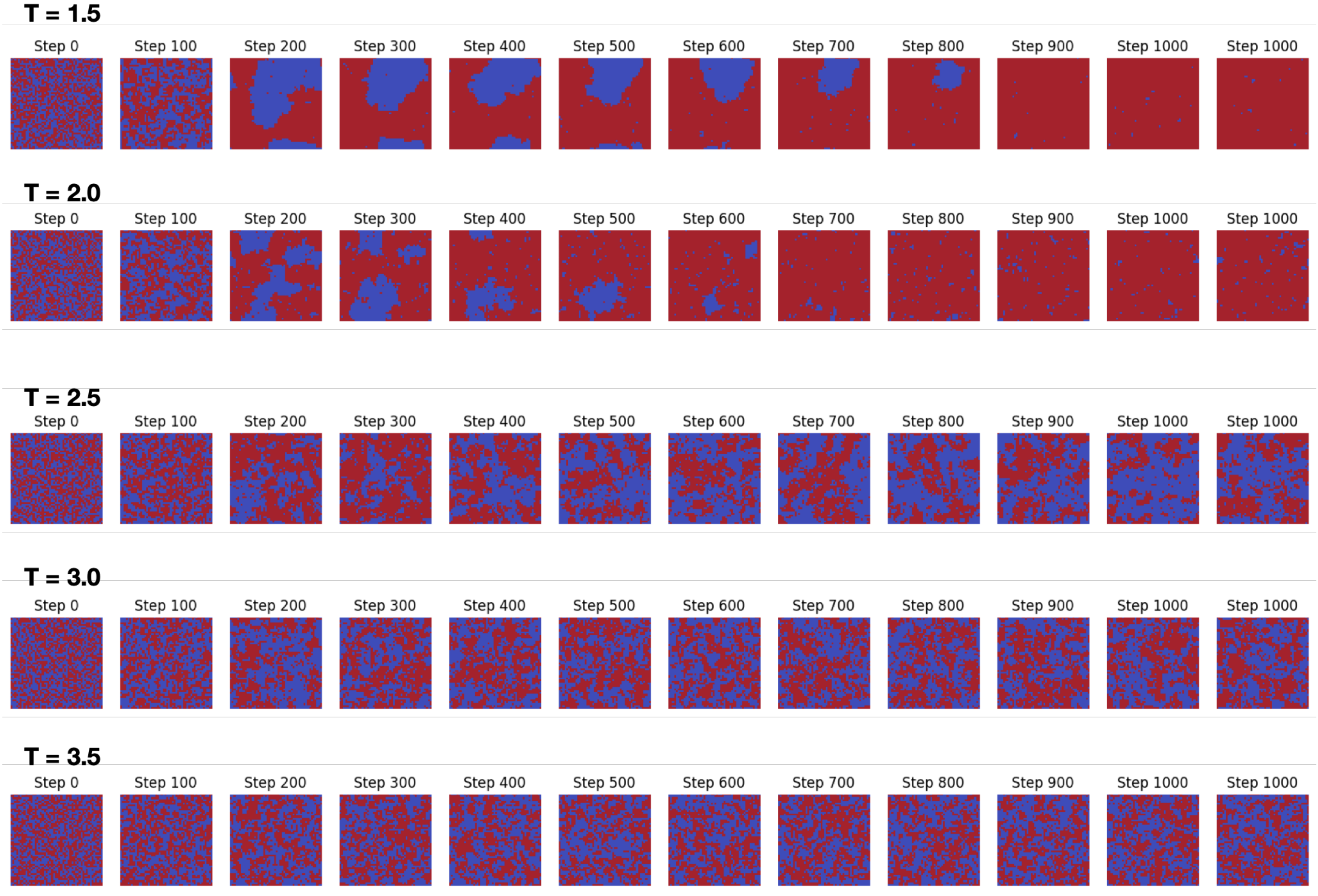
Numerical Computations

For our numerical computations, we begin by modeling a neural network as an IPS, using the Ising model as a reference. This choice is motivated by two main reasons. First, the Ising model is one of the most well-studied IPS frameworks in multiple dimensions and serves as a canonical example of systems exhibiting critical phenomena, such as phase transitions, with a rich and well-understood mathematical structure. Second, as an IPS, the Ising model naturally captures the notion of locally constrained dynamics, where the system’s evolution depends only on the state of neighboring sites in the underlying graph. This locality is a distinctive feature of IPS models and is absent from global probabilistic models like differential equations, which typically lack an intrinsic notion of local interaction rules.
However, a key limitation of the standard Ising model in the context of neural dynamics is its assumption of a fixed coupling constant. This simplification may fail to capture the heterogeneous and adaptive nature of real neural systems. While we adopt the Ising model in this work for simplicity, the framework can be naturally extended to a Spin Glass model, in which the coupling constants are drawn from a probability distribution. This generalization accommodates greater dynamical complexity and offers a more realistic representation of neural phenomena, such as spike-timing-dependent plasticity.
Our simulation builds upon the Hamiltonian of an Ising model with the coupling constant J = 1 . The critical temperature is achieved at T C = 2.269 , and the transitional probability—based on the Glauber dynamics—is defined as
p ( Δ E ) = 1 , Δ E 0 e Δ E / T , Δ E > 0 .
We observe that as the temperature approaches its critical value, the transition probability distribution undergoes a significant transformation in its shape. Specifically, it shifts from a unimodal distribution to a multimodal one, leading to the emergence of additional local maxima. This structural change creates the potential for emergent behaviors (Figure 1).
In Figure 2, we see that when T < T C , the system converges to an ordered phase, while for T > T C the system converge to a disordered phase. In particular, as some studies like [24,25] show, when the temperature of the Ising model is closer to the critical number T C , the systems tend to show a stronger dynamical variety, with more intricate patterns of activations in the state space. Thus, this reinforces the idea that an emergent behavior occurs when the system goes through a major shift in the state space.
We quantitatively study the diversity of the dynamics under different temperatures, which as we argued, reflects the level of emergence of the system. Figure 3 displays the ensemble–averaged transition–probability density obtained from 50 statistically independent hot–start realizations of the two–dimensional Glauber–Ising model. (Simulation parameters: lattice size L = 48 , full-lattice sweeps per run of 10 5 steps, the first 1 × 10 4 sweeps discarded as burn-in. At every sweep we record the Boltzmann acceptance probability p ( Δ E ) for each attempted flip and build a sweep-level probability–mass function; these PMFs are then averaged over the 50 runs). The horizontal axis reports the total magnetization of the state the system could be transitioning to, so we can evaluate the metric “distance’’ between the two micro-states, while the vertical axis shows the corresponding probability mass. Three qualitative regimes emerge:
1.
Deep sub-critical ( T T c ). The density is sharply local: the system either stays in the same state ( Δ E = 0 ) or makes a near-neighbor move ( | Δ E | = 4 J ). Long-range jumps are practically forbidden, reflecting a single-basin energy landscape.
2.
Near-critical ( T T c ). The distribution broadens and develops broad shoulders at | Δ E | { 4 J , 8 J } . As the curve in the figure is averaged over 50 runs, this spread quantifies genuine dynamical diversity as follows: different realizations explore macroscopically distinct pathways with comparable weight. The increased width signals a higher degree of emergence, as the system spends non-negligible probability mass in multiple, topologically distant regions of state space.
3.
Super-critical regime ( T T c ). In contrast to the broad, multi-modal curve observed at criticality, the transition-probability density collapses into a sharp peak centered at Δ E = 0 . At high temperature each spin flips almost independently; the energy increments of the L 2 trial moves add up to a sum of weakly correlated random variables. By the central limit theorem the distribution of these sums (and therefore of the sweep–level transition probabilities) becomes Gaussian with variance σ 2 L 2 , i.e. vanishingly small for macroscopic lattices. Physically, the system no longer supports large, coherent domains, so any individual flip typically changes the energy by only a single-bond amount and the net change over a sweep is close to zero with overwhelming probability. The disappearance of side lobes therefore signals the loss of emergent structure in the high-temperature phase.
Taken together, this result corroborates our theoretical claim that emergence can be operationalized by the shape of the transition-probability distribution. Close to the critical point the system maximizes this breadth, hence maximizes its emergent potential. A practical consequence is that one can classify emergent behavior by computing graph-theoretic descriptors (e.g., entropy, algebraic connectivity) of the network obtained by linking states whose mutual transition probabilities exceed a chosen threshold; the wider and more clustered the distribution, the richer the resulting network and the stronger the emergence.

5. Conclusions

In this work, we claim that emergent behavior within neural dynamics can be characterized by significant transitions between states that are markedly distinct or are distant from one another. This perspective provides a novel lens for understanding how complex behaviors arise in neural systems and aligns with broader theoretical frameworks in dynamical systems, network theory, and machine learning.
Our proposal builds on prior work that defined potential emergence in terms of the number of paths connecting regions of a network. While this earlier framework focused on the combinatorial richness of the network’s connections, the current perspective emphasizes on the dynamical rates at which transitions occur. Although our framework provides a useful theoretical foundation, several challenges remain. First, quantifying “distance” between states in a way that is both general and context-specific requires further exploration. Additionally, understanding the mechanisms that trigger large jumps in transition rates—whether due to external stimuli, intrinsic network properties, or stochastic fluctuations—is crucial for making predictive models of emergent behavior.
A promising direction for future research is to extend the present model to a Spin Glass framework, in which the coupling constants are drawn from a probability distribution. This extension could provide a more faithful representation of real neural dynamics, particularly in capturing adaptive processes such as spike-timing-dependent plasticity. Another potential avenue involves the application of more advanced analytical tools, such as renormalization group theory, which may offer deeper insights than traditional mean-field approximations, especially in regimes where fluctuations and correlations play a crucial role. Additionally, one can explore richer local structures in the space of neural states by incorporating higher-order interactions through simplicial complexes. Unlike standard pairwise synaptic models, which represent relationships between individual pre-and post-synaptic neurons, simplicial complexes allow for the modeling of collective interactions among groups of neurons. This could reflect the fact that spike-timing-dependent plasticity may induce coordinated changes across multiple, non-directly connected neurons that fire together, thereby capturing the emergence of high-order dependencies in the network.

Author Contributions

Conceptualization, S.P.-G., J.J.L., K.B. and G.A.S.; Methodology, S.P.-G. and K.B.; Software, J.J.L.; Validation, S.P.-G., J.J.L., K.B. and G.A.S.; Formal analysis, S.P.-G., J.J.L. and K.B.; Investigation, S.P.-G., J.J.L. and K.B.; Data curation, J.J.L.; Writing—original draft, S.P.-G.; Writing—review and editing, S.P.-G. and J.J.L.; Visualization, S.P.-G.; Supervision, K.B. and G.A.S.; Project administration, G.A.S. All authors have read and agreed to the published version of the manuscript.

Funding

This research received no external funding.

Data Availability Statement

Data are contained within the article.

Acknowledgments

The authors thank the referees for their careful reading and accurate comments.

Conflicts of Interest

Author Kalyan Basu was employed by the company “Qualtrics LLC”. The remaining authors declare that the research was conducted in the absence of any commercial or financial relationships that could be construed as a potential conflict of interest.

References

  1. Bossy, M.; Fontbona, J.; Olivero, H. Synchronization of stochastic mean field networks of Hodgkin–Huxley neurons with noisy channels. J. Math. Biol. 2019, 78, 1771–1820. [Google Scholar] [CrossRef] [PubMed]
  2. Fasoli, D. Attacking the Brain with Neuroscience: Mean-Field Theory, Finite Size Effects and Encoding Capability of Stochastic Neural Networks. Ph.D. Thesis, Université Nice Sophia Antipolis, Nice, France, 2013. [Google Scholar]
  3. Philippe, R.; Vignoud, G. Stochastic models of neural synaptic plasticity. SIAM J. Appl. Math. 2021, 81, 1821–1846. [Google Scholar] [CrossRef] [PubMed]
  4. Sacerdote, L.; Giraudo, M.T. Stochastic Integrate and Fire Models: A review on mathematical methods and their applications. In Stochastic Biomathematical Models: With Applications to Neuronal Modeling; Springer: Berlin/Heidelberg, Germany, 2013; pp. 99–148. [Google Scholar]
  5. Faugeras, O.; Touboul, J.; Cessac, B. A constructive mean-field analysis of multi-population neural networks with random synaptic weights and stochastic inputs. Front. Comput. Neurosci. 2009, 3. [Google Scholar] [CrossRef] [PubMed]
  6. Parr, T.; Sajid, N.; Friston, K.J. Modules or Mean-Fields? Entropy 2020, 22, 552. [Google Scholar] [CrossRef] [PubMed]
  7. Fong, B.; Spivak, D.; Tuyéras, R. Backprop as Functor: A compositional perspective on supervised learning. In Proceedings of the 34th Annual ACM/IEEE Symposium on Logic in Computer Science (LICS), Vancouver, BC, Canada, 24–27 June 2019; pp. 1–13. [Google Scholar] [CrossRef]
  8. Li, J.J.; Prado-Guerra, S.; Basu, K.; Silva, G. A Categorical Framework for Quantifying Emergent Effects in Network Topology. arXiv 2024, arXiv:2311.17403. [Google Scholar]
  9. Haruna, T. Theory of interface: Category theory, directed networks and evolution of biological networks. Biosystems 2013, 114, 125–148. [Google Scholar] [CrossRef] [PubMed]
  10. Otter, N.; Porter, M.A. A unified framework for equivalences in social networks. arXiv 2020, arXiv:2006.10733. [Google Scholar]
  11. Northoff, G.; Tsuchiya, N.; Saigo, H. Mathematics and the Brain: A Category Theoretical Approach to Go Beyond the Neural Correlates of Consciousness. Entropy 2019, 21, 1234. [Google Scholar] [CrossRef]
  12. Pardo-Guerra, S.; Silva, G. Preradical, entropy and the flow of information. Int. J. Gen. Syst. 2024, 53, 1121–1145. [Google Scholar] [CrossRef]
  13. Parzygnat, A.J. Inverses, disintegrations, and Bayesian inversion in quantum Markov categories. arXiv 2020, arXiv:2001.08375. [Google Scholar]
  14. Golubtsov, P.V. Monoidal Kleisli category as a background for information transformers theory. Inf. Theory Inf. Process. 2002, 2, 62–84. [Google Scholar]
  15. Fong, B. Causal Theories: A Categorical Perspective on Bayesian Networks. arXiv 2013, arXiv:1301.6201. [Google Scholar]
  16. Jacobs, B.; Zanasi, F. A Predicate/State Transformer Semantics for Bayesian Learning. Electron. Theor. Comput. Sci. 2016, 325, 185–200. [Google Scholar] [CrossRef]
  17. Cho, K.; Jacobs, B. Disintegration and Bayesian inversion via string diagrams. Math. Struct. Comput. Sci. 2019, 29, 938–971. [Google Scholar] [CrossRef]
  18. Fritz, T. A synthetic approach to Markov kernels, conditional independence and theorems on sufficient statistics. Adv. Math. 2020, 370, 107239. [Google Scholar] [CrossRef]
  19. Bogolyubov, N.N. On model dynamical systems in statistical mechanics. Physica 1966, 32, 933–994. [Google Scholar] [CrossRef]
  20. Sakthivadivel, D. Magnetisation and mean field theory in the Ising model. SciPost Phys. Lect. Notes 2022, 35. [Google Scholar] [CrossRef]
  21. Rosas, F.E.; Geiger, B.C.; Luppi, A.I.; Seth, A.K.; Polani, D.; Gastpar, M.; Mediano, P.A. Software in the natural world: A computational approach to hierarchical emergence. arXiv 2024, arXiv:2402.09090. [Google Scholar]
  22. Glauber, R.J. Time-Dependent Statistics of the Ising Model. J. Math. Phys. 1963, 4, 294–307. [Google Scholar] [CrossRef]
  23. Adam, E.M. Systems, Generativity and Interactional Effects. Ph.D. Thesis, Department of Electrical Engineering and Computer Science, Massachusetts Institute of Technology, Cambridge, MA, USA, 2017. [Google Scholar]
  24. Morales, I.; Landa, E.; Angeles, C.; Toledo, J.; Rivera, A.; Temis, J.; Frank, A. Behavior of early warnings near the critical temperature in the two-dimensional Ising model. PLoS ONE 2015, 10, e0130751. [Google Scholar] [CrossRef] [PubMed]
  25. Morningstar, A.; Melko, R. Deep learning the ising model near criticality. J. Mach. Learn. Res. 2018, 18, 1–17. [Google Scholar]
Figure 1. Transition Probability distribution at different temperatures.
Appliedmath 05 00093 g001
Figure 2. Simulation of 2D Ising model at different temperatures.
Appliedmath 05 00093 g002
Figure 3. Transition-probability distributions Pr ( Δ E ) for a 48 × 48 Ising lattice (Glauber dynamics) at five temperatures. Each curve is averaged over a 5-step window to smooth stochastic fluctuations.
Appliedmath 05 00093 g003
Disclaimer/Publisher’s Note: The statements, opinions and data contained in all publications are solely those of the individual author(s) and contributor(s) and not of MDPI and/or the editor(s). MDPI and/or the editor(s) disclaim responsibility for any injury to people or property resulting from any ideas, methods, instructions or products referred to in the content.

