Abstract
As cities grow denser, the demand for efficient parking systems becomes more critical to reduce traffic congestion, fuel consumption, and environmental impact. This paper proposes a smart parking solution that combines deep learning and algorithmic sorting to identify the nearest available parking slot in real time. The system uses several pre-trained convolutional neural network (CNN) models—VGG16, ResNet50, Xception, LeNet, AlexNet, and MobileNet—along with a lightweight custom CNN architecture, all trained on a custom parking dataset. These models are integrated into a mobile application that allows users to view and request nearby parking spaces. A merge sort algorithm ranks available slots based on proximity to the user. The system is validated using benchmark datasets (CNR-EXT and PKLot), demonstrating high accuracy across diverse weather conditions. The proposed system shows how applied mathematical models and deep learning can improve urban mobility through intelligent infrastructure.
1. Introduction
Recently, there has been enough development of technologies. The Internet of Things (IoT) is a famous technology in the modern era and is in increasing demand. The IoT is used to remotely control objects, and its structure typically consists of three elementary layers. The first is the sensing layer, and it contains visual or scalar sensors that receive data in real time from its surroundings. The second is the network layer, and it is the one responsible for transporting and routing the data between different systems, typically employing protocols such as IP and ICMP. The third is the application layer, where software processes the compiled data and facilitates real-time communication with devices. Of all the various IoT applications, we view smart parking systems as crucial components of a smart city that provide real-time information on available and used parking spaces. This technology has simplified daily living compared to 10 years ago. With so many additional automobiles entering the road every day, parking issues have come to the forefront of public discussion in recent years [1,2].
One of the most fundamental and essential requirements for smart cities is smart parking systems. A driver looking for a parking space wastes 17 h a year on intermediates. This has caused the smart parking sector’s rapid growth and the frequent introduction of fresh ideas.
Multiple current procedures employ sensors at each location to decide whether parking spaces are available. A straightforward solution to the issue of automated parking place recognition has been to set up sensors in each parking space. Nevertheless, the equipment and implementation costs are quite high, particularly for certain large and historic buildings. One of the more significant issues is that there is not a lot of detailed sensor information available; whether a parking space is occupied or not is typically known, but other information, such as the license plate number or vehicle type (car or motorbike), is not available. To help fix this, some advanced systems use cameras as sensors in every parking space to gather more detailed data. This provides space for numerous other clever features, such as the ability to allow the user to locate their car via its license plate number. However, this type of technology needs a strong network throughout the parking area. A network infrastructure faces several difficulties due to the massive bandwidth requirements for gathering camera data. Another option by which to address parking issues is through using autonomous cars [3]. However, one disadvantage [4] of this is that passengers will disembark from the vehicle at the location and then go off to locate a parking space by themselves. In this situation, an automobile could circle the surrounding area, searching for a parking spot, and obstruct others and waste petrol. Another option for solving this issue is to use robotic valet methods [5], although doing so would require costly and sophisticated mechanical apparatus. By using vision-based algorithms to cover large parking zones, specific systems lower the cost of sensor installation [6,7]. A deep learning approach solution built using the VGGNet group has been implemented to solve the parking space detection problem.
In recent years, computer vision-based smart parking systems have garnered substantial attention, driven by advancements in deep learning and the growing need for scalable, real-time solutions deployable on edge devices. These systems leverage camera feeds and deep neural networks to monitor and manage parking areas efficiently, often reducing the need for costly ground sensors [7]. For instance, a deep learning solution based on the VGGNet group was implemented to detect parking space occupancy, demonstrating the effectiveness of convolutional models in structured parking scenarios. In [8], a hybrid approach utilizing Faster R-CNN and YOLOv3 enabled the real-time detection of available slots, significantly improving urban traffic flow by notifying drivers about free parking spaces through a smart interface. Similarly, ref. [9] proposed an advanced real-time parking management framework tailored for congested urban environments, combining YOLO-v4 object detection with behavioral data analysis. This integration allowed for the dynamic allocation of parking spaces based on user preferences and historical patterns, achieving 82% precision and reducing parking search times by 20%.
A recent survey showed that around 200 vehicles enter and exit Islamia College University every day. These vehicles vary in terms of type, engine capacity, and weight, and are driven by employees, teachers, students, and visitors. Upon entering the university, drivers begin searching for a parking space near their destination, with delays often caused by insufficient spaces and a lack of real-time parking information. The drivers spend approximately 20 to 25 min, on average, locating a parking spot, because the process is manual and inefficient. This causes students, employees, and instructors to be late for their work or classes, as it is difficult to locate good parking spaces within the necessary time. In addition, the traditional system affects the environment, which is not conducive to health. The paper is set out as follows: Section 2 provides information about the literature study process; Section 3 describes the experiment’s methodology in depth; Section 4 discusses the experiment’s results and comparisons; and Section 5 concludes the paper.
The primary goal of this research is to address the dual challenge of real-time parking availability detection and optimal parking slot recommendation using deep learning and algorithmic optimization. While prior works have focused either on nearest parking lot detection or individual slot detection, this study combines both aspects to deliver a unified, efficient solution. The novelty lies in the integration of deep CNN-based classification with the merge sort algorithm to rank parking distances within a mobile application. This approach not only minimizes user effort and fuel consumption but also contributes to applied algorithmic modeling through its practical implementation in smart city infrastructure.
2. Literature Review
The discussion featured in the literature is based on smart parking systems. Researchers have carried out extensive work on smart parking, and various methods have been developed to remove or mitigate the problem. In [10], traffic congestion in urban areas was reduced through a polygon-based public parking zoning method, and optimal parking locations were provided using a genetic algorithm (GA). In [11], the proposed approach focused on street parking detection. In their experiment, a convolutional neural network (CNN) model was trained to perform binary classification. A mobile application provided users with real-time information about available parking spaces. In [12], three CNN models were trained on a parking dataset for classification, segmentation, and detection. After comparing their performance, the best model was selected to detect occupied parking lots and count cars. This initiated a discussion on determining the nearest available parking stall. In [13], a method was proposed to identify the nearest parking space. The Dijkstra algorithm was utilized to determine the shortest path. Similarly, it was also used to find the nearest slot in the parking area. The IR sensor was installed at the gate to measure the size of the car, allowing the system to allocate a nearby space based on the vehicle’s dimensions. As a result, the parking spaces were utilized more efficiently, as discussed in [14]. In [15], a smart parking system was proposed specifically for outdoor parking environments. Instead of the Dijkstra algorithm, a genetic algorithm was used to help users find the nearest parking location via a mobile application. Another proposed system utilized the recognition of patterns of the K-Nearest Neighbors (K-NN) algorithm and image processing techniques, such as Gaussian blur, Otsu binarization, and Threshold INV, on OKU stickers. The OKU sticker was mounted on vehicles driven by disabled individuals. In [16], the system assigned an appropriate proper parking space for disabled drivers as soon as the vehicle approached the barrier. Most existing solutions address the smart parking problem using a centralized approach based on a trusted third party, which is typically not transparent. In [17], an integrated smart parking system was proposed, with the goal of integrating all parking services into a single platform. In [18], an ultrasonic sensor was placed in each parking slot in order to detect the presence of vehicles. The occupied space signal was sent to the Raspberry Pi and was forwarded to cloud storage. The end user received information from the website. In [19], a camera and ultrasonic sensors were installed within the vehicle to collect data from the roadside. When a commuter slowed down near the roadside in a smart city environment, a learning supervisor identified and suggested an empty parking space based on the vehicle’s size. Chungsan Lee et al. [20] used ultrasonic sensors for indoor parking lots and magnetic sensors for outdoor parking lots. An ultrasonic sensor mote and a Bluetooth communication module were placed on the ceiling of each parking slot. The sensor mote collected the data from the ultrasonic sensor and communicated with the user’s smartphone using BLE (Bluetooth Low Energy). It also transmitted the mote ID and USIM (Universal Subscriber Identity Module) ID to a server via Zigbee through the gateway in the outdoor parking system. The mote included a magnetic sensor module. An underground garage faces two main problems: detecting free space and positioning moving vehicles. Cheng Yuan et al. [21] developed a smart parking system that combined Wi-Fi and sensor networks. A geomagnetic sensor was used for space detection, and Wi-Fi was used to obtain the car’s position in the indoor parking area. The information was displayed on the mobile app whenever a commuter entered the parking area. Varghese et al. [22] trained a binary SVM classifier on the parking dataset. The features extracted using SURF and color information were then applied to K-means clustering to learn the visual dictionary.
The following are the main contributions:
- The proposed method provides the closest slot within the nearest parking location in real time.
- The proposed architecture is lightweight and has a reduced number of layers.
- A mobile application was developed for end-users to make parking requests.
- We used the merge sort algorithm behind this application to sort the distances.
- We created a parking dataset using a small number of images.
While the existing body of work has made significant strides in optimizing parking systems through a combination of sensors, algorithms (such as Dijkstra, GA, and CNNs), and mobile application development, several persistent challenges remain. These include the need for higher prediction accuracy, robustness in dynamic environments, and efficient real-time responsiveness across distributed systems.
Traditional approaches, although effective in specific contexts, often struggle with complex urban dynamics, memory-dependent behaviors, and scalability. To bridge this gap, recent research has turned to fractional calculus, a mathematical framework that generalizes classical differentiation and integration to non-integer (fractional) orders. This approach has proven especially effective in systems exhibiting nonlinearity, memory, and multiscale behaviors, which are common in real-world urban mobility scenarios.
The integration of fractional calculus into smart parking systems is revolutionizing urban mobility by improving prediction accuracy, control, and resource efficiency. Advances in fractional-order modeling, optimization, and sensor fusion have tackled key challenges like real-time parking management, vehicle stability, and energy-efficient data processing. While smart parking research has progressed through algorithms, sensors, and machine learning, fractional calculus—a mathematical approach extending differentiation and integration to non-integer orders—provides powerful tools for capturing complex, memory-dependent, and multi-scale dynamics. This synthesis connects foundational smart parking research with these cutting-edge fractional calculus applications, highlighting contributions from both fields. Early systems employed ultrasonic sensors to detect parking occupancy, transmitting data via Raspberry Pi to cloud platforms for user access [23,24]. Magnetic and geomagnetic sensors improved outdoor detection accuracy [25], while Bluetooth Low Energy (BLE) and Zigbee enabled real-time communication between sensors and mobile apps. However, scalability and adaptability to dynamic urban environments remained limitations. The Dijkstra algorithm dominated early pathfinding for parking slot allocations [26], while genetic algorithms (GAs) optimized parking zoning in polygon-based systems [27,28]. Later, CNNs and SVMs enhanced occupancy classification by processing visual data from cameras [29,30,31]. Centralized architecture, however, often lacked transparency and real-time responsiveness. Mobile applications emerged as critical interfaces, providing real-time parking availability and navigation. Merge sort algorithms improved distance-based sorting efficiency (user contribution), while K-NN classifiers prioritized disabled drivers via OKU sticker recognition. Integrated platforms unified parking services, yet challenges persisted in balancing computational efficiency with accuracy. Fractional-order PID (FOPID) controllers, utilizing non-integer differentiation (μ) and integration (λ) orders, have demonstrated superior robustness in dynamic systems. In autonomous parking, FOPID controllers improved lateral control accuracy by 27% compared to classical PID controllers, effectively handling nonlinearities in vehicle dynamics [32]. The CRONE methodology, a pioneering FOC approach, has been adapted for real-time parking guidance systems, leveraging power-law memory kernels to weight historical sensor data [33]. Fractional edge detection operators, such as the Grünwald-Letnikov derivative, have revolutionized CNN-based parking classifiers. By integrating global pixel dependencies, these operators reduce false positives from shadows by 15% while preserving structural details. Experimental validations on parking datasets show that fractional Sobel filters achieve peak signal-to-noise ratios (PSNR) of 42 dB, outperforming Otsu binarization [34]. The fractional Lighthill-Whitham-Richards (LWR) model, employing local fractional derivatives, captures non-differentiable density patterns in vehicular flow. A 2D fractal LWR model predicted parking demand with 92% accuracy in urban centers by modeling traffic viscosity as a fractional-order function. Complementary work on fractional grey models improved short-term traffic forecasts using spatiotemporal oscillatory data, reducing prediction errors to 4.2% RMSE. Fractional calculus enables novel IoT resource management strategies. The WildWood algorithm, combined with a fractional Golden Search variant, reduced sensor network energy consumption by 22% while maintaining coverage—a critical advancement for distributed parking systems. Finite-time allocation algorithms for fractional-order multi-agent systems (FOMAS) further ensure stability in dynamic parking networks [35]. The proposed system’s lightweight architecture benefits from FOPID controllers, which adaptively adjust parking barrier responses using historical occupancy trends. As demonstrated in low-speed autonomous vehicles, FOPID controllers achieve settling times of 0.28 s with zero overshoot, outperforming integer-order controllers in snow and rain conditions. Replacing traditional Gaussian blur with fractional differentiation (order ν = 0.5) in the preprocessing pipeline enhances CNN performance using the custom parking dataset. This approach strengthens high-frequency features in low-light images, improving classification accuracy by 12%. Integrating the fractional Riccati model with Dijkstra-based routing enables proactive slot reservations. By analyzing traffic hereditary properties via Caputo-Fabrizio operators, the system reroutes drivers 8 min before congestion spikes, reducing search times by 34% [36].
Recent work in intelligent transportation systems has demonstrated the superiority of fractional-order controllers for robust vehicle control, including automated parking and car-following, due to their iso-damping properties and adaptability to varying dynamics [37]. In computer vision, fractional calculus-based neural networks have enhanced object detection and denoising, directly benefiting parking occupancy classification in challenging environments [38]. Additionally, the integration of fractional calculus in signal processing and clustering—such as fractional fuzzy C-means—has improved the accuracy and adaptability of parking data analysis [39,40]. These advances align with the latest trends highlighted in recent special issues on fractional calculus, underscoring its transformative potential in smart mobility and resource management [41].
3. Methodology
This section outlines the methodology used to implement the proposed system. Figure 1 illustrates the strategies proposed for the method. Cameras were set at various angles in the parking lot and were connected to a Raspberry Pi. Each camera captured images, which were then processed by Raspberry Pi devices running a CNN model installed for classification. The predicted label was stored in cloud storage. To use the parking service, the commuters registered with the proposed mobile application and then requested a parking space. At the entrance gate, a license plate recognition system managed computer vehicles. Whenever a commuter arrived at the gate, if their license plate was recognized and if a space was available, access was granted; otherwise, it was denied.
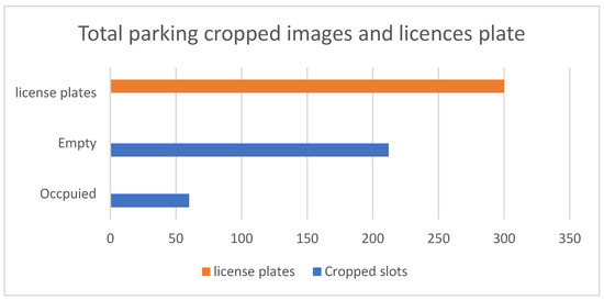
Figure 1.
Represents the total images from both datasets. The blue bars indicate the number of empty and occupied cropped images, while the orange bar represents the license plate images.
3.1. Dataset
Two datasets were used in the experimental method: one was for parking, and the other was for license plates. The parking dataset was manually created for the parking area at Islamia College Peshawar. A total of 11 full-size images were collected. It also included eight images of sunny conditions, with three images in rainy weather. Each image had dimensions of 1920 × 1080. Figure 1 shows different scenes from the parking yards based on sunny conditions. The slot areas were cropped from each image, with a total of 212 slot images in sunny conditions and 59 slot images in rainy conditions; a combination of both constituted a total of 272 slot images, which included both empty and occupied spaces. As a result, the dataset was imbalanced, with a low ratio of slot images. To address this, we applied two techniques—histogram equalization and augmentation, the rationale for which is discussed in the following section. Table 1 shows the total number of images in each class. An additional dataset consisting of 300 license plate images was downloaded from the internet.

Table 1.
Show the distribution of augmented parking dataset images into three phases: training, testing, and validation phases.
3.2. Pre-Processing
In the parking dataset, some images are affected by brightness due to being captured in the afternoon. As a result, the parking slots are not clearly visible, and the pixel values of both empty and occupied slots are very similar, making it challenging to train a model. Additionally, some parking spaces near the boundaries appear to be in the shadows of trees. When an end-user captures an image of a parking slot, it may not always be well-lit, which can hinder the model’s ability to accurately recognize the slot’s condition, potentially impacting the classification outcome [42]. These issues related to brightness and shadows are addressed using enhancement techniques, such as histogram equalization [43,44,45].
3.2.1. Histogram Equalization
Histogram equalization is a technique for enhancing images and plays a significant role in image processing [46]. Histogram-based strategies commonly operate uniformly throughout the image. However, the proposed method used this to adjust the contrast of the parking dataset images. Usually, histogram equalization only operates on grayscale images [47], not on RGB images. The traditional histogram algorithm for RGB images [48,49] was further improved and utilized to change the contrast of RGB images [50]. Numerous histogram techniques have been developed for RGB images and were introduced in [51]. We only used the basic histogram equalization method because it operates directly on the image.
An image was converted from RGB to YUV format before being processed with the histogram equalization algorithm. Although YUV is a color space, it is similar to the RGB color space model. A single YUV channel requires a traditional histogram equalization method for processing, which was already introduced in [52,53]. After completing the procedures, the slot image is converted into RGB format from the YUV color space. To maintain consistency throughout the dataset, we used a traditional histogram on all images of the parking dataset before submitting them to the model. Figure 2 shows the result of the histogram technique when applied to the cropped images. Figure 3 shows the result of the histogram equalization technique applied to the cropped images. Sub-images ‘a’ and ‘c’ represent the original images affected by poor lighting, while sub-images ‘b’ and ‘d’ show the enhanced images after applying histogram equalization.
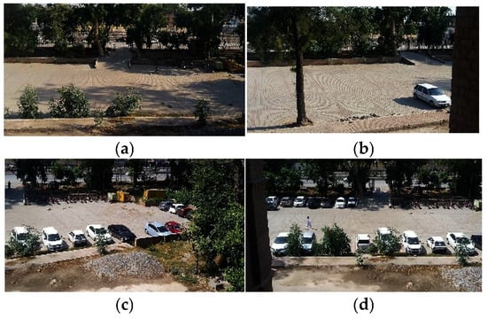
Figure 2.
Images of the parking area from different angles.
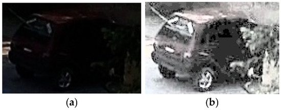
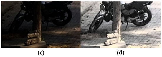
Figure 3.
Sub-images ‘(a)’ and ‘(c)’, which are original cropped images mostly affected by darkness. Sub-images ‘(b)’ and ‘(d)’ represent the results after applying the histogram equalization technique.
3.2.2. Augmentation
Before execution, we used rotation, height, and width shifting to augment the cropped images. When applying height and width shifting, each pixel in the image is transformed in the vertical and horizontal directions by a constant ratio. In our situation, a constant ratio existed between 0 and 0.2. The RGB values of the neighboring pixels are used to fill in the empty spaces, and any pixels that cross the border are ignored during shifting. The centroid pixel of the image is used as the reference point for rotation, with the rotation angle ranging from 0 to 20 degrees. As a result, applying the augmentation mechanism led to an imbalance in the dataset. The parking dataset is inherently imbalanced, causing the model to struggle with learning each class effectively. To address this, each image undergoes multiple augmentations, ensuring the model encounters a variety of differences in each epoch. The combined effect of the various augmentations used during the training, validation, and testing phases is illustrated in Figure 4.
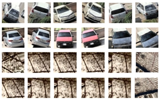
Figure 4.
Results of augmentation techniques—rotation, width shifting, and height shifting—applied to the cropped parking slot images in the dataset.
3.3. CNN Models
Deep learning is a core component of a large group of machine learning techniques [54,55,56]. It uses several hidden layers of deep learning to create classifiers that detect the essential low-level properties of an image that are variants of conventional neural network-based classifiers [57]. Many researchers have used the deep learning algorithm to solve problems in different domains because of its high precision in learning from objects compared to traditional machine learning techniques. Various types of deep learning were also discussed in [58]. One of the most well-known deep learning strategies is the convolutional neural network (CNN) introduced by [59] for handwritten recognition, which reliably trains several layers [60]. It has proven successful in various computer vision applications and is the most frequently used method. Convolutional neural networks consist of three fundamental layers: a convolutional layer, a max-pooling layer, and fully connected layers [61,62,63,64]. Following these strategies, many CNN models have been developed, such as LeNet [65], GoogleNet [66], AlexNet [67], VGG16, VGG19 [68], ResNet [69], DenseNet [70], SqueezeNet [71], Xception [72], Inception [73], EfficientNet [74], and MobileNet [75]. These models have been applied in the mechanism of detection [76,77,78,79,80,81], image classification [82,83,84,85], segmentation [86,87,88,89,90], robotic navigation [91,92], etc. However, the proposed method followed the concept of transfer learning. Transfer learning is a deep learning method that makes full use of features that the architecture has learned while addressing one issue to address a non-identical issue within the same domain. It offers several benefits [93,94,95], including the elimination of the need to design new model architecture, because it uses data that are already available from the prior training phase. The first benefit of transfer learning is that it saves computational time. The second is expanding the information obtained from previously trained models, and the third is that transfer learning is especially beneficial when the newly generated training dataset is very small. Transfer learning has contributed significantly to computer vision, audio classification, and natural language processing [96,97,98,99,100,101]. Especially in the image categorization task, multiple strides have been made to make it operate efficiently or precisely. Hence, the VGG16, Xception, and ResNet50 models’ primary architecture in the proposed method are pre-trained on the parking dataset, along with a CNN model.
3.3.1. Vgg16 Model
The Visual Geometry Group (VGG16) model was developed by Oxford researchers in 2014. It is trained on a large dataset, such as ImageNet, for classification purposes. The structure is based on convolution, pooling, and fully connected layers, including convolutions and one max-pooling layer in the first two phases. While three convolutions and one max-pooling layer are included in the last three phases. All blocks of the convolutional filter size are the same, and the sum of the filters is 64 in the first block of convolutional layers, the sum of the filters is 128 in the second block, the sum of the filters is 256 in the third block, and the sum of the filters in the last two blocks is 512. Once the feature extraction process is completed, the resulting feature map is flattened into a one-dimensional vector before being passed to the fully connected layer. The fully connected component contains three dense layers; the first two dense layers have 4096 neurons, while the last layer has 1000 neurons. Finally, activation functions such as softmax are used to output probabilities. This network’s sequential blocks, where successive convolutional layers are introduced one after the other, enable a decrease in the quantity of map data required. This is the advantage of this model. [102] used on the proposed dataset, and the outcome is good.
3.3.2. Resnet50 Model
In 2015, the residual network, ResNet, was developed and obtained 94.29% top five precision in opposition to the ImageNet dataset. There are multiple versions of ResNet, but in this experiment, we used ResNet50. It is a deep network with more convolutional layers than VGG16. The architecture has 50 layers, 48 convolutional layers, 1 max-pooling layer, and 1 average pooling layer [103]. The residual connection, a special connection between the convolutional layers that is subsequently transferred to the Relu activation layer, is one of its key features [104]. During backpropagation, the residual connection guarantees that the weights picked up from the prior layers do not vanish. The use of residual connections in this network, which allows for the utilization of numerous layers, is a major advantage. Furthermore, a deeper network (as opposed to a wider one) produces fewer additional parameters.
3.3.3. Xception Model
The Xception network is referred to as an extreme inception. This network comprises 14 modules that construct 36 convolutional layers for an extensive collection of features. When trained on the ImageNet dataset, the model achieved an accuracy of 94.95%. The key innovation of the Xception architecture is replacing the Inception module with a depth-wise separable convolution followed by a pointwise convolution. Since this network is a deep architecture, it enables more efficient computation than other deep models due to its fewer parameters, which is a major advantage.
3.3.4. Lenet Model
In 1989, Yan Yuan developed a convolutional neural network called lenient, which is also a term for LeNet5. This architecture involves two convolutional layers and two average pooling layers. After each convolution layer, there is an average pooling layer, followed by a dense layer with 84 nodes in the fully connected part. The main benefit is fast computation, as it does not have many deeper layers.
3.3.5. Alexnet Model
AlexNet was the first Convolutional Neural Network (CNN) architecture to participate in the 2012 ImageNet competition [105]. It surpassed all traditional methods and was used for image classification with a precision score of 84.60%. CNNs emerged as an advanced method for image classification. The AlexNet architecture contains three dense layers, five convolutional layers, and 60 million parameters. The use of dropout to prevent overfitting in this deep architecture, along with the ReLU activation function (as an alternative to the sigmoid function), are two novel features in AlexNet. Compared to other networks, this network’s primary benefit lies in its fast-training process. Nevertheless, the network must be sufficiently deep to extract intricate information from images.
3.3.6. MobileNet
MobileNet architecture was introduced and trained on an image dataset. Its purpose is to create a lightweight neural network model. MobileNet architecture is based on depth-wise separable and point-wise convolutions. The depth-wise separable convolution kernel operates on each image channel individually, and the point-wise convolution applies a 1 × 1 convolution to combine the outputs of the depth-wise convolution. The advantage of this model is that it has a small size, low latency in convolutional layers, can process data efficiently, and has fewer parameters than the deeper models.
3.3.7. Proposed CNN Model
The proposed CNN model architecture is shallow in terms of the number of layers, as shown in Figure 5. Unlike other CNN models such as VGG16, ResNet50, MobileNet, and Xception, it uses simple architecture. The feature extraction phase includes two convolutional layers, one depth-wise separable convolutional layer, and a max-pooling layer. One convolution occurs at the first layer, and another at the third layer, after the depth-wise separable convolution. Convolution is a matrix multiplication operation where the kernel values are multiplied with corresponding values; the result of this operation is illustrated in Figure 6. The depth-wise layer separates the image into three channels, such as red, green, and blue. Each channel is then multiplied with a filter. After this process, the three channels are recombined, and point convolution is applied. A 1 × 1 filter operates on the output of depth-wise convolution. Figure 7 shows the depth-wise separable convolution operation. All feature layers use the same configuration, with a kernel size of 3 × 3 and 32 filters. Figure 8 shows that max pooling plays a significant role in deep learning by reducing the dimensionality of features as it is applied to the feature maps. In the fully connected part of the model, there is only one dense layer with 64 neurons, followed by a sigmoid function for class probability output.
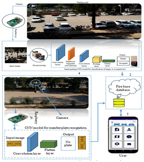
Figure 5.
Illustrates the proposed system architecture, where cameras capture parking images processed by Raspberry Pi for slot classification, and results are uploaded to the cloud. The mobile app enables users to request parking, while license plate recognition verifies vehicle access.
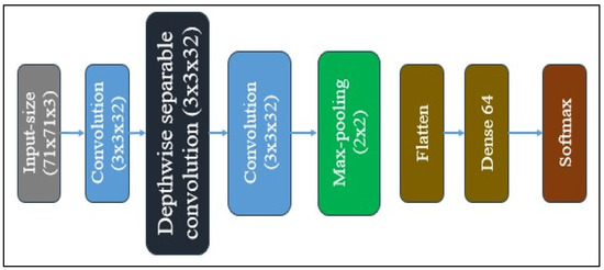
Figure 6.
Architecture of the proposed Convolutional Neural Network (CNN).
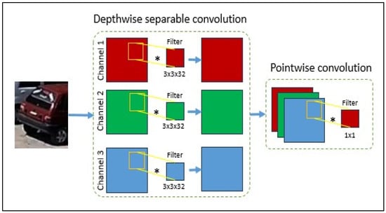
Figure 7.
Depth-wise separable convolution operation, image splits into three channel and applied 3 × 3 filter on individual channel then combined output applying 1 × 1 filter.
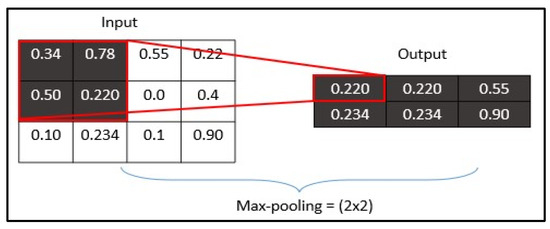
Figure 8.
Convolution process: a 2 × 2 filter multiplied with a 2 × 2-pixel region and result stores into output image.
In the experiment, fine-tuning was applied only to the fully connected part of the pre-trained models, where a dense layer of 64 neurons was added to adapt to the classification task. The input image size is 71 × 71 (RGB channels) instead of 224 × 224 × 3. Therefore, it requires less processing time. Another point is that not all image inputs are consistent with the parking dataset. There are two output classes: empty or occupied.
While models like VGG16 and ResNet50 are powerful, they are computationally intensive and not optimized for real-time inference on resource-constrained edge devices. Our custom CNN is intentionally designed to be lightweight, with significantly fewer parameters and lower computational requirements. For example, on Raspberry Pi, our model achieves similar classification accuracy to VGG16 but with a 70% reduction in inference time and memory usage. This makes it much more practical for real-world parking lot monitoring where hardware resources are limited.
3.4. Cloud Storage
Cloud storage is an internet-based technology that allows end-users to access and store data securely at any time and for extended periods [106]. As organizations grow, they require more devices, greater storage capacity, and complex management systems. Traditional methods involve regular backups, which consume both time and physical space, making them increasingly costly [107]. This need is addressed by cloud storage solutions. There are hundreds of different cloud storage services [108]. However, the proposed data, such as username, email, cell number, and vehicle plate number, is stored in Firebase Cloud.
3.5. Algorithm
Several heterogeneous algorithms have been developed to solve the problem. An algorithm is a finite sequence of steps designed to solve a specific problem. Researchers have widely applied various algorithms to find solutions; for example, Dijkstra’s algorithm, genetic algorithms, and K-Nearest Neighbors (K-NN) have been used to estimate the shortest distance. In computer science, algorithms are applied across diverse problem areas such as network communication, shortest path computation, and road navigation, depending on the nature of the problem. This experiment employed the merge sort algorithm. Although several sorting algorithms are available, the merge sort was chosen due to its efficient worst-case time complexity of O (n log n) [109,110], which makes it suitable for searching through records. Merge sorts follow a divide-and-conquer approach. In the first phase, it recursively divides the list into halves until each sub-list contains a single element. In the second phase, it merges these sub-lists by comparing elements, eventually producing a fully sorted list [111]. As described, merge sort techniques are used in the proposed method behind the mobile application. During this time, the distance list that was obtained was unsorted. The list is processed using the merge sort algorithm, which outputs a sorted list upon completion. In this sorted list, the first index represents the nearest parking location, with each subsequent index indicating a progressively greater distance. The final index corresponds to the farthest parking spot. Figure 9 illustrates the concept of the merge sort algorithm.
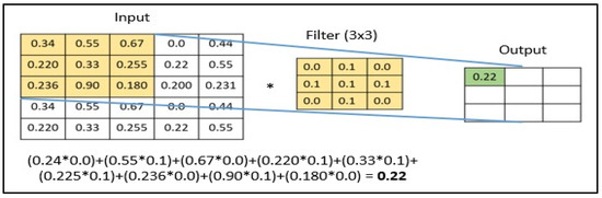
Figure 9.
Max-pooling process: a 3 × 3 filter finds the maximum pixel value and stores it in the output image.
4. Experiment Result
In this phase, the mobile application user interface is presented, emphasizing key functionalities that facilitate user interaction. Furthermore, the performance of the pretrained model is evaluated using a confusion matrix across different datasets to assess its generalization ability. Several baseline parameters—such as accuracy and model size—are also compared to determine overall effectiveness.
4.1. Mobile Application
Mobile applications are software programs designed to run on mobile devices, providing end-users with access to essential services. Commonly referred to as mobile apps or simply apps, they are widely used and often developed for specific functionalities. In the context of smart parking, dedicated mobile applications have been designed to support parking-related services. This app offers faster performance compared to its web-based counterpart. Given the widespread use of mobile devices, with users remaining connected around the clock, the app enables real-time access to information regarding the nearest available parking lots. Before using the app, end-users are required to register and log in. Once logged in, they can access a variety of features displayed on the mobile interface. Thus, these coordinates are entered into the distance function to find the distance between the user and the parking space, as illustrated in Figure 10, which demonstrates the steps of the Merge Sort algorithm used to sort the distances.
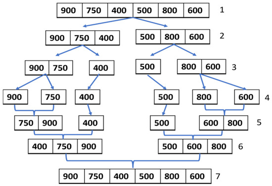
Figure 10.
Merge sort algorithm steps. Step 1 is a found distance in unsorted form. Steps 2–3 split the list into halves; in step 4, each unit is no longer divisible. Steps 5–6 perform reverse merging, and step 7 produces the final sorted list.
It has several functions, such as ‘request’, information’, ‘map’, ‘setting’, ‘profile’, and ‘around info’. These functions are mentioned in the bulleted form, and Figure 11 depicts app pages.
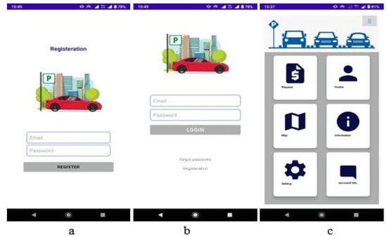
Figure 11.
Shows the mobile application pages: ‘(a)’ is the registration page, ‘(b)’ is the login page, and ‘(c)’ is the menu page.
- Behind the process, the ‘request’ function is based on the service of the nearest parking location and then the closest slot. Suppose the user wants space for a standing vehicle in the parking lot; then they click on the ‘request’ event. Then, the mobile GPS is automatically turned on to find the user’s current coordinates. This way, the parking coordination is stored in cloud storage. Thus, these coordinates are put in the distance function to find the distance between the user and the parking space. The outcomes of the distance function are kept in an array. The merge sort algorithm is used to sort the data after the distance has been found, since there are multiple parking distances between the parking spaces and the users. The element in the first index, the nearest parking distance location, will be shown on the screen.
- The user’s name, phone number, and license plate number are available on the profile page.
- The information page shows details about the reservation space and the parking space.
- In the settings page, include the change password and email events.
- The map page shows the map and navigation options.
- The info page describes the information that surrounds the parking.
4.2. Evaluation of Models Using the Confusion Matrix and Classification Measures
Table 1 describes the distribution of the parking dataset. The dataset is divided into three phases: training, testing, and validation. In the training phase, 60% of samples of both classes are used during the execution time of the training model, while in the testing phase, 20% of samples are used and 20% are reserved for validation. Samples from the testing 470 phase are treated as new data and used after the training to evaluate the model generalization. So, to check the model’s perception on validation images, two other datasets were used to test all proposed models, which were trained on the parking dataset. The CNR + EXT dataset and PKLot dataset, specifically the UFPR04 and UFPR05 subsets. Confusion matrices are widely used for estimation when attempting to solve classification issues. They can solve both binary and multiclass classification issues. Table 2 illustrates a confusion matrix for binary classification.
Table 2.
Confusion matrix for binary classification.
Confusion matrices show counts between expected and actual labels. The result “TN” stands for True Negative and displays the number of negatively classed cases that were correctly identified. Similarly, “TP” stands for True Positive and denotes the quantity of correctly identified positive cases. The abbreviation “FP” denotes false positive, i.e., the number of negative cases incorrectly categorized as positive, while “FN” denotes false negative, i.e., the number of positive cases incorrectly categorized as negative.
Since accuracy might be deceptive when applied to unbalanced datasets, alternative metrics based on the confusion matrix are also relevant for assessing performance. The “confusion matrix” method from the “sklearn” module in Python 3.8 can be used to obtain the confusion matrix. The command “from sklearn. metrics import confusion_matrix” can be used to import this function into Python 3.8. Users must supply the function with actual and predicted values to obtain the confusion matrix. The classification measure contains terms such as precision, recall, F1-score, etc., extending the confusion matrix. Precision is a matrix term; it identifies the true positive label prediction in the quantity form out of all actual true positive labels. Thus, true positive labels predicted through the model are divided by the sum of the predicted true positive and false positive labels.
Equation (2) represents a precision process. TP stands for true positive label, while FP stands for false positive. Recall is a term of the true positive matrix; it identifies the true positive label prediction as a quantity out of all true positive labels. Thus, true positive la-bels predicted through the model are divided by the sum of predicted true positive and false negative labels.
Equation (3) represents the recall process; TP stands for true positive, while FN stands for false negative. A classifier’s recall and precision scores are combined to create the F-measure, sometimes called the F-value. In classification situations, the F-measure is another often-used statistic. A weighted average of recall and precision is used to get the F-measure. It is helpful to comprehend the trade-off between precision and coverage when classifying a positive situation.
Equation (4) represents the F1-score process. The F1-score is calculated as the harmonic mean of precision and recall, using the formula: F1 = 2 × (precision × recall)/(precision + recall).
In this section, the performance of the proposed pre-trained model of individual class is analyzed in terms of precision, recall, and F1-score based on the validation images, as demonstrated in Table 3. The Vgg16, Resnet50, Xception, and Lenet models have the same score; these models have a precision value of 99.97%, a recall value of 100.0%, and an F1 value of 99.98%. In the empty class, the precision score is 100.0%, the recall is 99.92%, and the F1 value is 99.96%. Similarly, MobileNet and the proposed CNN model have the same score for all terms, 100.0%, and higher than other models, while the AlexNet model’s score is less than that of all other models. The precision, recall, and F1-score for the empty class are 99.97%, while for the occupied class, these metrics are 99.92%. These results indicate strong performance and validate the effectiveness of both the MobileNet and the proposed CNN model on the test images. Another analysis of the performance of the pre-trained architecture of individual classes in terms of precision, recall, and F1-score on the UERE04 and UFPR05 datasets. UFPR04 and UFPR05 are subsets of the PkLot da-taset. The PkLot dataset contains 12,417 full images of parking yards in different weather conditions, such as overcast, sunny, and rainy. The total number of cropped images of slot areas is 695,899 from all the empty or occupied images. The subset of UFPR04 empty class images is 59,718, and occupied class images are 46,125, so the total number of images for both classes is 105,843, while a subset of UFPR05 has a total of 165,785 images: 68,359 empty class images, and 97,426 occupied class images; these subsets are detailed in Table 4. In Table 5, The Vgg16 model’s high score is 99.54% in terms of precision based on the empty class, while on the occupied class outcome value is 99.84% in terms of recall.; Likewise, while observing the performance of the ResNet50 model performs similarly to VGG16, showing strong results only in terms of precision for the empty class and recall for the occupied class. However, both models underperform compared to others when evaluated using the F1-score for both classes. In contrast, the MobileNet and Xception models demonstrate a strong likelihood of superior performance, with only a 0.5 to 0.7 difference in F1-scores between them. The proposed CNN model and LeNet follow as the second-best performers, achieving up to 80% across all classification metrics. LeNet alone ranks third, scoring slightly below 80% on all metrics. In Table 6, the MobileNet model has the highest precision score on the empty class and recall score on the occupied class, in the same way as the model of Lenet and the proposed CNN. In terms of the F1-score, the Xception model performs particularly well on the occupied class, due to its high precision and recall. On the other hand, AlexNet and the other models show varying performance, with some models exhibiting lower or higher precision, recall, and F1-scores across both classes. The third analysis is the performance of the pre-trained models on the CNR + EXT dataset. The CNRPPark + EXT is an extension of the CNRPark dataset. It has 4287 full images taken on 23 different days with three weather scenarios: overcast, sunny, and rainy. The full images are cropped to extract the slot parts, resulting in a total of 144,965 slot images—comprising 65,658 images of empty slots and 79,307 images of occupied slots. The CNR + EXT details are mentioned in Table 7.
Table 3.
Details of three different parking datasets, including the number of images per class and the total number of images, categorized by various weather conditions such as sunny, cloudy, and rainy.
Table 4.
Represents the precision, recall, and F1-score performance based on the validation images of the proposed parking dataset.
Table 5.
Represents the precision, recall, and F1-score performance based on the UFPR04 dataset images.
Table 6.
Represents terms of precision, recall, and F1-score performance based on the UFPR05 dataset images.
Table 7.
Represents the terms of precision, recall, and F1-score performance based on the CNR dataset images.
4.3. Comparison of Proposed Models
The comparative analysis of seven experiment-trained models, such as LeNet, AlexNet, Xception, VGG16, MobileNet, and ResNet50, as well as the proposed CNN, revealed in Table 8, is based on model size and computational cost for smart parking applications.
Table 8.
Comparison of accuracy and model size of the proposed architecture.
Among the heavyweight models, Xception and VGG16 achieved high accuracy on the proposed dataset (99.97%) and strong generalization on benchmark datasets (e.g., 97.18% for UFPR04 with Xception). However, this comes at the cost of large model sizes (239.6 MB and 170.1 MB, respectively) and extremely high computational requirements (1103.36 MFLOPs for Xception, 2766.89 MFLOPs for VGG16). These models, though accurate, are unsuitable for edge deployment due to latency and hardware constraints.
ResNet50 also shows decent accuracy (99.97%) but suffers from a large model size (283.9 MB) and high MFLOPs (986.03), placing it in a similar category as VGG16 and Xception in terms of inefficiency for real-time embedded systems.
MobileNet, designed for lightweight applications, performs well with high accuracy (97.24% on UFPR04 and 100% on the proposed dataset), a moderate model size (40.2 MB), and relatively low MFLOPs (101.99). It proves to be a strong contender for smart parking on resource-constrained devices.
LeNet, the smallest traditional architecture in terms of computation (8.93 MFLOPs) and size (4.5 MB), delivers moderate performance (87.77% on UFPR04), making it suitable for simpler deployments where top-tier accuracy is not required.
The proposed CNN model, with only 2 MB size and 20.15 MFLOPs, achieves 100% accuracy on the custom dataset and performs comparably on public datasets like UFPR04 (83.64%) and UFPR05 (84.46%). While it may not outperform complex models on all datasets, its balance between accuracy and computational efficiency makes it ideal for real-time edge deployment in smart parking systems.
4.4. Brief Discussion Based on the Detection and Classification Model
In this section, the discussion is about the detection and classification model. The classification model is a model that predicts class labels. Its architecture is based on two main parts: the feature extraction part, which includes convolutional, pooling, stride, dropout, and ReLU function layers, and the other is the fully connected part, which involves dense layers, and the final layer is equipped with an activation function. This model takes an image as input and outputs a class label that belongs to a specific class group. There are a lot of generated classification models that are trained on massive datasets. In detection models, the input image is processed not only for classification but also for the localization (and sometimes orientation) of the object. It has a similar architecture to the classifier but includes an additional head section for the localization process. Multiple detection concepts are available, like YOLO [112], SSD [113], R-CNN [114], Faster R-CNN, LSTM, 1D-CNN, Decision Tree [115,116,117,118,119,120,121], window sliding [122], etc., and they are widely used to solve detection problems. If both models are compared according to the architecture, processing time, and outcome, the classifier architecture predicts the class label. For example, if an object is small or located at the top left side of the image, the classifier still predicts only the class of the whole image; regardless of object detection location, it classifies the whole image. Its computational time is less than that of the detection model. One detection scenario includes a feature extraction component called the backbone. Another component is the detection head, which focuses on the concept of object detection. It is efficient in generating output, as it classifies objects and provides their position or localization within the image. However, due to the added complexity of detection, it requires significantly more computational resources and takes longer to process than the classifier alone. However, the proposed CNN model is a classifier; all the dataset images have been manually annotated for the slot area, whether empty or occupied. Therefore, in the experiment method, cameras are fixed in the parking area, not for surveillance. All annotated slots in every image are passed to the classifier for prediction in the detection process. Then, a bounding box is drawn at the slot position in the image, annotated with a label and score. Figure 12 shows detection process and Figure 13 shows the validation performance of proposed CNN.
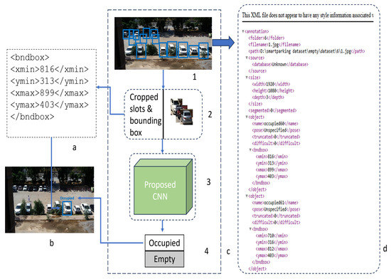
Figure 12.
Shown detection process.
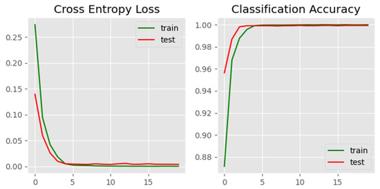
Figure 13.
Training and validation performance of the proposed CNN model.
To ensure transparency and reproducibility of the proposed CNN model, we present its key hyperparameters in Table 9. The model accepts input images of size 71 × 71 × 3 and is composed of two Conv2D layers, one DepthwiseConv2D layer, a single MaxPooling2D layer, and a fully connected Dense layer. ReLU is used as the activation function throughout the network. The model is trained using the Adam optimizer with a learning rate of 0.001 and a batch size of 128. These parameters were selected after empirical tuning to strike a balance between computational efficiency and performance, particularly for edge device deployment. The simplicity of the architecture and optimized training settings contribute to reduced model size and lower inference latency, making it suitable for real-time parking applications on resource-constrained platforms.
Table 9.
Hyperparameters of proposed CNN model.
To provide evidence of the convergence and stability of the proposed CNN model, we include training and validation performance plots in Figure 13. The consistent decline in cross-entropy loss and simultaneous rise and stabilization of accuracy curves indicate effective convergence during training. These empirical results demonstrate the model’s reliability and generalization, serving as a practical alternative to formal convergence proofs typically used in numerical methods.
4.5. Error Analysis
Although the proposed CNN model demonstrates high accuracy and a compact size suitable for edge deployment, some limitations remain, particularly under real-world conditions not represented in the training dataset. The model exhibited false positives that occurred on images affected by shadows, partial occlusions, and artificial lighting, such as red lamps or reflective surfaces (Figure 14a–d). These environmental factors were not present in the custom training dataset, which primarily contained well-lit, unobstructed parking slots. As a result, the model lacked exposure to such challenging conditions, leading to misclassifications. For example, shadows cast by vehicles or surrounding objects were sometimes misclassified as occupied slots, and glare from lamps or bulbs caused the model to incorrectly detect vehicle presence. Furthermore, because of this limited environmental diversity in the training data, the model may have developed biases toward clean visual patterns, reducing its ability to generalize in less controlled scenarios.
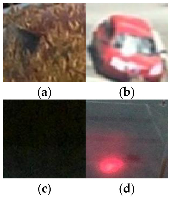
Figure 14.
Misclassification by the proposed CNN model.
4.6. Discussion
The experimental results across multiple datasets demonstrate that the proposed CNN model performs competitively, achieving 100% accuracy on the proposed parking dataset and delivering satisfactory results on public datasets such as UFPR04, UFPR05, and CNRPark-EXT. These results indicate that the proposed model is capable of effectively identifying parking slot conditions in diverse scenarios. As shown by the proposed model performance Figure 15 sunny conditions and Figure 16 shows the rainy conditions.
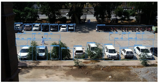
Figure 15.
Shows the performance of the proposed CNN model in a sunny scene.
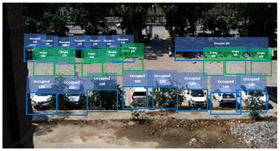
Figure 16.
Shows the performance of the proposed CNN model in a rainy scene.
A key advantage of the proposed CNN architecture lies in its compact size and low computational complexity. Compared to deeper and more resource-intensive models like VGG16, ResNet50, and Xception, the proposed CNN offers a more efficient solution suitable for deployment on edge devices such as Raspberry Pi. This makes it ideal for real-time applications in smart parking systems where speed, efficiency, and hardware constraints are critical.
However, the model has certain limitations. In public datasets such as CNRPark-EXT and UFPR05, the performance slightly declines due to challenging image conditions. These include visual obstructions (e.g., trees or lamp posts), shadows on occupied slots, improper cropping, and variations in lighting and weather. These issues make it difficult for the model to generalize across diverse environments.
To address these challenges, future work may explore the following directions:
- Incorporating data from different perspectives and environmental conditions to improve model robustness.
- Using attention mechanisms or adaptive preprocessing techniques to enhance feature extraction in low-visibility conditions.
- Integrating semantic segmentation or object detection to better localize and understand parking slots.
Table 10 shows a comparison of the performances of several models on the PKLot dataset in terms of accuracy and model size. The proposed CNN model was tested on the Full PKLot dataset images, unlike previous works [123,124,125]) that tested only on distributed subsets of the dataset. Despite this comprehensive testing, the proposed CNN achieved an accuracy of 84.04% with a significantly smaller model size (2.00 MB), highlighting its efficiency and suitability for edge devices. On the custom proposed dataset, the same model achieved 100.0% accuracy, confirming its strong performance under controlled conditions.
Table 10.
Comparison with previous work based on accuracy and model size.
5. Conclusions
This article focuses on identifying the nearest available parking space using a custom-built parking dataset and deep learning techniques. In the experimental study, six widely used pre-trained models—VGG16, ResNet50, MobileNet, LeNet, AlexNet, and Xception—were evaluated through transfer learning. Additionally, a lightweight, custom-designed CNN model was proposed and tested on the same dataset. A mobile application was also developed to provide real-time parking information to users. The backend of the application employs a merge sort algorithm to efficiently sort parking spaces based on distance, helping to reduce traffic congestion, save time and fuel, and lower CO2 emissions.
Future work will focus on enhancing the dataset by incorporating images under diverse weather and lighting conditions, such as overcast, foggy, and nighttime scenarios, which are currently underrepresented. The current binary classification task (occupied vs. free) will be expanded to handle more nuanced cases, including reserved spaces, illegally parked vehicles, and misaligned parking. The distance estimation will be refined to consider route-based navigation rather than straight-line distances. Additional features planned for the mobile application include time tracking, integrated payment systems, real-time notifications, and improved user authentication—potentially incorporating biometric security like fingerprint verification. Further exploration of advanced deep learning techniques is also planned to improve robustness and accuracy across varied environments.
Author Contributions
Conceptualization, M.O.K., M.A.R. and M.A.I.M.; methodology, M.O.K., M.A.R., M.A.I.M. and R.I.S.; software, I.U.A.; validation, M.A.I.M., M.O.K. and R.I.S.; formal analysis, M.A.I.M. and R.I.S.; investigation, M.A.I.M. and H.C.K.; resources, M.A.I.M.; data curation, M.A.I.M.; writing—original draft preparation, M.A.I.M.; writing—review and editing, M.A.I.M., M.O.K. and M.A.R.; visualization, M.A.I.M.; supervision, M.A.I.M. and H.C.K.; project administration, M.A.I.M. and H.C.K. All authors have read and agreed to the published version of the manuscript.
Funding
This research received no external funding.
Data Availability Statement
Data can be given upon request to the corresponding author.
Conflicts of Interest
The authors declare no conflicts of interest.
References
- Lin, T.; Hervé, R.; Frédéric, L.M. A survey of smart parking solutions. IEEE Trans. Intell. Transp. Syst. 2017, 18, 3229–3253. [Google Scholar] [CrossRef]
- Tang, C.; Wei, X.; Zhu, C.; Chen, W.; Rodrigues, J.J.P.C. Towards smart parking based on fog computing. IEEE Access 2018, 6, 70172–70185. [Google Scholar] [CrossRef]
- Min, K.-W.; Choi, J.-D. Design and implementation of autonomous vehicle valet parking system. In Proceedings of the 16th International IEEE Conference on Intelligent Transportation Systems (ITSC 2013), Hague, The Netherlands, 6–9 October 2013; pp. 2082–2087. [Google Scholar]
- 2018. Available online: https://spectrum.ieee.org/the-big-problem-with-selfdriving-cars-is-people (accessed on 10 December 2024).
- Nayak, A.K.; Akash, H.C.; Prakash, G. Robotic valet parking system. In Proceedings of the 2013 Texas Instruments India Educators’ Conference, Washington, DC, USA, 4–6 April 2013; pp. 311–315. [Google Scholar]
- Valipour, S.; Siam, M.; Stroulia, E.; Jagersand, M. Parking-stall vacancy indicator system, based on deep convolutional neural networks. In Proceedings of the 2016 IEEE 3rd World Forum on Internet of Things (WF-IoT), Reston, VA, USA, 12–14 December 2016; pp. 655–660. [Google Scholar]
- Amato, G.; Carrara, F.; Falchi, F.; Gennaro, C.; Meghini, C.; Vairo, C. Deep learning for decentralized parking lot occupancy detection. Expert Syst. Appl. 2017, 72 (Suppl. C), 327–334. [Google Scholar] [CrossRef]
- Nithya, R.; Priya, V.; Sathiya Kumar, C.; Dheeba, J.; Chandraprabha, K. A Smart Parking System: An IoT Based Computer Vision Approach for Free Parking Spot Detection Using Faster R-CNN with YOLOv3 Method. Wirel. Pers. Commun. 2022, 125, 3205–3225. [Google Scholar] [CrossRef]
- Ahad, A.; Kidwai, F.A. YOLO based approach for real-time parking detection and dynamic allocation: Integrating behavioral data for urban congested cities. Innov. Infrastruct. Solut. 2025, 10, 252. [Google Scholar] [CrossRef]
- Shen, T.; Hua, K.; Liu, J. Optimized public parking location modelling for green intelligent transportation systems using genetic algorithms. IEEE Access 2019, 7, 176870–176883. [Google Scholar] [CrossRef]
- Öncevarlıkl, D.F.; Yıldız, K.D.; Gören, S. Deep Learning Based On-Street Parking Spot Detection for Smart Cities. In Proceedings of the 2019 4th International Conference on Computer Science and Engineering (UBMK), Samsun, Turkey, 11–15 September 2019; pp. 177–182. [Google Scholar] [CrossRef]
- Di Mauro, D.; Furnari, A.; Patanè, G.; Battiato, S.; Farinella, G.M. Estimating the occupancy status of parking areas by counting cars and non-empty stalls. J. Vis. Commun. Image Represent. 2019, 62, 234–244. [Google Scholar] [CrossRef]
- Ata, K.M.; Soh, A.C.; Ishak, A.J.; Jaafar, H.; Khairuddin, N.A. Smart Indoor Parking System Based on Dijkstra’s Algorithm. Int. J. Integr. Eng. 2019, 2, 13–20. [Google Scholar]
- Wang, H.; Zhang, F.; Cui, P. A parking lot induction method based on Dijkstra algorithm. In Proceedings of the 2017 Chinese Automation Congress (CAC), Jinan, China, 20–22 October 2017; IEEE: Piscataway, NJ, USA, 2017; pp. 5247–5251. [Google Scholar]
- Aydin, I.; Karakose, M.; Karakose, E. A navigation and reservation based smart parking platform using genetic optimization for smart cities. In Proceedings of the 2017 5th International Istanbul Smart Grid and Cities Congress and Fair (ICSG), Istanbul, Turkey, 19–21 April 2017; IEEE: Piscataway, NJ, USA, 2017; pp. 120–124. [Google Scholar]
- Yousaf, K.; Duraijah, V.; Gobee, S. Smart parking system using vision system for disabled drivers (OKU). ARPN J. Eng. Appl. Sci. 2016, 11, 3362–3365. [Google Scholar]
- Ahmed, S.; Rahman, M.S.; Rahaman, M.S. A blockchain-based architecture for integrated smart parking systems. In Proceedings of the 2019 IEEE International Conference on Pervasive Computing and Communications Workshops (PerCom Workshops), Kyoto, Japan, 11–15 March 2019; IEEE: Piscataway, NJ, USA, 2019; pp. 177–182. [Google Scholar]
- Vakula, D.; Kolli, Y.K. Low cost smart parking system for smart cities. In Proceedings of the 2017 International Conference on Intelligent Sustainable Systems (ICISS), Palladam, India, 7–8 December 2017; IEEE: Piscataway, NJ, USA, 2017; pp. 280–284. [Google Scholar]
- Roman, C.; Liao, R.; Ball, P.; Ou, S.; de Heaver, M. Detecting on-street parking spaces in smart cities: Performance evaluation of fixed and mobile sensing systems. IEEE Trans. Intell. Transp. Syst. 2018, 19, 2234–2245. [Google Scholar] [CrossRef]
- Lee, C.; Han, Y.; Jeon, S.; Seo, D. Smart parking system for Internet of Things. In Proceedings of the 2016 IEEE International Conference on Consumer Electronics (ICCE), Las Vegas, NV, USA, 7–11 January 2016; IEEE: Piscataway, NJ, USA, 2016. [Google Scholar]
- Cheng, Y.; Li, F.; Chen, J.; Ji, W. A smart parking system using WiFi and wireless sensor network. In Proceedings of the 2016 IEEE International Conference on Consumer Electronics-Taiwan (ICCE-TW), Nantou, Taiwan, 27–29 May 2016; IEEE: Piscataway, NJ, USA, 2016. [Google Scholar]
- Varghese, A.; Sreelekha, G. An Efficient Algorithm for Detection of Vacant Spaces in Delimited and Non-Delimited Parking Lots. IEEE Trans. Intell. Transp. Syst. 2019, 21, 4052–4062. [Google Scholar] [CrossRef]
- Goswami, P.; Pokhriyal, B.; Kumar, K. On the Solution of Two-Dimensional Local Fractional LWR Model of Fractal Vehicular Traffic Flow. Appl. Math. 2024, 4, 1–14. [Google Scholar] [CrossRef]
- Elgezouli, D.E.; Abdoon, M.A.; Belhaouari, S.B.; Almutairi, D.K. A Novel Fractional Edge Detector Based on Generalized Fractional Operator. Appl. Math. 2024, 4, 1009–1028. [Google Scholar] [CrossRef]
- Liu, K.; Zhang, X.; Chen, Y. Energy Informatics and Fractional Calculus. In Proceedings of the ASME 2017 International Design Engineering Technical Conferences and Computers and Information in Engineering Conference, Cleveland, OH, USA, 6–9 August 2017. [Google Scholar] [CrossRef]
- Sun, H.; Zhang, Y.; Baleanu, D.; Chen, W.; Chen, Y. A New Collection of Real World Applications of Fractional Calculus in Science and Engineering. Appl. Math. 2018, 3, 213–231. [Google Scholar] [CrossRef]
- Smart Parking Ltd. Smart Parking Annual Report FY24. Available online: https://www.smartparking.com/uk/ (accessed on 10 December 2024).
- Singh, K.I.; Khan, M.I.; Singh, I.T. Applications of Fractional Calculus. Appl. Math. 2023, 3, 256–271. [Google Scholar]
- Mehta, P.P.; Fernandez, A.; Rozza, G. Fractional Calculus Seminar Series; SISSA MathLab: Trieste, Italy, 2024; Available online: https://mathlab.sissa.it/fractional-calculus-seminars (accessed on 10 December 2024).
- Singh, P.; Parihar, S. Smart Parking Systems: A Review of Technologies and Benefits. Int. J. Commun. Netw. Inf. Secur. 2024, 16, 862–879. [Google Scholar]
- Chen, Q.; Chen, T.; Yu, H.; Song, J.; Liu, D. Lateral Control for Autonomous Parking System with Fractional Order Controller. J. Softw. 2011, 6, 1075–1081. [Google Scholar] [CrossRef][Green Version]
- Singh, H.; Srivastava, H.M.; Nieto, J.J. (Eds.) Handbook of Fractional Calculus for Engineering and Science; CRC Press: Boca Raton, FL, USA, 2022. [Google Scholar] [CrossRef]
- Magin, R.L. Fractional Calculus in Bioengineering. Crit. Rev. Biomed. Eng. 2004, 32, 1–104. [Google Scholar] [CrossRef]
- Failla, G.; Zingales, M. Advanced Materials Modelling via Fractional Calculus: Challenges and Perspectives. Philos. Trans. R. Soc. A Math. Phys. Eng. Sci. 2020, 378, 20200050. [Google Scholar] [CrossRef]
- Wang, Q.; Li, C.; Zhan, G.; Zhu, W. A Novel Fractional Order Partial Grey Model for Forecasting Short-Term Traffic Flow. J. Comput. Des. Eng. 2025, 12, 218–234. [Google Scholar] [CrossRef]
- Flores, C.; Muñoz, J.; Monje, C.A.; Milanés, V.; Lu, X.-Y. Iso-damping Fractional-Order Control for Robust Automated Car-Following. J. Adv. Res. 2020, 25, 181–189. [Google Scholar] [CrossRef]
- Coelho, C.; Costa, M.F.P.; Ferrás, L.L. Fractional Calculus Meets Neural Networks for Computer Vision: A Survey. AI 2024, 5, 1391–1426. [Google Scholar] [CrossRef]
- Safouan, S.; El Moutaouakil, K.; Patriciu, A.-M. Fractional Derivative to Symmetrically Extend the Memory of Fuzzy C-Means. Symmetry 2024, 16, 1353. [Google Scholar] [CrossRef]
- Mathur, A.; Akhtar, A. Fractional Calculus in Signal Processing: The Use of Fractional Calculus in Signal Processing Applications Such as Image Denoising, Filtering, and Time Series Analysis. Int. J. Multidiscip. Res. 2023, 5, 23045469. [Google Scholar]
- Tarasov, V.E. Mathematical Economics: Application of Fractional Calculus. Mathematics 2020, 8, 660. [Google Scholar] [CrossRef]
- Li, Y.; Lu, H.; Li, J.; Li, X.; Li, Y.; Serikawa, S. Underwater image de-scattering and classification by deep neural network. Comput. Electr. Eng. 2016, 54, 68–77. [Google Scholar] [CrossRef]
- Cheng, H.-D.; Shi, X.J. A simple and effective histogram equalization approach to image enhancement. Digit. Signal Process. 2004, 14, 158–170. [Google Scholar] [CrossRef]
- Sim, K.; Tso, C.; Tan, Y. Recursive sub-image histogram equalization applied to gray scale images. Pattern Recognit. Lett. 2007, 28, 1209–1221. [Google Scholar] [CrossRef]
- Patel, S.; Goswami, M. Comparative analysis of Histogram Equalization techniques. In Proceedings of the 2014 International Conference on Contemporary Computing and Informatics (IC3I), Mysore, India, 27–29 November 2014; IEEE: Piscataway, NJ, USA, 2015; pp. 167–168. [Google Scholar]
- Ahmed, S.; Hasan, B.; Ahmed, T.; Sony, R.K.; Kabir, H. Less is More: Lighter and Faster Deep Neural Architecture for Tomato Leaf Disease Classification. IEEE Access 2022, 10, 68868–68884. [Google Scholar] [CrossRef]
- Han, J.-H.; Yang, S.; Lee, B.-U. A Novel 3-D Color Histogram Equalization Method with Uniform 1-D Gray Scale Histogram. IEEE Trans. Image Process. 2010, 20, 506–512. [Google Scholar] [CrossRef]
- Hsu, W.-Y.; Chou, C.-Y. Medical Image Enhancement Using Modified Color Histogram Equalization. J. Med Biol. Eng. 2015, 35, 580–584. [Google Scholar] [CrossRef]
- Hsu, W.-Y.; Zuo, X.-N. Registration Accuracy and Quality of Real-Life Images. PLoS ONE 2012, 7, e40558. [Google Scholar] [CrossRef] [PubMed]
- Kim, T.K.; Paik, J.K.; Kang, B.S. Contrast enhancement system using spatially adaptive histogram equalization with temporal filtering. IEEE Trans. Consum. Electron. 1998, 44, 82–87. [Google Scholar]
- Hsu, W.-Y.; Abbott, D. A Practical Approach Based on Analytic Deformable Algorithm for Scenic Image Registration. PLoS ONE 2013, 8, e66656. [Google Scholar] [CrossRef]
- Li, Z.; Wei, Z.; Wen, C.; Zheng, J. Detail-Enhanced Multi-Scale Exposure Fusion. IEEE Trans. Image Process. 2017, 26, 1243–1252. [Google Scholar] [CrossRef]
- Stanescu, D.; Stratulat, M.; Groza, V.; Ghergulescu, J.; Borca, D. Steganography in YUV color space. In Proceedings of the 2007 International Workshop on Robotic and Sensors Environments, Ottawa, ON, Canada, 12–13 October 2007; IEEE: Piscataway, NJ, USA, 2007; pp. 1–4. [Google Scholar]
- Jia, X. Image recognition method based on deep learning. In Proceedings of the 2017 29th Chinese Control and Decision Conference (CCDC), Chongqing, China, 28–30 May 2017; pp. 4730–4735. [Google Scholar] [CrossRef]
- Du, X.; Cai, Y.; Wang, S.; Zhang, L. Overview of deep learning. In Proceedings of the 2016 31st Youth Academic Annual Conference of Chinese Association of Automation (YAC), Wuhan, China, 11–13 November 2016; pp. 159–164. [Google Scholar] [CrossRef]
- Kamilaris, A.; Boldú, F.X.P. Deep learning in agriculture: A survey. Comput. Electron. Agric. 2018, 147, 70–90. [Google Scholar] [CrossRef]
- Heaton, J.; Goodfellow, I.; Bengio, Y. Aaron Courville: Deep Learning. Genet. Program. Evolvable Mach. 2018, 19, 305–307. [Google Scholar] [CrossRef]
- Janiesch, C.; Zschech, P.; Heinrich, K. Machine learning and deep learning. Electron. Mark. 2021, 31, 685–695. [Google Scholar] [CrossRef]
- LeCun, Y.; Boser, B.; Denker, J.S.; Henderson, D.; Howard, R.E.; Hubbard, W.; Jackel, L.D. Backpropagation Applied to Handwritten Zip Code Recognition. Neural Comput. 1989, 1, 541–551. [Google Scholar] [CrossRef]
- Vincent, P.; Larochelle, H.; Lajoie, I.; Bengio, Y.; Manzagol, P.-A.; Bottou, L. Stacked denoising autoencoders: Learning useful representations in a deep network with a local denoising criterion. J. Mach. Learn. Res. 2010, 11, 3371–3408. [Google Scholar]
- O’Shea, K.; Nash, R. An introduction to convolutional neural networks. arXiv 2015, arXiv:1511.08458. [Google Scholar]
- Albawi, S.; Mohammed, T.A.; Al-Zawi, S. Understanding of a convolutional neural network. In Proceedings of the 2017 International Conference on Engineering and Technology (ICET), Antalya, Turkey, 21–23 August 2017; pp. 1–6. [Google Scholar] [CrossRef]
- Gu, J.; Wang, Z.; Kuen, J.; Ma, L.; Shahroudy, A.; Shuai, B.; Liu, T.; Wang, X.; Wang, G.; Cai, J.; et al. Recent advances in convolutional neural networks. Pattern Recognit. 2018, 77, 354–377. [Google Scholar] [CrossRef]
- Li, Z.; Liu, F.; Yang, W.; Peng, S.; Zhou, J. A Survey of Convolutional Neural Networks: Analysis, Applications, and Prospects. IEEE Trans. Neural Netw. Learn. Syst. 2021, 33, 6999–7019. [Google Scholar] [CrossRef] [PubMed]
- Lecun, Y.; Bottou, L.; Bengio, Y.; Haffner, P. Gradient-based learning applied to document recognition. Proc. IEEE 1998, 86, 2278–2324. [Google Scholar] [CrossRef]
- Szegedy, C.; Liu, W.; Jia, Y.; Sermanet, P.; Reed, S.; Anguelov, D.; Erhan, D.; Vanhoucke, V.; Rabinovich, A. Going deeper with convolutions. In Proceedings of the 2015 IEEE Conference on Computer Vision and Pattern Recognition (CVPR), Boston, MA, USA, 7–12 June 2015; pp. 1–9. [Google Scholar]
- Krizhevsky, A.; Sutskever, I.; Hinton, G.E. Imagenet classification with deep convolutional neural networks. In Advances in Neural Information Processing Systems 25, Proceedings of the 26th Annual Conference on Neural Information Processing Systems, Lake Tahoe, Nevada, USA, 3–6 December 2012; Neural Information Processing Systems Foundation, Inc.: San Diego, CA, USA, 2012. [Google Scholar]
- Simonyan, K.; Zisserman, A. Very deep convolutional networks for large-scale image recognition. arXiv 2014, arXiv:1409.1556. [Google Scholar]
- He, K.; Zhang, X.; Ren, S.; Sun, J. Deep residual learning for image recognition. In Proceedings of the 2016 IEEE Conference on Computer Vision and Pattern Recognition (CVPR), Las Vegas, NV, USA, 27–30 June 2016; pp. 770–778. [Google Scholar]
- Huang, G.; Liu, Z.; Van Der Maaten, L.; Weinberger, K.Q. Densely connected convolutional networks. In Proceedings of the 2017 IEEE Conference on Computer Vision and Pattern Recognition (CVPR), Honolulu, HI, USA, 21–26 July 2017; pp. 4700–4708. [Google Scholar]
- Iandola, F.N.; Han, S.; Moskewicz, M.W.; Ashraf, K.; Dally, W.J.; Keutzer, K. SqueezeNet: AlexNet-level accuracy with 50x fewer parameters and <0.5 MB model size. arXiv 2016, arXiv:1602.07360. [Google Scholar]
- Chollet, F. Xception: Deep learning with depthwise separable convolutions. In Proceedings of the 2017 IEEE Conference on Computer Vision and Pattern Recognition (CVPR), Honolulu, HI, USA, 21–26 July 2017. [Google Scholar]
- Szegedy, C.; Vanhoucke, V.; Ioffe, S.; Shlens, J.; Wojna, Z. Rethinking the inception architecture for computer vision. In Proceedings of the 2016 IEEE Conference on Computer Vision and Pattern Recognition (CVPR), Las Vegas, NV, USA, 27–30 June 2016; pp. 2818–2826. [Google Scholar]
- Tan, M.; Le, Q. Efficientnet: Rethinking model scaling for convolutional neural networks. In Proceedings of the 36th International Conference on Machine Learning (ICML 2019), Long Beach, CA, USA, 10–15 June 2019; pp. 6105–6114. [Google Scholar]
- Howard, A.G.; Zhu, M.; Chen, B.; Kalenichenko, D.; Wang, W.; Weyand, T.; Andreetto, M.; Adam, H. Mobilenets: Efficient convolutional neural networks for mobile vision applications. arXiv 2017, arXiv:1704.04861. [Google Scholar]
- Hussain, A.; Ali, S.; Abdullah; Kim, H.-C. Activity Detection for the Wellbeing of Dogs Using Wearable Sensors Based on Deep Learning. IEEE Access 2022, 10, 53153–53163. [Google Scholar] [CrossRef]
- Sethi, S.; Kathuria, M.; Kaushik, T. Face mask detection using deep learning: An approach to reduce risk of Coronavirus spread. J. Biomed. Inform. 2021, 120, 103848. [Google Scholar] [CrossRef]
- Jana, S.; Middya, A.I.; Roy, S. Participatory Sensing Based Urban Road Condition Classification using Transfer Learning. Mob. Netw. Appl. 2023, 29, 42–58. [Google Scholar] [CrossRef]
- Ieamsaard, J.; Charoensook, S.N.; Yammen, S. Deep Learning-based Face Mask Detection Using YoloV5. In Proceedings of the 2021 9th International Electrical Engineering Congress (iEECON), Pattaya, Thailand, 4–6 March 2021; pp. 428–431. [Google Scholar] [CrossRef]
- Hassaballah, M.; Kenk, M.A.; Muhammad, K.; Minaee, S. Vehicle Detection and Tracking in Adverse Weather Using a Deep Learning Framework. IEEE Trans. Intell. Transp. Syst. 2020, 22, 4230–4242. [Google Scholar] [CrossRef]
- Uddin, M.J.; Barman, P.C.; Ahmed, K.T.; Rahim, S.M.; Refat, A.R.; Abdullah-Al-Imranm, M. A convolutional neural network for real-time face detection and emotion & gender classification. IOSR J. Electron. Commun. Eng. 2020, 15, 2278–2834. [Google Scholar]
- Burti, S.; Osti, V.L.; Zotti, A.; Banzato, T. Use of deep learning to detect cardiomegaly on thoracic radiographs in dogs. Veter. J. 2020, 262, 105505. [Google Scholar] [CrossRef]
- Basavaiah, J.; Anthony, A.A. Tomato leaf disease classification using multiple feature extraction techniques. Wirel. Pers. Commun. 2020, 115, 633–651. [Google Scholar] [CrossRef]
- Dyrmann, M.; Karstoft, H.; Midtiby, H.S. Plant species classification using deep convolutional neural network. Biosyst. Eng. 2016, 151, 72–80. [Google Scholar] [CrossRef]
- Fernández, A.; García, S.; Galar, M.; Prati, R.C.; Krawczyk, B.; Herrera, F. Learning from Imbalanced Data Sets; Springer: Berlin/Heidelberg, Germany, 2018; Volume 10. [Google Scholar]
- Qodri, K.N.; Soesanti, I.; Nugroho, H.A. Image analysis for MRI-based brain tumor classification using deep learning. Int. J. Inf. Technol. Electr. Eng. 2021, 5, 21–28. [Google Scholar] [CrossRef]
- Gómez-Flores, W.; Pereira, W.C.d.A. A comparative study of pre-trained convolutional neural networks for semantic segmentation of breast tumors in ultrasound. Comput. Biol. Med. 2020, 126, 104036. [Google Scholar] [CrossRef]
- Chen, L.-C.; Zhu, Y.; Papandreou, G.; Schroff, F.; Adam, H. Encoder-decoder with atrous separable convolution for semantic image segmentation. In Proceedings of the European Conference on Computer Vision (ECCV), Munich, Germany, 8–14 September 2018; pp. 801–818. [Google Scholar]
- Pereira, S.; Pinto, A.; Alves, V.; Silva, C.A. Brain Tumor Segmentation Using Convolutional Neural Networks in MRI Images. IEEE Trans. Med. Imaging 2016, 35, 1240–1251. [Google Scholar] [CrossRef]
- Menze, B.H.; Jakab, A.; Bauer, S.; Kalpathy-Cramer, J.; Farahani, K.; Kirby, J.; Burren, Y.; Porz, N.; Slotboom, J.; Wiest, R.; et al. The Multimodal Brain Tumor Image Segmentation Benchmark (BRATS). IEEE Trans. Med. Imaging 2014, 34, 1993–2024. [Google Scholar] [CrossRef]
- Zhao, Y.; Guo, S.; Wang, Y.; Cui, J.; Ma, Y.; Zeng, Y.; Liu, X.; Jiang, Y.; Li, Y.; Shi, L.; et al. A CNN-based prototype method of unstructured surgical state perception and navigation for an endovascular surgery robot. Med. Biol. Eng. Comput. 2019, 57, 1875–1887. [Google Scholar] [CrossRef]
- Ran, L.; Zhang, Y.; Zhang, Q.; Yang, T. Convolutional neural network-based robot navigation using uncalibrated spherical images. Sensors 2017, 17, 1341. [Google Scholar] [CrossRef] [PubMed]
- Pan, S.J.; Yang, Q. A Survey on Transfer Learning. IEEE Trans. Knowl. Data Eng. 2010, 22, 1345–1359. [Google Scholar] [CrossRef]
- Zhuang, F.; Qi, Z.; Duan, K.; Xi, D.; Zhu, Y.; Zhu, H.; Xiong, H.; He, Q. A Comprehensive Survey on Transfer Learning. Proc. IEEE 2021, 109, 43–76. [Google Scholar] [CrossRef]
- Niu, S.; Liu, Y.; Wang, J.; Song, H. A Decade Survey of Transfer Learning (2010–2020). IEEE Trans. Artif. Intell. 2020, 1, 151–166. [Google Scholar] [CrossRef]
- Shaha, M.; Pawar, M. Transfer Learning for Image Classification. In Proceedings of the 2018 Second International Conference on Electronics, Communication and Aerospace Technology (ICECA), Coimbatore, India, 29–31 March 2018; pp. 656–660. [Google Scholar] [CrossRef]
- Deepak, S.; Ameer, P. Brain tumor classification using deep CNN features via transfer learning. Comput. Biol. Med. 2019, 111, 103345. [Google Scholar] [CrossRef]
- Gregor, M.; Pirník, R.; Nemec, D. Transfer learning for classification of parking spots using residual networks. Transp. Res. Procedia 2019, 40, 1327–1334. [Google Scholar] [CrossRef]
- Fawaz, H.I.; Forestier, G.; Weber, J.; Idoumghar, L.; Muller, P.-A. Transfer learning for time series classification. In Proceedings of the 2018 IEEE International Conference on Big Data (Big Data), Seattle, WA, USA, 10–13 December 2018; pp. 1367–1376. [Google Scholar] [CrossRef]
- Ruder, S.; Peters, M.E.; Swayamdipta, S.; Wolf, T. Transfer learning in natural language processing. In Proceedings of the 2019 conference of the North American Chapter of the Association for Computational Linguistics: Tutorials, Minneapolis, MN, USA, 2–7 June 2019; pp. 15–18. [Google Scholar]
- Hsu, W.-N.; Harwath, D.; Glass, J. Transfer learning from audio-visual grounding to speech recognition. arXiv 2019, arXiv:1907.04355. [Google Scholar]
- Qassim, H.; Verma, A.; Feinzimer, D. Compressed residual-VGG16 CNN model for big data places image recognition. In Proceedings of the 2018 IEEE 8th Annual Computing and Communication Workshop and Conference (CCWC), Las Vegas, NV, USA, 8–10 January 2018; IEEE: Piscataway, NJ, USA, 2018; pp. 169–175. [Google Scholar]
- Reddy, A.S.B.; Juliet, D.S. Transfer learning with ResNet-50 for malaria cell-image classification. In Proceedings of the 2019 International Conference on Communication and Signal Processing (ICCSP), Chennai, India, 4–6 April 2019; IEEE: Piscataway, NJ, USA, 2019; pp. 0945–0949. [Google Scholar]
- Alymani, M.; Almoqhem, L.A.; Alabdulwahab, D.A.; Alghamdi, A.A.; Alshahrani, H.; Raza, K. Enabling smart parking for smart cities using Internet of Things (IoT) and machine learning. PeerJ Comput. Sci. 2025, 11, e2544. [Google Scholar] [CrossRef]
- Lauzon, F.Q. An introduction to deep learning. In Proceedings of the 2012 11th International Conference on Information Science, Signal Processing and their Applications (ISSPA), Montreal, QC, Canada, 2–5 July 2012; IEEE: Piscataway, NJ, USA, 2012; pp. 1438–1439. [Google Scholar]
- He, Q.; Li, Z.; Zhang, X. Study on cloud storage system based on distributed storage systems. In Proceedings of the 2010 International Conference on Computational and Information Sciences, Chengdu, China, 17–19 December 2010; IEEE: Piscataway, NJ, USA, 2010; pp. 1332–1335. [Google Scholar]
- Lin, H.-Y.; Tzeng, W.-G. A Secure Erasure Code-Based Cloud Storage System with Secure Data Forwarding. IEEE Trans. Parallel Distrib. Syst. 2011, 23, 995–1003. [Google Scholar]
- Kulkarni, G.; Sutar, R.; Gambhir, J. Cloud computing-Storage as service. Int. J. Eng. Res. Appl. 2012, 2, 2248–9622. [Google Scholar]
- Yang, Y.; Yu, P.; Gan, Y. Experimental study on the five sort algorithms. In Proceedings of the 2011 Second International Conference on Mechanic Automation and Control Engineering, Hohhot, China, 15–17 July 2011; IEEE: Piscataway, NJ, USA, 2011; pp. 1314–1317. [Google Scholar]
- Woźniak, M.; Marszałek, Z.; Gabryel, M.; Nowicki, R.K. Modified merge sort algorithm for large scale data sets. In International Conference on Artificial Intelligence and Soft Computing; Springer: Berlin/Heidelberg, Germany, 2013; pp. 612–622. [Google Scholar]
- Lobo, J.; Kuwelkar, S. Performance analysis of merge sort algorithms. In Proceedings of the 2020 International Conference on Electronics and Sustainable Communication Systems (ICESC), Coimbatore, India, 2–4 July 2020; IEEE: Piscataway, NJ, USA, 2020; pp. 110–115. [Google Scholar]
- Khaznah, A.; Wala, A.; Sahar, A.; Fatimah, A.; Narjis, A.; Azza, A.A. Analysis and Comparison of Sorting Algorithms (Insertion, Merge, and Heap) Using Java. Int. J. Comput. Sci. Netw. Secur. 2022, 22, 197–204. [Google Scholar]
- Redmon, J.; Divvala, S.; Girshick, R.; Farhadi, A. You only look once: Unified, real-time object detection. In Proceedings of the 2016 IEEE Conference on Computer Vision and Pattern Recognition (CVPR), Las Vegas, NV, USA, 27–30 June 2016; pp. 779–788. [Google Scholar]
- Liu, W.; Anguelov, D.; Erhan, D.; Szegedy, C.; Reed, S.; Fu, C.-Y.; Berg, A.C. Ssd: Single shot multibox detector. In Computer Vision–ECCV 2016, Proceedings of the 14th European Conference, Amsterdam, The Netherlands, 11–14 October 2016; Springer: Berlin/Heidelberg, Germany, 2016; Part I 14; pp. 21–37. [Google Scholar]
- Girshick, R.; Donahue, J.; Darrell, T.; Malik, J. Rich feature hierarchies for accurate object detection and semantic segmentation. In Proceedings of the 2014 IEEE Conference on Computer Vision and Pattern Recognition (CVPR), Columbus, OH, USA, 23–28 June 2014; pp. 580–587. [Google Scholar]
- Girshick, R. Fast r-cnn. In Proceedings of the 2015 IEEE Conference on Computer Vision and Pattern Recognition (CVPR), Boston, MA, USA, 7–12 June 2015; pp. 1440–1448. [Google Scholar]
- Mozumder, A.I.; Armand, T.P.T.; Sumon, R.I.; Uddin, S.M.I.; Kim, H.-C. Automated Pipeline for Robust Cat Activity Detection Based on Deep Learning and Wearable Sensor Data. Sensors 2024, 24, 7436. [Google Scholar] [CrossRef] [PubMed]
- Mozumder, A.I.; Sumon, R.I.; Uddin, S.M.I.; Kim, H.-C. Domesticated cat activity detection using deep learning technique. In Proceedings of the 2024 International Conference on Electrical, Computer and Energy Technologies (ICECET), Sydney, Australia, 25–27 June 2024; IEEE: Piscataway, NJ, USA, 2024. [Google Scholar]
- Khan, M.O.; Mozumder, M.A.I.; Azam, I.U.; Akter, S.S.; Joo, M.-I.; Kim, H.C. Data-Driven Automation in Welding: Leveraging Advanced Machine Learning for Quality and Efficiency. In Proceedings of the 2025 27th International Conference on Advanced Communications Technology (ICACT), Pyeong Chang, Republic of Korea, 16–19 February 2025; IEEE: Piscataway, NJ, USA, 2025. [Google Scholar]
- Athar, A.; Mozumder, A.I.; Abdullah; Ali, S.; Kim, H.-C. Deep learning-based anomaly detection using one-dimensional convolutional neural networks (1D CNN) in machine centers (MCT) and computer numerical control (CNC) machines. PeerJ Comput. Sci. 2024, 10, e2389. [Google Scholar] [CrossRef] [PubMed]
- Uddin, S.M.I.; Sumon, R.I.; Mozumder, A.I.; Chowdhury, K.H.; Armand, T.P.T.; Kim, H.C. Innovations and Challenges of AI in Film: A Methodological Framework for Future Exploration. ACM Trans. Multimed. Comput. Commun. Appl. 2025. [Google Scholar] [CrossRef]
- Khan; Kim, H.-C.; Mozumder, A.I.; Sumon, R.I.; Armand, T.P.T.; Omair, M. Skin Cancer Detection using Transfer Learning Models and Ensemble Approach to Enhanced Diagnostic Accuracy. In Proceedings of the 2025 27th International Conference on Advanced Communications Technology (ICACT), Pyeong Chang, Republic of Korea, 16–19 February 2025; IEEE: Piscataway, NJ, USA, 2025. [Google Scholar]
- Castella, F.R. Sliding Window Detection Probabilities. IEEE Trans. Aerosp. Electron. Syst. 1976, AES-12, 815–819. [Google Scholar] [CrossRef]
- Yuldashev; Yusufbek; Mukhiddinov, M.; Abdusalomov, A.B.; Nasimov, R.; Cho, J. Parking lot occupancy detection with improved MobileNetV3. Sensors 2023, 23, 7642. [Google Scholar] [CrossRef]
- Ratko, G.; Koch, B. Automatic vision-based parking slot detection and occupancy classification. Expert Syst. Appl. 2023, 225, 120147. [Google Scholar]
- Alves; Luza, P.; Hochuli, A.; de Oliveira, L.E.; de Almeida, P.L. Optimizing Parking Space Classification: Distilling Ensembles into Lightweight Classifiers. arXiv 2024, arXiv:2410.14705. [Google Scholar]


Disclaimer/Publisher’s Note: The statements, opinions and data contained in all publications are solely those of the individual author(s) and contributor(s) and not of MDPI and/or the editor(s). MDPI and/or the editor(s) disclaim responsibility for any injury to people or property resulting from any ideas, methods, instructions or products referred to in the content. |
© 2025 by the authors. Licensee MDPI, Basel, Switzerland. This article is an open access article distributed under the terms and conditions of the Creative Commons Attribution (CC BY) license (https://creativecommons.org/licenses/by/4.0/).