New Exploration of Phase Portrait Classification of Quadratic Polynomial Differential Systems Based on Invariant Theory

Abstract

After linear differential systems in the plane, the easiest systems are quadratic polynomial differential systems in the plane. Due to their nonlinearity and their many applications, these systems have been studied by many authors. Such quadratic polynomial differential systems have been divided into ten families. Here, for two of these families, we classify all topologically distinct phase portraits in the Poincaré disc. These two families have already been studied previously, but several mistakes made there are repaired here thanks to the use of a more powerful technique. This new technique uses the invariant theory developed by the Sibirskii School, applied to differential systems, which allows to determine all the algebraic bifurcations in a relatively easy way. Even though the goal of obtaining all the phase portraits of quadratic systems for each of the ten families is not achievable using only this method, the coordination of different approaches may help us reach this goal.

1. Introduction and Statement of the Main Results

A quadratic polynomial differential system or simply a quadratic system is a differential system

$$\dot{x}=P(x,y),\dot{y}=Q(x,y),$$

(1)

in ${\mathbb{R}}^2$ where P and Q are polynomials, such that their biggest degree is two, and this is simply called a quadratic system.

The study of quadratic systems started at the beginning of the 20th century. In 1904, Coppel, in [1], mentioned that Büchel [2] published the first article on quadratic systems. Two classical surveys on quadratic systems were completed by Coppel [1], in 1966, and Chicone and Tian [3] in 1982. In the last few decades, many authors have studied quadratic systems, obtaining several good results; see, for instance, the books [4,5] and the references quoted therein. More than 1000 papers have been published on quadratic systems, but we are far from completely understanding them. Readers interested in a long summary on planar polynomial differential systems are recommended to visit Chapter 2 of [4].

In Reference [6] quadratic systems were classified after a rescaling of the time and an affine change in variables OF the form

$$\dot{x}=P(x,y),\dot{y}=Q(x,y)=d+ax+by+\ell x^2+mxy+n{y}^2,$$

where the polynomial $P(x,y)$ is one of the following ten:

$$\begin{array}{cccc}\mathrm{I}\hfill & \dot{x}=1+xy;\hfill & \mathrm{V}\mathrm{I}\hfill & \dot{x}=1+x^2;\hfill \\ \mathrm{I}\mathrm{I}\hfill & \dot{x}=xy;\hfill & \mathrm{V}\mathrm{I}\mathrm{I}\hfill & \dot{x}=x^2;\hfill \\ \mathrm{I}\mathrm{I}\mathrm{I}\hfill & \dot{x}=y+x^2;\hfill & \mathrm{V}\mathrm{I}\mathrm{I}\mathrm{I}\hfill & \dot{x}=x;\hfill \\ \mathrm{I}\mathrm{V}\hfill & \dot{x}=y;\hfill & \mathrm{I}\mathrm{X}\hfill & \dot{x}=1;\hfill \\ \mathrm{V}\hfill & \dot{x}=-1+x^2;\hfill & \mathrm{X}\hfill & \dot{x}=0.\hfill \end{array}$$

Family IV has already been studied in [7] using the same technique as here, and families VII and VIII were studied in [8] using older techniques, which led to some errors repaired here. Moreover, in [9], Riccati quadratic systems are completely studied up to phase portraits, and this includes all systems of families from V to X, but a selection should be made to split the 119 phase portraits obtained there among the different families (considering that one phase portrait may belong to more than one family).

The objective of this article is to provide all distinct topological phase portraits in the Poincaré disc of families VII and VIII, i.e., of the differential systems

$$\dot{x}=x^2,\dot{y}=d+ax+by+\ell x^2+mxy+n{y}^2,$$

(2)

and

$$\dot{x}=x,\dot{y}=d+ax+by+\ell x^2+mxy+n{y}^2,$$

(3)

respectively.

Roughly speaking, the Poincaré disc is a closed disc of radius one with the center at the origin of the plane ${\mathbb{R}}^2$, whose interior is identified with the entire plane ${\mathbb{R}}^2$, and its boundary, the circle ${\mathbb{S}}^1$, is identified with the infinity of the plane ${\mathbb{R}}^2$. Note that in the plane ${\mathbb{R}}^2$, we can reach infinity in as many directions as the circle has points ${\mathbb{S}}^1$. All polynomial differential systems in the plane ${\mathbb{R}}^2$, i.e., in the interior of the Poincaré disc, can be analytically extended to the whole Poincaré disc, i.e., to infinity. This allows us to analyze the dynamics of the orbits near infinity of the polynomial differential systems. For additional details, see Chapter 5 of [4].

Most classical works on the study of families of polynomial differential systems (mainly quadratic) use the technique of reducing the required family to a normal form, in which a maximum two finite singularities need to be computed using nothing more complicated than square roots. If three or more singularities depend on a cubic equation, then the computations to find the eigenvalues of the corresponding Jacobian matrices, or the changes in variables and blow-ups needed to study multiple singularities, become very difficult to perform. However, this technique strongly limits the complexity of the normal forms that can be studied, limits the number of parameters that can be used, and sometimes makes other features of the differential system more complex; for example, bifurcations with centers. The first work to avoid this problem was [10], in which the authors renounced Li’s normal form for systems with a weak focus which had “simple” finite singularities (but complicated surfaces with centers) and preferred to use Bautin’s normal form with only one trivial finite singularity. One way to avoid the computation of singularities and their respective eigenvalues is through the use of the invariants created by the school of Sibirskii, which allows us to determine, directly from the parameters of the system, all the bifurcations related to singularities, both finite and infinite. In 2006, when [10] was published, these invariants covered only the most generic features of a quadratic system. Now, they have developed and cover every algebraic feature related to quadratic differential systems (see [4]). Moreover, these invariants are of a global nature and work the same even when the system is not written in the studied format. The main result of this article is presented as follows.

Theorem 1. 

The next two statements hold for the quadratic systems.

(a) 

Family VII has 33 topologically distinct phase portraits in the Poincaré disc given in Figure 1.

(b) 

Family VIII has 26 topologically distinct phase portraits in the Poincaré disc given in Figure 2.

The proof of Theorem 1 is given in Section 4 and Section 5. In Section 4, we study the bifurcation diagram of each one of the normal forms in which both families split. In Section 5, we present Lemma 1 for family VII and Lemma 2 for family VIII, which extract the representatives from each set of topologically equivalent phase portraits completing the proof of Theorem 1.

We label the phase portraits depending on the place in which they appear in their respective bifurcation diagrams. These labels probably will be distinct for two topologically equivalent phase portraits that take place in distinct bifurcation diagrams. In Figure 1 and Figure 2, we followed this rule to denote the disctinct phase portraits. In Appendix A, we have wrote the topologically equivalent phase portraits in the same horizontal lines.

We drew the separatrices with a wide black line and added some orbits necessary to complete the phase portrait with a thin black line.

The structure of this paper is as follows: In Section 2, we present the necessary basic notions and tools that we need to prove our results. In Section 3, we study the phase portraits of our quadratic systems. In Section 4 and Section 5, we present the tools (Lemma 1 for family VII and Lemma 2 for family VIII) used to extract the representative from each set of topologically equivalent phase portraits, thus completing the proof of Theorem 1. In Appendix A, we compare the results of this paper with those of [8], indicating the improvements obtained. We also present all the bifurcation diagrams produced during the proof of Theorem 1 in Section 3.

2. Preliminary Efinitions

Usually, the study of the phase portrait of a polynomial differential system begins with an analysis of the local phase portraits of its equilibria, both finite and infinite, in the Poincaré disc. We then study its separatrix connections and limit cycles.

To begin an analysis of a quadratic system, we need the quadratic system to be written in some normal form that allows us to easily compute the finite equilibria and their Jacobian matrices. When the number of parameters of the quadratic system is greater than two, the classical technique is not easy to use. In recent years, the study of quadratic systems and their bifurcation diagrams has become possible with the introduction of a new technique (see, for instance, [10]). The theory of invariants is the basis of this new technique; it can be used to study the polynomial differential systems. This new technique is detailed in Reference [4]. Since the quadratic systems of the families VII and VIII have six parameters, we can later reduce the number of these parameters to three or less. Here, we shall study families VII and VIII using the new technique.

In the next subsections, we present the definitions and notations that we need to study the local phase portraits of the finite and infinite equilibria.

2.1. Equilibrium Points

A point $q\in {\mathbb{R}}^2$ is an equilibrium point of system (1) if $P\left(q\right)=Q\left(q\right)=0$.

Let $p\left(X\right)$ be the polynomial vector field of the polynomial differential system (1) in the Poincaré disc; then, the Jacobian matrix of this differential system at the equilibrium q is denoted by $Dp\left(X\right)\left(q\right)$. We have the following:

• If the $\det \left(Dp\left(X\right)\left(q\right)\right)\ne 0$, we say that the equilibrium q is non-degenerate;
• If the real part of the two eigenvalues of the matrix $Dp\left(X\right)\left(q\right)$ are non-zero, we say that the equilibrium q is hyperbolic;
• If only one of the eigenvalues of the matrix $Dp\left(X\right)\left(q\right)$ is zero, we say that the equilibrium q is semi-hyperbolic.

Sometimes we use the notations of [4], as follows:

• If the two eigenvalues of the matrix $Dp\left(X\right)\left(q\right)$ are non-zero, we say that the equilibrium q is elemental;
• If only one of the eigenvalues of the matrix $Dp\left(X\right)\left(q\right)$ is zero, we say that the equilibrium q is semi-elemental;
• If the two eigenvalues are zero but the matrix $Dp\left(X\right)\left(q\right)$ is not the zero matrix, we say that the equilibrium q is nilpotent;
• If the matrix $Dp\left(X\right)\left(q\right)$ is the zero matrix, we say that the equilibrium q is intricate;
• If $\det \left(Dp\left(X\right)\left(q\right)\right)<0$, we say that the equilibrium q is an elemental saddle;
• If $\det \left(Dp\left(X\right)\left(q\right)\right)>0$ and any neighborhood of q is filled with periodic orbits (otherwise, the equilibrium q is a center), we say that the equilibrium q is an elemental anti-saddle, i.e., it is either a node or a focus.

Of course, we can distinguish the nodes from the foci using the discriminant of the characteristic polynomial of the matrix $Dp\left(X\right)\left(q\right)$, but these two kinds of equilibria are topologically equivalent.

In many papers, the intricate equilibria are called linearly zero equilibria. The word “degenerate” has been so widely used for so many different things that the reader may easily misinterpret its meaning. In [4] and here, the word “degenerate” is used only to indicate systems with an infinite number of finite equilibria (even if they are complex).

2.2. Reducing the Number of Parameters of Systems VII and VIII

Since families VII and VIII have six parameters and this number is too much big, we will reduce the quadratic systems (2) and (3) of these two families to some families of quadratic systems with fewer parameters.

Assume first that in system (2), $an\ne 0$. All the rescalings, changes in time, and translations that we will present in this section also produce some changes in the rest of parameters; however, for simplicity, we give the new formed parameters and variables the same name as the original ones. Then, through the rescaling $y\to \overline{y}/n$, we can suppose that $n=1$, and after changing the variable y by $\overline{y}-b/2$, we obtain a new family of systems (2) without the term in variable y, i.e., a differential system with the corresponding parameter $b=0$:

$$\dot{x}=x^2,\dot{y}=d+ax+\ell x^2+mxy+y^2,$$

(4)

which has four parameters. This system can be reduced to a system of three parameters with a change in variables $x=a\overline{x},y=a\overline{y},t=\overline{t}/a$. The resulting system is as follows:

$$\dot{x}=x^2,\dot{y}=d+x+\ell x^2+mxy+y^2,$$

(5)

with only three parameters: $d,\ell$, and m. This constitutes the family VII(A1). If $n\ne 0$ and $a=0$ in the system of four parameters (4), we have a family of three parameters, which we call family VII(A2):

$$\dot{x}=x^2,\dot{y}=d+\ell x^2+mxy+y^2,$$

Assume that $n=0$ and $m\ell \ne 0$ in systems (2), after the change in variables $x=\overline{x}$, $y=\ell \overline{y}-a/m$, lead to a system of three parameters with $\ell =1$, which defines family VII(B1):

$$\dot{x}=x^2,\dot{y}=d+by+x^2+mxy,$$

(6)

If $n=m=0\ne \ell$ in systems (2), doing the change of variables $x=\overline{x}/\ell$, $y=\overline{y}/\ell$ and $t=\ell \overline{t}$ leads to a system of three parameters, which defines the family VII(B2)

$$\dot{x}=x^2,\dot{y}=d+ax+by+x^2,$$

(7)

If $n=\ell =0$ and $m\ne 0$ in systems (2), the change in variables $x=\overline{x}$, $y=\overline{y}-a/m$ leads to a system of three parameters, which defines family VII(C):

$$\dot{x}=x^2,\dot{y}=d+by+mxy,$$

(8)

If $n=\ell =m=0$ in systems (2), then the system is already a three-parameter system, which defines family VII(D):

$$\dot{x}=x^2,\dot{y}=d+ax+by,$$

(9)

Consider systems (3) with $mn\ne 0$; then, the rescaling $x\to \overline{x}/m$, $y\to \overline{y}/n$ leads to a system with $m=n=1$:

$$\dot{x}=x,\dot{y}=d+ax+by+\ell x^2+xy+y^2,$$

The translation $y=\overline{y}-a$ eliminates the term in x; that is, $a=0$:

$$\dot{x}=x,\dot{y}=d+by+\ell x^2+xy+y^2,$$

and the new system has just three parameters. Moreover, through the change in parameters $(d,b)\to (d+b/2,b+1)$ it is easy to detect a symmetry which allows us to consider only the semi-space $b\ge 0$. In summary, we have the following systems:

$$\dot{x}=x,\dot{y}=d+b/2+(b+1)y+\ell x^2+xy+y^2,$$

(10)

This will be our family VIII(A).

If $n=0\ne m$ in systems (3), then the change in variables $x=\overline{x}/m$, $y=\overline{y}$ leads to a system of four parameters, namely,

$$\dot{x}=x,\dot{y}=d+ax+by+\ell x^2+xy,$$

and with the change $y=\overline{y}-a$, we obtain a system with only three parameters, eliminating parameter a:

$$\dot{x}=x,\dot{y}=d+by+\ell x^2+xy.$$

However, we can go a step further, since we claim that we may assume $\ell =0$. Indeed, suppose that $\ell \ne 0$; then, the change $x=\overline{x}$, $y=-\ell \overline{x}+\overline{y}+\ell (b-1)$ leaves the system as follows:

$$\dot{x}=x,\dot{y}=d+by+xy.$$

(11)

which defines family VIII(B). Moreover, it is easy to see that the change $y=-\overline{y}$ allows us to consider only the case $d\ge 0$.

If $n=m=0$ in systems (3), then it is necessary that $\ell \ne 0$ for the systems to be quadratic (and, via a change of time, we can assume $\ell >0)$. Therefore, the change in variables $x=\overline{x}/\sqrt{\ell }$ leads to a system of three parameters:

$$\dot{x}=x,\dot{y}=d+ax+by+x^2.$$

(12)

For this system, it is easy to check that if $a\ne 0$ and $b\ne 1$, then the change $x=\overline{x},y=a/(1-b)\overline{x}+\overline{y}$ moves the system to

$$\dot{x}=x,\dot{y}=d+by+x^2,$$

(13)

which constitutes family VIII(C). However, we must also check what happens if $a=0$ and/or $b=1$. If one checks the invariants of systems (12), one detects that the terms a and $b-1$ appear only in comitants $U_4$, $U_5$, $W_9$, and $L_3$. Checking ([4], Theorem 7.1) and ([4], Diagram 6.8), we can see that the first two comitants deal with the existence of either a one-direction node or a star node, the second deals with the existence of a focus or a node, and the third only affects certain degenerate systems if they have two parallel lines as a common parameter. These possibilities will either be impossible in our family or will simply not produce topological changes; thus, we may limit our study to family VIII(C). Therefore, we assume $a=0$.

2.3. Invariants

We study the bifurcation diagram of the previous families of quadratic systems using the theory of invariants developed by the Sibirsky school; for more details on these invariants, see Chapter 5 in [4].

We begin this subsection by presenting the value of algebraic invariants and comitants (with respect to the normal forms for systems (2) and (3)), which are relevant to our study.

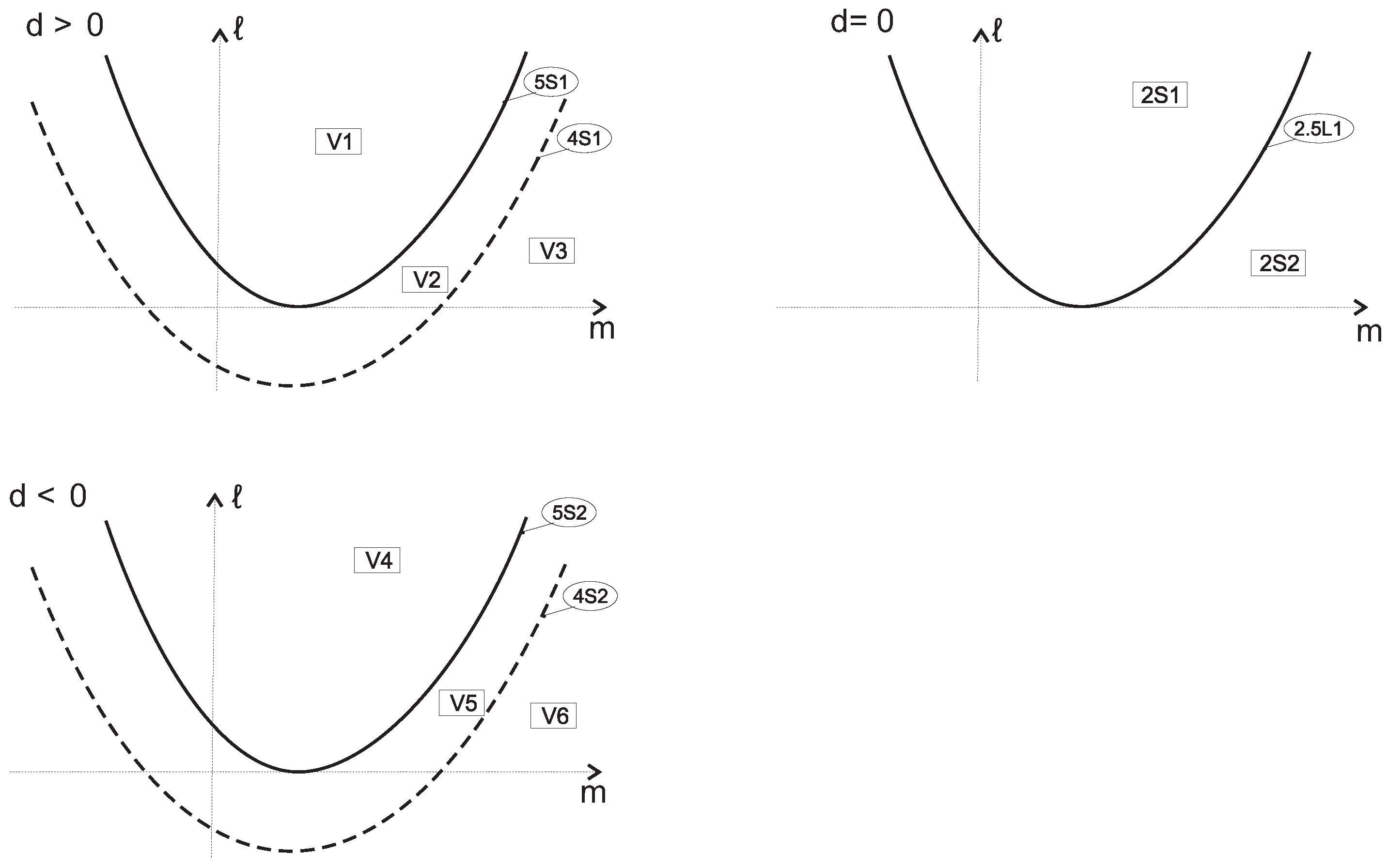
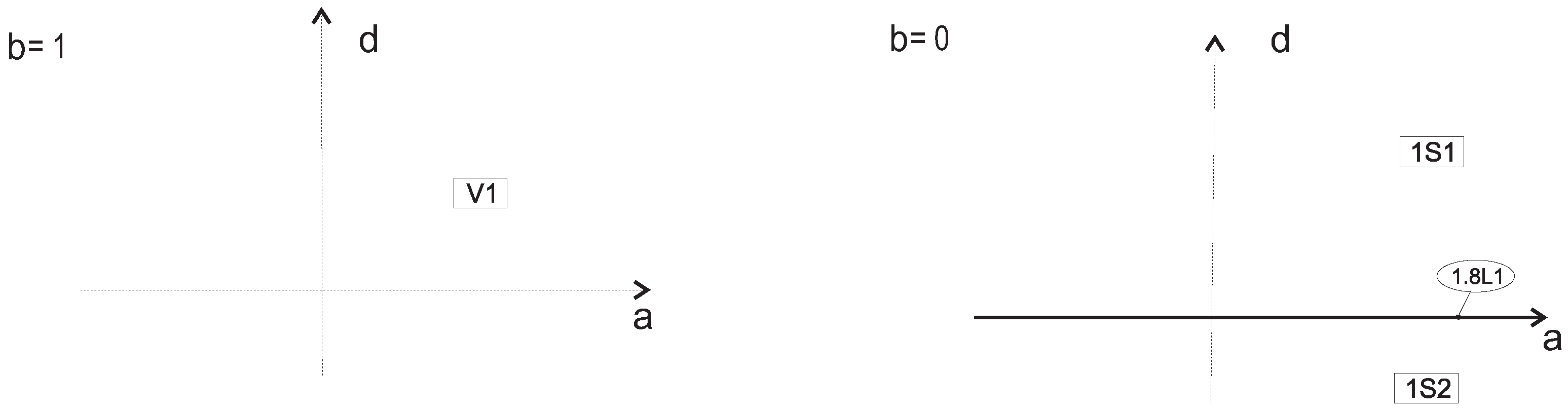
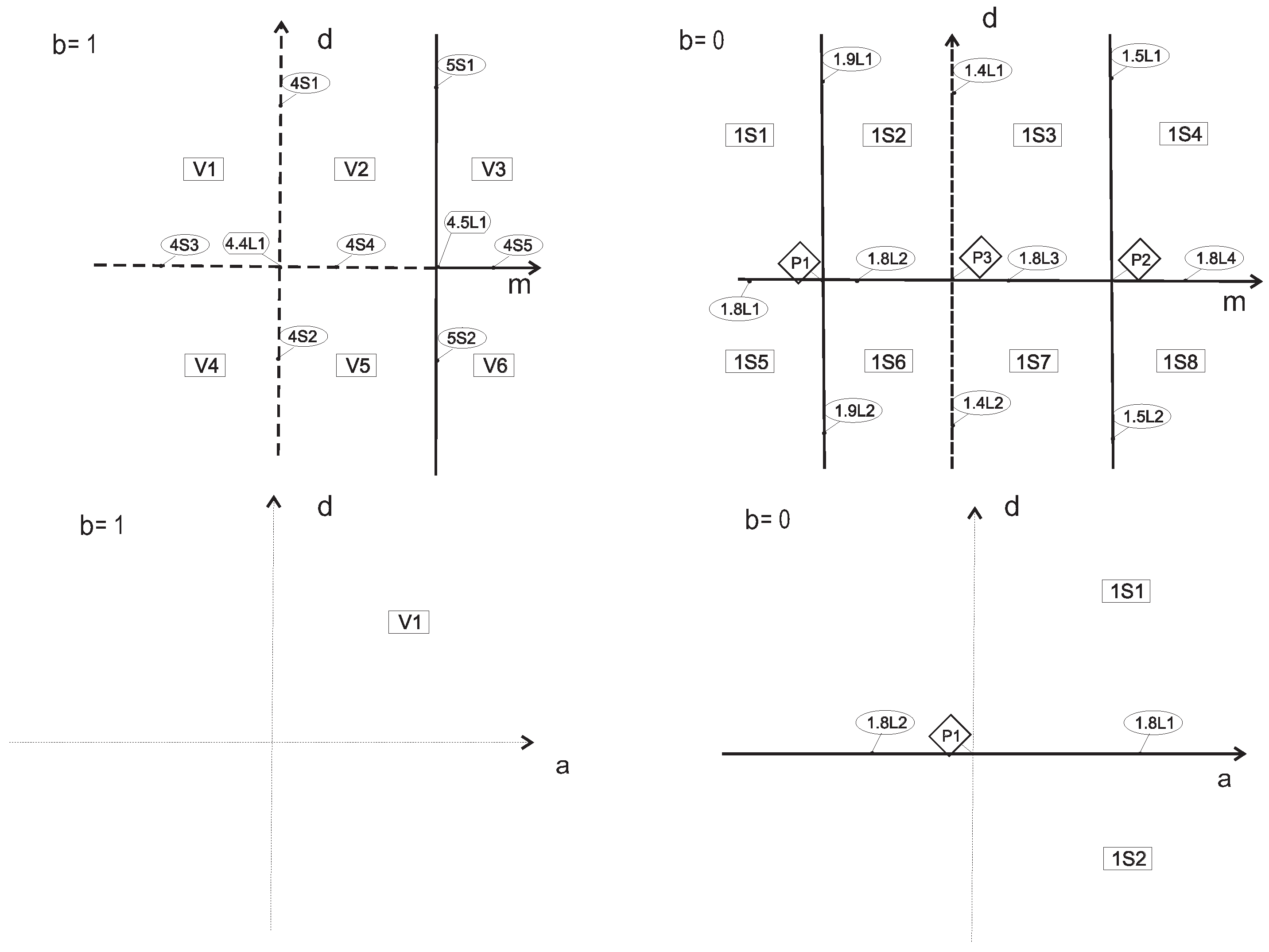
2.3.1. Algebraic Bifurcation Surfaces

The explicit formulas for the bifurcation hypersurfaces of the finite and infinite equilibria of the quadratic systems are given in Reference [4]. These hypersurfaces of bifurcation are algebraic.

(${\mathcal{S}}_1$) The finite equilibria that escape to infinity are controlled by the invariants/comitants ${\mu }_i$ (from $i=0,\dots ,4$). From [4], we obtain the following for family VII:

$${\mu }_0=n^2,{\mu }_1=2bnx,{\mu }_2=(b^2+2dn)x^2,{\mu }_3=2bd{x}^3,{\mu }_4=d^2{x}^4.$$

That is, if $n\ne 0$, no finite equilibria go to infinity. But if $n=0\ne b$ two finite equilibria go to infinity. While if $n=b=0\ne d$, four finite equilibria go to infinity. Finally, if $n=b=d=0$ the system is degenerated, because it has an infinite number of finite equilibria.

For systems VIII we have that

$${\mu }_0={\mu }_1=0,{\mu }_2=ng(x,y),{\mu }_3=bxg(x,y),{\mu }_4=d{x}^{2}g(x,y),$$

where $g(x,y)=\ell x^2+mxy+n{y}^2$. Therefore two finite equilibria go to infinity for every system in family VIII. If $n=0\ne b$, a third finite equilibrium goes to infinity. If $n=b=0\ne d$ then all finite equilibria go to infinity, and if $n=b=d=0$ the system is degenerate.

(${\mathcal{S}}_2$) In this way we denote the bifurcation hypersurface controlling the multiplicity of the finite equilibria. The invariant and comitants needed for family VII are:

$$\mathbf{D}=\mathbf{T}=0;\mathbf{U}=-8d^{3}n{x}^6;\mathbf{P}={(b^2-4dn)}^2{x}^4;\mathrm{R}=4n^2(b^2-4dn)x^2.$$

Using Diagram 6.1 in [4], we can see that if $n\ne 0$ and if $b^2-4dn<0$, the system has two real double finite equilibria. If $b^2-4dn>0$, the system has two complex double finite equilibria. If $b^2-4dn=0$, the system has a finite equilibrium of the multiplicity four.

For family VIII, we only need the comitant $\mathrm{U}=(b^2-4dn)x^2{(\ell x^2+mxy+n{y}^2)}^2$ and ${\mu }_i$. Geometrically, (see Diagram 6.1 in [4]) we can observe that if $n\ne 0$ and $b^2-4dn>0$, the system has two simple real finite equilibria. If $b^2-4dn<0$, the system has two simple complex finite equilibria. If $b^2-4dn=0$ the system has a double finite equilibrium. However, if $n=0\ne b$ we have a single finite real equilibrium, and the rest of the cases are considered in the previous paragraph.

(${\mathcal{S}}_3$) This bifurcation hypersurface is defined by the points in the parameter space for which the system has a weak equilibrium; this can be either a weak focus or a weak saddle. However, for families VII and VIII there is never a weak focus because there are no foci. The reason for this is that both families have an invariant straight line $x=0$ and all their finite equilibria are in that line. Therefore, the existence of foci is not possible. Since foci are not possible, it is not possible to have loops, because, in quadratic systems inside a loop or a limit cycle, must be a focus or a center; see [1]. Therefore, even though weak saddles may exist, they will never form a loop and they will never be topologically relevant. Hence, we may skip surface $S_3$ in this study.

(${\mathcal{S}}_5$) This is the bifurcation hypersurface due to the multiplicity of infinite equilibria, which contains the values for which at least two infinite equilibrium points coalesce. This phenomenon is detected using the invariant polynomial $\eta$ (see Lemma 5.5 in [4]) that, for family VII, is $\eta =-n^2(4\ell n-{(1-m)}^2)$. We will also need the comitants $\tilde{M}=-8({(1-m)}^2{x}^2-3\ell n{x}^2-nxy+mnxy+n^2{y}^2)$ and $C_2=-x(\ell x^2+(m-1)xy+n{y}^2)$.

If $\eta =0\ne n$, then $\tilde{M}\ne 0$ and we have a double infinite equilibrium. If $n=0$ and $m\ne 1$, we also have a double infinite equilibrium. If $n=m-1=0\ne \ell$, we have a triple infinite equilibrium, and if $n=m-1=\ell =0$, the infinite line is filled with equilibria.

For family VIII, we have $\eta =n^2(m^2-4\ell n)$, $\tilde{M}=-8(m^2{x}^2-3\ell n{x}^2+mnxy+n^2{y}^2)$ and $C_2=-x(\ell x^2+mxy+n{y}^2)$. If $\eta =0\ne n$, then $\tilde{M}\ne 0$ and we have a double infinite equilibrium. If $n=0\ne m$, we also have a double infinite equilibrium. If $n=m=0$ (forcing $\ell \ne 0$ to avoid a linear system), we have a triple infinite equilibrium, so we cannot have the infinite line filled with equilibria.

(${\mathcal{S}}_4$) This hypersurface is defined by the points on the parameter space where the system has invariant straight lines. These lines may or may not contain separatrix connections of some equilibria. This hypersurface controls the bifurcation when either invariant straight line is a separatrix connection, or forms a simple $C^{\infty }$ bifurcation when the invariant straight line is not a separatrix connection. This bifurcation is not generally related to the equilbria. This hypersurface is used in Schlomiuk and Vulpe’s papers [11,12,13,14,15,16], where quadratic systems with invariant straight lines are analyzed. More precisely, the authors of those papers used three invariants: $B_1$, $B_2$, and $B_3$. Invariant $B_1=0$ provides a necessary condition for a quadratic system to have an invariant straight line. When $B_1=0$, then $B_2=0$, which provides the necessary and sufficient conditions for a quadratic system to have either non-parallel invariant straight lines or a straight line that collides with infinity. This occurs in families VII and VIII, where $B_1=0$. The values of $B_2$ in both families are very large, and we computed invariant $B_2$ for the distinct normal forms that we created in order to reduce the number of parameters.

2.3.2. Non-Algebraic Bifurcation Hypersurfaces

In most previous research papers on bifurcation diagrams, some non-algebraic bifurcations surfaces were detected. Most times, they are linked to the fact that there is a weak focus somewhere or regions with limit cycles; thus, bifurcation points with a graphic are needed to provide a place of death for the limit cycles. Therefore, these bifurcation surfaces are normally located with the help of continuous arguments and numerical tools. However, our two families have neither focus nor center, and consequently there are no limit cycles. Moreover, we will check that no extra bifurcation surface is needed in order to complete the coherence of the bifurcation diagram.

2.3.3. Differences from Previous Works Using the Same Technique

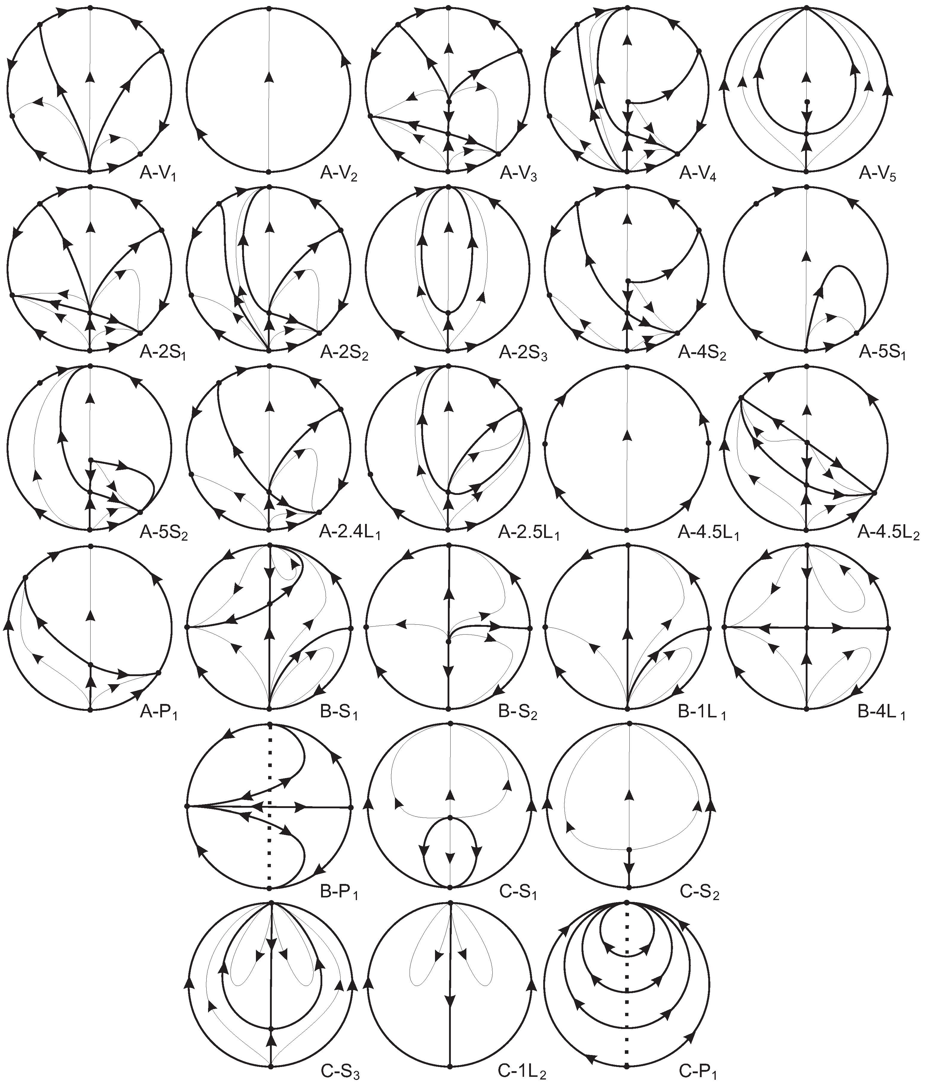
The study of the parameter space in this paper differs from that of previous papers (see, for instance, [10]). In the discussed papers, the parameter spaces usually have five parameters; we studied the possibility of compacting the parameter space into the projective space $\mathbb{R}{\mathbb{P}}^3$ (except in one case, where we had to work in $\mathbb{R}{\mathbb{P}}^4$). The point is that in all these previous works, all the parameters affected only the quadratic part of the system, allowing for a time change that transformed points in ${\mathbb{R}}^4$ into classes of equivalence in $\mathbb{R}{\mathbb{P}}^3$. However, here we cannot carry out this compactification because all parameters are coefficients of the second differential equation, and this does not allow for such a compactification.

We divide the parameter space of dimension three into two-dimensional slices in a similar manner to in the discussed papers, but these slices only depend of the affine part of the parameter space. Here, there is no “slice” for the infinite part, as was the case in the mentioned works.

The bifurcations due to a topological change are indicated with a continuous line, and the ones due to a geometrical change are indicated with a dashed line.

In the three-dimensional parameter space, the regions in the bifurcation diagram with volume are denoted by $V_i$, where i is a number that allows one to distinguish among them. Two-dimensional regions in the bifurcation diagram are denoted $k{S}_i$, where the number k distinguishs the bifurcation surfaces. One-dimensional regions or curves in the bifurcation diagram are denoted by $k.j{L}_i$, where numbers k and j denote the two bifurcation surfaces whose intersection provides the curve being considered. When a curve is the intersection of more than two surfaces, we choose the two with more geometric meaning. Zero-dimensional regions or points in the bifurcation diagram are denoted by $P_i$, where i is a number.

3. Phase Portraits

3.1. Phase Portraits of Systems VII(A)

First, we consider systems (2) with $n=1$, and consequently with $b=0$, i.e., systems (5). Additionally, we split the parameter space $(d,\ell ,m)$ into slices with distinct values of parameter d. After this, we compute the bifurcations in such slices. For systems $VII\left(A1\right)$, the invariants are as follows:

$$\begin{array}{c}\eta =-4\ell +{(m-1)}^2,\mathbf{D}=0,\mathbf{P}=16d^2{x}^4,\mathbf{R}=-16d{x}^2,\\ B_2=-648x^4(16d^2{\ell }^2-8d^2\ell m^2+16d^2\ell m+d^2{m}^4-4d^2{m}^3+\\ 4d^2{m}^2-8d\ell +2d{m}^2-4dm+4d+1).\end{array}$$

It is clear that the slice $d=0$ will be a special slice, since $\mathbf{PR}=0$, and we also see that, for $d=-1$, $B_2=-648\eta (3+4\ell +2m-m^2)x^4$. Moreover, $B_2{|}_{d=0}=-648x^4$, so no point in this slice belongs to $B_2=0$. There are no other intersections between the bifurcation surfaces, and the singular slices are $d=0$ and $d=-1$. We may take $d=1$, $d=-1/2$, and $d=-2$ as generic slices. For these slices, we assign a name to each part and produce their corresponding phase portraits. The two-dimensional regions on slice $d=0$ receive special names because all of slice $d=0$ belongs to surface $S_2$; that is, the double complex finite equilibria that we have on slices $d>0$ coalesce, producing a quadruple equilibrium, which later on splits into two real double equilibria for $d<0$. However the two-dimensional regions for slice $d=-1$ receive the same names as those in slices $d=-1/2$ and $d=-2$, because there is no topological effect on them. Moreover, region $V_4$ disappears when $5S_2$ and $4S_1$ coincide in $d=-1$, but when they split again for $d<-1$, the new region $V_7$ has a different phase portrait (see Figure 3).

The systems when $n=1$ and $a=b=0$ are systems $VII\left(A2\right)$. For these systems, the invariant $\eta$ is the same as before, and $B_2$ can be written as follows:

$$\begin{array}{c}{B}_2=-648d^2{x}^4\left(16L^2-8L{m}^2+16Lm+m^4-4m^3+4m^2\right).\end{array}$$

(14)

Therefore, there is a unique singular slice $d=0$ and we may take two regular slices $d=1$ and $d=-1$ at a volume $(d,\ell ,m)$ (see Figure 4).

3.2. Phase Portraits of Systems VII(B)

Working as for the differential systems with $n=0$, i.e., systems VII(B) (Equations (6) and (7)). For the first case ($m\ne 0$), the three-dimensional space of parameters is $(b,d,m)$ and we slice it along the b-axis. The invariants are as follows:

$$\begin{array}{c}\eta =B_2=\mathbf{D}={\mu }_0={\mu }_1=0,{\mu }_2=b^2{x}^2,{\mu }_3=2bd{x}^3,{\mu }_4=d^2{x}^4,\\ \tilde{M}=-8{(m-1)}^2{x}^2,B_3=3m(b^2-dm+d{m}^2)x^4,\tilde{R}=8(m+1)x^2.\end{array}$$

(15)

Moreover, the change $(x,y,t)\to (-x,-y,-t)$ moves $(b,d,m)\to (-b,d,m)$, so we only need to study the values $b\ge 0$ and we only need the singular slice $b=0$ and a regular slice that may be taken $b=1$; see Figure 5. Since the change is independent of m, the symmetry also exists for the case $m=0$. Thus, when $b=0$, two more finite equilibria escape to infinity, and moreover, when $d=0$, the system becomes degenerated; that is, there is a common factor between the polynomials that define the system. We use ${\mathcal{S}}_8$ to denote the surface when $d=0$. It is also interesting to note the relevance, in this case, of comitant $\tilde{R}$, which only appears in quite degenerate systems and can distinguish between several intricate infinite equilibria with more or fewer sectors; thus, the bifurcation defined by $m=-1$, which we denoted as ${\mathcal{S}}_9$, becomes important inside slice $b=0$.

When $n=m=0$ many invariants and comitants are zero, the relevant comitants obtained with the help of ([4], given in Appendix 2) are ${\mu }_2=b^2{x}^2$ and ${\mu }_4=d^2{x}^4$; see Figure 6.

3.3. Phase Portraits of Systems VII(C) and VII(D)

In a similar way to the differential systems with $n=\ell =0$, i.e., systems (8) and (9), for systems (C) ($m\ne 0$), the three-dimensional space of parameters is $(b,d,m)$ and we take the slices along the b-axis. The invariants are as follows:

$$\begin{array}{c}\eta =B_2=\mathbf{D}={\mu }_0={\mu }_1=0,{\mu }_2=b^2{x}^2,{\mu }_3=2bd{x}^3,{\mu }_4=d^2{x}^4,\\ \tilde{M}=-8{(m-1)}^2{x}^2,C_2=(1-m)x^y,\\ B_3=12dm(m-1)x^4,\tilde{R}=8(m+1)x^2.\end{array}$$

Moreover, the change $(x,y,t)\to (-x,-y,-t)$ moves $(b,d,m)\to (-b,d,m)$, so we only need to study values $b\ge 0$ and we only need singular slice $b=0$ and a regular slice that we take to be $b=1$; see Figure 7. Since the change is independent of m, the symmetry also exists for case $m=0$. Notice that, for $m=1$, $\tilde{M}=C_2=0$, and then the infinite line is filled with equilibria. Moreover, when $b=0$, two more finite equilibria escape to infinity, and when ${\mathcal{S}}_8:d=0$, the system becomes degenerated; that is, there is a common factor between the polynomials that define the system. Also, comitant $\tilde{R}$ is relevant in this family when $b=0$, and thus bifurcation ${\mathcal{S}}_9:m=-1$ needs to be studied.

The systems (D) appear when $m=0$. We have the following values:

$$\begin{array}{c}\eta =B_2=\mathbf{D}={\mu }_0={\mu }_1=0,{\mu }_2=b^2{x}^2,{\mu }_3=2bd{x}^3,{\mu }_4=d^2{x}^4,\\ \tilde{M}=-8x^2,\mathbf{P}=b^4{x}^4,B_3=0.\end{array}$$

Here, we again need only two slices, which are now $b=1$ and $b=0$ in the space $(b,d,a)$. When $b=0$, $d=0$ is also a bifurcation because the systems become degenerated. When $d=a=0$, there is a bifurcation; see Figure 7.

3.4. Phase Portraits of Systems VIII(A)

In our search for the phase portraits of systems (3), we start with the normal form (10), which has three parameters: $(d,b,\ell )$. For these systems, we compute the relevant invariants which are as follows:

$$\begin{array}{c}{B}_1={\mu }_0={\mu }_1=0,{\mu }_2=\ell x^{2}xy+y^2,\\ \eta =1-4\ell ,\mathbf{D}=48(1+b^2-4d)(4\ell -1),\\ B_2=162x^4\left(32b^{2}d{\ell }^2-4b^4{\ell }^2-8b^{2}d\ell -4b^2\ell +b^2-64d^2{\ell }^2+32d^2\ell -4d^2\right).\end{array}$$

(16)

Moreover, we already know that there is symmetry with respect to plane $b=0$, which implies that $b=0$ is a singular slice. For every b, surface $\eta =0$ is a vertical straight line in $(\ell ,d)$, and surface $\mathbf{D}=0$ is formed by two straight lines (one of them coinciding with $\eta =0$). Finally, we detect that for $(d,\ell )=((b^2+1)/4,(1-b^2)/4)$, there is a tangency between D and $B_2$ for every b. There are no other intersections among the surfaces in $b>0$. So, we only need one generic slice, which we take as $b=1$; see Figure 8. Notice that $B_2=0$ splits into three parts and only one of them ($4S_2$) is topologically relevant.

3.5. Phase Portraits of Systems VIII(B)

The systems with $n=0$, $m=1$ $a=0$ and $\ell =0$ form two-parameter systems (11). The relevant invariants are as follows:

$$\begin{array}{c}{\mu }_0={\mu }_1={\mu }_2=\eta =\kappa =\tilde{K}=\tilde{L}={\kappa }_1=B_1=B_2=0,\\ {\mu }_3=b{x}^{2}y,{\mu }_4=d{x}^{3}y,\tilde{M}=-8x^3,K_1=x^{2}y,B_3=3d{x}^4.\end{array}$$

(17)

Therefore, the only bifurcation curves are $d=0$ and $b=0$, and we have Figure 9 (left).

3.6. Phase Portraits of Systems VIII(C)

The systems with $n=m=0$, $a=\ell =1$ are the two-parameter systems (13). The relevant invariants are as follows:

$$\begin{array}{c}{\mu }_0={\mu }_1={\mu }_2=\eta =\kappa =\tilde{M}=\tilde{K}={\kappa }_1=B_1=B_2=B_3=0,\\ {\mu }_3=b{x}^3,{\mu }_4=d{x}^4,C_2=-x^3,K_1=x^3,K_3=6(2-b)b{x}^6.\end{array}$$

(18)

Therefore, the only bifurcation curves are $b=0$ and $b=2$, and inside $b=0$, point $d=0$ is also relevant. For $b=0$, another finite equilibrium point goes to infinity and thus belongs to surface ${\mathcal{S}}_1$. When $b=2$, there is a bifurcation related to the local sectors of the intricate infinite equilibrium point, and we denote this as line $8L_1$. These are shown in Figure 9 (right).

4. Global Geometrical Properties of Family VII

The Classification Theorem

Topologically equivalent phase portraits can appear in different regions of the bifurcation diagram inside the parameter space. For family VII, the bifurcation diagram has 106 different regions. In order to distinguish the distinct phase portraits, we use invariants; more precisely, we use integer-valued invariants. Such invariants were previously used in [7].

Definition 1. 

$I_1\left(S\right)$ denotes a code defined in [17] that provides the number and the local phase portraits of all the finite and infinite equilibria of the differential system. For instance, $I_1\left(S\right)=12$ indicates that the differential system has only one infinite node and has no real finite equilibria, and $I_1\left(S\right)=144$ indicates that the differential system has a finite saddle-node, an infinite intricate equillibrium with one parabolic and one hyperbolic sector in both sides of the line infinity and an infinite node, or $I_1\left(S\right)=195$ indicates that the differential system has an infinite amount of finite equilibria on a straight line, and these are all the finite equilibria—additionally, it has an infinite node. Consequently, two differential systems with a distinct code $I_1\left(S\right)$ can never be topologically equivalent.

Definition 2. 

$I_2\left(S\right)$ denotes a code defined by a sequence of digits (varying from 0 to 4); each digit provides the number of separatrices non-contained at infinity that end (or start) at an infinite equilibrium point. In each sequence, the number of digits is 2, 4, or 6 as a function of the number of infinite equilibria. The sequence can start at an arbitrary infinite equilibria but all sequences must be listed in a particular specific order, either clockwise or counterclockwise, along the line of infinity to produce the biggest possible number.

Since the local phase portraits of nodes and foci are topologically equivalent, we do not distinguish between them. Of course, they can be distinguished inside the $C^1$ class.

Definition 3. 

$I_3\left(S\right)$ denotes a code defined by a sequence of digits (varying from 0 to 4); each digit provides the number of separatrices non-contained at infinity that end (or start) at an infinite equilibrium point. In each sequence, the number of digits is 2, 4, or 6 as a function of the number of infinite equilibria. The sequence can start at an arbitrary infinite equilibria but all sequences must be listed in a particular specific order, either clockwise or counterclockwise, along the line of infinity to produce the biggest possible number.

Lemma 1. 

Let S be a system belonging to family VII. Then, the 106 different parts in which the bifurcation diagram splits (obtained in Section 3.1, Section 3.2 and Section 3.3) may be condensed by taking one representative of each set of the topologically different phase portraits, totaling 33 cases, as shown in the next diagram and

Table 1. Topological equivalences.

Presented Phase Portrait	Multiple Equilibrium	Invariant Straight Line	Other Reasons
$A1\text{-}{V}_1$	$B1\text{-}1.5L_1$		$A2\text{-}{V}_1$
$A1\text{-}{V}_2$		$A_2\text{-}4S_1$	$A2\text{-}{V}_2,A2\text{-}{V}_3$
$A1\text{-}{V}_3$			$A2\text{-}{V}_4$
$A1\text{-}{V}_4$
$A1\text{-}{V}_5$		$A2\text{-}4S_2$	$A1\text{-}{V}_6,A1\text{-}{V}_7,A2\text{-}{V}_5,A2\text{-}{V}_6$
$A1\text{-}2S_1$
$A1\text{-}2S_2$
$A1\text{-}4S_1$
$A1\text{-}5S_1$			$A2\text{-}5S_1$
$A1\text{-}5S_2$
$A1\text{-}5S_3$			$A2\text{-}5S_2$
$A1\text{-}2.5L_1$
$A1\text{-}4.5L_1$
$A2\text{-}2S_1$
$A2\text{-}2S_2$
$A2\text{-}2.5L_1$
$B1\text{-}{V}_1$		$B1\text{-}4S_1,B1\text{-}4S_2,B1\text{-}4S_3$	$B1\text{-}{V}_2$, $B1\text{-}{V}_3$, $B1\text{-}{V}_5$, $B2\text{-}{V}_1$
		$C\text{-}4S_1$, $C\text{-}4S_2$, $C\text{-}4S_3$	$C\text{-}{V}_1$, $C\text{-}{V}_2$, $C\text{-}{V}_4$, $C\text{-}{V}_5$
		$C\text{-}4S_4$, $C\text{-}4.4L_1$	$D\text{-}{V}_1$
$B1\text{-}{V}_4$			$B1\text{-}{V}_6$, $C\text{-}{V}_3$, $C\text{-}{V}_6$
$B1\text{-}1S_1$			$B1\text{-}1S_5$, $C\text{-}1S_1$, $C\text{-}1S_5$
$B1\text{-}1S_2$	$B1\text{-}1.9L_1$, $B1\text{-}1.9L_2$	$B1\text{-}1.4L_1$, $B1\text{-}1.4L_2$	$B1\text{-}1S_3$, $B1\text{-}1S_6$, $B1\text{-}1S_7$
			$B2\text{-}1S_1$, $B2\text{-}1S_2$, $C\text{-}1S_2$
	$C\text{-}1.9L_1$, $C\text{-}1.9L_2$	$C\text{-}1.4L_1$,$C\text{-}1.4L_2$,	$C\text{-}1S_3$, $C\text{-}1S_6$, $C\text{-}1S_7$
			$D\text{-}1S_1$, $D\text{-}1S_2$
$B1\text{-}1S_4$			$B1\text{-}1S_8$, $C\text{-}1S_4$, $C\text{-}1S_8$
$B1\text{-}4S_3$		$C\text{-}4S_5$
$B1\text{-}5S_1$
$B1\text{-}1.5L_2$
$B1\text{-}1.8L_1$	$B1\text{-}{P}_1$		$B1\text{-}1.8L_2$, $B1\text{-}1.8L_4$
	$C\text{-}{P}_1$		$C\text{-}1.8L_1$, $C\text{-}1.8L_2$
$B1\text{-}1.8L_3$	$B1\text{-}{P}_2$
$B1\text{-}{P}_3$			$C\text{-}{P}_3$, $D\text{-}{P}_1$
$B2\text{-}1.8L_1$			$D\text{-}1.8L_1$, $D\text{-}1.8L_2$
$C\text{-}5S_1$		$C\text{-}4.5L_1$	$C\text{-}5S_2$
$C\text{-}1.5L_1$			$C\text{-}1.5L_2$
$C\text{-}1.8L_3$
$C\text{-}1.8L_4$
$C\text{-}{P}_2$

, with the help of the invariant $\mathcal{I}=(I_1,I_3)$.

$$I_1=\left\{\begin{array}{c}12\left(A1\text{-}{V}_1\right)\hfill \\ 13\left(A1\text{-}{V}_2\right)\hfill \\ 14\&I_3=\left\{\begin{array}{c}1010\left(B1\text{-}1S_2\right)\hfill \\ 1111\left(A1\text{-}5S_1\right)\hfill \end{array}\right.\hfill \\ 44\left(A1\text{-}2S_1\right)\hfill \\ 45\left(A1\text{-}2S_2\right)\hfill \\ 46\left(A1\text{-}2.5L_1\right)\hfill \\ 47\left(A2\text{-}2S_1\right)\hfill \\ 50\left(A1\text{-}{V}_3\right)\hfill \\ 51\&I_3=\left\{\begin{array}{c}111110\left(A1\text{-}4S_1\right)\hfill \\ 111111\left(A1\text{-}{V}_5\right)\hfill \\ 211210\left(A1\text{-}{V}_4\right)\hfill \end{array}\right.\hfill \\ 52\&I_3=\left\{\begin{array}{c}2111\left(A1\text{-}4.5L_1\right)\hfill \\ 2121\left(A1\text{-}5S_3\right)\hfill \\ 2221\left(A1\text{-}5S_2\right)\hfill \end{array}\right.\hfill \\ 71\left(A2\text{-}2S_2\right)\hfill \\ 72\left(A2\text{-}2.5L_1\right)\hfill \\ 138\left(B1\text{-}1S_4\right)\hfill \\ 144\left(B1\text{-}{V}_1\right)\hfill \\ 145\&I_3=\left\{\begin{array}{c}1111\left(B1\text{-}4S_3\right)\hfill \\ 2121\left(B1\text{-}{V}_4\right)\hfill \end{array}\right.\hfill \\ 146\left(B1\text{-}5S_1\right)\hfill \\ 147\left(C\text{-}5S_1\right)\hfill \\ 164\left(B1\text{-}1S_1\right)\hfill \\ 167\left(B1\text{-}1.5L_2\right)\hfill \\ 170\left(C\text{-}1.5L_1\right)\hfill \\ 186\left(B1\text{-}1.8L_1\right)\hfill \\ 188\left(C\text{-}1.8L_4\right)\hfill \\ 190\left(C\text{-}1.8L_3\right)\hfill \\ 195\left(B2\text{-}1.8L_1\right)\hfill \\ 196\left(B1\text{-}{P}_3\right)\hfill \\ 202\left(B1\text{-}1.8L_3\right)\hfill \\ 208\left(C\text{-}{P}_2\right)\hfill \end{array}\right.$$

Here, we describe each of the configurations of equilibria that appear in the previous diagram and also in the diagram presented in Section 5. The notation of the simple equilibria is quite obvious. The reader is advised to obtain the complete notation from ([4], Section 3.7); see also ([4], Appendix A).

• (12) $\varnothing ;N$;
• (13) $\varnothing ;S,N,N$;
• (14) $\varnothing ;\left({\displaystyle \genfrac{}{}{0pt}{}{0}{2}}\right)SN,N$;
• (23) $s,a;N$;
• (44) $sn;N$;
• (45) $sn;S,N,N$;
• (46) $sn;\left({\displaystyle \genfrac{}{}{0pt}{}{0}{2}}\right)SN,N$;
• (47) $cp;N$;
• (50) $sn,sn;N$;
• (51) $sn,sn;S,N,N$;
• (52) $sn,sn;\left({\displaystyle \genfrac{}{}{0pt}{}{0}{2}}\right)SN,N$;
• (71) $phph;S,N,N$;
• (72) $phph;\left({\displaystyle \genfrac{}{}{0pt}{}{0}{2}}\right)SN,N$;
• (84) $a;\left({\displaystyle \genfrac{}{}{0pt}{}{1}{1}}\right)SN$;
• (124) $s,a;\left({\displaystyle \genfrac{}{}{0pt}{}{2}{2}}\right)PH-PH,N$;
• (134) $s,a;\left({\displaystyle \genfrac{}{}{0pt}{}{1}{1}}\right)SN,\left({\displaystyle \genfrac{}{}{0pt}{}{1}{1}}\right)NS,N$;
• (135) $s,a;\left({\displaystyle \genfrac{}{}{0pt}{}{2}{2}}\right)PH-H,N$;
• (137) $\varnothing ;\left({\displaystyle \genfrac{}{}{0pt}{}{2}{2}}\right)H-H,N$;
• (138) $\varnothing ;\left({\displaystyle \genfrac{}{}{0pt}{}{2}{2}}\right)E-E,S$;
• (141) $\varnothing ;\left({\displaystyle \genfrac{}{}{0pt}{}{1}{1}}\right)SN,\left({\displaystyle \genfrac{}{}{0pt}{}{1}{1}}\right)NS,N$.
• (142) $\varnothing ;\left({\displaystyle \genfrac{}{}{0pt}{}{2}{2}}\right)PH-H,N$;
• (144) $sn;\left({\displaystyle \genfrac{}{}{0pt}{}{2}{2}}\right)PH-PH,N$;
• (145) $sn;\left({\displaystyle \genfrac{}{}{0pt}{}{2}{2}}\right)E-E,S$;
• (146) $sn;\left({\displaystyle \genfrac{}{}{0pt}{}{2}{3}}\right)HE-P$;
• (147) $sn;[\infty ;N]$;
• (149) $sn;\left({\displaystyle \genfrac{}{}{0pt}{}{1}{1}}\right)SN,\left({\displaystyle \genfrac{}{}{0pt}{}{1}{1}}\right)NS,N$.
• (152) $sn;\left({\displaystyle \genfrac{}{}{0pt}{}{2}{2}}\right)PH-H,N$;
• (153) $cp;\left({\displaystyle \genfrac{}{}{0pt}{}{2}{2}}\right)PH-H,N$;
• (160) $s;\left({\displaystyle \genfrac{}{}{0pt}{}{2}{2}}\right)E-E,\left({\displaystyle \genfrac{}{}{0pt}{}{1}{1}}\right)SN$;
• (161) $a;\left({\displaystyle \genfrac{}{}{0pt}{}{2}{2}}\right)PH-PH,\left({\displaystyle \genfrac{}{}{0pt}{}{1}{1}}\right)SN$;
• (162) $s;\left({\displaystyle \genfrac{}{}{0pt}{}{3}{3}}\right)EE-P$;
• (163) $a;\left({\displaystyle \genfrac{}{}{0pt}{}{3}{3}}\right)HPH-P$;
• (164) $\varnothing ;\left({\displaystyle \genfrac{}{}{0pt}{}{4}{2}}\right)PHP-PHP,N$;
• (166) $\varnothing ;\left({\displaystyle \genfrac{}{}{0pt}{}{3}{2}}\right)E-PH,\left({\displaystyle \genfrac{}{}{0pt}{}{1}{1}}\right)SN$;
• (167) $\varnothing ;\left({\displaystyle \genfrac{}{}{0pt}{}{4}{3}}\right)EH-HE$;
• (168) $\varnothing ;\left({\displaystyle \genfrac{}{}{0pt}{}{4}{3}}\right)EE-HH$;
• (170) $a;[\infty ;\left({\displaystyle \genfrac{}{}{0pt}{}{3}{0}}\right)ES]$;
• (186) $\left(\ominus [|];s\right);(\ominus [|];N_2^f),N$;
• (188) $\left(\ominus [|];n\right);(\ominus [|];N_2^{\infty }),S$;
• (190) $\left(\ominus [|];n\right);(\ominus [|];S_2),N$;
• (195) $\left(\ominus [|];\varnothing \right);\left(\ominus [|];\left({\displaystyle \genfrac{}{}{0pt}{}{1}{1}}\right)S{N}_2\right),N$;
• (196) $\left(\ominus [{|}^{\mathbf{2}}];\varnothing \right);(\ominus [{|}^2];\varnothing ),N$;
• (198) $\left(\ominus [|];\varnothing \right);(\ominus [|];N),\left({\displaystyle \genfrac{}{}{0pt}{}{1}{1}}\right)SN$;
• (202) $\left(\ominus [|];n^d\right);\left(\ominus [|];\left({\displaystyle \genfrac{}{}{0pt}{}{0}{2}}\right)S{N}_2\right)$,
• (203) $\left(\ominus [|];\varnothing \right);\left(\ominus [|];\left({\displaystyle \genfrac{}{}{0pt}{}{1}{2}}\right)E-H\right)$;
• (208) $\left(\ominus [|];n^{*}\right);\left[\infty ;\left(\ominus [|];{\varnothing }_2\right)\right]$.

5. Global Geometrical Properties of Family VIII

The Classification Theorem

We are going to proceed in the same way as in the previous section for family VIII. The invariants that we will need are exactly the same $\mathcal{I}=(I_1,I_3)$ as the ones we have already defined.

Lemma 2. 

Let S be a system belonging to family VIII. Then, the 37 different parts in which the bifurcation diagram splits (obtained in Section 3.4 and Section 3.5) may be condensed by taking one representative of each set of topologically different phase portraits, totaling 26 cases, as shown in the next diagram and

Table 2. Topological equivalences.

Presented Phase Portrait	Multiple Equilibrium	Invariant Straight Line	Other Reasons
$A\text{-}{V}_1$
$A\text{-}{V}_2$	$C\text{-}1L_1$
$A\text{-}{V}_3$		$A\text{-}4S_1$, $A\text{-}4S_3$, $A\text{-}4.4L_1$	$A\text{-}{V}_6$, $A\text{-}{V}_7$,
$A\text{-}{V}_4$
$A\text{-}{V}_5$		$A\text{-}4.4L_2$
$A\text{-}2S_1$
$A\text{-}2S_2$
$A\text{-}2S_3$
$A\text{-}4S_2$
$A\text{-}5S_1$
$A\text{-}5S_2$
$A\text{-}2.4L_1$
$A\text{-}2.5L_1$
$A\text{-}4.5L_1$
$A\text{-}4.5L_2$	$P_2$		$A\text{-}4.5L_3$
$A\text{-}{P}_1$
$B\text{-}{S}_1$
$B\text{-}{S}_2$		$B\text{-}4L_2$
$B\text{-}1L_1$
$B\text{-}4L_1$
$B\text{-}{P}_1$
$C\text{-}{S}_1$
$C\text{-}{S}_2$	$C\text{-}8L_1$
$C\text{-}{S}_3$
$C\text{-}1L_2$
$C\text{-}{P}_1$

, with the help of the invariant $\mathcal{I}=(I_1,I_3)$.

$$I_1=\left\{\begin{array}{c}12\left(A\text{-}{V}_2\right)\hfill \\ 23\left(A\text{-}{V}_5\right)\hfill \\ 44\left(A\text{-}2S_3\right)\hfill \\ 84\left(C\text{-}{S}_2\right)\hfill \\ 124\left(A\text{-}4.5L_2\right)\hfill \\ 134\&I_3=\left\{\begin{array}{c}111010\left(A\text{-}4S_2\right)\hfill \\ 111110\left(A\text{-}{V}_3\right)\hfill \\ 211110\left(A\text{-}{V}_4\right)\hfill \end{array}\right.\hfill \\ 135\left(A\text{-}5S_2\right)\hfill \\ 137\left(A\text{-}4.5L_1\right)\hfill \\ 141\left(A\text{-}{V}_1\right)\hfill \\ 142\left(A\text{-}5S_1\right)\hfill \\ 144\left(A\text{-}{P}_1\right)\hfill \\ 149\&I_3=\left\{\begin{array}{c}111010\left(A\text{-}2.4L_1\right)\hfill \\ 111110\left(A\text{-}2S_1\right)\hfill \\ 211110\left(A\text{-}2S_2\right)\hfill \end{array}\right.\hfill \\ 152\left(A\text{-}2.5L_1\right)\hfill \\ 160\&I_3=\left\{\begin{array}{c}1111\left(B\text{-}4L_1\right)\hfill \\ 2121\left(B\text{-}{S}_1\right)\hfill \end{array}\right.\hfill \\ 161\left(B\text{-}{S}_2\right)\hfill \\ 162\left(C\text{-}{S}_3\right)\hfill \\ 163\left(C\text{-}{S}_1\right)\hfill \\ 166\left(B\text{-}1L_1\right)\hfill \\ 168\left(C\text{-}1L_2\right)\hfill \\ 198\left(B\text{-}{P}_1\right)\hfill \\ 203\left(C\text{-}{P}_1\right)\hfill \end{array}\right.$$

6. Conclusions and Comments

In recent decades, different attempts have been made to obtain a complete classification of the phase portraits of quadratic systems. Any serious attempt must cover the following points: (1) it must split the whole set of quadratic systems into subfamilies that are easier to study; (2) it must contain all the realizable phase portraits; (3) either there should be no repetitions among the obtained phase portraits, or there must be an algorithm to detect such repetitions; (4) it must be possible to study all the subfamilies obtained.

Up to now, no attempt has been able to achieve all these conditions. In addition to the different previous attempts, we present the one studied in this paper. At present, 3 families out of 10 have been studied, and we are already working on the study of families V-VI-IX and X, which can feasibly be achieved. However, families I to III are too generic and cannot be reduced to an acceptable number of parameters. In [18], J.W. Reyn compiled several articles by himself and collaborators in which they tried to systematically study all the phase portraits of quadratic systems where j finite singularities have reached infinity. They succeeded for $j=4,3,2$ (with some gaps in $j=2$) but their work on $j=1$ obtained many more gaps and they recognized that $j=0$ was not achievable using their methods. Gasull, Llibre, and others tried a similar approach in a series of papers in which they studied phase portraits with exactly j finite singularities (this was similar to the work of Reyn but not exactly the same). They obtained complete results for $j=0$, while their work on $j=1$ had at least one missed phase portrait, and their work on $j=2$ was only partial (one focus plus one antisaddle).

The most serious attempt for a complete classification of phase portraits comes from the other direction: instead of starting from the most degenerate cases and moving to the most generic, we started from the most generic. Of course, in this case, the goal is not to produce a complete bifurcation diagram, but simply a list of realizable phase portraits. The technique is to first detect all the potential (by a potential phase portrait, we mean a phase portrait which is compatible with the number and type of equilibria that can be obtained in a fixed class of systems, but may not be realizable for other, deeper reasons) and then to look for an example of realization or a proof of its impossibility. Using this technique, Artés and collaborator found all structurally stable phase portraits of quadratic systems (codimension 0), all of codimension 1, and are halfway to obtaining all codimension 2 phase portraits. All the phase portraits obtained using this algorithm lack limit cycles. A second step would be to detect how many limit cycles could be added to each phase portrait without them. Even though this technique does not use bifurcation diagrams, the step of looking for examples relies on the hundreds of papers in the bibliography in which these phase portraits (or similar ones) were found.

In summary, it seems clear that a single line of research cannot provide a complete classification, but the combination of all of them may achieve this. At present, we already have a database which contains more than 1000 phase portraits (without limit cycles) which covers the most degenerated cases and also the most generic, and the only remaining gap is codimensions 2–4, which still needs to be completed.

References

1. Coppel, W.A. A Survey of Quadratic Systems. Differ. Equ. 1966, 2, 293–304. [Google Scholar] [CrossRef]
2. Büchel, W. Zur Topologie der Durch Eine Gewöhnliche Differentialgleichung Erster Ordnung und Ersten Grades Definierten Kurvenschar; Druck von BG Teubner: Leipzig, Germany, 1904; pp. 33–68. [Google Scholar]
3. Chicone, C.; Tian, J. On general properties of quadratic systems. Am. Math. Mon. 1982, 89, 167–178. [Google Scholar] [CrossRef]
4. Artés, J.C.; Llibre, J.; Schlomiuk, D.; Vulpe, N. Geometric Configurations of Singularities of Planar Polynomial Differential Systems. In A Global Classification in the Quadratic Case; Birkhäuser: Basel, Switzerland, 2021. [Google Scholar]
5. Ye, Y. Theory of limit cycles. In Translations of Mathematical Monographs; American Mathematical Society: Providence, RI, USA, 1986; Volume 66. [Google Scholar]
6. Gasull, A.; Li-Ren, S.; Llibre, J. Chordal quadratic systems. Rocky Mt. Math. 1986, 16, 751–782. [Google Scholar] [CrossRef]
7. Artés, J.C.; Cairó, L.; Llibre, J. Phase portraits of the family IV of the quadratic polynomial differential systems. Qual. Theory Dyn. Syst. 2025, 24, 66. [Google Scholar] [CrossRef]
8. Cairó, L.; Llibre, J. Phase portraits of the families VII and VIII of the Quadratic Systems. Axioms 2025, 12, 756. [Google Scholar] [CrossRef]
9. Artés, J.C.; Llibre, J.; Schlomiuk, D.; Vulpe, N. Global analysis of Riccati quadratic differential systems. Int. J. Bifurc. Chaos 2024, 34, 2450004. [Google Scholar] [CrossRef]
10. Artés, J.C.; Llibre, J.; Schlomiuk, D. The geometry of quadratic differential systems with a weak focus of second order. Int. Bifur. Chaos Appl. Sci. Eng. 2006, 16, 3127–3194. [Google Scholar] [CrossRef]
11. Schlomiuk, D.; Vulpe, N. Planar quadratic differential systems with invariant straight lines of at least five total multiplicity. Qual. Theory Dyn. Syst. 2004, 5, 135–194. [Google Scholar] [CrossRef]
12. Schlomiuk, D.; Vulpe, N. Integrals and phase portraits of planar quadratic differential systems with invariant lines of at least five total multiplicity. Rocky Mt. Math. 2008, 38, 2015–2075. [Google Scholar] [CrossRef]
13. Schlomiuk, D.; Vulpe, N. Integrals and phase portraits of planar quadratic differential systems with invariant lines of total multiplicity four. Bul. Acad. Ştiinţe Repub. Mold. Mat. 2008, 56, 27–83. [Google Scholar]
14. Schlomiuk, D.; Vulpe, N. Planar quadratic differential systems with invariant straight lines of total multiplicity four. Nonlinear Anal. 2008, 68, 681–715. [Google Scholar] [CrossRef]
15. Schlomiuk, D.; Vulpe, N. Global classification of the planar Lotka–Volterra differential systems according to their configurations of invariant straight lines. J. Fixed Point Theory Appl. 2010, 8, 177–245. [Google Scholar] [CrossRef]
16. Schlomiuk, D.; Vulpe, N. Global topological classification of Lotka–Volterra quadratic differential systems. Electron. J. Differ. Equ. 2012, 2012, 69. [Google Scholar]
17. Artés, J.C.; Llibre, J.; Schlomiuk, D.; Vulpe, N. Global topological configurations of singularities for the whole family of quadratic differential systems. Qual. Theory Dyn. Syst. 2020, 19, 51. [Google Scholar] [CrossRef]
18. Reyn, J.W. Phase portraits of planar quadratic systems. In Mathematics and Its Applications; Springer: New York, NY, USA, 2007; Volume 583, xvi+334p. [Google Scholar]
Figure 1. Phase portraits for family VII.
Appliedmath 05 00068 g001
Figure 2. Phase portraits for family VIII.
Appliedmath 05 00068 g002
Figure 3. Slices for subfamily V I I ( A 1 ) .
Appliedmath 05 00068 g003
Figure 4. Slices for subfamily V I I ( A 2 ) .
Appliedmath 05 00068 g004
Figure 5. Slices for subfamily V I I ( B 1 ) .
Appliedmath 05 00068 g005
Figure 6. Slices for subfamily V I I ( B 2 ) .
Appliedmath 05 00068 g006
Figure 7. Slices for subfamilies V I I ( C ) (up) and V I I ( D ) (down).
Appliedmath 05 00068 g007
Figure 8. Slices for subfamily V I I I ( A ) .
Appliedmath 05 00068 g008
Figure 9. Bifurcation diagrams for subfamilies V I I I ( B ) (left) and V I I I ( C ) (right).
Appliedmath 05 00068 g009