Stochastic Graph-Based Models of Tumor Growth and Cellular Interactions

Abstract

The tumor microenvironment is a highly dynamic and complex system where cellular interactions evolve over time, influencing tumor growth, immune response, and treatment resistance. In this study, we develop a graph-theoretic framework to model the tumor microenvironment, where nodes represent different cell types, and edges denote their interactions. The temporal evolution of the tumor microenvironment is governed by fundamental biological processes, including proliferation, apoptosis, migration, and angiogenesis, which we model using differential equations with stochastic effects. Specifically, we describe tumor cell population dynamics using a logistic growth model incorporating both apoptosis and random fluctuations. Additionally, we construct a dynamic network to represent cellular interactions, allowing for an analysis of structural changes over time. Through numerical simulations, we investigate how key parameters such as proliferation rates, apoptosis thresholds, and stochastic fluctuations influence tumor progression and network topology. Our findings demonstrate that graph theory provides a powerful mathematical tool to analyze the spatiotemporal evolution of tumors, offering insights into potential therapeutic strategies. This approach has implications for optimizing cancer treatments by targeting critical network structures within the tumor microenvironment.

1. Introduction

Understanding the evolution of cellular populations over time is crucial to comprehending various biological processes, particularly in the context of cancer biology. The tumor microenvironment (TME) plays a pivotal role in shaping the behavior of tumor cells, including their growth, invasion, and response to therapies [1,2]. Traditional models of tumor growth, such as the logistic growth equation, offer a foundational framework for describing how tumor populations expand by considering intrinsic growth limitations [3]. However, the TME is subject to various dynamic and unpredictable factors, such as immune responses, nutrient availability, and the presence of therapeutic interventions [1]. These factors introduce substantial randomness that purely deterministic models fail to capture, making it necessary to use stochastic models to provide a more accurate representation of tumor evolution [4].

This study investigates a stochastic tumor growth model that extends the classical logistic equation by incorporating an additional decay term and stochasticity through a Gaussian white noise process [5]. The model not only accounts for the bounded growth of tumor cells but also introduces mechanisms that describe external pressures from the TME, such as immune attacks, hypoxia, and chemotherapy, which can lead to tumor decline or remission [6]. Furthermore, the stochastic component models the unpredictable variations resulting from the TME’s environmental and therapeutic uncertainties, thus offering a more flexible and realistic description of tumor growth and adaptation [7].

To analyze this stochastic model, we employ numerical approximation techniques, with a focus on the Euler–Maruyama method [8], which is widely used for solving stochastic differential equations (SDEs) in computational cancer modeling. Additionally, we extend our analysis by incorporating a dynamic graph evolution framework, where tumor cells are represented as nodes in a network that evolves over time. This computational approach enables the modeling of complex biological systems through graph theory, with edges representing interactions or communication pathways between cellular components of the TME. Such frameworks are particularly valuable for capturing the multiscale dynamics inherent in cancer biology, including both short-term signaling events and long-term evolutionary adaptations within heterogeneous cell populations [9].

This method captures the changing interactions and relationships within the TME, which is composed not only of tumor cells but also of immune cells, fibroblasts, endothelial cells, and extracellular matrix components [9]. These dynamic interactions are crucial for understanding how signaling pathways evolve during tumor progression, how immune surveillance is evaded, and how resistance to therapies may develop [1]. The TME acts as a constantly shifting landscape where feedback loops between stromal and malignant cells drive tumor adaptation and therapeutic escape. By modeling these interactions as evolving graphs, we can track shifts in communication networks and identify critical transitions in tumor behavior [10,11].

By adopting this graph-based perspective, we can simulate and analyze topological changes in the network—such as shifts in node centrality, clustering coefficients, and path lengths—that reflect underlying biological adaptations [12]. For instance, increased node centrality may indicate a rise in signaling dominance of certain cell types, while altered clustering patterns might suggest new functional groupings among subpopulations of tumor or immune cells. These structural properties provide insights into how tumors adapt to their ever-changing microenvironment, including responses to hypoxia, nutrient deprivation, and therapeutic interventions [13]. For example, hypoxia-induced angiogenesis can lead to reconfiguration of vascular networks, which can be modeled as changes in connectivity and modularity of endothelial nodes.

Moreover, such dynamic modeling helps elucidate how cellular heterogeneity and spatial organization influence treatment outcomes. In particular, alterations in the connectivity of immune cell nodes might indicate immunosuppressive reprogramming, such as the emergence of regulatory T cells or myeloid-derived suppressor cells that disrupt effector immune signaling [14]. Similarly, increased network modularity—a measure of compartmentalization—could signal the formation of distinct tumor subclone clusters that are isolated from immune surveillance or drug delivery [14]. These insights have direct implications for predicting responses to immunotherapy, targeted therapy, and combination treatments, as network topology can serve as a predictive biomarker for therapeutic efficacy [15].

By integrating stochastic modeling with dynamic graph evolution, this work offers a more nuanced and adaptable approach to understanding tumor dynamics. The results provide deeper insights into how tumor populations evolve under uncertainty, interact within a complex microenvironment, and adapt to changing conditions, contributing to a more comprehensive understanding of cancer progression and therapeutic challenges [16].

In this paper, we present a detailed study on the population dynamics of tumor growth, incorporating both deterministic and stochastic components to explore the underlying mechanisms governing cell behavior in the TME. We start by discussing the deterministic component of the model in Section 2, where we outline the mathematical formulation of cell population growth based on deterministic differential equations. This section establishes the baseline dynamics of tumor growth under controlled conditions, where random fluctuations are not considered.

Next, in Section 3, we introduce the stochastic elements that reflect the inherent randomness of cellular processes in the TME. These fluctuations arise from various factors, such as random mutations, interactions between different cell types, and the influence of external factors. We explore how incorporating stochasticity alters the model’s predictions and offers a more realistic representation of tumor progression.

In Section 4, we combine both the deterministic and stochastic components into a unified model. This section provides an interpretation of the interactions between these components, and how they together shape the overall dynamics of tumor growth. By including both aspects, we aim to develop a comprehensive framework for understanding the complexity of tumor evolution.

The implications of stochasticity are explored further in Section 5. Here, we discuss how randomness impacts tumor behavior, leading to variability in tumor progression, treatment responses, and the potential for metastasis. Stochastic models offer insight into the unpredictable nature of tumor dynamics, which is critical for improving treatment strategies.

Numerical methods are then employed to solve the model, as detailed in Section 6. We present the Euler–Maruyama method for discretizing the stochastic differential equations and discuss the accuracy and efficiency of this approach in capturing the key dynamics of the tumor system.

In Section 7, we introduce a graph-based approach to model the interactions between cells within the TME. This representation allows us to capture the spatial and topological structure of the tumor, which plays a significant role in its growth and resistance to therapies.

The evolution of the tumor network is further explored in Section 8, where we investigate how the structure of the tumor’s cellular network evolves over time. We analyze the factors that influence network connectivity and discuss how these dynamics affect tumor behavior.

In Section 9, we focus on the algebraic connectivity of the tumor network, which measures the network’s robustness and potential for connectivity-driven processes, such as metastasis. This section provides mathematical tools to analyze and quantify the network’s resilience to perturbations.

The paper concludes with a discussion in Section 10, where we interpret the results of our model, assess the significance of the findings, and consider their broader implications for cancer research. In Section 11, we delve into graph-theoretic insights that inform targeted therapeutic strategies. Finally, in Section 12, we summarize the key insights gained from the study and outline potential directions for future research.

By combining deterministic and stochastic models with graph-based network approaches, we aim to provide a deeper understanding of the tumor microenvironment and its role in shaping tumor progression. This framework opens up new possibilities for personalized cancer therapies and better predictive models of tumor behavior.

2. Deterministic Component in Population Dynamics

The deterministic component of population dynamics describes how a population evolves over time under predictable biological and environmental conditions. A widely used mathematical formulation for this is [17]:

$${\displaystyle \frac{dN}{dt}}=\alpha N\left(1-{\displaystyle \frac{N}{K}}\right)-\beta N\left(1-{\displaystyle \frac{N}{K_A}}\right)$$

(1)

where:

• $N\left(t\right)$ represents the population size at time t;
• $\alpha >0$ is the intrinsic growth rate, which dictates the population’s natural tendency to grow under favorable conditions;
• $K>0$ is the primary carrying capacity, the maximum population size that the environment can support sustainably;
• $\beta >0$ represents a decay rate, which accounts for population reduction due to external factors such as competition, predation, or environmental stress;
• $K_A>0$ is an alternative carrying capacity, which influences the decay term.

2.1. Logistic Growth

The first term, $\alpha N(1-{\displaystyle \frac{N}{K}})$, follows the logistic growth model introduced by Verhulst (1838) [3]. This model describes how population growth slows down as it approaches the carrying capacity K. Initially, when resources are abundant, growth is nearly exponential, but as the population nears K, limited resources and other density-dependent factors cause growth to decelerate.

2.2. Decay Mechanism

The second term, $-\beta N(1-{\displaystyle \frac{N}{K_A}})$, represents population reduction driven by environmental constraints or overpopulation effects. Unlike standard logistic models, this term introduces an additional threshold, $K_A$, which represents an alternative carrying capacity where decay effects become significant. If $K_A<K$, the population may experience earlier reductions due to resource depletion, disease spread, or stress-induced mortality [18,19].

2.3. Classical Logistic Growth ($\beta =0$)

When $\beta =0$, the equation reduces to the standard logistic equation:

$${\displaystyle \frac{dN}{dt}}=\alpha N\left(1-{\displaystyle \frac{N}{K}}\right)$$

(2)

This results in an S-shaped (sigmoidal) population trajectory where growth slows and stabilizes at $K>0$ [20].

2.4. Regulated Growth with Decay ($\beta >0$)

When $\beta >0$, decay introduces an additional control mechanism. This could be used to model scenarios like the following:

• Overpopulation effects leading to increased mortality (e.g., Allee effects, disease outbreaks, or food shortages) [21].
• Population decline due to external pressures such as habitat destruction or increased predation [22].
• Regulation through self-thinning in plant or microbial populations [23].

3. Stochastic Component in Population Dynamics

In real-world ecological and biological systems, population dynamics are influenced by various environmental factors that introduce uncertainty. Deterministic models often fail to capture the inherent randomness present in nature. To address this, stochastic models incorporate random fluctuations, allowing for more realistic representations of population behaviors [24,25].

To model population dynamics with stochasticity, we introduce a noise term into the deterministic equation:

$${\displaystyle \frac{dN}{dt}}=\alpha N\left(1-{\displaystyle \frac{N}{K}}\right)-\beta N\left(1-{\displaystyle \frac{N}{K_A}}\right)+\sigma \xi \left(t\right)$$

(3)

where:

• N is the population size;
• $\alpha >0$ represents the intrinsic growth rate;
• $K>0$ is the carrying capacity of the environment;
• $\beta >0$ is a parameter describing competitive effects;
• $K_A>0$ accounts for alternative carrying capacities;
• $\sigma >0$ is the noise intensity; controlling the magnitude of random fluctuations,
• $\xi \left(t\right)$ is Gaussian white noise with the following properties:

$$E\left[\xi \right(t\left)\right]=0,E\left[\xi \right(t\left)\xi \right(s\left)\right]=\delta (t-s)$$

(4)

where $\delta (t-s)$ is the Dirac delta function, ensuring the noise is uncorrelated over time [4]. The coefficients are determined based on the context of the specific cancer under study, using experimental data [17].

3.1. Interpretation of Stochastic Effects

The term $\sigma \xi \left(t\right)$ introduces random perturbations into population growth, making the system inherently probabilistic. These fluctuations represent external environmental influences such as the following:

• Variations in food availability [26];
• Disease outbreaks [27];
• Climatic changes (e.g., droughts or floods) [22];
• Predation pressures [19].

Unlike deterministic models, which predict a fixed trajectory for population size, stochastic models allow for variability in outcomes. This better reflects real ecosystems, where unpredictable events impact population dynamics [28].

3.2. Implications of Stochasticity

• Extinction Risk: Even if a population is stable in a deterministic model, stochastic fluctuations can drive it to extinction [24].
• Population Resilience: A species’ ability to recover from disturbances can be analyzed through the noise intensity $\sigma$ [29].
• Bifurcations and Critical Transitions: Stochasticity can induce shifts between stable states, leading to sudden changes in population size [30].

4. Interpretation of the Full Model

The full stochastic differential equation (SDE) can be written in standard form as:

$$dN=\underset{\mathrm{Deterministic}\mathrm{drift}}{\underbrace{\left[\alpha N\left(1-{\displaystyle \frac{N}{K}}\right)-\beta N\left(1-{\displaystyle \frac{N}{K_A}}\right)\right]}}dt+\underset{\mathrm{Stochastic}\mathrm{diffusion}}{\underbrace{\sigma d{W}_t}},$$

(5)

where $d{W}_t=\xi \left(t\right)dt$ represents the increment of a Wiener process (also known as Brownian motion). The Wiener process $W_t$ has the following properties:

• $W_0=0$;
• Increments $\Delta W_t$ are independent and normally distributed: $\Delta W_t$∼$N(0,\Delta t)$.

Considering all parameters as previously defined.

Thus, the population dynamics are driven by two components:

1.

A deterministic drift term that governs the average behavior of the population;

2.

A stochastic diffusion term that introduces variability around this average.

The deterministic drift term represents the fundamental growth and competition processes in the population, shaping its long-term trends. The stochastic diffusion term accounts for random environmental fluctuations, leading to deviations from the deterministic trajectory.

The presence of noise ($\sigma d{W}_t$) in the model can have significant implications, such as the following:

• Increased Extinction Risk: Small populations are particularly vulnerable to random fluctuations, which can lead to extinction even when the deterministic model predicts persistence.
• Stochastic Stabilization: In some cases, noise can stabilize an otherwise unstable system by preventing deterministic collapse.
• Regime Shifts: Sufficiently strong stochastic fluctuations can push the population between different equilibrium states, leading to abrupt ecological transitions.

Understanding these stochastic effects is crucial for making reliable predictions about population persistence and management in changing environments.

5. Implications of Stochasticity

Stochasticity plays a crucial role in shaping population dynamics, often introducing variability that deterministic models fail to capture. One of its most significant consequences is the increased risk of extinction. Even if a population appears stable under deterministic conditions, random fluctuations in birth rates, death rates, or environmental factors can lead to a gradual decline or sudden collapse, ultimately driving the population to extinction. This phenomenon is particularly relevant for small populations, where random demographic variations can have a disproportionately large impact.

Another important aspect of stochasticity is its effect on population resilience. The ability of a species to recover from disturbances, such as environmental shocks or resource fluctuations, depends on the intensity of stochastic noise, denoted by $\sigma$. Higher noise levels can either enhance adaptability by allowing populations to explore alternative states or push them toward extinction if fluctuations become too extreme. Understanding these effects is essential for conservation biology and ecosystem management, as it helps predict how species respond to environmental changes.

Additionally, stochasticity can induce bifurcations and critical transitions, leading to sudden and unpredictable shifts between stable states. In deterministic models, populations typically remain in equilibrium unless external factors cause a transition. However, in stochastic environments, random fluctuations can push populations past critical thresholds, triggering abrupt changes in size or distribution. Such transitions can result in regime shifts, where ecosystems move from one stable state to another, sometimes with irreversible consequences. These stochastic-induced shifts are particularly relevant in climate change studies, where small perturbations can lead to drastic ecosystem transformations.

Overall, incorporating stochasticity into population models provides a more realistic and nuanced understanding of ecological dynamics. By considering extinction risk, resilience, and the potential for critical transitions, researchers can better predict long-term population trends and develop more effective conservation strategies.

6. Numerical Discretization Using the Euler–Maruyama Method

The Euler–Maruyama method is a straightforward and effective technique for numerically solving SDEs. It approximates the solution over small time steps $dt$.

To obtain the discretization for the stochastic Equation (5), we first consider a discrete set of time points $t_0,t_1,t_2,\dots$ with a small step size $dt$, such that:

$$t_{i+1}=t_i+dt.$$

(6)

Using the Euler–Maruyama method, we approximate the solution at each time step by discretizing both the drift term (deterministic part) and diffusion term (stochastic part).

The general Euler–Maruyama approximation for an SDE of the following form:

$$dN=f(N,t)dt+g(N,t)dW$$

(7)

is given by

$$N_{i+1}=N_i+f(N_i,t_i)dt+g(N_i,t_i)\Delta W_i.$$

(8)

where:

• $f(N,t)$ is the drift term (deterministic growth part);
• $g(N,t)$ is the diffusion term (stochastic noise);
• $\Delta W_i=W_{i+1}-W_i$ represents the Wiener process increment, which satisfies

$$\Delta W_i\sim \mathcal{N}(0,dt).$$

(9)

This means $\Delta W_i$ is normally distributed with mean 0 and variance $dt$, so we can write:

$$\Delta W_i=\sqrt{dt}·{\xi }_i,\mathrm{where}{\xi }_i\sim \mathcal{N}(0,1).$$

(10)

Next, we identify the drift and diffusion terms:

$$f\left(N\right)=\alpha N\left(1-{\displaystyle \frac{N}{K}}\right)-\beta N\left(1-{\displaystyle \frac{N}{K_A}}\right),$$

(11)

$$g\left(N\right)=\sigma .$$

(12)

Applying the Euler–Maruyama method, we obtain:

$$N_{i+1}=N_i+\left[\alpha N_i\left(1-{\displaystyle \frac{N_i}{K}}\right)-\beta N_i\left(1-{\displaystyle \frac{N_i}{K_A}}\right)\right]dt+\sigma \Delta W_i.$$

(13)

Since $\Delta W_i=\sqrt{dt}·{\xi }_i$ with ${\xi }_i\sim \mathcal{N}(0,1)$, we substitute:

$$N_{i+1}=N_i+\left[\alpha N_i\left(1-{\displaystyle \frac{N_i}{K}}\right)-\beta N_i\left(1-{\displaystyle \frac{N_i}{K_A}}\right)\right]dt+\sigma \sqrt{dt}{\xi }_i.$$

(14)

Since the population cannot be negative, we enforce:

$$N_{i+1}=max\left(N_i+\left[\alpha N_i\left(1-{\displaystyle \frac{N_i}{K}}\right)-\beta N_i\left(1-{\displaystyle \frac{N_i}{K_A}}\right)\right]dt+\sigma \sqrt{dt}{\xi }_i,0\right).$$

(15)

Thus, (15) is the discrete-time update equation for $N_i$.

This ensures that the population remains non-negative while incorporating both deterministic growth and stochastic fluctuations.

The population at the next time step $N_{i+1}$ depends on the current population $N_i$, the deterministic drift term, and the stochastic diffusion term.

• The drift term $\left[\alpha N_i\left(1-{\displaystyle \frac{N_i}{K}}\right)-\beta N_i\left(1-{\displaystyle \frac{N_i}{K_A}}\right)\right]dt$ captures the deterministic growth and decay dynamics.
• The diffusion term $\sigma \sqrt{dt}\xi$ introduces randomness, where $\xi$∼$N(0,1)$ is a standard normal random variable.

The $max(·,0)$ function ensures that the population N remains non-negative, as negative population values are biologically meaningless.

The Wiener process increment $dW$ is approximated by $\sqrt{dt}\xi$, where $\xi$ is drawn from a standard normal distribution. This reflects the Gaussian nature of the noise.

7. Graph Evolution Model

Graph evolution models are crucial for studying the structural transformations of complex networks over time [31,32]. Classical models such as the Erdös–Rényi random graph [33] and the Barabási–Albert preferential attachment model [34] provide fundamental insights into randomly evolving and preferentially growing networks, respectively. However, many real-world systems, particularly in biological contexts, display a richer set of dynamic behaviors—combining stochastic attachment with structured, often regulated, evolution. This necessitates the development of hybrid models that integrate both probabilistic and deterministic mechanisms to faithfully capture the complexity of such systems.

In this work, we focus on a graph-theoretic framework tailored to represent dynamic cellular interactions within a biological system [35,36]. Here, nodes correspond to individual cells, cellular compartments, or molecular entities, depending on the granularity of the model. Edges represent biologically meaningful interactions—such as signaling pathways, adhesion contacts, metabolic exchanges, or gene regulatory interactions—that evolve over time. The nature of an edge (e.g., directed vs. undirected, weighted vs. unweighted) reflects the biological specificity of the interaction: directed edges may represent regulatory influence or signal transduction, while weights can encode interaction strength or frequency.

The construction of the network typically starts from an initial state representing a snapshot of a biological system (e.g., early developmental stage, baseline healthy tissue, or initial infection state). Edges may be added, removed, or reweighted over time based on biological rules or stochastic processes that reflect observed or hypothesized dynamics. These dynamics can arise from cellular processes such as division, differentiation, migration, or apoptosis, each of which modifies the network topology in distinct ways.

To capture the continuous-time evolution of these networks, we integrate the graph structure with a system of differential equations. These equations describe the temporal changes in node states (e.g., concentrations of intracellular molecules, gene expression levels, or membrane potentials) and edge properties (e.g., signal propagation rates or metabolic fluxes). The coupling between the network topology and the dynamical system allows for feedback mechanisms; changes in node states can influence edge dynamics and vice versa. For example, increased signaling activity at a node may enhance the probability of forming new connections, while persistent stress signals may weaken or sever existing links.

This hybrid framework is particularly powerful for modeling biological systems where structure and function co-evolve—such as immune networks responding to pathogens, tumor microenvironments undergoing morphological changes, or neural circuits reorganizing in response to learning or injury. By making the biological interpretation of nodes and edges explicit, and by grounding the dynamics in mechanistic differential equations, our model aims to provide a biologically faithful and mathematically tractable platform for simulating and analyzing complex cellular behaviors.

7.1. Coupled Graph–Dynamics Model

To capture the interplay between internal cell dynamics and evolving patterns of interaction, we consider the coupled model that integrates stochastic differential equations at the node level with a dynamically evolving graph topology. This framework is particularly suited for modeling complex adaptive systems, such as cell temporal evolution in the tumor microenvironment, where entities interact via a network that itself changes over time.

7.1.1. Node-Level Dynamics

Let $G_t=(V_t,E_t)$ denote a time-dependent undirected graph at the discrete time t, where $V_t$ is the set of nodes and $E_t\subseteq V_t\times V_t$ is the set of edges. Each node $i\in V_t$ is associated with a scalar state variable $N_i\left(t\right)$, which may represent the local cell size.

The evolution of $N_i\left(t\right)$ is modeled by the stochastic differential Equation (15).

The first two terms on the right-hand side describe logistic-like growth modulated by saturation effects due to environmental limits. The third term enables state diffusion over the graph, modeling processes such as signal averaging, resource sharing, or migration. The last term introduces stochasticity, capturing random fluctuations in the node dynamics.

The network $G_t$ is not static; it evolves over time via discrete update rules that account for both stochastic restructuring and node-specific state information. This allows the model to simulate adaptive networks where structure co-evolves with dynamics.

7.1.2. Node Addition

At discrete intervals (every $\Delta t_n=10$ time steps), a new node $v_{\mathrm{new}}$ is added to the graph. This new node forms connections to a fixed number (3 in this case) of existing nodes. The selection of connection targets can follow one of two schemes:

• Uniform random attachment: Edges are formed with randomly chosen nodes, simulating stochastic recruitment.
• State-dependent preferential attachment: Nodes with higher values of $N_i\left(t\right)$ are more likely to attract connections, modeling preferential association based on activity or fitness.

7.2. Node Removal

To capture the effect of cell death—either due to therapeutic intervention or natural degradation—we integrate a node removal mechanism into the graph evolution procedure. This feature enhances biological fidelity and enables simulation of targeted therapies that selectively remove critical or vulnerable nodes in the tumor microenvironment.

Nodes are removed from the graph according to one or more of the following biologically motivated rules:

• State-based removal: If a node’s state $N_i\left(t\right)$ falls below a viability threshold $\epsilon >0$, it is removed:

  $$\mathrm{If}{N}_i\left(t\right)<\epsilon ,\mathrm{then}\mathrm{remove}\mathrm{node}i.$$
• Targeted removal: The most central node is removed to mimic precision therapy:

  $$i^{*}=arg\underset{i\in V_t}{max}C\left(i\right),\mathrm{remove}\mathrm{node}{i}^{*},$$

  where $C\left(i\right)$ is a chosen centrality metric.
• Stochastic removal: Each node has a small probability $p_{\mathrm{death}}$ of being removed at each time step, capturing random cell death:

  $$\mathbb{P}\left(\mathrm{remove}\mathrm{node}i\right)=p_{\mathrm{death}}.$$

7.2.1. Edge Addition

In addition to node growth, new edges are added between existing nodes at regular intervals (every 5 time steps). Edge formation can be either uniform or biased toward state similarity:

$$\mathbb{P}\left[(i,j)\mathrm{added}\right]\propto exp\left(-{\displaystyle \frac{|N_i\left(t\right)-N_j\left(t\right)|}{\tau }}\right),$$

where $\tau$ is a sensitivity parameter controlling the sharpness of preference. Smaller $\tau$ values imply a stronger bias toward connecting nodes with similar states.

7.2.2. Edge Removal or Reweighting

This framework supports the extension to dynamic pruning or reweighting of edges based on functional criteria. Edges may be removed if

• The interaction between nodes becomes negligible ( $|N_i\left(t\right)-N_j\left(t\right)|>\theta$ for a threshold $\theta$).
• The connection age exceeds a maximum allowed duration.

This allows for a more biologically plausible simulation of dynamic tissue remodeling.

The initial network configuration for this example is based on the Erdös–Rényi random graph $G(n,p)$, where $n=20$ and each edge exists with an independent probability $p=0.3$. As the network evolves:

• Every 10 time steps, a new node is introduced, connecting to three randomly selected existing nodes.
• Every 5 time steps, a new edge is introduced between two randomly chosen existing nodes.

This process creates a dynamically growing network that exhibits properties distinct from purely random and preferential attachment models.

7.3. Visualization and Analysis

To analyze the evolution of the network, we visualize the graph at different time steps, scaling node sizes according to a function $N\left(t\right)$, which represents how biological or external factors influence network growth. This model provides insight into stochastic growth patterns observed in various real-world networks, bridging randomness with structured expansion [37].

Below, we provide a detailed explanation of the evolving graph model, examining its statistical properties and the rules outlined in Section 7. By incorporating both growth and rewiring dynamics, our model offers a more comprehensive representation of real-world networks, balancing stochastic processes with structured development.

We start with an Erdös–Rényi graph $G(n,p)$, where

$$n=20$$

(16)

is the initial number of nodes. Each edge between two nodes exists with an independent probability

$$p=0.3.$$

(17)

Formally, the adjacency matrix A is defined as:

$$A_{ij}=\left\{\begin{array}{cc}1,\hfill & \mathrm{with}\mathrm{probability}p\hfill \\ 0,\hfill & \mathrm{otherwise}\hfill \end{array}\right.$$

(18)

for all pairs $(i,j)$ with $i\ne j$.

A new node $v_{\mathrm{new}}$ is added. It connects to three randomly chosen existing nodes. Let $V\left(t\right)$ be the set of nodes at time t, and $E\left(t\right)$ be the set of edges. At time $t=10k$ (for integer k):

$$V(t+1)=V\left(t\right)\cup \left\{v_{\mathrm{new}}\right\}$$

(19)

Three existing nodes $\{v_1,v_2,v_3\}\subset V\left(t\right)$ are randomly selected. New edges are added:

$$E(t+1)=E\left(t\right)\cup \{(v_{\mathrm{new}},v_1),(v_{\mathrm{new}},v_2),(v_{\mathrm{new}},v_3)\}.$$

(20)

Two existing nodes are randomly selected and connected by a new edge. At time $t=5m$ (for integer m, but not a multiple of 10):

• Two nodes $u,v\in V\left(t\right)$ (not already connected) are randomly chosen.
• A new edge is added:

$$E(t+1)=E\left(t\right)\cup \left\{\right(u,v\left)\right\}.$$

(21)

In

Table 1. Numerical values of parameters used in the stochastic differential model.

Parameter	Value
$\alpha$	0.1
$\beta$	0.05
K	100
$K_A$	120
$\sigma$	0.1
$\Delta t$	0.1
T	200
$N_0$	10
n	20

, we summarize the parameters used in the stochastic differential equation model and the associated graph evolution algorithm.

8. Network Growth Dynamics

Understanding how a network evolves over time is crucial in modeling real-world systems such as social networks, communication infrastructures, and biological systems. This section describes the growth dynamics of the network, detailing how the number of nodes and edges changes over time.

8.1. Node Count

The total number of nodes in the network, denoted as $n\left(t\right)$, increases over time following a discrete growth pattern. Specifically, a new node is added every 10 time steps. This process can be expressed mathematically as:

$$n\left(t\right)=20+\lfloor t/10\rfloor$$

(22)

where the initial number of nodes is 20, and each additional node appears at integer multiples of 10 steps. This controlled node addition reflects a structured expansion of the network.

8.2. Edge Count

The network starts with an initial set of edges determined by the Erdös–Rényi random graph model. The number of initial edges, $E_0$, is drawn from a binomial distribution:

$$E_0\sim \mathrm{Binomial}\left(\left({\displaystyle \genfrac{}{}{0pt}{}{20}{2}}\right),0.3\right).$$

(23)

which means that each possible edge among the initial 20 nodes exists independently with a probability of $0.3$.

Two mechanisms contribute to the growth of edges over time:

• Growth Rule: Every 10 steps, 3 new edges are added to the network.
• Rewiring Rule: Every 5 steps, an additional edge is introduced through rewiring.

The total expected number of edges at time t is given by:

$$\left|E\left(t\right)\right|\approx E_0+{\displaystyle \frac{3}{10}}t+{\displaystyle \frac{1}{5}}t.$$

(24)

By simplifying the equation, we obtain:

$$\left|E\left(t\right)\right|\approx E_0+0.5t.$$

(25)

This expression indicates that the number of edges grows linearly over time, with an expected rate of $0.5$ edges per time step, in addition to the initial edges. This dynamic represents a network that expands in a structured manner while allowing for incremental connectivity changes.

8.3. Comparison with Preferential Attachment

A key distinction between this model and the well-known Barabási–Albert preferential attachment model lies in the method by which new edges are introduced. The Barabási–Albert model follows a mechanism where new nodes are more likely to connect to existing high-degree nodes, reinforcing a “rich-get-richer” effect. This results in a scale-free degree distribution, where a few nodes acquire a disproportionately high number of connections.

In contrast, the growth model described in this paper does not employ preferential attachment. Instead, new edges are added by selecting existing nodes uniformly at random. This uniform selection process implies that every node has an equal probability of receiving a new connection, regardless of its current degree. Consequently, the network does not inherently favor high-degree nodes, leading to a more homogeneous growth pattern.

However, despite the lack of explicit preferential attachment, degree heterogeneity may still emerge over time. Nodes that have existed in the network for longer periods have had more opportunities to accumulate edges, leading to natural variations in node degrees. This incremental growth effect can contribute to a degree distribution that is broader than a purely random Erdös–Rényi graph but less skewed than a scale-free network.

Further analysis, such as measuring the degree distribution over time, could provide insights into whether the network develops characteristics similar to preferential attachment models or retains a more uniform structure. This comparison helps highlight the role of different edge allocation strategies in shaping network topology.

9. Algebraic Connectivity Computation

Understanding the structural evolution of dynamic networks is fundamental in various biological contexts. In the context of this study, the evolving graph represents a growing system where new nodes and edges are continuously added over time. The connectivity properties of such a network are crucial in determining its resilience, efficiency of information flow, and overall robustness.

Algebraic connectivity, defined as the second smallest eigenvalue of the graph Laplacian, serves as a key measure of these properties, capturing the ability of the network to remain connected despite structural changes. The graph Laplacian matrix L is defined as

$$L=D-A$$

(26)

where D is the degree matrix, a diagonal matrix where each entry represents the degree of a corresponding vertex, and A is the adjacency matrix, defined by (18).

As demonstrated in the previous work [38], algebraic connectivity provides valuable insights into the topological properties of complex networks, particularly in biological and interaction-based systems. In protein–protein interaction networks, for instance, this measure helps assess functional organization and robustness against perturbations. Inspired by this approach, we apply algebraic connectivity analysis to our dynamic network model to quantify the structural changes induced by stochastic population growth and random network evolution.

By computing algebraic connectivity at each time step, we aim to capture how the expansion of the network influences its structural cohesion. Since new nodes and edges are added periodically, the algebraic connectivity is expected to increase over time, reflecting improved network resilience. However, the stochastic nature of the graph evolution introduces fluctuations in connectivity, which can reveal critical transitions in the system’s structural development. This analysis not only aligns with theoretical perspectives from topological data analysis but also provides a quantitative measure to evaluate the impact of network growth on connectivity and robustness.

10. Discussion and Interpretation of Results

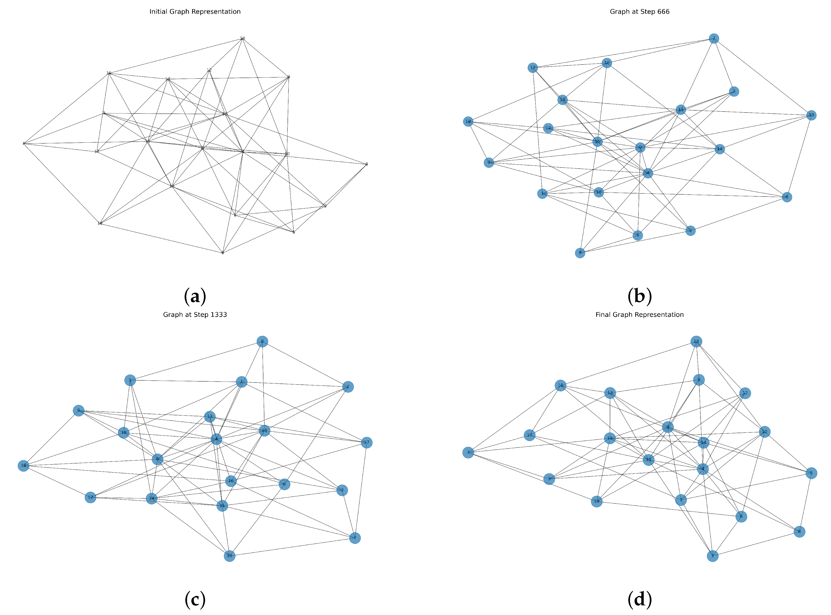
The results obtained from the simulation provide valuable insights into the evolution of both the tumoral cell population and the network’s structural properties over time. Figure 1 represents the evolution of the network, where the nodes and their connections dynamically change as new vertices and edges are introduced. This series of network graphs visualizes the dynamic evolution of a growing tumor cell network over time. Each node represents an individual unit (a region of tumor cells), and the number inside each node indicates its unique identifier (node index). The size of the nodes (bubbles) reflects the total number of tumor cells at that time step, scaled between small (10) and large (1000) for clear visual interpretation. As time progresses, the growth process leads to an increase in node sizes, reflecting the increasing tumoral cell population. Additionally, new connections and nodes modify the network’s topology, making it more interconnected over time.

Figure 1a represents the initial network configuration, where nodes are relatively sparse, and connections are randomly distributed. Figure 1b,c correspond to intermediate stages of network evolution. At these stages, new nodes have been integrated into the network, and additional edges have been introduced, leading to a more interconnected structure. Figure 1d showcases the fully evolved network, where both node count and edge density have increased significantly. The node sizes in each figure are scaled based on the population values at the corresponding time steps, visually demonstrating the growth trend.

One of the key observations from Figure 1 is that while the network expands structurally, its overall connectivity follows a non-uniform pattern due to the randomness in node attachment. Certain nodes accumulate more connections than others, hinting at an implicit preferential attachment mechanism despite the random selection process. This results in a heterogeneous degree distribution, which is often observed in real-world networks.

Moreover, the influence of stochasticity in the population model is evident when examining the node size variations over time. Fluctuations in population size directly affect the graphical representation, emphasizing how uncertainties in biological growth can propagate into structural changes in the associated network. The presence of noise ensures that the system does not follow a strictly deterministic trajectory, making the results more representative of real-world complex systems.

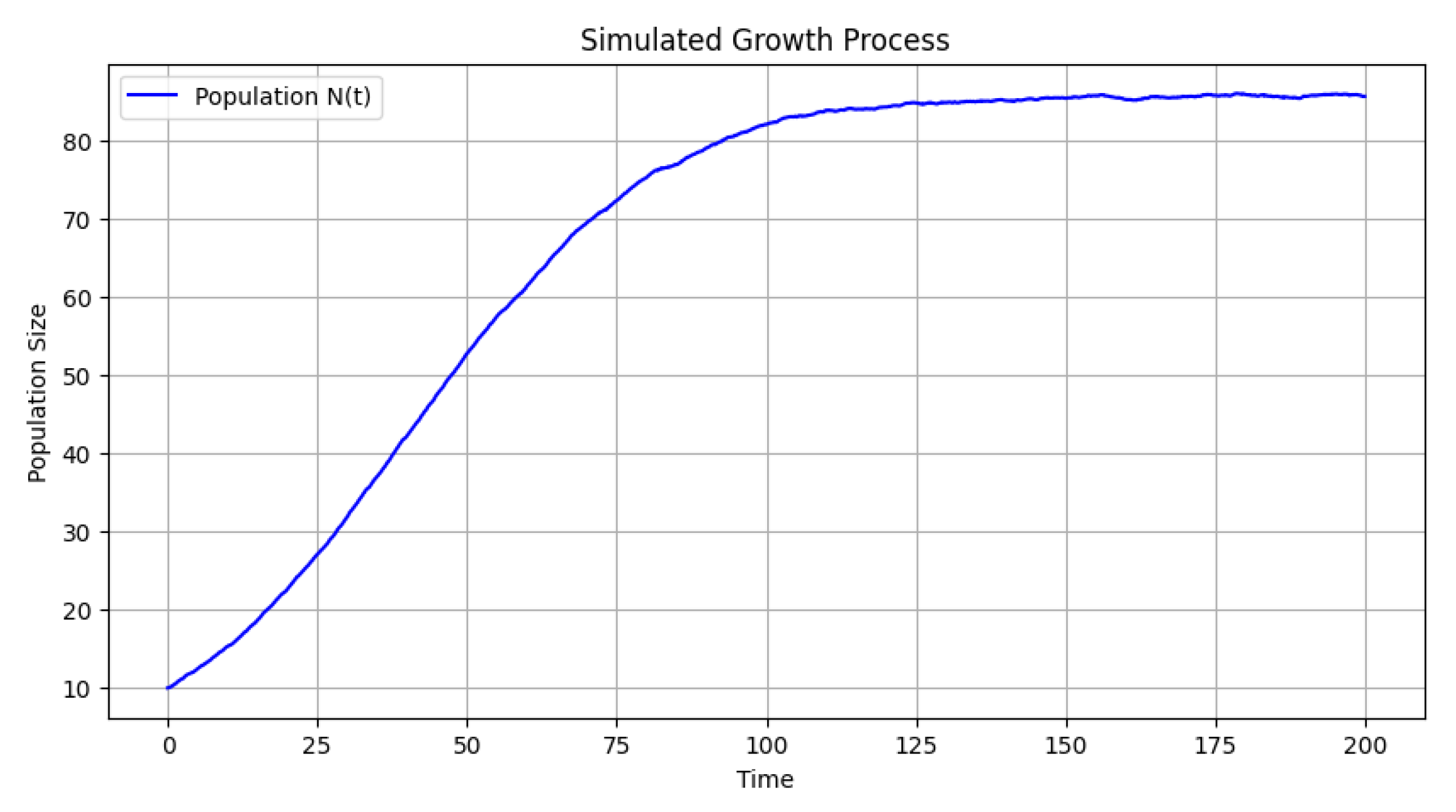
Figure 2 presents the evolution of the tumoral cell population over time. The stochastic nature of the Euler–Maruyama simulation introduces fluctuations, but overall, the population follows a growth trend influenced by carrying capacities and decay rates. The population size starts from an initial value and exhibits an increasing trajectory, with variability introduced by stochastic noise.

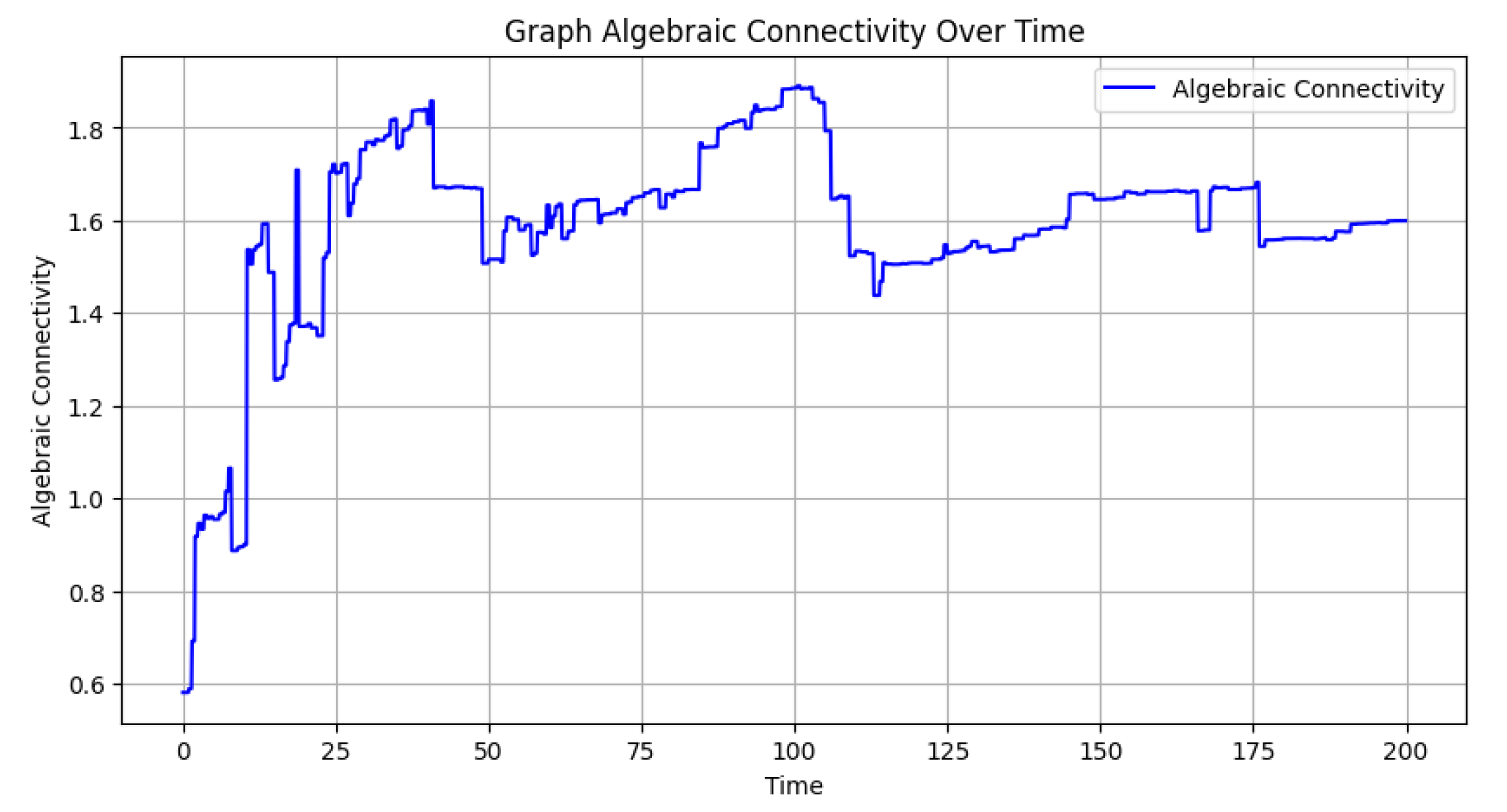
Finally, Figure 3, which presents the algebraic connectivity values for each graph, illustrates the evolution of the graph’s structural cohesion. Algebraic connectivity, derived from the Laplacian matrix’s second smallest eigenvalue, quantifies the robustness of the network. Initially, with fewer nodes and edges, the connectivity is lower, but as new nodes and connections emerge, the graph becomes more integrated, often leading to an increase in connectivity. Fluctuations in the plot indicate structural changes, such as the addition of new nodes or edges, which can temporarily disrupt or strengthen the connectivity of the network.

The simulation results provide valuable insights into the dynamic relationship between stochastic population growth and evolving network topology. The population model follows a stochastic differential equation that incorporates both logistic growth and an additional decay term. The numerical solution obtained through the Euler–Maruyama method captures both deterministic trends and random fluctuations due to the Wiener process. The results demonstrate that while the population generally follows a logistic-like growth trajectory, it is significantly influenced by stochastic perturbations, which lead to irregular oscillations around the carrying capacity. The presence of an alternative carrying capacity $K_A$ introduces an additional regulatory mechanism, creating a complex interplay between growth and decay.

The evolution of the network reflects a dynamic process where structural changes occur at predefined intervals. The initial graph is generated using an Erdös–Rényi model with a connection probability of $p=0.3$, resulting in a fairly random structure. As time progresses, new nodes are added every ten steps and connected to existing ones, while additional edges are formed between existing nodes every five steps. This leads to a gradual increase in network density and connectivity. The figures illustrate how the network expands over time, displaying an emergent structure that increasingly resembles real-world evolving systems, such as social networks or ecological food webs.

The stochastic population dynamics model and the graph evolution model operate on fundamentally different timescales, both in terms of their simulation parameters and their potential interpretations in real-world systems. These differences reflect the distinct nature of the processes they represent: one simulates rapid population changes under stochastic influences, while the other captures the slower, more structured evolution of a network over time.

The stochastic population dynamics model simulates the growth of a population influenced by both deterministic and random processes. It uses a logistic growth equation with a carrying capacity, modulated by a stochastic term that introduces environmental or demographic noise. In the simulation, this model is governed by a small time step ($\Delta t=0.1$) and a total simulation time ($T=200$), resulting in a fine-grained, continuous-like evolution of the population. At each step, a new population size is computed using the Euler–Maruyama method. Because population updates occur at every time step, this model exhibits high-frequency dynamics, allowing it to capture rapid changes over short periods.

In real-world terms, if each time step represents a day, then the entire simulation spans approximately 200 days. Depending on the species or system being modeled, this timescale can vary significantly. Thus, the model is well-suited for systems where fine temporal resolution is important, capturing detailed and fast-changing population behaviors.

In contrast, the graph evolution model simulates changes in a network structure through discrete steps. It operates by adding new nodes and edges at specific intervals: a new node with several connections is introduced every 10 steps, and additional random edges are added every 5 steps. This setup results in a slower and less frequent evolution of the graph compared to the continuous population updates. The graph changes are more structured and less reactive, emphasizing gradual development over time.

When interpreted in a real-world context, the graph represents a network of cancer cells. In this case, new nodes correspond to newly mutated or proliferated cancer cells, while the formation of new edges represents the development of cellular interactions, communication pathways, or the spread of malignancy within the tissue. These structural changes in cancerous networks typically evolve more slowly than the growth of individual cells, reflecting processes such as tumor progression, adaptation to the microenvironment, or the formation of metastatic networks over time.

Comparing the reaction timescales of the two models highlights their fundamental differences. The population model updates continuously and reacts quickly to both deterministic and stochastic influences, mimicking fast biological or ecological dynamics. In contrast, the graph model evolves more slowly and discretely, aligning with the development of cancer cell networks that unfold over extended periods. Therefore, these two models do not share a similar reaction timescale. The population model is dynamic and responsive at every simulation step, while the graph model undergoes gradual and intermittent changes, reflective of cellular systems like tumor evolution that progress at a slower pace.

11. Graph-Theoretic Insights for Targeted Therapeutic Interventions

This graph-theoretic analysis provides a powerful lens through which to interpret the complex web of interactions in the tumor microenvironment. By abstracting cells as nodes and their biochemical or physical interactions as edges, we can identify key structural and dynamical properties of the network that are predictive of disease progression or therapeutic resistance. Such properties can, in turn, inform the design of precision therapies by highlighting actionable biomarkers and vulnerable nodes or interactions.

11.1. Identification of Critical Nodes and Hubs

Centrality measures such as degree, betweenness, eigenvector, and closeness centrality can be computed to identify hub cells that serve as communication bottlenecks or major influencers in the TME as in [38]. High-degree nodes may represent tumor cells interacting with numerous immune or stromal components, indicating roles in immune modulation or microenvironment remodeling. High-betweenness nodes often bridge subpopulations, such as cancer stem cells and vasculature, making them critical targets to disrupt metastasis or angiogenesis. Eigenvector centrality identifies key coordination hubs by highlighting nodes that are well-connected to other influential nodes, potentially central to signaling or resistance mechanisms.

Such nodes can be prioritized as therapeutic targets, and their molecular profiles may serve as candidate biomarkers.

11.2. Edge Dynamics and Therapeutic Targeting of Interactions

Edges in the interaction graph encode dynamic relationships such as cytokine signaling, ligand–receptor interactions, or direct cell contact. Analyzing edge weights and temporal evolution can reveal the following:

• Stable, persistent interactions that maintain immunosuppressive microenvironments;
• Transient, high-impact signaling during invasion or metastasis initiation;
• Feedback loops or circuits involving tumor and stromal cells.

Targeting these edges corresponds to disrupting communication channels, e.g., inhibiting the PD-1/PD-L1 interaction between tumor and T cells, or blocking VEGF signaling from tumor cells to endothelial cells.

11.3. Biomarker Discovery via Node Attribute Analysis

Each node in the graph is associated with a feature vector representing molecular, phenotypic, and spatial attributes (e.g., gene expression, metabolic state, drug resistance). By correlating node centrality or influence with biological state variables, one can identify biomarkers indicative of the following:

• High metastatic potential (e.g., upregulation of MMPs or EMT markers in central nodes);
• Immunosuppressive activity (e.g., high PD-L1 expression in network hubs);
• Therapy resistance (e.g., drug-efflux transporters in peripheral, poorly connected nodes).

Machine learning techniques such as feature selection or graph neural networks can be applied to learn predictive patterns and prioritize actionable biomarkers.

11.4. Predictive Modeling and Simulation-Guided Therapy

Integrating graph–dynamics with mechanistic models allows the simulation of therapeutic perturbations (e.g., node removal, edge weakening). This enables the following:

• In silico screening of combination therapies by simulating multi-target knockdowns;
• Identification of minimal intervention sets that dismantle pro-tumor subgraphs;
• Prediction of adaptive network reconfiguration, such as emergence of compensatory pathways post-treatment.

Thus, graph-theoretic frameworks offer a mechanistic, scalable, and interpretable basis for prioritizing interventions and improving treatment specificity.

12. Conclusions and Future Work

In this study, we explored the interplay between stochastic population dynamics and the evolution of a growing network within the context of the tumor microenvironment. The population dynamics were modeled using a stochastic differential equation that incorporated tumor cell growth with logistic constraints, along with a secondary decay term and random fluctuations. The Euler–Maruyama method was employed to numerically approximate the solution, ensuring that the population (representing tumor cells) remained non-negative throughout the simulation. The results demonstrated that tumor cell populations fluctuate over time, influenced by the combined effects of deterministic growth, constraints imposed by the TME (such as nutrient limitations and immune responses), and stochastic noise.

Simultaneously, the network representing the tumor microenvironment evolved according to specific growth rules, where new cells or components (e.g., blood vessels, immune cells) were periodically introduced and connected to existing ones, while additional random interactions (e.g., tumor–stroma interactions or immune evasion mechanisms) were introduced at regular intervals. This process resulted in a dynamically expanding and changing network that exhibited characteristics of random growth models, such as preferential attachment-like behavior, despite the inherent randomness in cellular interactions. Visualizing the network at different stages revealed how its topology shifted over time, reflecting the impact of the evolving tumor population and the dynamic nature of the TME.

A key insight from this study is the connection between tumor population changes and structural adaptations in the tumor microenvironment. The mapping of tumor cell population size to node size in the network visualization highlighted how the biological process of tumor growth influenced the representation of the evolving TME. This could have significant implications for cancer research, particularly in understanding tumor evolution, metastasis, and treatment resistance, where the spatial and structural dynamics of the TME are crucial factors.

Future work could extend this model by incorporating more complex interaction rules, such as weighted edges based on the attributes of tumor and stromal cells, adaptive rewiring strategies (e.g., angiogenesis or immune evasion mechanisms), or feedback mechanisms between the network structure and tumor population dynamics. Additionally, exploring different types of noise, such as multiplicative stochasticity representing genetic mutations or environmental changes, could provide deeper insights into the stability and variability of the tumor microenvironment. Although the present study is grounded in numerical simulations, the importance of empirical validation for establishing biological relevance is fully acknowledged. Future research efforts will be directed toward validating the model’s predictions through comparison with time-lapse microscopy data of tumor organoids, as well as with growth kinetics derived from patient-specific clinical datasets. These extensions could further enhance our understanding of cancer as a complex adaptive system, where stochastic processes and network evolution are inherently linked, offering new avenues for therapeutic interventions targeting tumor–host interactions.

References

- Hanahan, D.; Weinberg, R.A. Hallmarks of Cancer: The Next Generation. Cell 2011, 144, 646–674. [Google Scholar] [CrossRef] [PubMed]
- Lodish, H.F.; Berk, A.; Kaiser, C.; Krieger, M.; Bretscher, A.; Ploegh, H.L.; Amon, A.; Martin, K.C. Molecular Cell Biology; W.H. Freeman-Macmillan Learning: New York, NY, USA, 2016. [Google Scholar]
- Verhulst, P.F. Notice sur la loi que la population suit dans son accroissement. Corresp. Mathématiqu. Phys. 1838, 10, 113–121. [Google Scholar]
- Gardiner, C.W. Stochastic Methods: A Handbook for the Natural and Social Sciences; Springer: Berlin/Heidelberg, Germany, 2009. [Google Scholar]
- Tuckwell, H.C. Introduction to Theoretical Neurobiology: Volume 2, Nonlinear and Stochastic Theories; Cambridge University Press: Cambridge, UK, 2010. [Google Scholar]
- Allen, L.J.S. An Introduction to Stochastic Processes with Applications to Biology; CRC Press: Boca Raton, FL, USA, 2010. [Google Scholar]
- Lande, R.; Engen, S.; Sæther, B.E. Stochastic Population Dynamics in Ecology and Conservation; Oxford University Press: Oxford, UK, 2003. [Google Scholar]
- Kloeden, P.E.; Platen, E. Numerical Solution of Stochastic Differential Equations; Springer: Berlin/Heidelberg, Germany, 1992. [Google Scholar]
- Quail, D.F.; Joyce, J.A. Microenvironmental regulation of tumor progression and metastasis. Nat. Med. 2013, 19, 1423–1437. [Google Scholar] [CrossRef] [PubMed]
- Newman, M.E.J. Networks: An Introduction; Oxford University Press: Oxford, UK, 2010. [Google Scholar]
- Cho, S.; Park, S.G.; Lee, D.H.; Park, B.C. Protein-protein interaction networks: From interactions to networks. J. Biochem. Mol. Biol. 2004, 37, 45–52. [Google Scholar] [CrossRef]
- Crook, O.M.; Geladaki, A.; Nightingale, D.J.H.; Vennard, O.L.; Lilley, K.S.; Gatto, L.; Kirk, P.D.W. A semi-supervised Bayesian approach for simultaneous protein sub-cellular localisation assignment and novelty detection. PLoS Comput. Biol. 2020, 16, e1008288. [Google Scholar] [CrossRef]
- Binnewies, M.; Roberts, E.W.; Kersten, K.; Chan, V.; Fearon, D.F.; Merad, M.; Coussens, L.M.; Gabrilovich, D.I.; Ostrand-Rosenberg, S.; Hedrick, C.C.; et al. Understanding the tumor immune microenvironment (TIME) for effective therapy. Nat. Immunol. 2018, 19, 541–550. [Google Scholar] [CrossRef]
- Hsieh, W.C.; Budiarto, B.R.; Wang, Y.F.; Lin, C.Y.; Gwo, M.J.; So, D.K.; Tzeng, Y.S.; Chen, S.H. Spatial multi-omics analyses of the tumor immune microenvironment. J. Biomed. Sci. 2022, 29, 96. [Google Scholar] [CrossRef]
- Helmink, B.A.; Khan, M.A.; Hermann, A.; Gopalakrishnan, V.; Wargo, J.A. The microbiome, cancer, and cancer therapy. Nat. Med. 2019, 25, 377–388. [Google Scholar] [CrossRef]
- Gogoshin, G.; Rodin, A.S. Graph Neural Networks in Cancer and Oncology Research: Emerging and Future Trends. Cancers 2023, 15, 5858. [Google Scholar] [CrossRef]
- Rodrigues, J.A. Using Physics-Informed Neural Networks (PINNs) for Tumor Cell Growth Modeling. Mathematics 2024, 12, 1195. [Google Scholar] [CrossRef]
- Tilman, D. Resource Competition and Community Structure; Princeton University Press: Princeton, NJ, USA, 1982. [Google Scholar]
- May, R.M. Simple mathematical models with very complicated dynamics. Nature 1976, 261, 459–467. [Google Scholar] [CrossRef] [PubMed]
- Murray, J.D. Mathematical Biology I: An Introduction; Springer: Berlin/Heidelberg, Germany, 2002. [Google Scholar]
- Courchamp, F.; Clutton-Brock, T.; Grenfell, B. Inverse density dependence and the Allee effect. Trends Ecol. Evol. 1999, 14, 405–410. [Google Scholar] [CrossRef]
- Hanski, I. Metapopulation Ecology; Oxford University Press: Oxford, UK, 1999. [Google Scholar]
- Yoda, K.; Kira, T.; Ogawa, H.; Hozumi, K. Self-thinning in overcrowded pure stands under cultivated and natural conditions. J. Biol. 1963, 14, 107–129. [Google Scholar]
- Lande, R. Risks of population extinction from demographic and environmental stochasticity and random catastrophes. Am. Nat. 1993, 142, 911–927. [Google Scholar] [CrossRef]
- Nisbet, R.M.; Gurney, W.S.C. Modelling Fluctuating Populations; Wiley: Hoboken, NJ, USA, 1982. [Google Scholar]
- Kutalik, Z.; Razaz, M.; Baranyi, J. Connection between stochastic and deterministic modelling of microbial growth. J. Theor. Biol. 2005, 232, 285–299. [Google Scholar] [CrossRef] [PubMed]
- Anderson, R.M.; May, R.M. Infectious Diseases of Humans: Dynamics and Control; Oxford University Press: Oxford, UK, 1991. [Google Scholar]
- Morris, W.F.; Doak, D.F. Quantitative Conservation Biology: Theory and Practice of Population Viability Analysis; Sinauer Associates: Sunderland, MA, USA, 2008. [Google Scholar]
- Holling, C.S. Resilience and stability of ecological systems. Annu. Rev. Ecol. Syst. 1973, 4, 1–23. [Google Scholar] [CrossRef]
- Scheffer, M.; Carpenter, S.; Foley, J.A.; Folke, C.; Walker, B. Catastrophic shifts in ecosystems. Nature 2001, 413, 591–596. [Google Scholar] [CrossRef]
- Albert, R.; Barabási, A.L. Statistical mechanics of complex networks. Rev. Mod. Phys. 2002, 74, 47. [Google Scholar] [CrossRef]
- Newman, M.E. The structure and function of complex networks. SIAM Rev. 2003, 45, 167–256. [Google Scholar] [CrossRef]
- Erdös, P.; Rényi, A. On random graphs. Publ. Math. 1960, 6, 290–297. [Google Scholar] [CrossRef]
- Barabási, A.L.; Albert, R. Emergence of scaling in random networks. Science 1999, 286, 509–512. [Google Scholar] [CrossRef] [PubMed]
- Jungck, J.R.; Viswanathan, R. Graph Theory for Systems Biology: Interval Graphs, Motifs, and Pattern Recognition. In Algebraic and Discrete Mathematical Methods for Modern Biology; Robeva, R.S., Ed.; Academic Press: New York, NY, USA, 2015; pp. 1–27. [Google Scholar] [CrossRef]
- Pavlopoulos, G.A.; Secrier, M.; Moschopoulos, C.N.; Soldatos, T.G.; Kossida, S.; Aerts, J.; Bagos, P.G. Using graph theory to analyze biological networks. BioData Min. 2011, 4, 10. [Google Scholar] [CrossRef] [PubMed]
- Dorogovtsev, S.N.; Mendes, J.F. Evolution of networks. Adv. Phys. 2002, 51, 1079–1187. [Google Scholar] [CrossRef]
- Rodrigues, J.A. A Topological Approach to Protein-Protein Interaction Networks: Persistent Homology and Algebraic Connectivity. Preprints 2025. [Google Scholar] [CrossRef]
Disclaimer/Publisher’s Note: The statements, opinions and data contained in all publications are solely those of the individual author(s) and contributor(s) and not of MDPI and/or the editor(s). MDPI and/or the editor(s) disclaim responsibility for any injury to people or property resulting from any ideas, methods, instructions or products referred to in the content. |
© 2025 by the author. Licensee MDPI, Basel, Switzerland. This article is an open access article distributed under the terms and conditions of the Creative Commons Attribution (CC BY) license (https://creativecommons.org/licenses/by/4.0/).