Abstract
Following various natural and man-made disasters, a critical challenge in emergency response is establishing an emergency living supplies distribution center that minimizes service costs while ensuring rapid and efficient delivery of essential goods to affected populations, thereby safeguarding their lives and material well-being. The study addresses this challenge by developing an optimization function to minimize the total service cost for locating such distribution centers, using connection points as a foundation. Utilizing a robust optimization approach that incorporates constraint conditions and bounded intervals as the value set for uncertain demand, the optimization function is transformed into a robust equivalent model through the dual principle. The tabu search method, integrated with MATLAB R2015b software, is employed to perform statistical analysis on the data, yielding the optimal solution. Case study analysis demonstrates that the minimum total service cost escalates with increases in robustness level and disturbance parameters. Furthermore, the model incorporating connection points consistently yields better results than the model without connection points, highlighting the efficacy of the proposed approach.
1. Introduction
1.1. Research Background
The 21st century has witnessed rapid advancements in human civilization, socio-economic development, and technology. However, this period has also seen a rise in issues such as population growth, ecological degradation, and resource scarcity, leading to an increasing number of both natural and man-made disasters around the world. These disasters have resulted in significant social harm that is progressively worsening. Since 2000, sudden disasters have caused global economic losses estimated at over 9 to 12 trillion US dollars [1]. For instance, the 9/11 attacks in the United States led to 2996 fatalities, while the 2010 earthquake in Chile, with a magnitude of 8.8, caused economic losses of up to 30 billion US dollars and resulted in 802 deaths. The 2015 earthquake in Nepal, with a magnitude of 8.1, caused casualties of up to 31,000 people [2]. Particularly during the COVID-19 outbreak in 2020, the cumulative global death toll exceeded 6 million by January 2022. The International Monetary Fund (IMF) projected that by 2024, the cumulative loss of global GDP could approach 13.8 trillion US dollars [3]. In China, despite its vast land area and diverse territory, resource distribution is highly uneven, presenting significant challenges for development and protection. Additionally, China’s economic development faces the triple pressures of demand contraction, supply shocks, and weakening expectations, marking a critical period. The social conflict between environmental sustainability and economic growth has become increasingly pronounced, posing a major obstacle to China’s economic progress. For example, during the SARS outbreak in 2003, the suspension of goods circulation severely impacted daily life, resulting in 349 deaths. The 2008 Wenchuan earthquake, measuring 8.0 in magnitude, caused 70,000 fatalities and economic losses of up to 840 billion yuan, both of which are the highest figures recorded in the new century. The 2008 southern snowstorm resulted in 129 deaths and required the urgent relocation of 1.66 million people, with direct economic losses exceeding 150 billion yuan. The 2010 Yushu earthquake, measuring 7.0, caused 2700 deaths and over 20 billion yuan in economic losses. Similarly, the 2013 Ya’an earthquake in Sichuan, with a magnitude of 7.0, resulted in 200 deaths, and the 2014 Ludian earthquake in Yunnan, measuring 6.5, was the largest earthquake in the province in the new century, claiming more than 600 lives. As of 13 July 2022, the COVID-19 pandemic in China has resulted in 5226 deaths and economic losses exceeding 12 trillion yuan, among other natural and non-natural disasters. These events demonstrate that such sudden disasters continually disrupt the normal development of the national economy and threaten the harmony and stability of social order.
After the outbreak of natural or man-made disasters, the government’s top priority in carrying out rescue work is to strategically determine the location of distribution centers, gather as many emergency living supplies as possible, and ensure the availability of essential goods for the affected people. However, because the demand for supplies in the disaster area far exceeds regular logistics distribution, and because basic living facilities in the disaster area are severely damaged while communication facilities are disrupted, the distribution of emergency living supplies is affected by various uncertain factors, such as user demand and transportation time. Therefore, one or more emergency supply distribution centers must be established to ensure the fastest and most efficient delivery of supplies, thereby reducing casualties and property losses. It can be seen that this location selection problem is a facility network optimization problem based on uncertain information, which involves factors such as construction costs, distribution distance, and demand volume of the distribution center. Although China’s current emergency rescue efforts prioritize relief efforts without considering costs, this approach contradicts the country’s economic principle of strict resource management and the national strategy for sustainable socio-economic development. In contrast, successful international emergency response models often consider economic factors as an essential part of decision-making [4].
After a sudden disaster, the accessibility of roads from the distribution center to aid receiving points is often inconsistent. For instance, roads may be damaged or narrowed, making it impossible for large vehicles to pass through, thus hindering the timely completion of distribution tasks. Secondly, disasters often create isolated or scattered demand points with only limited supply needs. If large vehicles are used for distribution in such cases, the efficiency and economic benefits would be significantly reduced.
To mitigate the inefficiencies caused by the aforementioned traffic conditions, establishing transfer points is essential for improving the effectiveness of emergency supply distribution.
- (1)
- Emergency supply transfer vehicles are primarily small vans, which are better suited for isolated and scattered distribution points due to their high mobility. Moreover, the operating costs of small vans are significantly lower than those of large trucks, and their higher speeds further reduce total transportation costs and time.
- (2)
- On narrow roads, small vans have better maneuverability than large trucks, allowing large vehicles to avoid difficult terrain. By utilizing transfer vehicles, the overall distribution efficiency can be significantly enhanced.
Therefore, in the process of emergency supply distribution, it is essential to strategically utilize the distinct advantages of large and small trucks, allowing them to complement each other to create a more cost-effective and efficient distribution system. This location model not only balances cost and service effectiveness but also better aligns with the real-world demands of emergency supply distribution, thereby enhancing overall efficiency. This paper draws insights from express delivery companies that use a combination of large and small trucks for feeder distribution. For example, in 2009, SF Express piloted the “mobile warehouse” strategy, which led to a significant increase in monthly collection volume and per capita efficiency after implementation [5].
1.2. Research Status and Existing Methods
The issue of distribution center location was first proposed by Hakimi S. L. based on deterministic data, predating similar research in China. In general, mathematical modeling, operations research, and other theoretical methods are commonly applied to solve this problem, leading to the gradual development of a well-established and systematic research field. The main research contributions can be categorized into three key areas: continuous location, network location, and discrete location [6]. Peidro et al. (2009) investigated the location selection of supply chain facilities, considering uncertainties in supply, demand, and distribution processes [7,8]. R. Beraldi P. and Bruni M. E. (2009) [9] proposed an optimal facility location model for emergency systems and employed a heuristic algorithm to solve the problem. Sha Y. and Huang J. (2012) [10] analyzed the decision-making challenges of post-earthquake emergency supply distribution by establishing a multi-objective location-allocation optimization model. Moreno et al. (2016) [11] developed two coordinated multi-period stochastic mixed-integer programming models to address facility location and transportation scale issues under uncertainty, thereby enhancing the efficiency of emergency response distribution. Jiahong Zhao and Ginger Y. Ke (2017) [12] examined the location selection of distribution centers under deterministic conditions using the TOPSIS method. They proposed a solution to identify the optimal model with a reasonable computation time and validated it through empirical examples. Liu Jia et al. (2017) [13] proposed an emergency material scheduling and distribution center location model based on the ant colony optimization algorithm, which accounts for fluctuating material demands and vehicle availability. Research on facility location in China began in the 1990s, lagging behind international developments. Currently, it remains in the research and development stage. Xu Chongqi, Zhang Tao, and Zeng Junwei (2015) [14] argued that the scientific selection of emergency supply distribution center locations can not only reduce costs but also enhance distribution efficiency, thereby minimizing losses caused by sudden disasters. Wang Haijun, Du Lijing et al. (2015) [15] developed a bi-objective stochastic programming model that balances cost and time under various validated its effectiveness through real-world case studies. Song Yinghua et al. (2019) [16] constructed a multi-objective location model based on dynamic demand, addressing both road damage and post-disaster recovery. Feng Jiangbo (2020) [17] developed a multi-objective optimization model within a “supply point + disaster-affected point” framework and used Wenchuan earthquake data to verify its scientific validity. Li Dongze (2020) [18] examined optimization models for distribution routes and node locations, as well as corresponding computational methods, in response to the evolving demands of the agricultural product logistics industry.
In summary, extensive research has been conducted internationally on the location selection of emergency logistics centers, employing a variety of methodologies and achieving notable results. However, domestic research on the distribution of emergency daily necessities in response to disasters remains limited (Yang Ranran, 2017) [19]. Secondly, when analyzing the location selection of emergency material distribution centers in China, most general journal articles primarily focus on location selection under deterministic conditions. Although these studies identify optimal locations, they fail to account for the impact of information uncertainty caused by sudden disasters (Song Yinghua et al., 2019) [16]. Wang Juan et al. (2017) [20] argued that if emergency material distribution prioritizes universality and timeliness while ignoring the uncertainty of material demand, it will inevitably result in a considerable waste of distribution resources. Therefore, scientifically analyzing location selection under uncertainty and optimizing the distribution of emergency supplies to meet the actual needs of each affected area will be a crucial focus for future research. In particular, when considering the role of connection points, further investigation into location selection under uncertain demand conditions is necessary [21,22,23,24].
1.3. Research Motivations
Emergency living supplies distribution, as a specialized logistics service for responding to sudden disasters, differs significantly from conventional logistics systems. Unlike modern logistics, which focuses on minimizing costs and maximizing profits, emergency logistics prioritizes rapid response and efficiency. On one hand, the development of emergency logistics began relatively late, and its distribution mechanisms lack robust data support. On the other hand, many emergencies occur unpredictably, leading to uncertainties in road traffic, delivery time, demand volume, and supply types. Furthermore, research on the optimal location selection of transfer points under parameter uncertainty, as well as the optimization of distribution routes, remains incomplete, leaving critical research gaps in this field.
Firstly, ensuring the safety of human lives and property during sudden disasters is the top priority in emergency living supplies distribution, as time is the most critical factor in disaster response. Therefore, selecting emergency supplies distribution as a research topic holds significant societal value and practical relevance in enhancing emergency response strategies.
Secondly, from a distribution process perspective, establishing transfer points and optimizing distribution center location models are crucial for advancing interdisciplinary research in emergency logistics. This research provides essential theoretical support for practical emergency distribution operations.
Thirdly, employing scientific methodologies to analyze the location selection of emergency distribution centers can offer reliable strategies and practical tools for responding to both natural and non-natural disasters. Moreover, this research contributes to strengthening the theoretical foundation of emergency logistics systems [7].
2. Constructing a Robust Optimization Location Model with Transfer Points for Minimizing Total Service Cost
2.1. Problem Description
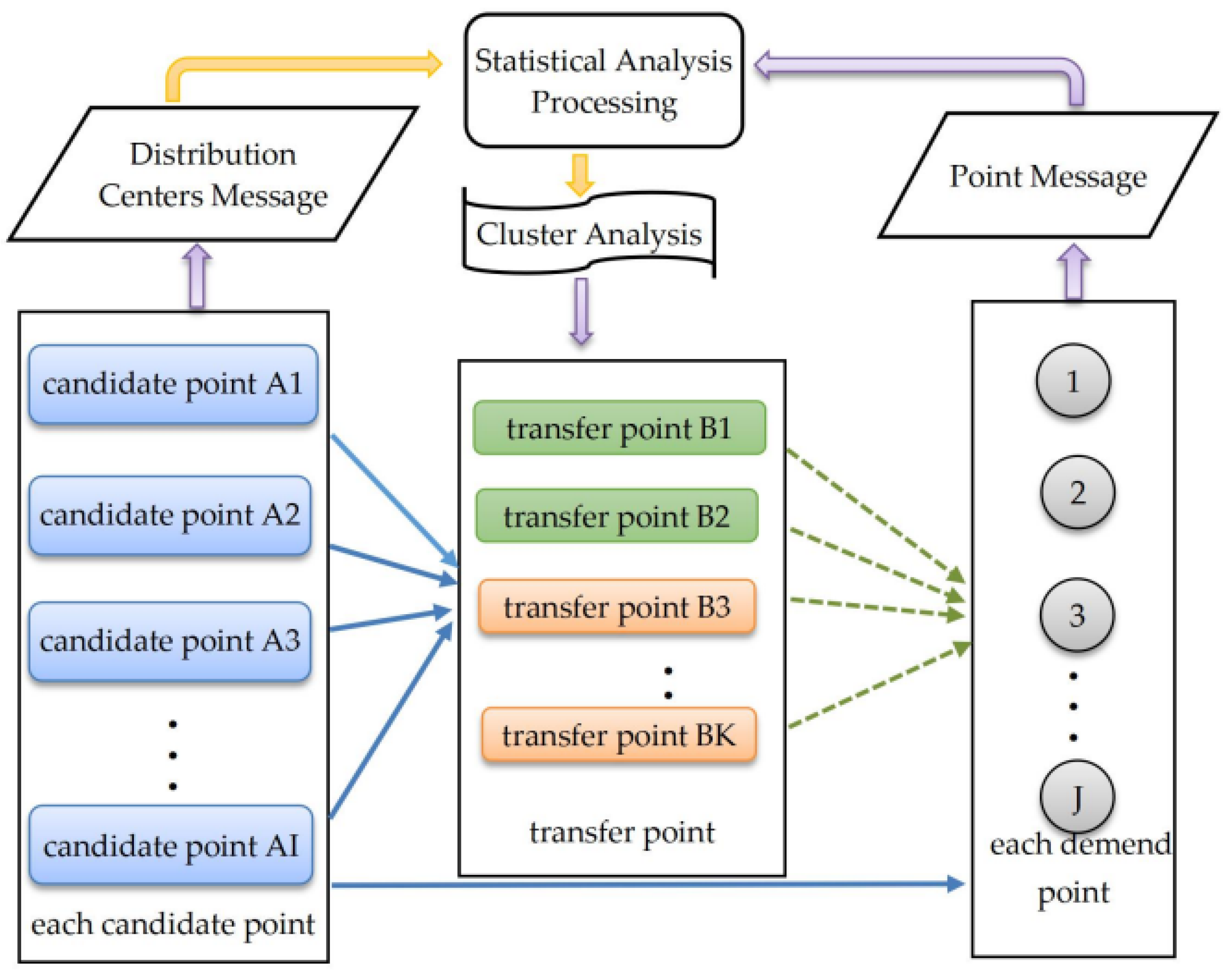
Assume there are currently I independent candidate sites for emergency life supplies distribution centers. Several distribution centers need to be established to meet the demand for emergency life supplies at J demand points, and all centers stock the same emergency supplies. Based on minimizing the total service cost, K transfer points are scientifically set up along the distribution routes. The location selection for the distribution centers is illustrated in Figure 1:
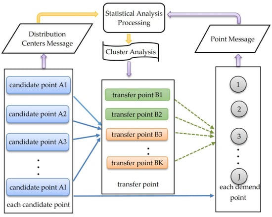
Figure 1.
Diagram of the emergency supplies distribution center location based on transshipment points.
Assume there are currently I independent candidate sites for emergency living supplies distribution centers. A certain number of distribution centers must be established to meet the demand for emergency supplies at J demand points, with all centers stocking the same types of emergency supplies.
To minimize the total service cost, K transfer points are strategically placed along the distribution routes. The location selection process for these distribution centers is illustrated in Figure 1.
The distribution vehicle A can transfer all its cargo at the transfer point(s) to one or more small transfer vehicles B, which will continue to deliver the supplies to the subsequent demand points. Specifically, the large distribution vehicle A departs from the distribution center, transports emergency life supplies to the transfer point, unloads the cargo, and then returns along the same route. The small transfer vehicle B, after loading from the large distribution vehicle at each transfer point, departs for various demand points and returns to the transfer point. The transportation costs for these supplies do not account for the empty return trips, unloading fees, time penalties, or any other expenses [25,26].
In this paper, we consider some following assumptions as:
- The construction cost for each emergency life supplies distribution center is the same and known.
- The types of vehicles used for transportation at each emergency life supplies distribution center are the same, with identical and known purchase costs for each vehicle, including those for transfer point vehicles.
- The unit storage cost for supplies at each emergency life supplies distribution center candidate point is the same and known.
- The range of distribution vehicles is sufficient to cover the total distance of each distribution route, and there are no additional costs incurred during travel.
- The unit transportation cost for supplies from each emergency life supplies distribution center to the transfer point is the same and known.
- The distances from each emergency life supplies distribution center candidate point to the transfer points and from the transfer points to the demand points are known, as are the distances between any two demand points.
- Each candidate point for the emergency life supplies distribution center can supply goods to different transfer points, with no inter-supply between distribution centers or transfer points.
- Each transfer point is supplied by multiple emergency logistics centers, and when demand arises at the transfer point, the distribution center can immediately load and deliver. Each demand point can receive supplies from multiple transfer points, and when demand arises, the transfer points can immediately load and deliver.
- Vehicle A departs from the distribution center with no intermediate assignment of delivery tasks; after unloading at a transfer point, it returns directly to the distribution center. Vehicle B departs from the transfer point with no intermediate assignment of tasks during the delivery process; after unloading at a demand point, it returns directly to the transfer point.
- All supply deliveries do not consider the time taken for vehicle loading and unloading, transfer times, or return times, and there are no time penalty costs.
- It is assumed that the total inventory capacity of all emergency life supplies distribution centers is greater than or equal to the total demand from all demand points.
2.2. Parameter Definitions
: Set of emergency life supplies demand points.
: Emergency life supplies demand point.
: Set of candidate points for emergency life supplies distribution centers.
: A candidate point for an emergency life supplies distribution center.
: Set of transfer points.
: Distance between candidate point for the i emergency life supplies distribution center and transfer point k.
: Distance between transfer point k and demand point j.
: Fixed cost of constructing an emergency life supplies distribution center at candidate point i.
: Purchase cost of each vehicle at candidate point i for the emergency life supplies distribution center.
: Purchase cost of each vehicle at transfer point k.
: Number of emergency vehicles at candidate point i, all of the same type A, with a maximum load capacity of a.
: Number of small vehicles at each transfer point k, all of the same type B, with a maximum load capacity of b.
: Unit transportation cost per unit weight per time for vehicle A from candidate point i to transfer point k.
: Unit transportation cost per unit weight per time for vehicle B from transfer point k to demand point j.
: Average speed of vehicle A, : Average speed of vehicle B.
: Travel time of vehicle A from emergency living material distribution center candidate point i to transfer point j, .
: Travel time for vehicle B from transfer point k to demand point j, .
: Unit storage cost for emergency supplies at emergency living material distribution center candidate point.
: Maximum inventory capacity at candidate point i.
: Current inventory level at candidate point i.
: Demand quantity for emergency life supplies at demand point j, with being the maximum demand at demand point j.
: Transit demand for emergency life supplies at transfer point k.
: Proportion of the demand at transfer point k that is fulfilled by distribution center i, with .
: Proportion of the demand at demand point j that is fulfilled by transfer point k, with .
is 0–1 variable, when , an emergency living material distribution center is built at candidate point i; when , not building an emergency living material distribution center at candidate point i.
H: Total budget for the construction costs of distribution centers and the purchase costs of vehicles at transfer points.
E: A sufficiently large number.
2.3. Constructing a Minimum Total Service Cost Location Optimization Model Based on Uncertain Demand
2.3.1. Location Optimization Model Based on Deterministic Demand
The total service cost function can be defined as follows [4,27,28]:
where is the construction cost of the emergency life supplies distribution center, is the storage cost of emergency life supplies at the distribution center, is the operating cost of emergency vehicle A held by the distribution center, is the operating cost of emergency vehicle B held by the transfer point, is the expected transportation cost of emergency supplies from distribution center i to transfer point k, is the expected transportation cost of emergency supplies from transfer point k to demand point j.
The sum of the above six items is referred to as the total service cost of the distribution center location. According to the economic principles of distribution centers, the objective function (1) for minimizing the total service cost can be expressed as [29,30]:
where
Constraint (3) denotes that the supply amount from each emergency life supplies distribution center cannot exceed its inventory level. Constraint (4) denotes that the supply amount from transfer points must be at least equal to the amount needed by the demand points they are responsible for supplying. Constraint (5) denotes that for each transfer point, at least one emergency life supplies distribution center is responsible for distribution, and each demand point must have at least one transfer point responsible for its supply. Constraint (6) denotes that the service volume from each emergency life supplies distribution center cannot exceed its maximum inventory capacity. Constraint (7) denotes that the maximum service volume from each transfer point must be at least equal to the maximum demand from the demand points. Constraint (8) denotes that supplies can only be delivered from locations that are selected as distribution centers. Constraint (9) denotes that only selected distribution centers can have emergency delivery vehicles. Constraint (10) denotes that the decision variables related to the number of vehicles or supply amounts are integers. Constraints (11) and (12) denotes non-negativity constraints and integrality constraints, ensuring that all supply amounts and vehicle numbers are non-negative. Constraint (13) denotes that the total costs for the construction of distribution centers and the purchase of vehicles at transfer points do not exceed the total budget H.
2.3.2. Constructing a Minimum Total Service Cost Robust Optimization Location Model Based on Uncertain Demand
In this section, we utilize robust expected optimization theory. Under the condition of having transfer points, we replace the constraints containing uncertain demand coefficients with constraints that have uncertainty sets. This transformation allows us to convert the deterministic objective function (2) into the corresponding robust model, thereby reducing the impact of uncertainty on the model.
Assume the demand is uncertain, is the nominal value of the demand and is the maximum absolute deviation, we obtain . For the demand at any given point, the uncertain demand can be divided into three parts: , , and the remainder . Given that the total demand remains unchanged, we can maximize the demand set to or , with at most one set to [31].
- (1)
- Handling uncertainty parameters and in the constraints [32,33,34,35,36,37,38].
In the aforementioned model, the demand quantity serves as a parameter in the constraints , the demand quantity serves as a parameter in the constraints , they are important parameters in (2). To unify these constraints involving uncertain demand, we will transform them as follows:
Since
we derive
Due to
Similarly, (14) can be formulated as
where
and S is the set of demand points that achieve the maximum value and , That is, S is the set of points where the demand for emergency living supplies deviates from the nominal value with demanding points attaining the maximum value. Let set {t} be the demand point with a deviation value of . Therefore, if is an integer, then the set {t} is empty; if is a non-integer, then there is one element in {t}. And , represent the set of all uncertain demand points.
When occurs, that is, no demand shift occurs, the demand at all demand points is equal to the nominal value. Therefore , constraints
represents a deterministic condition, while Model B is a demand certainty model. At this point, the model is most sensitive to uncertain quantities.
When , there are demand points in that deviate from the nominal value. Therefore, when is an integer, there are demand points in that achieve the maximum demand value, which is . Especially when occurs, meaning that all demand points have deviations in demand , the constraint condition is equivalent to the Soyster model, thus causing the demand values in the model to take their maximum values. This is obvious, and the solution of the model is overly conservative. Although the model can meet the conditions under any circumstances when the demand values change, it wastes too much cost to cope with uncertainty. When is not an integer, meaning that demand points achieve the maximum demand value, and one demand point achieves a partial deviation value. Therefore, the balance between the robustness (stability) of the model and the actual optimal solution can be controlled by adjusting the size of . Generally speaking, as increases, the robustness level of the model also increases, and the optimal solution of the objective function also increases, but its robustness becomes more stable.
Let us introduce auxiliary variables , which is satisfies , . One notes that can be transformed into the following problem
① For uncertain constraints
Due to
the dual problem of problem (15) can be expressed as:
The objective function is
Then, based on duality theory and condition (16), the uncertainty conditions can be transformed into the following equivalent constraints:
② For uncertain constraints
Due to
where can be transformed into the following dual constraints:
From Constraints (17) and (18), we obtain and have the same duality condition.
- (2)
- Handling the uncertain parameters and in the objective function.
Since the objective function
contains the uncertain demands and , the uncertainty of is caused by the uncertainty of . For convenience, let and ; then the original objective function introduces two additional constraints and . Similarly, these two additional constraints can be formulated as:
① For the constraint , we have
S is the set of demand points that achieve the maximum value, with demand points attaining the maximum value. The set {t} consists of demand points with a deviation value of . Therefore, if is an integer, then the set {t} is empty; if is a non-integer, then there is one element in {t}.
Let us introduce auxiliary variables , which is satisfies
can be transformed into the following problem:
Due to
the dual problem of problem (19) can be expressed as:
Then, based on duality theory and Condition (20), the uncertainty conditions can be transformed into the Constraints (21):
② For , due to
and
Similarly, based on duality theory, the uncertainty condition can be transformed into the equivalent Constraints (22) and (23), namely,
where .
- (3)
- Robust optimization model for total service cost.
Based on the constraints, the dual equivalent condition for the uncertainty condition is
Based on the constraints, the uncertainty condition can be transformed into the following dual constraint:
The dual equivalent expression for the constrain in the objective function is:
Similarly, the constraint in the objective function, based on duality theory, can be transformed into the equivalent constraints as follows:
where
The robust optimization model of the original objective function is:
The corresponding constraints are expressed as follow conditions:
and Conditions (5)–(13).
2.4. The Optimal Solution Model Based on Particle Swarm Optimization (PSO)
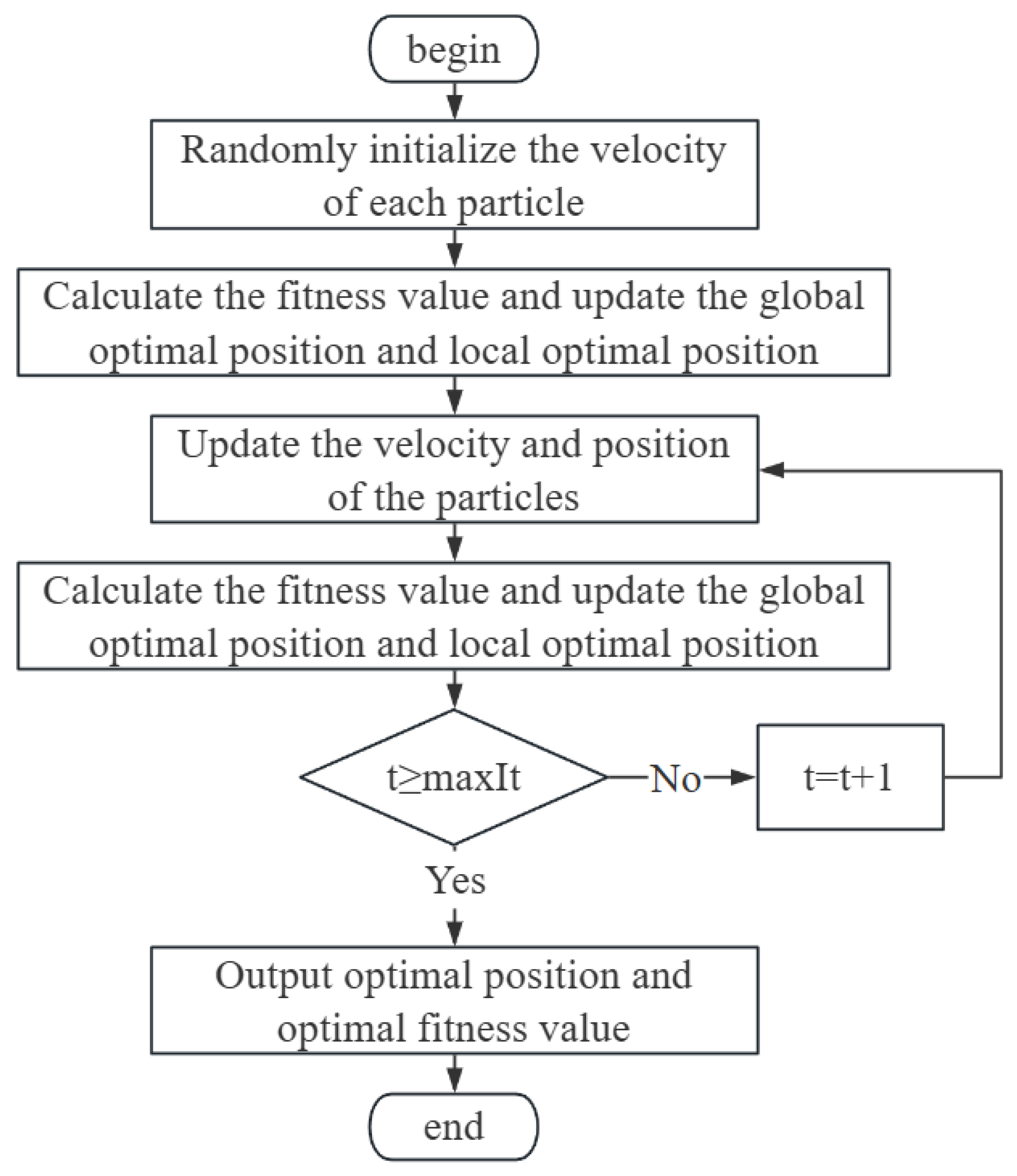
The basic idea of particle swarm algorithms revolves around “swarm” and “evolution”, in which particles are assumed to be mass- and volume-less points that fly through space at a certain speed and adjust their positions and speeds according to their individual and swarm flight experiences. The evolution equation of the particle swarm algorithm is [39,40,41,42]:
where is the particle number; is the number of spatial dimensions where the particle is located; is the number of particle iterations; is the particle velocity; is the particle position (i.e., the size of the parameter to be optimized); is the optimal position of particle in the dimension; is the optimal position of all the particles in the dimensional space; w is the inertia weight; and are the learning factors of the particle individuals and the group, and the range is 0.5~2.0; and are mutually independent random numbers with values between 0~1.
The approach of using dynamically decreasing inertia weights enables the realization of an enhanced ability to trade-off between global and local search and improves the convergence rate of the algorithm.
The dynamically decreasing expression for the inertia weights is given by
where and are the initial and final values of inertia weights, respectively; t is the current iteration number; is the total iteration number.
To better solve the above operations research problem, we consider using MATLAB to implement PSO and apply the PSO algorithm outlined above to solve problem (2), and the corresponding flowchart is presented in Figure 2.
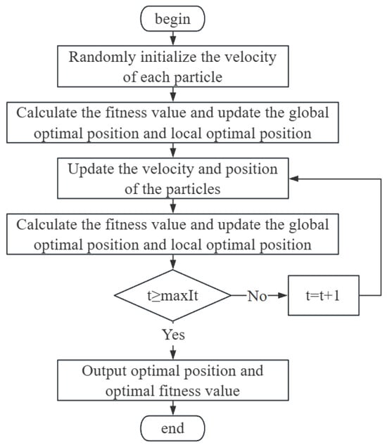
Figure 2.
The flowchart of PSO.
3. Numerical Experiments
Based on the characteristics of the model, this paper employs a heuristic algorithm based on Tabu Search (TS) to solve the location model using MATLAB software. Tabu Search is a modern heuristic algorithm that emerged in the 1980s and was proposed by Professor Fred Glover of the United States as a stochastic optimization method. It is primarily used to solve discrete combinatorial optimization problems and is a search method designed to escape local optima. Specifically, it selects an optimal solution from a finite set of solutions and does not terminate based on local optimality. Instead, it uses the maximum number of iterations as the stopping criterion, thus avoiding getting stuck in local cycles.
3.1. Model Structure Analysis
For model (24), its decision variables can be divided into two categories: one category is binary variables, such as , , ; the other category is continuous variables, such as , , , . Based on the structural characteristics of model (24), for the sake of convenience in computation, we can divide model (24) into two smaller sub-models, A and B, where model A contains only binary variables and model B contains only continuous variables.
Based on the structural characteristics of model (24), if there is for , then must exist. This indicates that only the emergency living supplies distribution center i located at the chosen site can provide emergency living supplies to demand point j. Therefore, the solution to the model is constructed as follows:
For any row, if all elements in E are 0, then the corresponding element in Y is 0; if there is a non-zero element in E, then the element in Y for that row is [4].
3.2. Model Decomposition
Divide model (24) into two parts, namely model A, which contains only binary variables, and model B, which contains only continuous variables.
① Model A is as follows:
Constraints:
② Model B is as follows:
Since model (24) is decomposed into model A and model B, the algorithmic approach for this model is as follows:
Step 1: Solve model A to obtain the values of variables and , .
Step 2: Based on the values of and , , solve model B to find the values of variables , .
Step 3: Substitute , , , , into the model to obtain the value of
thereby deriving an upper bound for the original problem.
Step 4: Repeat the above steps, continuously updating the upper bound of the objective function until the algorithm terminates.
3.3. Determine the Transfer Points
In this paper, a fast clustering analysis method is used to determine The transfer points. Therefore, based on the route characteristics of the locations of the demand points, we categorize these 10 demand points into 4 groups. Table 1 shows the distances between each demand point.

Table 1.
Distances (in kilometers) in each demand point.
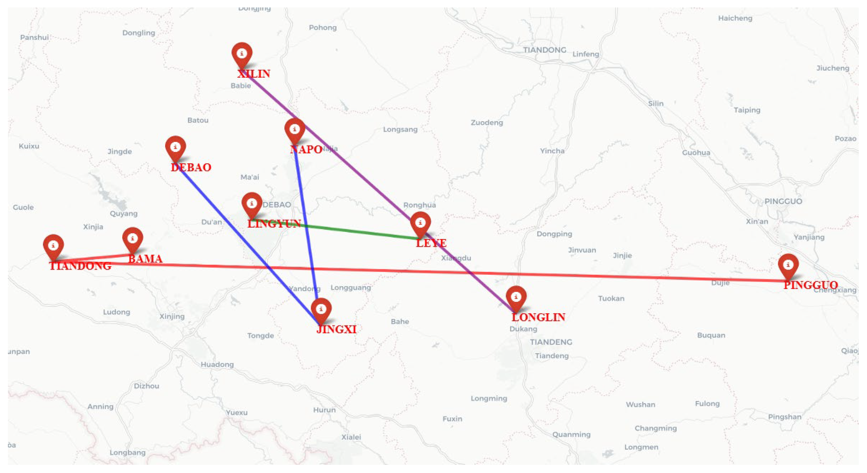
The above data were analyzed using SPSS software (IBM SPSS Statistics 26), and the results are as follows: Bama, Tiandong, and Pingguo are grouped into one category; Debao, Jingxi, and Napo into another; Leye and Lingyun into another; and Xilin and Longlin into another. The classification results reflect the positional relationships of the demand points. Since the demand points are divided into four categories, to facilitate the distribution of emergency supplies, an observation method was used to set up a transfer point for each category of demand points. The locations of the transfer points are shown in Table 2. To clearly visualize the geographical locations of these points, we used Python 3.9.7 to plot them on the Amap (Gaode) platform. As shown in Figure 3, the described locations are connected using colored lines: Bama, Tiandong, and Pingguo are linked with red lines; Debao, Jingxi, and Napo with blue lines; Leye and Lingyun with green lines; and Xilin and Longlin with purple lines.
Table 2.
Distances (in kilometers) between each site selection point and transfer points.
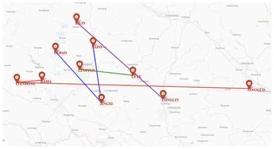
Figure 3.
Distance map of each demand point.
3.4. Case Analysis
Assume there are , , , , five candidate locations for distribution centers, representing Baise, Tianyang, Napo Town, Tianlin County, and Yongle Town. Additionally, there are ten emergency supply demand points, numbered 1 to 10, representing the demand points in Tiandong, Pingguo, Lingyun, Leye, Longlin, Bama, Xilin, Debao, Napo, and Jingxi counties. The parameter data are shown in the table below:
There are five candidate locations for distribution centers, representing Baise, Tianyang, Napo Town, Tianlin County, and Yongle Town. Additionally, ten emergency supply demand points, numbered 1 to 10, correspond to Tiandong, Pingguo, Lingyun, Leye, Longlin, Bama, Xilin, Debao, Napo, and Jingxi counties. The key parameters for site selection and demand analysis are summarized in Table 3, Table 4, Table 5 and Table 6. Table 3 presents the distances between each candidate distribution center and the emergency supply demand points. Table 4 outlines the cost parameters associated with each candidate distribution center, including construction costs, storage capacities, and transportation costs. Table 5 details the distances between transfer points and demand points, which are crucial for optimizing supply distribution. Finally, Table 6 specifies the range of demand at each demand point, providing essential data for allocation planning.
Table 3.
Distances (in kilometers) between each site selection point and demand points.
Table 4.
Cost parameters of each distribution center candidate point.
Table 5.
Distances (in kilometers) between each transfer point and demand points.
Table 6.
Range of requirements at each point of need.
We implemented the PSO (Particle Swarm Optimization) algorithm in MATLAB, setting the maximum number of iterations to 200 and the swarm size to 50. To determine the optimal values of and , we defined their range as and set the inertia weight within . The inertia weight was dynamically adjusted based on and to reach an optimal solution. As shown in Figure 4 and Table 7, the optimal values obtained were and . The number of iterations for the optimal solution is shown in Figure 5. Observing the optimization process, we found that the best solution continuously improved over iterations, demonstrating the effectiveness of the PSO algorithm in solving optimization problems.
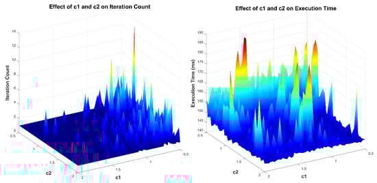
Figure 4.
Effect of and on Execution Time and Iteration Count. (Note: The closer the color is to red, the higher the Execution Time and Iteration Count, indicating longer processing time and more iterations).
Table 7.
Effect of and on Execution Time and Iteration Count.
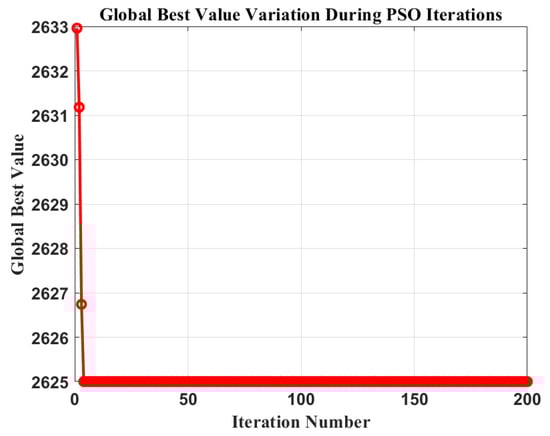
Figure 5.
Global Best Value Variation During PSO Iterations.
Therefore, under the condition of a total budget H, the reasonable planning for construction costs and vehicle purchasing costs must not exceed the total budget , which can be expressed as:
In this case study, let us assume million yuan, denoted as
The maximum loading capacity for each type vehicle is 110,000 items, denoted as . The maximum loading capacity for each type vehicle is 60,000 items, denoted as . The average speed of type vehicles is km/h, and the average speed of type vehicles is km/h. Additionally, the maximum number of iterations is set to 250.
① when , then all do not deviate, we obtain
converted to a deterministic site selection decision problem, the solution is as follows:
By this, the optimal solution of the model is
where
It is evident that among the five candidate points , only candidate points can be selected as distribution centers, while candidate points that are not selected as distribution centers. The emergency living material distribution center serves demand points 1, 2, 6, 8, 9,and 10, while the emergency living material distribution center serves demand points 3, 4, 5, 7, and 10. That is:
From Napo Town, 870,000 items are delivered to Naman, and from Naman, 250,000 items are sent to Bama, 360,000 items to Tiandong, and 260,000 items to Apple.
From Napo Town, 880,000 items are delivered to Zurong, and from Zurong, 250,000 items are sent to Debao, 360,000 items to Jingxi, and 270,000 items to Napo.
From Tianlin County, 370,000 items are delivered to Lingzhan, and from Lingzhan, 230,000 items are sent to Leye and 140,000 items to Lingyun.
From Tianlin County, 590,000 items are delivered to Wangdian, and from Wangdian, 410,000 items are sent to Longlin and 180,000 items to Xilin.
From Tianlin County, 210,000 items are delivered to Zurong, and from Zurong, 210,000 items are sent to Jingxi.
② when , the value of is related to the number of demand points deviating from the nominal value. When is an integer, it indicates that the j-th distribution center candidates has demand points with deviations from the nominal value, i.e., , where represents the maximum deviation of the demand. Under the conditions of , let us assume takes the values of 0, 5, 8, and 10, respectively, and the demand disturbance term takes the values of 0.1, 0.2, and 0.3, respectively. By adjusting the values of and , the robustness of the solution is modified. The results are shown in Table 8 below.
Table 8.
The optimal cost under uncertain demand conditions.
Table 8 shows that as increases, the robust minimum total service cost also increases. For , the larger is, the higher the degree of deviation, and the higher the total service cost. At the same time, it is found that when in is relatively large, the strategy for selecting distribution centers also changes.
For example, when , there is:
In this case, among the five candidate points , only candidate points are selected as distribution centers, while candidate points are not selected as distribution centers. The distribution center serves demand points 1, 2, and 6, the material distribution center serves demand points 8, 9, and 10, and the distribution center serves demand points 3, 4, 5, and 7. That is:
From Tianyang District, 994,000 items are delivered to Naman, and from Naman, 292,000 items are sent to Bama, 386,000 items to Tiandong, and 316,000 items to Apple.
From Napo Town, 1,154,000 items are delivered to Zurong, and from Zurong, 256,000 items are sent to Debao, 592,000 items to Jingxi, and 306,000 items to Napo.
From Tianlin County, 458,000 items are delivered to Lingzhan, and from Lingzhan, 262,000 items are sent to Leye, and 196,000 items to Lingyun.
From Tianlin County, 590,000 items are delivered to Wangdian, and from Wangdian, 410,000 items are sent to Longlin, and 180,000 items to Xilin.
It can be seen that in the case of transfer points, the robust optimal solution of the location model based on demand uncertainty increases continuously with the increase of and . At the same time, the location decision also changes. For example, in the optimized decision with , distribution center serves demand points 1, 2, 6, 8, 9, and 10, while distribution center serves demand points 3, 4, 5, 7, and 10. In the optimized decision with , distribution center serves demand points 1, 2, and 6, distribution center serves demand points 8, 9, and 10, and distribution center serves demand points 3, 4, 5, and 7.
3.5. Qualitative Results Analysis
Among the five candidate points, only some are chosen as distribution centers, while others are not. For example, Distribution Center 1 serves demand points 1, 2, and 6, while Distribution Center 2 serves demand points 8, 9, and 10. Similarly, Distribution Center 3 serves demand points 3, 4, 5, and 7.
When considering transfer points, the optimal solution based on demand uncertainty increases as certain parameters change, leading to adjustments in the location decisions. For example, when certain parameters change, Distribution Center 1 may serve different sets of demand points, while other distribution centers also shift in the demand points they serve.
These qualitative results show how the optimization model adapts to changing conditions, helping to make better decisions for resource allocation and cost reduction.
4. Conclusions
4.1. Research Conclusion
This paper investigates the location decision problem for emergency living material distribution centers and introduces a robust optimization method based on constraint conditions. It is also found that the optimal solution of the model with transfer points is smaller than that of the model without transfer points. As shown in Table 9:
Table 9.
The optimal expenditure cost under uncertain demand conditions.
4.2. Research Prospects
This paper conducts a systematic and in-depth study on the location selection of emergency living supplies distribution centers under uncertain demand and derives several optimization results, providing valuable theoretical insights for future research in this field. However, certain limitations in this study may impact the final optimization outcomes, warranting further research and exploration.
- (1)
- While this paper explores robust optimization for distribution center location, it primarily focuses on demand uncertainty and does not fully account for uncertainties in other parameters such as cost, transportation, and inventory. Future studies should further investigate these factors to enhance theoretical rigor and practical applicability.
- (2)
- In robust optimization, different uncertainty sets significantly influence the model’s outcomes. As the uncertainty set becomes more refined, the model structure grows more complex, making the solution process more challenging. This study adopts a box-type (interval) uncertainty set, but further research is needed on alternative uncertainty representations, as they may impact optimization results differently.
- (3)
- The limited sample size and small-scale dataset used in this study introduces certain constraints and potential biases in the theoretical findings. Expanding the sample size and data scope in future research will help validate the results and improve their real-world applicability.
Author Contributions
Conceptualization: D.F.; Methodology: D.F.; Software: G.L. and D.F.; Validation: Q.Z. and Y.Q.; Formal analysis: Q.Z. and Y.Q.; Investigation: G.L. and D.F.; Resources: Q.Z. and Y.Q.; Data curation: G.L. and D.F.; Writing—original draft preparation: G.L. and D.F.; Writing—review and editing: Q.Z. and Y.Q.; Visualization: D.F. and Q.Z.; Supervision: Y.Q.; Project administration: D.F. and Y.Q.; Funding acquisition: D.F. and Y.Q. All authors have read and agreed to the published version of the manuscript.
Funding
The Science and Technology Project of Guangxi (No. Guike AD23023002), and the Guangxi Key Laboratory of Automatic Detecting Technology and Instruments (No. YQ22106).
Data Availability Statement
Data are contained within the article.
Conflicts of Interest
The authors have declared no conflicts of interest.
References
- Wang, B. Research on Single Phase Emergency Location-Routing Problem. Master’s Thesis, Jilin University, Changchun, China, 2018. [Google Scholar]
- Shen, X.B. Study on the Optimization of Location-Transportation in Post-Earthquake Distribution of Emergency Materials. Master’s Thesis, Jiangsu Normal University, Nanjing, China, 2018. [Google Scholar]
- Zheng, Q.T. Research on resilience optimization of emergency logistics networks. China Saf. Sci. J. 2022, 32, 45–52. [Google Scholar]
- Fan, Y. Research on Vehicle Routing Problem of Emergency Supplies Based on Multi-Objectives After the Earthquake. Ph.D. Thesis, Shenyang University, Shenyang, China, 2014. [Google Scholar]
- Yao, Y. Research on Optimization of Distribution Route for Cold Chain Regional Logistics of Agricultural Products. Ph.D. Thesis, Thailand Zhengda Management College, Bangkok, Thailand, 2018. [Google Scholar]
- Yan, N. A review of research on location selection of logistics distribution centers at home and abroad. Mod. Commer. Ind. 2016, 34, 77–78. [Google Scholar]
- Chang, M.; Tseng, Y.; Chen, J. A scenario planning approach for the flood emergency logistics preparation problem under uncertainty. Transp. Res. Part E Logist. Transp. Rev. 2007, 43, 528–552. [Google Scholar] [CrossRef]
- Peidro, D.; Mula, J.; Poler, R.; Verdegay, J.L. Fuzzy optimization for supply chain planning under supply, demand, and process uncertainties. Fuzzy Sets Syst. 2009, 160, 2160–2178. [Google Scholar] [CrossRef]
- Beraldi, P.; Bruni, M.E. A probabilistic model applied to emergency service vehicle location. Eur. J. Oper. Res. 2009, 196, 594–601. [Google Scholar] [CrossRef]
- Sha, Y.; Huang, J. The multi-period location-allocation problem of engineering emergency blood supply systems. Syst. Eng. Procedia 2012, 3, 539–547. [Google Scholar] [CrossRef]
- Moreno, A.; Alem, D.; Ferreira, D. Heuristic approaches for the multi-period location-transportation problem with reuse of vehicles in emergency logistics. Comput. Oper. Res. 2016, 70, 98–110. [Google Scholar]
- Zhao, J.; Ke, G.Y. Incorporating inventory risks in location-routing models for explosive waste management. Int. J. Prod. Econ. 2017, 193, 66–77. [Google Scholar] [CrossRef]
- Liu, J.; Xie, K.F. Emergency materials transportation model in disasters based on dynamic programming and ant colony optimization. Kybernetes 2017, 46, 1285–1300. [Google Scholar] [CrossRef]
- Xu, C.Q.; Zhang, T.; Zeng, J.W. Research on the model of emergency logistics distribution center location selection. Logist. Technol. 2015, 34, 127–133. [Google Scholar]
- Wang, H.J.; Du, L.J.; Hu, D.; Wang, J. Emergency material distribution location-routing problem under uncertain conditions. J. Syst. Manag. 2015, 24, 555–561. [Google Scholar]
- Song, Y.H.; Su, B.B.; Huo, F.Z.; Ning, J.J.; Fang, D.H. Research on the rapid location selection of emergency material distribution centers considering dynamic demand. J. Saf. Sci. 2019, 34, 48–57. [Google Scholar]
- Feng, J.B. Research on the Combined Optimization of Emergency Logistics Location-Distribution Considering Demand Urgency Grading. Ph.D. Thesis, Lanzhou Jiaotong University, Lanzhou, China, 2020. [Google Scholar]
- Li, D.Z. Research and Development of Agricultural Product Logistics Management Information System Based on Distribution Node Location and Route Optimization. Ph.D. Thesis, Shandong Agricultural University, Jinan, China, 2020. [Google Scholar]
- Yang, S.F. Construction of China’s emergency logistics support mechanism based on emergency rescue. Bus. Econ. Res. 2020, 34, 45–52. [Google Scholar]
- Wang, J.; Zhang, W.; Li, Q. A location model for emergency supply distribution centers under uncertain demand. Syst. Eng. Theory Pract. 2017, 37, 1201–1210. [Google Scholar]
- Cao, Q.; Chen, W.X. A review of research on the site selection of emergency facilities. Comput. Eng. 2019, 45, 172–178. [Google Scholar]
- Ozdemar, L. Emergency logistics planning in natural disasters. Ann. Oper. Res. 2004, 130, 17–30. [Google Scholar]
- Sheu, J.B. Dynamic relief-demand management for emergency logistics operations under large-scale disasters. Transp. Res. Part E Logist. Transp. Rev. 2010, 46, 1–17. [Google Scholar]
- Berkoune, D.; Renaud, J.; Rekik, M.; Ruiz, A. Transportation in disaster response operations. Socio-Econ. Plan. Sci. 2012, 46, 228–237. [Google Scholar]
- Tao, Y.; Cai, J.; Zheng, L.; Hu, Z.A. LRP study of emergency logistics considering road damage. Rail. Transp. Econ. 2021, 39, 112–121. [Google Scholar]
- Zhu, J.X.; Tan, Q.M.; Cai, J.F.; Jiang, T.T. Emergency logistics distribution strategy based on dual uncertainty. Syst. Eng. 2016, 34, 8. [Google Scholar]
- Wang, H.J.; Du, L.J.; Hu, D.; Wang, J. Location-routing problem for relief distribution in emergency logistics under uncertainties. J. Syst. Manag. 2015, 24, 561–567. [Google Scholar]
- Lai, Z.Z.; Wang, Z.; Ge, D.M.; Chen, Y.L. The site selection for multi-objective emergency logistics center modeling. Oper. Res. Manag. 2020, 29, 89–99. [Google Scholar]
- Mollah, A.K.; Sadhukhan, S.; Das, P.; Anis, M.Z. A cost optimization model and solutions for shelter allocation and relief distribution in flood scenario. Int. J. Disaster Risk Reduct. 2018, 31, 155–165. [Google Scholar] [CrossRef]
- Yang, Z.Z.; Mu, X.; Zhu, X.C. Optimization model of multi-distribution center multi-demand point distribution network under changes in traffic flow. Transp. Eng. Rep. 2015, 15, 55–61. [Google Scholar]
- Tan, X.X. Research on Electric Vehicle Charging Station Location Based on Robust Optimization. Ph.D. Thesis, Beijing Institute of Technology, Beijing, China, 2016; pp. 36–37.
- Du, B.; Zhou, H. A two-stage robust optimization model for emergency facility site selection in uncertain environments. J. Hazard. Mater. 2016, 310, 30–39. [Google Scholar]
- Sun, H. Research on optimization model of emergency logistics network. China Saf. Sci. J. 2007, 17, 12–18. [Google Scholar]
- Bertsimas, D.; Sim, M. The price of robustness. Oper. Res. 2004, 52, 35–53. [Google Scholar]
- Berglund, P.G.; Kwon, C. Robust facility location problem for hazardous waste transportation. Netw. Spatial Econ. 2014, 14, 211–233. [Google Scholar]
- Bardossy, M.G.; Aghavan, S.R. Robust optimization for the connected facility location problem. Electron. Notes Discret. Math. 2013, 44, 49–54. [Google Scholar]
- Gao, L.F.; Yu, D.M.; Zhao, S.J. Robust optimization model for emergency material reserve warehouse location under uncertain demand. China Sec. Sci. J. 2015, 25, 122–129. [Google Scholar]
- Ma, C.R.; Ma, C.X. Robust optimization of hazardous material transportation routes in uncertain environments. Chin. J. Saf. Sci. 2014, 24, 95–100. [Google Scholar]
- Kang, R.; Shi, C.; Sun, X.; Li, S.; Yang, F. Method for controlling temperature cracks in mass concrete based on response surface and particle swarm algorithm. J. Cent. South Univ. 2024, 55, 4505–4518. [Google Scholar]
- Zhang, L.B. Research Based on Particle Swarm Optimization. Ph.D. Thesis, Jilin University, Changchun, China, 2004. [Google Scholar]
- Deng, Y.S. Study on the Application of Genetic Algorithms to Distribution Network Reconfiguration. Ph.D. Thesis, Chongqing University, Chongqing, China, 2002. [Google Scholar]
- Eberhart, R.C.; Kennedy, J. Particle swarm optimization. In Proceedings of the IEEE International Conference on Neural Networks, Piscataway, NJ, USA, 27 November–1 December 1995; pp. 1942–1948. [Google Scholar]


Disclaimer/Publisher’s Note: The statements, opinions and data contained in all publications are solely those of the individual author(s) and contributor(s) and not of MDPI and/or the editor(s). MDPI and/or the editor(s) disclaim responsibility for any injury to people or property resulting from any ideas, methods, instructions or products referred to in the content. |
© 2025 by the authors. Licensee MDPI, Basel, Switzerland. This article is an open access article distributed under the terms and conditions of the Creative Commons Attribution (CC BY) license (https://creativecommons.org/licenses/by/4.0/).