Introducing the Leal Method for the Approximation of Integrals with Asymptotic Behaviour: Special Functions

Abstract

This work presents the Leal method for the approximation of integrals without known exact solutions, capable of multi-expanding simultaneously at different points. This method can be coupled with asymptotic approximations and the least squares method to extend the domain of convergence. The complete elliptic integral of the first kind, the Gamma function, and the error function are treated with this new method, resulting in highly accurate and easily computable approximations, exhibiting a wide region of convergence compared to other reported works. Finally, a comparison of computing time using Fortran between our proposals and other approximations from the literature is presented and discussed.

1. Introduction

In the analysis of phenomena in sciences and engineering, it is common to encounter various types of nonlinear differential equations and integrals without exact solutions. Therefore, a common approach to understanding the behaviour of these solutions indirectly is through the application of numerical methods. Nonetheless, such algorithms suffer from several drawbacks, including false states of equilibrium, oscillations, numerical instabilities, among others. Consequently, the numerical solution obtained may not represent the real solution [1]. Therefore, a wide field of research is focused on obtaining continuous solutions in the form of analytical approximations for the real solutions of nonlinear problems.

There are several semi-analytic methods for obtaining approximate solutions, such as the Rational Perturbation Homotopy method (RPHM) [2]. In this work, the Power Extender Series method (PSEM) [3,4] serves as the basis and will be used alongside the asymptotic analysis method [5], which examines the behaviour of functions as their arguments approach infinity. This approach includes asymptotic expansions, series, estimates, and notations that are essential for deriving approximate or asymptotic solutions to problems that cannot be solved exactly. One of the key methodologies in asymptotic theory is the Euler–Maclaurin summation formula [6], which aids in analysing complex integrals and sums. In [4], the Lambert W function was approximated using PSEM. However, for large argument values, asymptotic analysis was applied, utilizing asymptotic series to obtain accurate approximations.

Special functions in mathematical physics are solutions to differential equations that model a wide range of mathematical problems. These functions are extensively used in physics to address issues in fields such as astronomy, classical mechanics, quantum mechanics, and fluid dynamics. Special functions are distinguished by their inability to be expressed as finite combinations of elementary functions through arithmetic operations or functional compositions. These functions often exhibit asymptotic behaviour, which can be analysed to understand their properties in specific limits [3]. Typically, these functions are expressed using integrals or series.

The exploration of special functions in mathematical physics began with research across various domains, including planetary motion [7], solving algebraic equations, and Runge’s discovery of errors in polynomial interpolation [8]. Additionally, these functions have been studied in relation to oscillatory motions in both classical and quantum mechanics [9] and in the analysis of specific functions in complex variables [10]. These studies have laid a robust foundation for comprehending and utilizing special functions across numerous areas of physics and mathematics.

The significance of special functions in mathematical physics lies in their extensive applications across mathematics, engineering, and daily scenarios. For instance, the normal function plays a critical role in the processing of digital images, signals, and statistics [3]. The error function is utilized in digital communication and the study of transport phenomena [3]. Fresnel functions are vital for applications such as diffraction [11], electromagnetic wave transmission, and antenna design [12]. Elliptic functions are used in mechanics and mutual inductance [11], among other areas. Additionally, the Gamma function finds applications in fields like statistics and physics [13].

In this work, we propose a novel method for approximating integrals. This method is designed to utilize asymptotic expansions [5] and correct the non-asymptotic zones by pairing the derivatives at the expansion points with respect to the trial function and the derivatives obtained through the Taylor series. This method will be referred to for simplicity as the Leal method, resulting in highly accurate approximations, and $w\left(x\right)$ represents the asymptotic series expansion [5] of the special function with a wide domain of convergence. This paper is organized as follows. First, in Section 2, the Leal method is introduced. Section 3 presents a basic introduction to the least squares method. The case studies are presented in Section 4: the complete elliptic integral $K\left(x\right)$ [13,14,15,16,17,18] of the first kind, the Gamma function $\mathsf{\Gamma }\left(x\right)$ [19,20], and the error function [3,21,22,23]. Next, a discussion on computing convergence is presented in Section 5. Then, a numerical analysis and discussion are presented in Section 6. Finally, in Section 7, the concluding remarks from this work are presented.

2. Introduction to Leal Method

In general terms, integrals can be approximated by their Taylor series [24,25] using a particular expansion point. Therefore, we can obtain the derivatives of the exact solution at a given expansion point even if we do not know its analytical formulation. Hence, the derivatives of the exact solution are expressed as follows:

$$U\left(x_k\right),U^{\prime }\left(x_k\right),U^{″}\left(x_k\right),U^{‴}\left(x_k\right),U^{\left(iv\right)}\left(x_k\right),\dots$$

(1)

where U represents the exact solution, $x_k$ is an expansion point, and the prime denotes the derivative of U with respect to x.

Now, we can express the approximation of the nonlinear problem as

$$\tilde{U}\left(x\right)=f(x,a_1,a_2,\dots ,a_n)+w\left(x\right),$$

(2)

where $\tilde{U}$ is the approximation of U, $f(x,a_1,a_2,\dots ,a_n)$ is a trial function (TF) [26], $a_i$ ($i=[1,\dots ,n]$) are n constants to be determined by this method, and $w\left(x\right)$ represents the asymptotic series expansion [5] of the special function.

Next, we match the derivatives of (1) and (2) for different expansion points to build the following system of equations:

$$\begin{array}{c}\hfill \tilde{U}\left(x_1\right)=U\left(x_1\right),{\tilde{U}}^{\prime }\left(x_1\right)=U^{\prime }\left(x_1\right),\dots ,{\tilde{U}}^{\left(m\right)}\left(x_1\right)=U^{\left(m\right)}\left(x_1\right),\\ \hfill \tilde{U}\left(x_2\right)=U\left(x_2\right),{\tilde{U}}^{\prime }\left(x_2\right)=U^{\prime }\left(x_2\right),\dots ,{\tilde{U}}^{\left(p\right)}\left(x_2\right)=U^{\left(p\right)}\left(x_2\right),\\ \hfill ⋮\\ \hfill \tilde{U}\left(x_j\right)=U\left(x_j\right),{\tilde{U}}^{\prime }\left(x_j\right)=U^{\prime }\left(x_j\right),\dots ,{\tilde{U}}^{\left(q\right)}\left(x_j\right)=U^{\left(q\right)}\left(x_j\right),\end{array}$$

(3)

where j represents the number of expansion points.

From this point, we propose two variations of the Leal method:

1.

If $n=j+(m+p+\cdots +q)$ with j expansion points, then, to obtain $\tilde{U}\left(x\right)$, we solve (3) for the a parameters using Newton–Raphson [1], among others.

2.

If $n>j+(m+p+\cdots +q)$ with j expansion points, then we solve (3) symbolically for $j+(m+p+\cdots +q)$ variables and finally use the least squares method with the remaining variables to fit $\tilde{U}\left(x\right)$ with respect to $U\left(x\right)$. The suggested interval to perform the fitting is the zone that exhibits the poorest accuracy for the pure asymptotic solution ($w\left(x\right)$).

Figure 1 illustrates the flowchart of the Leal method for approximating special functions, detailing the necessary steps. For instance, it includes the derivation of the asymptotic series of the special function represented by $w\left(x\right)$ and the approximation $\tilde{U}\left(x\right)$. An important aspect to note is the criterion $n=j+(m+p+\dots +q)$ within the diagram. If this criterion is satisfied, the first variation of the Leal method is applied, solving for the a parameters. Otherwise, the problem is solved differently, and the remaining constants are determined using the least squares method (LSM).

It is important to remark on some key aspects of this process for both variations of the method. $w\left(x\right)$ is obtained by means of asymptotic techniques and its variations. This means that we assured the accuracy of $\tilde{U}\left(x\right)$ for the limit behaviour of $U\left(x\right)$ at $x\to \mathrm{constant}$ or $x\to \pm \infty$. Another aspect to consider is that TF can be formulated using polynomial terms, rational polynomial terms, transcendental functions, and combinations, as long as its effect over $\tilde{U}\left(x\right)$ vanishes as $w\left(x\right)$ reaches the limit region. Furthermore, it is important to note that the solution of (3) produces a symbiotic relationship between f and w in order to enlarge the domain of convergence of $\tilde{U}\left(x\right)$. What is more, optionally, $U\left(x\right)$ can be transformed into another function $U_T\left(x\right)$ in order to simplify or ease the approximation of the limit region. In this case, we apply the same procedure to obtain ${\tilde{U}}_T\left(x\right)$. Later, we apply the inverse transform to recover the approximation $\tilde{U}\left(x\right)$ of the original nonlinear problem. The multiple expansion points aid to spread the error among them, extending the convergence domain of the approximation. Finally, the application of $w\left(x\right)$ is optional if ${\tilde{U}}_T\left(x\right)$ and $\tilde{U}\left(x\right)$ are adequately proposed to model the limiting behaviour, as we will see in the case study of Gamma function.

In other words, the Leal method is an approximation method inspired by the PSEM framework to solve integral problems, with the potential to address differential problems. The proposed solution consists of two parts. The first part, $w\left(x\right)$, is an asymptotic expansion series [5] of the function, for example, the special function. This expansion exhibits asymptotic characteristics; however, $w\left(x\right)$ may lack accuracy in certain neighbourhoods, such as initial regions with non-asymptotic behaviour. To address this limitation, we introduce the TF function, referred to as the trial function. This function improves the behaviour of the approximation in these challenging regions.

The PSEM method uses series decomposition (e.g., Taylor series) for both the TF function and $w\left(x\right)$. The method then matches these decompositions in terms of their derivatives, comparing them with the exact derivatives computed for specific integral or differential problems. This procedure allows for the determination of adjustment constants $a_0,a_1,\dots ,a_n$ to achieve the best possible approximation. Some of these constants can be obtained analytically by computing derivatives. Alternatively, it is possible to use the least mean squares (LMS) method to determine them. It is important to note that this decomposition process, as employed by the PSEM method, allows the approximate functions to inherit properties of the original function, such as discontinuities and other specific behaviours. These characteristics are preserved in the series expansion of the functions.

3. Least Squares Method (LSM)

The least squares method is a mathematical and statistical technique employed to determine the optimal function that fits a given set of observed data. Its primary objective is to minimize the sum of the squared residuals, the differences between the observed values and those estimated by the model. By squaring these residuals, the method assigns greater weight to larger discrepancies, thereby enhancing the precision of the estimation [1,27].

Let ($x_0,y_0$), ($x_1,y_1$), ($x_2,y_2$), ⋯, ($x_i,y_i$) be the coordinates of a data set, such that $i=0,1,2,\cdots ,n$, and the adjustment curve is $y=f(x,a_0,a_1,a_2,\cdots ,a_j)$, where $a_j$ ($j=0,1,2,\cdots$) are adjustment constants. The least squares approximations attempt to minimize the sum of the squares from the vertical distances of $y_i$ values to the ideal model $f\left(x\right)$ and obtain the model function $S(a_0,a_1,a_2,\cdots ,a_j)$, which minimizes the square error defined by

$$S(a_0,a_1,a_2,\cdots ,a_j)=\sum _{i=1}^n{(\left(y_i\right)-f(x_i,a_0,a_1,a_2,\cdots ,a_j))}^2.$$

(4)

By construction, this represents a convex quadratic form in the parameters $a_0,a_1,\dots ,a_j$ when the model f is linear with respect to these parameters. Even in the case of nonlinear models, the problem is formulated as the minimization of S, ensuring that the search for critical points corresponds to identifying minima. Thus, (4) is designed to minimize the error with respect to the sample set. To do this, partial derivatives are defined with respect to every adjustment constant, creating a system of nonlinear equations given as

$$\begin{array}{c}\hfill {\displaystyle \frac{\partial S}{\partial a_0}}={\displaystyle \frac{\partial }{\partial a_0}}\left(\sum _{i=1}^n{(\left(y_i\right)-f(x_i,a_0,a_1,a_2,\cdots ,a_j))}^2\right)=0,\\ \hfill {\displaystyle \frac{\partial S}{\partial a_1}}={\displaystyle \frac{\partial }{\partial a_1}}\left(\sum _{i=1}^n{(\left(y_i\right)-f(x_i,a_0,a_1,a_2,\cdots ,a_j))}^2\right)=0,\\ \hfill {\displaystyle \frac{\partial S}{\partial a_2}}={\displaystyle \frac{\partial }{\partial a_2}}\left(\sum _{i=1}^n{(\left(y_i\right)-f(x_i,a_0,a_1,a_2,\cdots ,a_j))}^2\right)=0,\\ \hfill ⋮\\ \hfill {\displaystyle \frac{\partial S}{\partial a_n}}={\displaystyle \frac{\partial S}{\partial a_n}}\left(\sum _{i=1}^n{(\left(y_i\right)-f(x_i,a_0,a_1,a_2,\cdots ,a_j))}^2\right)=0.\end{array}$$

(5)

The equations in (5) are obtained by setting the partial derivatives of S with respect to each parameter $a_j$ to zero. This identifies stationary points (minima, maxima, or saddle points). However, the structure of S (a sum of squares) guarantees that these points are global minima in linear cases or local minima in nonlinear cases under standard regularity conditions. The LSM inherently seeks minima because maximizing S would contradict its purpose of reducing error [28,29]. For linear models, S is strictly convex, ensuring a unique minimum. For nonlinear models, while convexity is not guaranteed, the LSM framework still targets minima by iteratively refining parameters. Second-order conditions (e.g., positive definiteness of the Hessian matrix) confirm minima, but in practice, the LSM focuses on first-order conditions for computational efficiency, relying on the problem’s formulation to avoid maxima [28,29]. By solving the system (5) for the adjustment constants $a_j$, a model can be derived that minimizes the error with respect to the given data set. This approach facilitates the creation of a continuous function in the space, optimizing the fit with the observed samples [28]. Consequently, various models can be tested, and the most suitable one can be selected based on its ability to provide the best fit. In our work, the trial function $f(x,a_0,a_1,\dots ,a_j)$ is designed to approximate the exact solution. Maximizing the error would be counterproductive; thus, the LSM’s minimization framework aligns with the goal of achieving the best fit. This is consistent with standard optimization theory and practice [28,29].

Figure 2 illustrates this methodology, where the asterisk symbol denotes the data points. Each data point $(x_i,y_i)$, where $i=1,2,3,\dots$, contributes to determining the optimal function that best represents the data set, depicted by the blue line.

4. Leal Method Applied to Approximate Special Functions

In this section, we will present the approximations for the following special functions:

$$K\left(x\right)={\int }_0^{\pi /2}{\displaystyle \frac{d\theta }{\sqrt{1-x^2{sin}^2\theta }}},$$

(6)

$$\mathsf{\Gamma }\left(x\right)={\int }_0^{\infty }{e}^{-t}{t}^{x-1}dt,$$

(7)

and

$$erf\left(x\right)={\displaystyle \frac{2}{\sqrt{\pi }}}{\int }_0^{x}exp(-t^2)dt,$$

(8)

which are the complete elliptic integral $K\left(x\right)$ [14,15,16,17,18] of the first kind, the Gamma function $\mathsf{\Gamma }\left(x\right)$ [19,20], and the error function [21,22,23], respectively. This section begins with a demonstrative case study illustrating the application of the Leal method. It is important to remark that all the power series expansions of this work were obtained applying the built-in package ”MultiSeries” of Maple 2021.

4.1. Approximation Procedure Using Variation of LEAL Method, Variant 2

To understand the application of Leal’s method, we considered the $f\left(x\right)$ given by

$$f\left(x\right)=\int \left({\displaystyle \frac{1}{x}}+1\right)dt$$

(9)

First, we will obtain the series expansion $w\left(x\right)$ for the six first terms of $f\left(x\right)$ using Maple command “series”. The series expansion for $w\left(x\right)$ is given by

$$w\left(x\right)=-{\displaystyle \frac{137}{60}}+6x-5x^2+{\displaystyle \frac{10}{3}}{x}^3-{\displaystyle \frac{5}{4}}{x}^4+{\displaystyle \frac{1}{5}}{x}^5.$$

(10)

Second, the proposed trial function is

$$\mathrm{TF}\left(x\right)={\displaystyle \frac{a_0+a_{1}x}{1+b_{0}x}}(1-x),$$

(11)

where we will obtain $a_0$ and $a_1$ analytically and $b_0$ using the LMS method. There are $n=3$ constants to be determined. Following Leal’s method, variant 2, we propose the following coupled approximation:

$$\tilde{f}\left(x\right)=w\left(x\right)+{\displaystyle \frac{a_0+a_{1}x}{1+b_{0}x}}(1-x).$$

(12)

Applying the Leal method with expansion point $X_0=0.9$, then $j=1$, $m=1$, we have $n>j+\left(m\right)$ and

Applying Leal’s method with the expansion point $X_0=0.9$, then $j=1$, $m=1$, we have $n>j+m$ and

$$\begin{array}{cc}\hfill \underset{X\to \frac{9}{10}}{lim}\tilde{f}\left(X\right)=& \underset{X\to \frac{9}{10}}{lim}f\left(X\right),\hfill \\ \hfill \underset{X\to \frac{9}{10}}{lim}{\tilde{f}}^{\prime }\left(X\right)=& \underset{X\to \frac{9}{10}}{lim}{f}^{\prime }\left(X\right).\hfill \end{array}$$

(13)

Solving (13) for $a_0$ and $a_1$, we obtain:

$$\begin{array}{c}\hfill a_0=ln\left({\displaystyle \frac{9}{10}}\right)(9b_0+10)-{\displaystyle \frac{9a_0}{10}}+{\displaystyle \frac{948243b_1}{1000000}}+{\displaystyle \frac{316081}{300000}},\\ \hfill a_1=-\left(9000000\right(9ln\left({\displaystyle \frac{9}{10}}\right)b_0+10ln\left({\displaystyle \frac{9}{10}}\right)-{\displaystyle \frac{9b_0}{10}}+\\ \hfill {\displaystyle \frac{948243b_1}{1000000}}+{\displaystyle \frac{316081}{300000}})b_0+81b_0^2+8100000a_1\\ \hfill 81000000ln\left({\displaystyle \frac{9}{10}}\right)b_0+90000000ln\left({\displaystyle \frac{9}{10}}\right)-\\ \hfill +8534367b_0+9482530)/\left(90000(81b_0+80)\right).\end{array}$$

(14)

Now, after substituting $a_0$ and $a_1$ into (12) and applying the LMS method with the NonlinearFit command of Maple in the range $x\in [0.001,0.85]$ (using 850 samples) to obtain $b_1$, we have:

$$\begin{array}{c}\hfill \tilde{f}\left(x\right)=-{\displaystyle \frac{137}{60}}+6x-5x^2+{\displaystyle \frac{10}{3}}{x}^3-{\displaystyle \frac{5}{4}}{x}^4+{\displaystyle \frac{1}{5}}{x}^5-\\ \hfill {\displaystyle \frac{49\mathsf{\Xi }\left(x\right)(x-1)}{304\left({\displaystyle \frac{1223}{18}}x+1\right)}},\\ \hfill \mathsf{\Xi }\left(x\right)=\mathsf{\Psi }\left(x\right)\left({\displaystyle \frac{1174}{17}}ln\left(10\right)-{\displaystyle \frac{1105}{8}}ln\left(3\right)\right)+\\ \hfill {\displaystyle \frac{1138}{3}}-{\displaystyle \frac{2342x}{5}},\\ \hfill \mathsf{\Psi }\left(x\right)=\left(-{\displaystyle \frac{335}{6}}+{\displaystyle \frac{1241x}{18}}\right).\end{array}$$

(15)

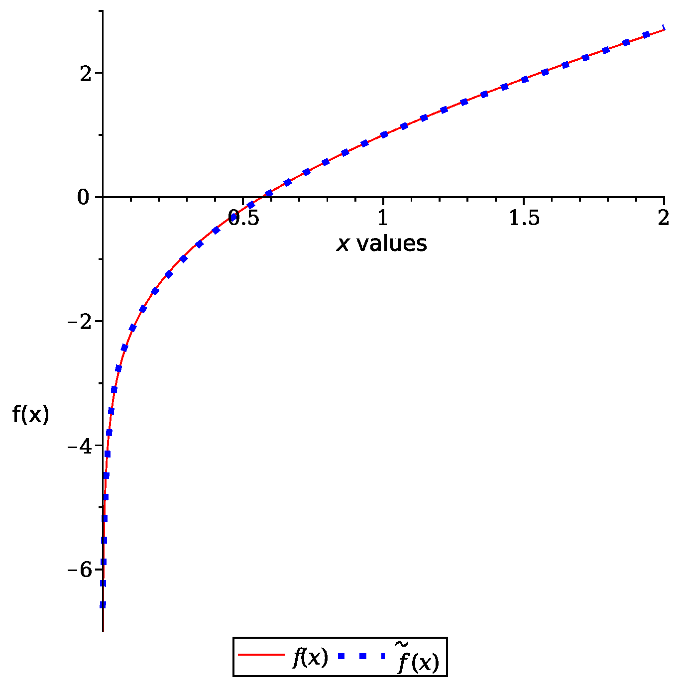
Figure 3 shows the comparison between $f\left(x\right)$ and $\tilde{f}\left(x\right)$. The figure demonstrates that they maintain good accuracy within the range $[0,2]$. The Appendix A provides the code for this case study.

4.2. Approximation Procedure for $K\left(x\right)$ Using Variation 1 of Leal Method

First, we propose the following transform

$$K_T\left(X\right)=ln\left({\displaystyle \frac{1}{K(1-X)}}+1\right),$$

(16)

where $X=1-x$.

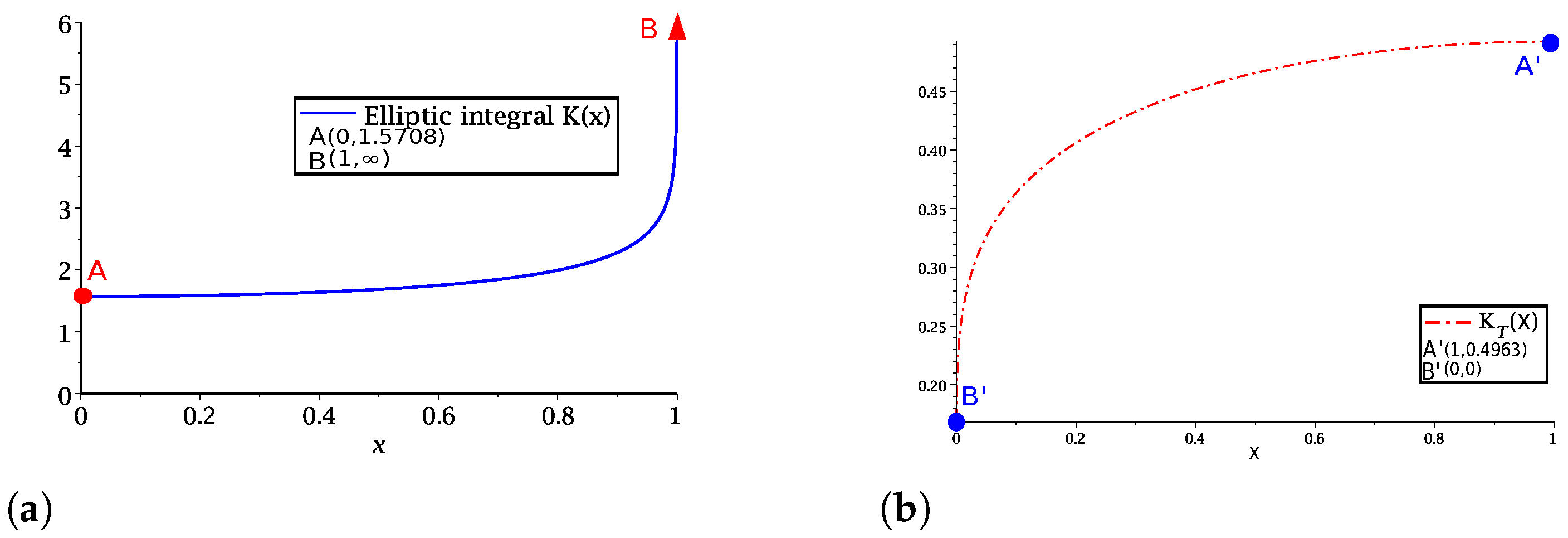
Figure 4a,b illustrate the behaviour of the complete elliptic integral $K\left(x\right)$ and its transformation $K_T\left(x\right)$ introducing the change of variable $X=1-x$ within the interval $x\in [0,1]$. It is important to notice how the A and B points and their correspondent $A^{\prime }$ and $B^{\prime }$ are swapped; in particular, the B point is projected from infinity to zero, simplifying the process of the solution.

Calculating the order two series expansion of (16) at $X=0$: results

$$\begin{array}{c}\hfill {\tilde{K}}_{T_0}\left(X\right)=ln\left({\displaystyle \frac{2+3ln\left(2\right)-ln\left(X\right)}{3ln\left(2\right)-ln\left(X\right)}}\right)-{\displaystyle \frac{(-1+3ln(2)-ln(X\left)\right)X}{(3ln(2)-ln(X\left)\right)(2+3ln(2)-ln(X\left)\right)}}.\end{array}$$

(17)

Now, we propose the trial function for this problem

$$\mathrm{TF}\left(X\right)={\displaystyle \frac{\mathsf{\xi }\left(X\right)}{\mathsf{\Phi }\left(X\right)}}={\displaystyle \frac{a_6{X}^6+a_5{X}^5+a_4{X}^4+a_3{X}^3+a_2{X}^2+a_{1}X}{b_6{X}^6+b_5{X}^5+b_4{X}^4+b_3{X}^3+b_2{X}^2+b_{1}X+1}},$$

(18)

where $\mathrm{TF}\left(X\right)$ tends to vanish in the proximity of the $X=0$ as expected, assuring the predominance of ${\tilde{K}}_{T_0}\left(X\right)$ in this region.

Then, following the Leal method, we propose the next coupled approximation

$${\tilde{K}}_T\left(X\right)=\mathrm{TF}\left(X\right)+{\tilde{K}}_{T_0}\left(X\right),$$

(19)

where $a_1,\cdots ,a_5$ and $b_1,\cdots ,b_6$ are constants to be determined by the Leal method. Now, we obtain a set of 12 equations for the derivatives at $X=1$ and $X=0.1$

$$\begin{array}{cc}\hfill \underset{X\to \frac{1}{10}}{lim}{\tilde{K}}_T\left(X\right)=& \underset{X\to \frac{1}{10}}{lim}{K}_T\left(X\right),\hfill \\ \hfill \underset{X\to \frac{1}{10}}{lim}{\tilde{K}}_T^{\prime }\left(X\right)=& \underset{X\to \frac{1}{10}}{lim}{K}_T^{\prime }\left(X\right),\cdots ,\hfill \\ \hfill \underset{X\to \frac{1}{10}}{lim}{\tilde{K}}_T^{\left(v\right)}\left(X\right)=& \underset{X\to \frac{1}{10}}{lim}{K}_T^{\left(v\right)}\left(X\right),\hfill \\ \hfill \underset{X\to 1}{lim}{\tilde{K}}_T\left(X\right)=& \underset{X\to 1}{lim}{K}_T\left(X\right),\hfill \\ \hfill \underset{X\to 1}{lim}{\tilde{K}}_T^{\prime }\left(X\right)=& \underset{X\to 1}{lim}{K}_T^{\prime }\left(X\right),\cdots ,\hfill \\ \hfill \underset{X\to 1}{lim}{\tilde{K}}_T^{\left(v\right)}\left(X\right)=& \underset{X\to 1}{lim}{K}_T^{\left(v\right)}\left(X\right),\hfill \end{array}$$

(20)

Solving (20) and substituting the result and $X=1-x$ into the inverse transform, we obtain

$$\begin{array}{cc}\hfill {\tilde{K}}_1\left(x\right)& ={\displaystyle \frac{1}{exp\left({\tilde{K}}_T(1-x)\right)-1}},0\le x\le 1,\hfill \\ \hfill {\tilde{K}}_T(1-x)& ={\displaystyle \frac{\mathsf{\xi }(1-x)}{\mathsf{\Phi }(1-x)}}+{\tilde{K}}_{T_0}(1-x),\hfill \end{array}$$

(21)

and

$$\begin{array}{c}\hfill \mathsf{\xi }(1-x)={\displaystyle \frac{77804536}{36924097}}{(1-x)}^6-{\displaystyle \frac{34920949}{11787120}}{(1-x)}^5-{\displaystyle \frac{204405104}{43666965}}{(1-x)}^4-\\ \hfill {\displaystyle \frac{7285956}{9188933}}{(1-x)}^3-{\displaystyle \frac{7482109}{385464945}}{(1-x)}^2+{\displaystyle \frac{77429}{4322012602}}(1-x),\\ \hfill \mathsf{\Phi }(1-x)=-{\displaystyle \frac{115995201}{158520115}}{(1-x)}^6+{\displaystyle \frac{10497325}{969996}}{(1-x)}^5-{\displaystyle \frac{177670556}{3625651}}{(1-x)}^4+\\ \hfill {\displaystyle \frac{66637664}{14351787}}{(1-x)}^3+{\displaystyle \frac{208027606}{1714409}}{(1-x)}^2+{\displaystyle \frac{157022980}{5140819}}-{\displaystyle \frac{151882161}{5140819}}x.\end{array}$$

(22)

4.3. Approximation of $K\left(x\right)$ Using Variation 2 of Leal Method

Let us propose the following transform:

$$K_{T1}\left(X\right)=ln\left({\displaystyle \frac{1}{K(1-X)}}+1\right).$$

(23)

Next, we obtain the order two power series of (23) at $X=0$, resulting in the following asymptotic approximation

$${\tilde{K}}_{T1}\left(X\right)=ln\left({\displaystyle \frac{2+3ln\left(2\right)-ln\left(X\right)}{3ln\left(2\right)-ln\left(X\right)}}\right),$$

(24)

Substituting (24) into the inverse of (23) and replacing $X=1-x$, we obtain

$$K_A\left(x\right)={\displaystyle \frac{3}{2}}ln\left(2\right)-{\displaystyle \frac{1}{2}}ln(1-x),$$

(25)

which is an asymptotic approximation for $K\left(x\right)$.

Now, following the Leal method procedure, we propose

$$\begin{array}{c}\hfill {\tilde{K}}_2\left(x\right)=K_A\left(x\right)+{\displaystyle \frac{p\left(x\right)}{q\left(x\right)}}(1-x^2),\\ \hfill p\left(x\right)=a_6{x}^6+a_5{x}^5+a_4{x}^4+a_3{x}^3+a_2{x}^2+a_{1}x+a_0,\\ \hfill q\left(x\right)=b_{10}{x}^{10}+b_9{x}^9+b_8{x}^8+b_7{x}^7+b_6{x}^6+b_5{x}^5+\\ \hfill b_4{x}^4+b_3{x}^3+b_2{x}^2+b_{1}x+1.\end{array}$$

(26)

Then, we construct the following system of equations

$$\begin{array}{cc}\hfill \underset{x\to 0}{lim}{\tilde{K}}_2\left(x\right)& =\underset{x\to 0}{lim}K\left(x\right),\hfill \\ \hfill \underset{x\to 0}{lim}{\tilde{K}}_2^{\prime }\left(x\right)& =\underset{x\to 0}{lim}{K}^{\prime }\left(x\right),\hfill \\ \hfill \underset{x\to 0}{lim}{\tilde{K}}_2^{″}\left(x\right)& =\underset{x\to 0}{lim}{K}^{″}\left(x\right),\hfill \end{array}$$

(27)

to satisfy $K\left(x\right)$ and its derivative at $x=0$.

Solving for $a_0$ and $a_1$, it results

$$\begin{array}{cc}\hfill a_0& ={\displaystyle \frac{1}{2}}\pi -{\displaystyle \frac{3}{2}}ln\left(2\right),\hfill \\ \hfill a_1& =-{\displaystyle \frac{1}{2}}+\left({\displaystyle \frac{1}{2}}\pi -{\displaystyle \frac{3}{2}}ln\left(2\right)\right)b_1,\hfill \\ \hfill a_2& ={\displaystyle \frac{5\pi }{8}}-{\displaystyle \frac{1}{4}}-\left(-{\displaystyle \frac{1}{2}}+\left({\displaystyle \frac{\pi }{2}}-{\displaystyle \frac{3ln\left(2\right)}{2}}\right)b_1\right)b_1+\hfill \\ \hfill & (b_2-b_1^2)\left({\displaystyle \frac{\pi }{2}}-{\displaystyle \frac{3ln\left(2\right)}{2}}\right)-{\displaystyle \frac{3ln\left(2\right)}{2}}.\hfill \end{array}$$

(28)

Now, after substituting $a_0$ and $a_1$ into (26) and applying LSM in the range of $x\in [0.001,0.85]$ (using 849 samples), we obtain

$$\begin{array}{cc}\hfill {\tilde{K}}_2\left(x\right)=& K_A\left(x\right)+{\displaystyle \frac{p\left(x\right)}{q\left(x\right)}}(1-x^2),\hfill \\ \hfill p\left(x\right)=& {\displaystyle \frac{52463}{306859}}{x}^6+{\displaystyle \frac{338323}{156484}}{x}^5-{\displaystyle \frac{1073376}{185837}}{x}^4+{\displaystyle \frac{1061399}{340464}}{x}^3+\hfill \\ \hfill & \left({\displaystyle \frac{398125}{136349}}-{\displaystyle \frac{358485ln\left(2\right)}{180098}}\right)x^2+\left(-{\displaystyle \frac{349355}{84514}}+{\displaystyle \frac{617948ln\left(2\right)}{178087}}\right)x+{\displaystyle \frac{\pi }{2}}-{\displaystyle \frac{3}{2}}ln\left(2\right),\hfill \\ \hfill q\left(x\right)=& -{\displaystyle \frac{92263}{390200}}{x}^{10}+{\displaystyle \frac{104005}{188081}}{x}^9-{\displaystyle \frac{126709}{81341}}{x}^8+{\displaystyle \frac{396130}{221997}}{x}^7+{\displaystyle \frac{679667}{105164}}{x}^6-\hfill \\ & {\displaystyle \frac{806763}{88483}}{x}^5-{\displaystyle \frac{2184029}{393237}}{x}^4+{\displaystyle \frac{835234}{87493}}{x}^3-{\displaystyle \frac{59644}{109137}}{x}^2-{\displaystyle \frac{439845}{190139}}x+1,\hfill \end{array}$$

(29)

where the values of the remaining constants were converted into equivalent fractions using the ‘convert’ command from Maple using the option ‘rational’. The term $(1-x^2)$ guarantees that the effect of TF will vanish keeping the limit behaviour of ${\tilde{K}}_2\left(x\right)$ as $x\to 1$ due to $K_A\left(x\right)$.

4.4. Approximation of $\mathsf{\Gamma }\left(x\right)$ Using Variation 1 of Leal Method

First, we propose the following transformation for the Gamma function

$$\begin{array}{c}\hfill {\mathsf{\Gamma }}_T\left(x\right)=ln\left({\displaystyle \frac{1}{10\mathsf{\Gamma }\left(x\right)}}+1\right).\end{array}$$

(30)

Figure 5a,b show the $\mathsf{\Gamma }\left(x\right)$ and ${\mathsf{\Gamma }}_{T1}\left(x\right)$ behaviour in the interval $x\in [0,2]$. It is important to notice how the A point is projected from infinity to zero ($A^{\prime }$), allowing us to obtain the derivatives of ${\mathsf{\Gamma }}_{T1}\left(x\right)$ at $x=0$.

Now, we propose the following approximation for ${\mathsf{\Gamma }}_T\left(x\right)$

$$\begin{array}{c}\hfill {\tilde{\mathsf{\Gamma }}}_T\left(x\right)={\displaystyle \frac{\mathsf{\Pi }\left(x\right)}{\mathsf{\Psi }\left(x\right)}}={\displaystyle \frac{a_5{x}^5+a_4{x}^4+a_3{x}^3+a_2{x}^2+a_{1}x+a_0}{b_6{x}^6+b_5{x}^5+b_4{x}^4+b_3{x}^3+b_2{x}^2+b_{1}x+1}},\end{array}$$

(31)

where $a_0,\cdots ,a_5$ and $b_0,\cdots ,b_5$ are constants to be determined by the Leal method. Next, we obtain a system of 11 equations for the derivatives

$$\begin{array}{cc}\hfill \underset{X\to 0}{lim}{\tilde{\mathsf{\Gamma }}}_T\left(X\right)=& \underset{X\to 0}{lim}{\mathsf{\Gamma }}_T\left(X\right),\hfill \\ \hfill \underset{X\to 0}{lim}{\tilde{\mathsf{\Gamma }}}_T^{\prime }\left(X\right)=& \underset{X\to 0}{lim}{\mathsf{\Gamma }}_T^{\prime }\left(X\right),\cdots ,\hfill \\ \hfill \underset{X\to 0}{lim}{\tilde{\mathsf{\Gamma }}}_T^{\left(vii\right)}\left(X\right)=& \underset{X\to 0}{lim}{\mathsf{\Gamma }}_T^{\left(vii\right)}\left(X\right),\hfill \\ \hfill \underset{X\to \frac{4}{3}}{lim}{\tilde{\mathsf{\Gamma }}}_T\left(X\right)=& \underset{X\to \frac{4}{3}}{lim}{\mathsf{\Gamma }}_T\left(X\right),\hfill \\ \hfill \underset{X\to \frac{4}{3}}{lim}{\tilde{\mathsf{\Gamma }}}_T^{\prime }\left(X\right)=& \underset{X\to \frac{4}{3}}{lim}{\mathsf{\Gamma }}_T^{\prime }\left(X\right),\hfill \\ \hfill \underset{X\to 2}{lim}{\tilde{\mathsf{\Gamma }}}_T\left(X\right)=& \underset{X\to 2}{lim}{\mathsf{\Gamma }}_T\left(X\right),\hfill \\ \hfill \underset{X\to 2}{lim}{\tilde{\mathsf{\Gamma }}}_T^{\prime }\left(X\right)=& \underset{X\to 2}{lim}{\mathsf{\Gamma }}_T^{\prime }\left(X\right)\hfill \end{array}$$

(32)

using three expansion points $x=[0,4/3,2]$.

Solving (32) and substituting the result into the inverse transform, we obtain

$$\begin{array}{cc}\hfill {\tilde{\mathsf{\Gamma }}}_1\left(x\right)& ={\displaystyle \frac{\frac{1}{10}}{exp\left(\frac{\Pi \left(x\right)}{\mathsf{\Psi }\left(x\right)}\right)-1}},0\le x\le 2,\hfill \\ \hfill \mathsf{\Pi }\left(x\right)& ={\displaystyle \frac{359065}{156606257}}{x}^5-{\displaystyle \frac{308164}{22170535}}{x}^4-{\displaystyle \frac{300501}{40357138}}{x}^3+{\displaystyle \frac{671569}{6173182}}{x}^2+{\displaystyle \frac{1}{10}}x,\hfill \\ \hfill \mathsf{\Psi }\left(x\right)& ={\displaystyle \frac{8641}{22448955}}{x}^6+{\displaystyle \frac{430048}{89620273}}{x}^5+{\displaystyle \frac{416525}{24162662}}{x}^4+{\displaystyle \frac{1055311}{15655050}}{x}^3+{\displaystyle \frac{2159838}{6348467}}{x}^2+{\displaystyle \frac{981206}{1750073}}x+1.\hfill \end{array}$$

(33)

It is important to notice that we circumvented the calculation of an asymptotic approximation $w\left(x\right)$ for ${\mathsf{\Gamma }}_T\left(x\right)$ because ${\tilde{\mathsf{\Gamma }}}_T\left(x\right)$ was suitable to reproduce with high accuracy the asymptotic behaviour, as x tends to the limit value at $x=0$.

4.5. Approximation of $\mathsf{\Gamma }\left(x\right)$ Using Variation 2 of Leal Method

Calculating the order two power series expansion of $\mathsf{\Gamma }\left(x\right)$ as x tends to infinity, it results in

$${\mathsf{\Gamma }}_A\left(x\right)={\displaystyle \frac{\sqrt{\frac{2\pi }{x}}+\frac{1}{12}\sqrt{\frac{2\pi }{x^3}}}{{\left(\frac{1}{x}\right)}^{x}exp\left(x\right)}}.$$

(34)

Next, by substituting (34) into (30), we obtain the following asymptotic approximation:

$${\tilde{\mathsf{\Gamma }}}_{TA}=ln\left({\displaystyle \frac{1}{10}}{\displaystyle \frac{{\left(\frac{1}{x}\right)}^{x}exp\left(x\right)}{\sqrt{\frac{2\pi }{x}}+\frac{1}{12}\sqrt{\frac{2\pi }{x^3}}}}+1\right).$$

(35)

Now, using (35) as a reference, we propose the following trial function:

$$\begin{array}{c}\hfill {\tilde{\mathsf{\Gamma }}}_{T2}=ln\left({\displaystyle \frac{1}{10}}{\displaystyle \frac{{\left(\frac{1}{x+\Delta }\right)}^{x}exp\left(x\right)+L}{\sqrt{\frac{2\pi }{x+\Delta }}+\frac{1}{12}\sqrt{\frac{2\pi }{{(x+\Delta )}^3}}}}+1\right),\\ \hfill L={\displaystyle \frac{(a_3{x}^3+a_2{x}^2+a_{1}x-1)}{(b_2{x}^2+b_{1}x+1)}}\Delta ,\\ \hfill \Delta =exp(-5x),\end{array}$$

(36)

where $\Delta$ perturbs the asymptotic behaviour of $\mathsf{\Gamma }\left(x\right)$ at $x=0$, allowing L to replicate the asymptote as x tends to zero and preserving at the same time limiting behaviour as x tends to infinity.

Next, following the Leal method, we construct the following set of equations:

$$\begin{array}{c}\hfill \underset{x\to 0}{lim}{\tilde{\mathsf{\Gamma }}}_T^{\prime }\left(x\right)=\underset{x\to 0}{lim}{\mathsf{\Gamma }}_2^{\prime }\left(x\right),\cdots ,\underset{x\to 0}{lim}{\tilde{\mathsf{\Gamma }}}_T^{\left(iii\right)}\left(x\right)=\underset{x\to 0}{lim}{\mathsf{\Gamma }}_{T2}^{\left(iii\right)}\left(x\right).\end{array}$$

(37)

Then, isolating for $a_1,a_2$ and $a_3$ from (37), it results in

$$\begin{array}{cc}\hfill a_1={\displaystyle \frac{13}{12}}\sqrt{2\pi }& -b_1-8,\hfill \\ \hfill a_2=-{\displaystyle \frac{4\sqrt{2}}{\pi }}& (\left(-{\displaystyle \frac{13}{48}}(b_1-\gamma )-{\displaystyle \frac{121}{48}}){\pi }^{3/2}+\sqrt{2}\pi \left(b_1+{\displaystyle \frac{1}{8}}{b}_2+{\displaystyle \frac{9}{2}}\right)\right),\hfill \\ \hfill a3=-{\displaystyle \frac{18\sqrt{2}}{\pi }}& \left(\right(-{\displaystyle \frac{13}{432}}{\gamma }^2+\left(-{\displaystyle \frac{13}{216}}{b}_1-{\displaystyle \frac{121}{216}}\right)\gamma -{\displaystyle \frac{121}{216}}{b}_1-{\displaystyle \frac{13}{216}}{b}_2-\hfill \\ \hfill & {\displaystyle \frac{2147}{864}}){\pi }^{3/2}+{\displaystyle \frac{13}{2592}}{\pi }^{7/2}+(b_1+{\displaystyle \frac{2}{9}}{b}_2+{\displaystyle \frac{677}{216}})\sqrt{2}\pi ).\hfill \end{array}$$

(38)

It is important to notice that $a_1$, $a_2$, and $a_3$ guarantee the derivatives at $x=0$, and they are expressed in terms of the b constants; these have to be determined by LSM. Now, substituting (36) into the inverse of (30), we obtain

$$\begin{array}{c}\hfill {\tilde{\mathsf{\Gamma }}}_2\left(x\right)={\displaystyle \frac{\sqrt{\frac{2\pi }{x+\Delta }}+\frac{1}{12}\sqrt{\frac{2\pi }{{(x+\Delta )}^3}}}{{\left(\frac{1}{x+\Delta }\right)}^{x}exp\left(x\right)+L}}.\end{array}$$

(39)

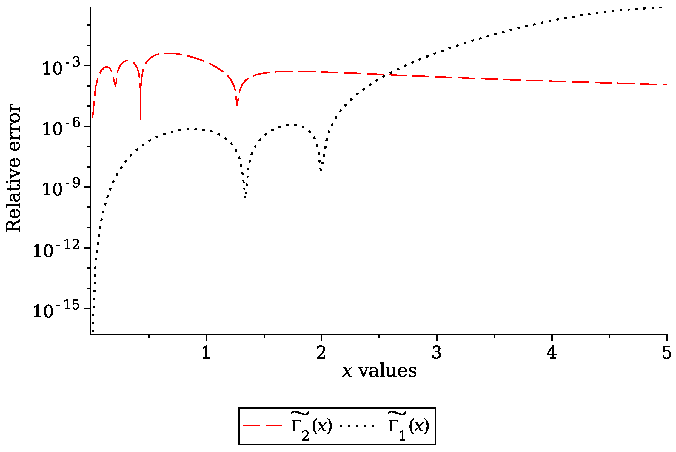
Then, we use LSM to fit ${\tilde{\mathsf{\Gamma }}}_2\left(x\right)$ in the interval of $x\in [0.01,1.2]$ (239 samples) using the remaining unknown constants, resulting $b_1=-2.09891849860793$ and $b_2=5.20339042933097$. Finally, Figure 6 displays the comparison of ${\tilde{\mathsf{\Gamma }}}_1\left(x\right)$ and ${\tilde{\mathsf{\Gamma }}}_2\left(x\right)$ with respect to $\mathsf{\Gamma }\left(x\right)$; this figure shows that they keep a good accuracy at [0,2]; however, ${\tilde{\mathsf{\Gamma }}}_1\left(x\right)$ quickly loses accuracy after $x>2.55$, while ${\tilde{\mathsf{\Gamma }}}_2\left(x\right)$ keeps it indefinitely.

Figure 7 shows that the relative error of ${\tilde{\mathsf{\Gamma }}}_1\left(x\right)$ is smaller than that of ${\tilde{\mathsf{\Gamma }}}_2\left(x\right)$ for $x<2.55$. Below this value, ${\tilde{\mathsf{\Gamma }}}_1\left(x\right)$ is more accurate than ${\tilde{\mathsf{\Gamma }}}_2\left(x\right)$. It is possible to improve the performance of ${\tilde{\mathsf{\Gamma }}}_1\left(x\right)$ and ${\tilde{\mathsf{\Gamma }}}_2\left(x\right)$ if the trial function incorporates additional adjustment constants.

4.6. Approximation of Error Function Using Variation 2 of Leal Method

First, we calculate the order two power series expansion at infinity of the error function [3,21,22,23], resulting

$$erf\left(x\right)=1-{\displaystyle \frac{1}{\sqrt{\pi }xexp\left(x^2\right)}}.$$

(40)

Next, we use (40) as a guide to propose the TF, resulting in

$$\begin{array}{c}\hfill \widetilde{erf}\left(x\right)=1-{\displaystyle \frac{1}{\sqrt{\pi }(x+\delta )exp\left(x^2\right)}},\\ \hfill \delta ={\displaystyle \frac{a_0+(a_1+(a_2+a_{3}x)x)x}{1+(b_1+(b_2+(b_3+b_{4}x)x)x)x}}.\end{array}$$

(41)

Then, in order to replicate the behaviour of $erf\left(x\right)$ at $x=0$ and its first three derivatives, we construct the following system of equations

$$\begin{array}{cc}\hfill \underset{X\to 0}{lim}\widetilde{erf}\left(X\right)=& \underset{X\to 0}{lim}erf\left(X\right),\hfill \\ \hfill \underset{X\to 0}{lim}{\widetilde{erf}}^{\prime }\left(X\right)=& \underset{X\to 0}{lim}{erf}^{\prime }\left(X\right),\cdots ,\hfill \\ \hfill \underset{X\to 0}{lim}{\widetilde{erf}}^{‴}\left(X\right)=& \underset{X\to 0}{lim}{erf}^{‴}\left(X\right).\hfill \end{array}$$

(42)

Next, we isolate $a_0,\cdots ,a_3$ from (42), resulting in

$$\begin{array}{cc}\hfill a_0& ={\displaystyle \frac{1}{\sqrt{\pi }}},\hfill \\ \hfill a_1& ={\displaystyle \frac{2}{\pi }}+{\displaystyle \frac{b_1}{\sqrt{\pi }}}-1,\hfill \\ \hfill a_2& ={\displaystyle \frac{4\sqrt{(}\pi )-{\pi }^2{b}_1+(b_2-1){\pi }^{3/2}+2b_1\pi }{{\pi }^2}},\hfill \\ \hfill a_3& =-{\displaystyle \frac{1}{{\pi }^{7/2}}}\left(\left(-2b_2+{\displaystyle \frac{8}{3}}\right){\pi }^{5/2}-8{\pi }^{3/2}+{\pi }^{7/2}{b}_2+b_1-b_3{\pi }^3-4{\pi }^2{b}_1\right).\hfill \end{array}$$

(43)

Finally, we apply LSM ($x\in [0.1,2]$ with 98 samples) to (41) in order to calculate the values of b constants, resulting in $b_1={\displaystyle \frac{3867}{3293}}$, $b_2={\displaystyle \frac{941}{1425}}$, $b_3={\displaystyle \frac{247}{1272}}$, and $b_4={\displaystyle \frac{56}{2223}}$.

5. Computing Convergence

First, we will analyse the error difference among the successive orders of variation 1 of the Leal method in order to visualize the convergence of the approximation procedure as follows:

$$\mathrm{Convergence}={\int }_a^b{({\tilde{E}}_{i+1}\left(x\right)-{\tilde{E}}_i\left(x\right))}^{2}dx,i=1,2,\dots$$

(44)

where i denotes the successive orders of the Leal $\tilde{E}$ approximations, and a and b define the chosen interval to visualize the convergence. The numerical integration was performed using the rule’s Simpson ${\displaystyle \frac{1}{3}}$.

For three case studies, we employed trial functions (TF) expressed as rational polynomial expressions of a given $[N/M]$ order, where N represents the order of the numerator and M denotes the order of the denominator.

Table 1. Calculated Convergence for the three case studies.

Case Study	Variant	Order	Chosen Interval
1	1	$i_{{\tilde{K}}_1}=[[0/0],[1/1],[2/2],\dots ,[6/6]]$	$[0,0.9999999]$
	2	$i_{{\tilde{K}}_2}[[0/0],[1/10],[2/10],\dots ,[5/10]]$	$[0,0.9999999]$
2	1	$i_{{\tilde{\mathsf{\Gamma }}}_1}=[[1/0],[1/1],\dots ,[4/4],[4/5],[5/5],[5/6]]$	$[1\times {10}^{-5},2.5]$
	2	$i_{{\tilde{\mathsf{\Gamma }}}_2}=[[0/0],[1/1],[1/2],[2/2],[3/2],[4/3],[5/4]]$	$[1\times {10}^{-7},16]$
3	2	$i_{\widetilde{erf}}=[[0/0],[0/2],[1/2],[2/2],[3/2],[3/3],[3/4]]$	$[0,3]$

shows the calculated convergence, illustrating the successive orders for the three case studies presented in this paper.

For example, for the case of the $\widetilde{\mathrm{erf}}\left(x\right)$ function, the notation $[3/4]$ indicates that the exponent of the numerator polynomial is 3 and that of the denominator is 4, continuing this pattern until reaching $[0/0]$, which signifies that the trial function vanishes. For this function, we compute the convergence by using the following successive order shown in the last row of Table 1 in the interval $[0,3]$.

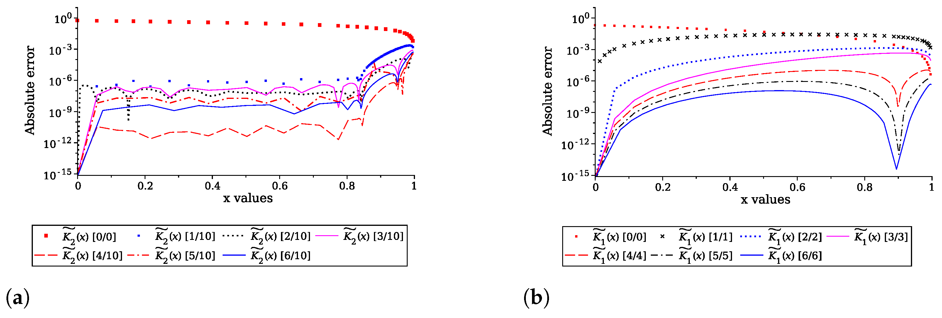
Figure 8, Figure 9 and Figure 10 show the convergence for the approximations of ${\tilde{K}}_1\left(x\right)$, ${\tilde{K}}_2\left(x\right)$, ${\tilde{\mathsf{\Gamma }}}_1\left(x\right)$, ${\tilde{\mathsf{\Gamma }}}_2\left(x\right)$, and $\widetilde{\mathrm{erf}}\left(x\right)$ for the different orders expressed in the sequences in Table 1. For the case of approximations $\tilde{\mathsf{\Gamma }}$, the error tends to reach low values below $1\times {10}^{-14}$ for ${\tilde{K}}_1$, $1\times {10}^{-10}$ for ${\tilde{K}}_2$. Additionally, it is important to highlight that the convergence behaviour of the Leal method follows the behaviour exhibited by approximate methods in the literature, such as Homotopy Analysis method (HAM) [30], Rational Homotopy Perturbation method (RHPM) [2], Variational Iteration method (VIM) [31], among others. That is, by adding more adjustment constants, convergence may present variations in accuracy, but the tendency of convergence reduces the error. This can be seen in Figure 8b and Figure 9a. The convergence of variation 2 of the Leal method relies on the least squares convergence reports from the literature [32,33,34].

Figure 11, Figure 12 and Figure 13 show the absolute error in the approximations obtained using the successive orders of the Leal $\tilde{E}$ approximations for $\mathsf{\Gamma }\left(x\right)$, $K\left(x\right)$, and $\mathrm{erf}\left(x\right)$. The absolute error decreases as N and M in $[N/M]$ increase in the trial function. It is important to note, as shown in Figure 9b, that the absolute error for ${\tilde{K}}_2\left(x\right)[4/10]$ is smaller than that for ${\tilde{K}}_2\left(x\right)[6/10]$. This behaviour arises because the convergence at iteration 5 is greater than that at iteration 6, as observed in Figure 8b. It is worth mentioning that the convergence behaviour of the Leal method aligns with the behaviour exhibited by other approximation methods reported in the literature [2,30,31], among others. In general, the absolute behaviour shown in Figure 11, Figure 12 and Figure 13 is in good agreement with the convergence behaviour presented in Figure 8, Figure 9 and Figure 10.

6. Numerical Comparison and Discussion

The Leal method employs asymptotic expansions [5] and corrects the non-asymptotic regions by matching the derivatives at the expansion points with respect to the test function and those derived from the Taylor series. This technique effectively reconstructs the initial regions exhibiting non-asymptotic behaviour, as demonstrated by the approximate functions in the case studies presented in this paper. Once the system is configured with the adjustment constants, the Leal method enables the values of $\tilde{F}\left(x\right)$ and their corresponding derivatives to be satisfied at the selected expansion points according to the chosen order. Users have the flexibility to select the expansion points and the maximum order of the derivative they wish to guarantee. Notably, this method inherently allows for the continuous entanglement of $\tilde{F}\left(x\right)$ and its derivatives relative to the exact solution. Additionally, it is important to mention that variant 2 continues to meet the requirements for the derivatives at the expansion points while simultaneously allowing for the existence of adjustment constants between $\tilde{U}\left(x\right)$ and $U\left(x\right)$.

Figure 14 presents the significant digits comparison among our proposals (${\tilde{K}}_1\left(x\right)$ and ${\tilde{K}}_2\left(x\right)$) and other reported approximations given by (A1)–(A5) from literature [13,14,15,17,18], see the equations in the Appendix A. It is important to notice that our proposals are the only ones that keep a good accuracy along the interval, exhibiting a clear advantage after $x=0.5$, in particular in the proximity to $x=1$ where $K\left(x\right)$ tends to infinity. Likewise, Figure 14 shows the result of 10 significant digits of precision for ${\tilde{K}}_1\left(x\right)$,and it is compatible with standard float (32 bit IEEE 754) of C/C++ due to its 7 digits of precision [35]. On the other hand, ${\tilde{K}}_2\left(x\right)$ exhibits a better accuracy than ${\tilde{K}}_1\left(x\right)$ particularly in the interval of $[0.2,0.8]$.

Likewise, Figure 15a shows a comparison of our approaches ${\tilde{\mathsf{\Gamma }}}_1\left(x\right)$, ${\tilde{\mathsf{\Gamma }}}_2\left(x\right)$ versus others from the literature (A6), (A7), published in [19,20], and (A8), (A9) published in [13]. It shows how ${\tilde{\mathsf{\Gamma }}}_1\left(x\right)$ reaches 7 S.D. or more in the interval of $x\in [0,2]$, while ${\tilde{\mathsf{\Gamma }}}_2\left(x\right)$ depicts more than 3 digits in the poorest zone but replicates with high accuracy both asymptotic regions ($x\to 0$ and $x\to \infty$). Note that ${\tilde{\mathsf{\Gamma }}}_1$ and ${\tilde{\mathsf{\Gamma }}}_2$ present more significant digits near $x=0$ than all other approximations in the literature.

Figure 15b demonstrates that $\widetilde{\mathrm{erf}}\left(x\right)$ provides more significant digits for $x>0.5$ compared to all the approximations (A10)–(A12) reported in [21,23] and [3], respectively. In each case, the significant digits (S.D.) [36] are calculated using...

$$\mathrm{Significant}\mathrm{Digits}\sim -{log}_{10}\left|{\displaystyle \frac{H\left(x\right)-\tilde{H}\left(x\right)}{H\left(x\right)}}\right|,$$

(45)

where $H\left(x\right)$ is the exact solution (numerical solution from Maple), and $\tilde{H}\left(x\right)$ is the approximate solution.

The Leal method is an interesting tool for the approximate solution of special functions. Moreover, future work is required to extend the power of the Leal method for the approximation of nonlinear differential equations of initial value and boundary value, fractal calculus, fractional calculus, among others. It is important to propose a systematic procedure for the selection of suitable trial functions and conduct more research on the convergence of the proposed method. Currently, we propose the trial function in order to increase the accuracy of the poorest zone while maintaining accuracy in the asymptotic region.

We can find in the literature several approximation techniques applied to integrals. Among them, we can mention the Variational Iteration method, Taylor series, Adomian Decomposition method, Successive Approximations method, Laplace Transform method, Series Solution method, and asymptotic techniques [37].

We can mention some advantages of the Leal method over the above-mentioned techniques:

♣

The Leal method is capable of providing algebraic expressions, similar to other approximation techniques.

♣

The Leal method can be coupled to work in combination with power series expansions and asymptotic expansions, as reported in the case studies of this work. This strategy can produce a remarkable increase in the domain of convergence (see case studies). In fact, further research will focus on exploring the combination of the Leal method with the Variational Iteration Method, Adomian Decomposition Method, among others.

♣

The Leal method can be applied without requiring the aforementioned coupling with other approximate methods (see Variation 1 of the Leal method in Section 4.2 and Section 4.4). In this case, the Leal method can be applied using basic knowledge of calculus and numerical methods; in contrast, some approximate methods are too cumbersome and require specialized knowledge. Taking these advantages into account, this method can also be applied to solve nonlinear ordinary differential equations.

Further research is required to explore the possibility of replacing the least squares method with a variational principle [38,39,40] to optimize some constants from the Leal method. The order of convergence and the theorem of convergence of the Leal method are open problems that deserve further work. This is a hard task that involves trial function selection and the nature of the integral to solve. Likewise, it is important to develop a systematic methodology for selecting the most appropriate trial functions prior to applying the least squares method to optimize its application. On the other hand, further research is needed to develop enhanced approximations that are compatible with the 64-bit IEEE 754 representation, ensuring 15 significant digits for all intervals of the approximations discussed in the presented case studies.

7. Conclusions

In this paper, we introduced Leal’s method for approximating special functions. The approximations were derived using various methodologies, including the Taylor series of the exact function equated with the Taylor series of the trial function (TF), asymptotic analysis, least squares, and a multiple expansion concept. Importantly, approaches using Leal’s method demonstrated superior performance in the asymptotic regions of each special function examined in the case studies. The Leal method can be combined with other approximate methods such as HPM, Padé, among others. One advantage of combining the least squares method (LSM) with Leal’s method is the extended convergence domain in regions exhibiting asymptotic behaviour. Overall, the approximations obtained with Leal’s method in the asymptotic zones showed more significant digits than other approximations found in the literature. Leal’s method has demonstrated an easy-to-apply methodology, with potential applications for solving nonlinear ordinary differential equations.

References

1. Burden, R.L.; Faires, J.D. Numerical Analysis; Cengage Learning: Singapore, 2010. [Google Scholar]
2. Saad-Albalawi, K.; Saad-Alkahtani, B.; Kumar, A.; Goswami, P. Numerical Solution of Time-Fractional Emden–Fowler-Type Equations Using the Rational Homotopy Perturbation Method. Symmetry 2023, 15, 258. [Google Scholar] [CrossRef]
3. Sandoval-Hernandez, M.A.; Vazquez-Leal, H.; Filobello-Nino, U.; Hernandez-Martinez, L. New handy and accurate approximation for the Gaussian integrals with applications to science and engineering. Open Math. 2019, 17, 1774–1793. [Google Scholar] [CrossRef]
4. Vazquez-Leal, H.; Sandoval-Hernandez, M.; Garcia-Gervacio, J.; Herrera-May, A.; Filobello-Nino, U. PSEM approximations for both branches of Lambert function with applications. Discret. Dyn. Nat. Soc. 2019, 2019, 8267951. [Google Scholar] [CrossRef]
5. de Brujin, N.G. Asymptotic Methods in Analysis; Dover: Amsterdm, The Netherlands, 1961. [Google Scholar]
6. Jakimczuk, R. Some Applications of the Euler-Maclaurin Summation Formula. Int. Math. Forum 2013, 8, 9–14. Available online: https://www.m-hikari.com/imf/imf-2013/1-4-2013/jakimczukIMF1-4-2013.pdf (accessed on 10 December 2024). [CrossRef]
7. Herschel, J.F. A Brief Notice of the Life, Researches, and Discoveries of Friedrich Wilhelm Bessel; G. Barclay: Trangie, NSW, Australia, 1847. [Google Scholar]
8. Butzer, P.; Jongmans, F. PL Chebyshev (1821–1894): A guide to his life and work. J. Approx. Theory 1999, 96, 111–138. [Google Scholar] [CrossRef]
9. Schrödinger, E. An Undulatory Theory of the Mechanics of Atoms and Molecules. Phys. Rev. 1926, 28, 1049–1070. [Google Scholar] [CrossRef]
10. Muñoz, J.L. Riemann: Una visión Nueva de la Geometría; Nivola: New York, NY, USA, 2006. [Google Scholar]
11. Sandoval-Hernandez, M.; Vazquez-Leal, H.; Hernandez-Martinez, L.; Filobello-Nino, U.; Jimenez-Fernandez, V.; Herrera-May, A.; Castaneda-Sheissa, R.; Ambrosio-Lazaro, R.; Diaz-Arango, G. Approximation of Fresnel integrals with applications to diffraction problems. Math. Probl. Eng. 2018, 2018, 4031793. [Google Scholar] [CrossRef]
12. Aznar, Á.C.; Roca, L.J.; Casals, J.M.R.; Robert, J.R.; Boris, S.B.; Bataller, M.F. Antenas; Alfaomega: London, UK, 2004. [Google Scholar]
13. Sandoval-Hernández, M.; Hernández-Méndez, S.; Torreblanca-Bouchan, S.E.; Díaz-Arango, G.U. Actualización de contenidos en el campo disciplinar de matemáticas del componente propedéutico del bachillerato tecnológico: El caso de las funciones especiales. RIDE Rev. Iberoam. Investig. Desarro. Educ. 2021, 12, 23. [Google Scholar] [CrossRef]
14. Rohedi, A.Y.; Pramono, Y.H.; Widodo, B.; Yahya, E. The Novelty of Infinite Series for the Complete Elliptic Integral of the First Kind. Preprints 2016. [Google Scholar] [CrossRef]
15. Guedes, E.; Gandhi, K.R.R. On the Complete Elliptic Integrals and Babylonian Identity II: An Approximation for the Complete Elliptic Integral of the first kind. Bull. Math. Sci. Appl. 2013, 2, 72–78. [Google Scholar] [CrossRef]
16. Borwein, J.M.; Borwein, P.B. Pi and the AGM; Wiley: New York, NY, USA, 1987. [Google Scholar]
17. Abramowitz, M.; Stegun, I.A. Handbook of Mathematical Functions with Formulas, Graphs, and Mathematical Tables; National Bureau of Standards: Gaithersburg, MD, USA, 1973. [Google Scholar]
18. Vatankhah, A.R. Approximate solutions to complete elliptic integrals for practical use in water engineering. J. Hydrol. Eng. 2011, 16, 942–945. [Google Scholar] [CrossRef]
19. Ramanujan, A.; Srinivasa, A.; George, E. The Lost Notebook and Other Unpublished Papers; Narosa Publishing House New Delhi: New Delhi, India, 1988. [Google Scholar]
20. Nemes, G. New asymptotic expansion for the Gamma function. Arch. Math. 2010, 95, 161–169. [Google Scholar] [CrossRef]
21. Patel, J.K.; Read, C.B. Handbook of the Normal Distribution, 2nd ed.; V1ARCEL DEKKER, INC.: New York, NY, USA; Department of Statistics, Southern Methodist University Dallas: Dallas, TX, USA, 1996. [Google Scholar]
22. Winitsky, S. A handy Approximation for the Error Function and Its Inverse. A Lecture Note Obtained through Private Communication. 2008. Available online: https://wenku.baidu.com/view/d2a5e11ec5da50e2524d7ff1?pcf=2&bfetype=new&bfetype=new&_wkts_=1738961370306&needWelcomeRecommand=1 (accessed on 12 December 2024).
23. Vazquez-Leal, H.; Castaneda-Sheissa, R.; Filobello-Nino, U.; Sarmiento-Reyes, A.; Orea, J.S. High Accurate Simple Approximation of Normal Distribution Integral. Math. Probl. Eng. 2012, 2012, 124029. [Google Scholar] [CrossRef]
24. He, J.-H.; Ji, F.Y. Taylor series solution for Lane–Emden equation. J. Math. Chem. 2019, 57, 1932–1934. [Google Scholar] [CrossRef]
25. He, J.H. The simplest approach to nonlinear oscillators. Results Phys. 2019, 15, 102546. [Google Scholar] [CrossRef]
26. Vazquez-Leal, H.; Sarmiento-Reyes, A. Power series extender method for the solution of nonlinear differential equations. Math. Probl. Eng. 2015, 2015, 717404. [Google Scholar] [CrossRef]
27. Gerald, C.F. Análisis Numérico; Alfaomega: London, UK, 1997. [Google Scholar]
28. Bates, D.M.; Watts, D.G. Nonlinear regression: Iterative estimation and linear approximations. Nonlinear Regres. Anal. Its Appl. 1988, 32–66. [Google Scholar] [CrossRef]
29. Boyd, Stephen Convex Optimization; Cambridge University Press: Cambridge, UK, 2004.
30. Alomari, A.K.; Noorani, M.S.M.; Nazar, R.M. Approximate analytical solutions of the Klein-Gordon equation by means of the homotopy analysis method. J. Qual. Meas. Anal. 2008, 4, 45–57. Available online: https://www.ukm.my/jqma/v4_1/JQMA-4-1-04-abstractrefs.pdf (accessed on 12 December 2024).
31. Shirazian, M. A new acceleration of variational iteration method for initial value problems. Math. Comput. Simul. 2023, 214, 246–259. [Google Scholar] [CrossRef]
32. Liu, Y.; Ding, F. Convergence properties of the least squares estimation algorithm for multivariable systems. Appl. Math. Model. 2013, 37, 476–483. [Google Scholar] [CrossRef]
33. Deckers, K.; Bultheel, A. Rational interpolation: I. Least square convergence. J. Math. Anal. Appl. 2012, 395, 455–464. [Google Scholar] [CrossRef]
34. Dieuleveu, A.; Flammarion, N.; Bach, F. Harder, Better, Faster, Stronger Convergence Rates. Appl. Math. Model.-Least-Squares Regres. 2017, 18, 1–51. [Google Scholar]
35. Rajaraman, V. IEEE standard for floating point numbers. Resonance 2016, 21, 11–30. Available online: https://www.ias.ac.in/public/Volumes/reso/021/01/0011-0030.pdf (accessed on 10 December 2024). [CrossRef]
36. Barry, D.; Culligan-Hensley, P.; Barry, S. Real values of the W-function. ACM Trans. Math. Softw. (TOMS) 1995, 21, 161–171. [Google Scholar] [CrossRef]
37. Wazwaz, A.M. Linear and Nonlinear Integral Equations: Methods and Applications, 1st ed.; Springer Publishing Company, Incorporated: Berlin/Heidelberg, Germany, 2011. [Google Scholar]
38. He, J.H.; Mo, L.F. Variational approach to the finned tube heat exchanger used in hydride hydrogen storage system. Int. J. Hydrogen Energy 2019, 38, 16177–16178. [Google Scholar] [CrossRef]
39. He, J.H.; Chang, S. A variational principle for a thin film equation. J. Math. Chem. 2013, 57, 2075–2081. [Google Scholar] [CrossRef]
40. He, J.H. Lagrange crisis and generalized variational principle for 3D unsteady flow. Int. J. Numer. Methods Heat Fluid Flow 2019, 30, 1189–1196. [Google Scholar] [CrossRef]
Figure 1. Flowchart for Leal method for the approximation of integrals.
Appliedmath 05 00028 g001
Figure 2. Least squares method. Asterisks denote data used for the adjustment of the curve.
Appliedmath 05 00028 g002
Figure 3. Convergence for erf ˜ ( x ) , variant 2.
Appliedmath 05 00028 g003
Figure 4. A comparison between K ( x ) and its transformation K ˜ T ( X ) . (a) K ( x ) . (b) K ˜ T ( X ) .
Appliedmath 05 00028 g004
Figure 5. Γ ( x ) and Γ T ( x ) comparison. (a) Γ ( x ) in the interval 0 < x 2 . (b) Γ T ( x ) in the interval 0 < x 2 .
Appliedmath 05 00028 g005
Figure 6. Comparison of Γ ( x ) vs Γ ˜ 1 ( x ) , Γ ˜ 2 ( x ) , and the numerical solution referred to as the exact solution for practical purposes.
Appliedmath 05 00028 g006
Figure 7. Relative error for Γ ˜ 1 ( x ) , Γ ˜ 2 ( x ) .
Appliedmath 05 00028 g007
Figure 8. Convergence for K ˜ 1 ( x ) and K ˜ 2 ( x ) . (a) Convergence for K ˜ 1 ( x ) , variant 1. (b) Convergence K ˜ 2 ( x ) , and variant 2.
Appliedmath 05 00028 g008
Figure 9. Convergence for Γ ˜ 1 ( x ) and Γ ˜ 2 ( x ) . (a) Convergence for Γ ˜ 1 ( x ) , variant 1. (b) Convergence Γ ˜ 2 ( x ) , and variant 2.
Appliedmath 05 00028 g009
Figure 10. Convergence for erf ˜ ( x ) .
Appliedmath 05 00028 g010
Figure 11. Absolute error in approximations for K ˜ 1 ( x ) and K ˜ 2 ( x ) . (a) Absolute error in approximations for K ˜ 1 ( x ) , variant 1. (b) Absolute error in approximations for K ˜ 2 ( x ) , variant 2.
Appliedmath 05 00028 g011
Figure 12. Absolute error for Γ ˜ 1 ( x ) and Γ ˜ 2 ( x ) . (a) Absolute error in approximations for Γ ˜ 1 ( x ) , variant 1. (b) Absolute error in approximations for Γ ˜ 2 ( x ) , variant 2.
Appliedmath 05 00028 g012
Figure 13. Absolute error for erf ˜ ( x ) , variant 2.
Appliedmath 05 00028 g013
Figure 14. Significant digits for K ˜ ( x ) and other approximations.
Appliedmath 05 00028 g014
Figure 15. Significant digits for Γ ˜ ( x ) and erf ˜ ( x ) . (a) Significant digits for Γ ˜ ( x ) and other approximations. (b) Significant digits for erf ˜ ( x ) and other approximations.
Appliedmath 05 00028 g015