Neural DE: An Evolutionary Method Based on Differential Evolution Suitable for Neural Network Training

Abstract

Artificial neural networks have proven to be an important machine learning model that has been widely used in recent decades to tackle a number of difficult classification or data fitting problems within real-world areas. Due to their significance, several techniques have been developed to efficiently identify the parameter vectors for these models. These techniques usually come from the field of optimization and, by minimizing the training error of artificial neural networks, can estimate the vector of their parameters. However, these techniques often either get trapped in the local minima of a training error or lead to overfitting in the artificial neural network, resulting in poor performance when applied to data that were not present during the training process. This paper presents an innovative training technique for artificial neural networks based on the differential evolution optimization method. This new technique creates an initial population of artificial neural networks that evolve, as well as periodically applies a local optimization technique in order to accelerate the training of these networks. The application of the local minimization technique was performed in such a way as to avoid the phenomenon of overfitting. This new method was successfully applied to a series of classification and data fitting problems, and a comparative study was conducted with other training techniques from the relevant literature.

1. Introduction

An artificial neural network [1,2] is commonly defined as a function $N(\overrightarrow{x},\overrightarrow{w})$, where the vector $\overrightarrow{x}$ stands for the input pattern and the vector $\overrightarrow{w}$ (weight vector) represents the vector of parameters for this particular network. This function is used in classification and regression problems, and the training procedure refers to the adaptation of $\overrightarrow{w}$ by minimizing the so-called training error defined as follows:

$$E\left(N\left(\overrightarrow{x},\overrightarrow{w}\right)\right)=\sum _{i=1}^M{\left(N\left({\overrightarrow{x}}_i,\overrightarrow{w}\right)-y_i\right)}^2$$

(1)

where the set $\left(\overrightarrow{x_i},y_i\right),i=1,\dots ,M$ stands for the training set for the training process. The values $y_i$ denote the expected outputs for the $\overrightarrow{x_i}$ patterns. These models have been successfully applied in a variety of cases of real-world problems related to the following areas: physics [3,4], differential equation solutions [5], solar radiation [6], agriculture [7], chemistry [8,9], economics [10,11], medicine [12,13], etc.

Due to the widespread use of artificial neural networks, a significant range of methods has been developed that identify the optimal parameter vector by minimizing Equation (1). This set of methods includes the Backpropagation method [14,15], the RPROP method [16], the Adam optimizer [17], etc. Also, more recent approaches have been used to train artificial neural networks such as the Simulated Annealing method [18], the modified version of the genetic algorithm [19], the Particle Swarm Optimization (PSO) method [20], the Ant Colony Optimization technique [21], etc. Moreover, Sexton et al. proposed the incorporation of the Tabu Search algorithm for neural network training [22], while Zhang et al. suggested a hybrid algorithm [23] that utilized the PSO method and the Backpropagation method for efficient neural network training. Also, Karaboga suggested the application of the Artificial Bee Colony (ABC) algorithm to train artificial neural networks [24]. Recently, Zhao et al. proposed a new Cascaded Forward algorithm to train artificial neural networks [25].

Many researchers have published papers regarding efficient techniques for the initialization of the parameters of neural networks. Among them, one can find initialization with polynomial bases [26], the incorporation of decision trees [27], the application of interval arithmetic [28], discriminant learning [29], etc. Furthermore, the identification of the optimal architecture of artificial neural networks can significantly reduce the training error. In line with this, many researchers have proposed a variety of methods for tackling this problem, such as the usage of genetic algorithms [30,31], the incorporation of the PSO method [32], the application of reinforcement learning [33], etc.

However, in many cases, although the above techniques can significantly reduce the error of Equation (1), they lead to the overfitting of the artificial neural network, that is, the network exhibits significantly reduced performance on data that were not present during training. This problem has been studied extensively in the relevant literature, and a number of methods have been proposed to address it, such as weight sharing [34,35], pruning [36,37], early stopping [38,39], weight decaying [40,41], etc.

This paper proposes a new evolutionary optimization technique based on differential evolution [42] to efficiently train artificial neural networks. The differential evolution (DE) method was initially proposed by Storn and Price [43,44], and it has been successfully applied in a variety of optimization problems, such as community detection [45], structure prediction [46], motor fault diagnosis [47], clustering techniques [48], etc. The method also has been used in machine learning applications, such as classification methods [49,50], feature selection techniques [51,52], deep learning [53,54], etc.

In the current work, a series of modifications are incorporated in the DE method in order to efficiently train artificial neural networks. Among these modifications, one finds the periodic and controlled application of a local optimization method to randomly selected neural networks from the population of the DE method. The application of the local technique is performed by ensuring that the parameters of the neural network remain within a specific value range, thereby avoiding any overfitting that could occur to the extent possible. Furthermore, in the modifications, there is a termination rule that, on the one hand, is based on stochastic observations regarding the evolution of the population of the DE method and, on the other hand, uses the special characteristics of the error function of the artificial neural network. The DE method was chosen among other evolutionary techniques for the simplicity of its implementation, for the small number of parameters that the user must specify compared to other evolutionary techniques, as well as for the large number of applications in which it has been applied.

The proposed method could be also applied on deep neural networks used in the recent literature [55,56]. However, since it is an evolutionary technique that requires the use of many candidate solutions that must evolve over time, this method will significantly increase the execution time in such models.

A key element introduced by the new method is the use of a modified evolutionary technique that has been shown to be useful for finding the global minimum of functions. This method effectively explores the parameter space of the artificial neural network and periodically applies local optimization to randomly selected candidate solutions, without significantly departing from their identified values. In this way, it seeks to prevent the artificial neural network from being driven into a state of overfitting and losing any generalization capabilities it possesses.

However, the proposed technique presents significantly increased training times for the parameters of artificial neural networks compared to the other techniques that have been used in the past, since it requires the periodic application of a local optimization method to the randomly selected elements of the differential evolution method. This phenomenon is particularly evident in large datasets or sets with many inputs. This additional time can be significantly reduced by using parallel processing techniques.

The rest of this article is organized as follows: In Section 2, the proposed algorithm is fully outlined. In Section 3, the datasets used in the experiments are listed, accompanied by a series of experiments regarding various aspects of the proposed method. Finally, some conclusions are presented in Section 4.

2. The Proposed Method

The differential evolution method involves a series of candidate solutions called agents. These agents evolve through a series of iterations, aiming to obtain the global minimum of the corresponding objective function. In the present method, each agent also constitutes a vector of parameters of an artificial neural network, and the objective function to be minimized is the error function previously presented. The neural networks used in the current work are expressed through the following equation:

$$N\left(\overrightarrow{x},\overrightarrow{w}\right)=\sum _{i=1}^H{w}_{(d+2)i-(d+1)}\sigma \left(\sum _{j=1}^d{x}_j{w}_{(d+2)i-(d+1)+j}+w_{(d+2)i}\right)$$

(2)

which was initially suggested in [57]. The constant H denotes the number of processing units for the neural network and the constant d stands for the number of elements in the input pattern $\overrightarrow{x}$. Hence, the number of elements in the parameter vector $\overrightarrow{w}$ is calculated as $n=\left(d+2\right)H$.

In this paper, the use of artificial neural networks with an input layer, a processing layer (hidden layer), and an output layer is proposed. These neural networks can approximate the outputs of any dataset according to Hornik’s theorem [58], with a sufficient number of computing units in the processing layer.

The proposed technique starts with a series of randomly selected parameter vectors for the artificial neural network. In the terminology of the differential evolution technique, these vectors are called agents. These agents evolve iteratively and, in each iteration, a small number of them are randomly selected for the application of a local optimization method. The application of the local optimization method is performed in such a way that its result is in a range of values that is not far from the value that has already been identified by the evolutionary technique. In this way, an attempt is made to avoid the phenomenon of overfitting, since the parameter values cannot deviate significantly from the values that have already been identified by the evolutionary technique. Finally, the evolutionary technique is terminated by applying a termination rule based on the difference from iteration to iteration in the sum of the fitness values of agents. If this sum no longer changes, then it is very likely that the method should be terminated. The main steps of the proposed method are as follows:

1.

Initialization Step:.

(a)

Set NP as the number of agents;

(b)

Create the NP agents $g_i,i=1,\dots ,\mathrm{NP}$ randomly;

(c)

Compute the fitness value $f_i$ of each agent $g_i$ using the objective function as $f_i=f\left(g_i\right)$;

(d)

Set $p_l$ as the local search rate;

(e)

Set $a\ge 1$ as the weight parameter for the method;

(f)

Set $N_g$ as the maximum number of iterations allowed;

(g)

Set $N_I$ as the number of iterations used in the stopping rule;

(h)

Set the parameter CR, which represents the crossover probability, as $\mathrm{C}\mathrm{R}\le 1.$

(i)

Set $k=0$ as the iteration counter.

2

Main Step:.

(a)

For $i=1,\dots ,$ NP:

i.

Obtain the agent $g_i$;

ii.

Select three distinct agents $g_a,g_b,g_c$ randomly;

iii.

Draw a random integer $R\in [1,n]$;

iv.

Create a trial point $x_t$;

v.

For  $j=1,\dots n$

A.

Draw a random number $r\in [0,1]$;

B.

If $r\le CR$ or $i=R$ then $x_{t,j}=g_{a,j}+F\times \left(g_{b,j}-g_{c,j}\right)$ or else $x_{t,j}=g_{i,j}$. The value F represents the differential weight of the DE method, and it is calculated as follows:

$$F=-0.5+2r$$

(3)

where r is a random number in [0, 1]. This calculation was introduced in the paper by Charilogis et al. [59].

vi.

End For;

vii.

Set $f_t=f\left(x_t\right)$;

viii.

If $f_t\le f_i$, then $g_i=x_t$;

ix.

Draw a random number $r\in [0,1]$;

x.

If  $r\le p_l$, then perform the following:

A.

Create the vectors $\overrightarrow{L},\overrightarrow{R}$ with the following properties:

$$\begin{array}{ccc}{L}_i& =& -a\left|g_i\right|\\ R_i& =& a\left|g_i\right|\end{array},i=1,\dots ,n$$

B.

Minimize the error function

$$E\left(N\left(\overrightarrow{x},\overrightarrow{g_i}\right)\right)=\sum _{j=1}^M{\left(N\left({\overrightarrow{x}}_j,\overrightarrow{g_i}\right)-y_j\right)}^2$$

(4)

inside the bounds $\overrightarrow{L},\overrightarrow{R}$ using some local optimization method. In the current work, the BFGS variant by Powell [60] was selected as the local optimization method.

C.

Set $f_i=E\left(N\left(\overrightarrow{x},\overrightarrow{g_i}\right)\right)$.

xi.

End if.

(b)

End For.

3.

Termination Check Step:

(a)

Set $k=k+1$;

(b)

If $k\ge N_g$, then proceed to Step 4;

(c)

Check the termination rule specified in the work of Charilogis et al. [59]. In this work, the following value is calculated:

$${\delta }^{\left(k\right)}=\left|\sum _{i=1}^{\mathrm{NP}}\left|f_i^{\left(k\right)}\right|-\sum _{i=1}^{\mathrm{NP}}\left|f_i^{(k-1)}\right|\right|$$

(5)

where the value $f_i^{\left(k\right)}$ represents the fitness value of agent i at iteration k. If ${\delta }^{\left(k\right)}\le ϵ$ for a number of $N_I$ iterations, then proceed to Step 4;

(d)

Obtain the agent $g*$ with the lowest fitness value $f*$;

(e)

If $f*\le e$, then proceed to Step 4;

(f)

Proceed to Step 2.

4.

Testing Step:

(a)

Obtain the agent $g*$ with the lowest fitness value $f*$;

(b)

Apply the neural network $N\left(\overrightarrow{x},\overrightarrow{g*}\right)$ and report the associated test error.

The main steps of the proposed method are also outlined graphically in Figure 1.

3. Experiments

A series of experiments were carried out to determine the effectiveness of the proposed technique and its ability to achieve low generalization errors in classification and data fitting problems. In addition, a other experiments were performed to determine the stability of the method when critical parameters take different values. In order to perform the experiments, a series of classification and regression datasets was obtained from the relevant literature. These datasets cover a wide range of real-world applications in fields such as medicine, physics, earthquakes, economy, signal processing, etc. These datasets can be found at the following websites:

1.

The UCI website, https://archive.ics.uci.edu/ (accessed on 9 January 2025) [61];

2.

The Keel website, https://sci2s.ugr.es/keel/datasets.php (accessed on 9 January 2025) [62];

3.

The Statlib website https://lib.stat.cmu.edu/datasets/index (accessed on 9 January 2025).

3.1. Experimental Datasets

The following classification datasets were used:

1.

Alcohol, which is related to some experiments regarding alcohol consumption [63];

2.

Australian, which is related to bank transactions [64];

3.

Bands, regarding printing problems [65];

4.

Balance [66], which is related to psychological experiments;

5.

Cleveland, a medical dataset which has been thoroughly studied in previous research papers [67,68];

6.

Circular, which was artificially created;

7.

Dermatology, a medical dataset related to dermatology problems [69];

8.

Ecoli, which is related to protein issues [70];

9.

Haberman, a medical dataset used for breast cancer detection;

10.

Hayes-Roth [71];

11.

Heart, a dataset related to heart diseases [72];

12.

HeartAttack, another dataset related to heart diseases;

13.

Hepatitis, a medical dataset regarding hepatitis;

14.

Housevotes, which was used in the Congressional Elections in USA [73];

15.

Ionosphere, a dataset related to measurements from the ionosphere [74,75];

16.

Liverdisorder, which is a medical dataset that has been studied in a series of papers [76,77];

17.

Lymography [78];

18.

Magic, which contains measurements from physics simulations [79];

19.

Mammographic, a medical dataset related to breast cancer [80];

20.

Page Blocks [81], related to the page layout of documents;

21.

Parkinsons, a medical dataset for the detection of Parkinson’s disease [82,83];

22.

Pima, a medical dataset related to the presence of diabetes [84];

23.

Phoneme, a dataset regarding sounds;

24.

Popfailures, a dataset related to measurements from climate experiments [85];

25.

Regions2, a medical dataset used for the detection of issues in the liver [86];

26.

Ring, a dataset related to a series of multivariate normal distributions;

27.

Saheart, used for the detection of heart diseases [87];

28.

Segment [88];

29.

Statheart, a medical dataset used for the detection of heart diseases;

30.

Sonar [89];

31.

Spambase, a dataset used to recognize spam emails;

32.

Spiral, which is an artificial dataset;

33.

Student, a dataset concerning experiments in schools [90];

34.

Tae, which is used to evaluate teaching performance;

35.

Transfusion, which is a medical dataset [91];

36.

Wdbc, a medical dataset which is used to detect breast cancer [92,93];

37.

Wine, a dataset used to detect the quality of wines [94,95];

38.

EEG dataset, which is a medical dataset about EEG recordings [96,97]. The following cases from this dataset were adopted here: Z_F_S, ZO_NF_S and ZONF_S.

39.

Zoo, a dataset which is used for animal classification [98].

Additionally, the following regression datasets were adopted:

1.

Abalone, a dataset related to the age of abalones [99];

2.

Airfoil, a dataset provided by NASA [100];

3.

Auto, a dataset related to the fuel consumption of cars;

4.

BK, a dataset which is related to basketball games;

5.

BL, a dataset related to electricity experiments;

6.

Baseball, a dataset used to estimate the income of baseball players;

7.

Concrete, a civil engineering dataset [101];

8.

DEE, used for the prediction of electricity prices;

9.

FA, contains measurements about body fat;

10.

Friedman, an artificial dataset [102];

11.

FY, a dataset used in experiments regarding the longevity of fruit flies;

12.

HO, a dataset with 13 features obtained from the STATLIB repository;

13.

Housing, used to estimate the price of houses [103];

14.

Laser, used in a series of laser experiments;

15.

LW, a dataset used to detect the weight of babies;

16.

Mortgage, an dataset related to economic measurements;

17.

Plastic, a dataset related to problems regarding pressure on plastics;

18.

PY (Pyrimidines problem), for understanding Learning Quantitative Structure Activity Relationships (QSARs) [104];

19.

Quake, a dataset used to measure earthquakes;

20.

SN, a dataset related to trellising and pruning;

21.

Stock, a dataset related to the prices of stocks;

22.

Treasury, a dataset which is related to economics.

3.2. Experimental Results

The code used in the current work was implemented using the C++ programming language and the Optimus optimization library, freely available from https://github.com/itsoulos/OPTIMUS (accessed on 9 January 2025). Every experiment was repeated 30 times, using a different seed for the random number generator each time. For the validation of the experiments, a 10-fold cross-validation technique was incorporated. The experiments were conducted on a Linux machine with 128GB of ram. The values for the parameters of the proposed method are listed in

Table 1. The values for the parameters of the proposed method.

Parameter	Meaning	Value
$N_g$	Number of maximum allowed generations.	200
NP	Number of agents	500
CR	Crossover probability	0.9
$N_I$	Number of iterations for termination rule	10
$p_l$	Local search rate	0.005
a	Weight parameter	2.0
H	Number of processing nodes for neural network	10

.

The specific values for the parameters were chosen such that there would be a compromise between the speed of the proposed method and its efficiency. However, a series of experiments are presented below in which various experimental parameters have been modified, in order to determine the stability of the proposed technique to possible changes in these parameters.

Table 2. Experimental results for the classification datasets using the series of optimization methods. The numbers presented in the cells represent the average classification error as measured for the corresponding test set using the ten-fold cross validation method.

Dataset	Adam	Bfgs	Genetic	Neat	Rbf	Prune	Neuralde
ALCOHOL	57.78%	41.50%	39.57%	66.80%	49.32%	15.75%	19.15%
AUSTRALIAN	35.65%	38.13%	32.21%	31.98%	34.89%	43.66%	15.31%
BALANCE	12.27%	8.64%	8.97%	23.14%	33.53%	9.00%	6.92%
BANDS	36.92%	36.67%	34.92%	34.30%	37.17%	37.68%	35.00%
CLEVELAND	67.55%	77.55%	51.60%	53.44%	67.10%	51.48%	45.07%
CIRCULAR	19.95%	6.08%	5.99%	35.18%	5.98%	12.76%	4.23%
DERMATOLOGY	26.14%	52.92%	30.58%	32.43%	62.34%	9.02%	10.38%
ECOLI	64.43%	69.52%	54.67%	43.44%	59.48%	60.32%	45.22%
HABERMAN	29.00%	29.34%	28.66%	24.04%	25.10%	29.38%	27.55%
HAYES-ROTH	59.70%	37.33%	56.18%	50.15%	64.36%	45.44%	35.59%
HEART	38.53%	39.44%	28.34%	39.27%	31.20%	27.21%	17.60%
HEARTATTACK	45.55%	46.67%	29.03%	32.34%	29.00%	29.26%	19.70%
HEPATITIS	68.13%	72.47%	62.12%	67.04%	64.63%	63.40%	57.46%
HOUSEVOTES	7.48%	7.13%	6.62%	10.89%	6.13%	5.81%	7.48%
IONOSPHERE	16.64%	15.29%	15.14%	19.67%	16.22%	11.32%	16.17%
LIVERDISORDER	41.53%	42.59%	31.11%	30.67%	30.84%	49.72%	31.72%
LYMOGRAPHY	39.79%	35.43%	28.42%	33.70%	25.50%	22.02%	28.86%
MAGIC	40.55%	17.30%	21.75%	24.85%	21.28%	30.76%	11.73%
MAMMOGRAPHIC	46.25%	17.24%	19.88%	22.85%	21.38%	38.10%	17.52%
PARKINSONS	24.06%	27.58%	18.05%	18.56%	17.41%	22.12%	14.32%
PAGE BLOCKS	34.27%	8.49%	6.84%	10.22%	10.09%	12.47%	6.04%
PHONEME	29.43%	15.58%	15.55%	22.34%	23.32%	29.35%	15.50%
PIMA	34.85%	35.59%	32.19%	34.51%	25.78%	35.08%	24.85%
POPFAILURES	5.18%	5.24%	5.94%	7.05%	7.04%	4.79%	6.09%
REGIONS2	29.85%	36.28%	29.39%	33.23%	38.29%	34.26%	28.77%
RING	28.80%	29.44%	28.80%	30.85%	21.67%	51.65%	22.90%
SAHEART	34.04%	37.48%	34.86%	34.51%	32.19%	37.70%	29.63%
SEGMENT	49.75%	68.97%	57.72%	66.72%	59.68%	60.40%	15.60%
SONAR	30.33%	25.85%	22.40%	34.10%	27.90%	23.80%	19.80%
SPAMBASE	48.05%	18.16%	6.37%	35.77%	29.35%	3.91%	4.95%
SPIRAL	47.67%	47.99%	48.66%	48.66%	44.87%	50.38%	42.06%
STATHEART	44.04%	39.65%	27.25%	44.36%	31.36%	28.37%	18.53%
STUDENT	5.13%	7.14%	5.61%	10.20%	5.49%	10.84%	4.86%
TAE	60.20%	51.58%	49.84%	60.67%	60.02%	60.16%	45.62%
TRANSFUSION	25.68%	25.84%	24.87%	24.87%	26.41%	29.35%	23.59%
WDBC	35.35%	29.91%	8.56%	12.88%	7.27%	15.48%	4.29%
WINE	29.40%	59.71%	19.20%	25.43%	31.41%	16.62%	10.39%
Z_F_S	47.81%	39.37%	10.73%	38.41%	13.16%	17.91%	6.81%
ZO_NF_S	47.43%	43.04%	21.54%	43.75%	9.02%	15.57%	4.73%
ZONF_S	11.99%	15.62%	4.36%	5.44%	4.03%	3.27%	2.41%
ZOO	14.13%	10.70%	9.50%	20.27%	21.93%	8.53%	6.63%
AVERAGE	35.88%	33.43%	26.19%	32.66%	30.08%	28.39%	19.78%

depicts the experimental results for the classification datasets and

Table 3. Experimental results for the regression datasets provided using the series of methods. In each cell, the average regression error for each dataset is depicted. This value was calculated using ten-fold cross-validation.

Dataset	Adam	Bfgs	Genetic	Neat	Rbf	Prune	Neuralde
ABALONE	4.30	5.69	7.17	9.88	7.37	7.88	5.04
AIRFOIL	0.005	0.003	0.003	0.067	0.27	0.002	0.0014
AUTO	70.84	60.97	12.18	56.06	17.87	75.59	16.21
BK	0.0252	0.28	0.027	0.15	0.02	0.027	0.019
BL	0.622	2.55	5.74	0.05	0.013	0.027	0.016
BASEBALL	77.90	119.63	103.60	100.39	93.02	94.50	60.56
CONCRETE	0.078	0.066	0.0099	0.081	0.011	0.0077	0.003
DEE	0.63	2.36	1.013	1.51	0.17	1.08	0.35
FA	0.048	0.426	0.025	0.19	0.015	0.029	0.083
FRIEDMAN	22.90	1.263	1.249	19.35	7.23	8.69	1.22
HO	0.035	0.62	2.78	0.17	0.03	0.03	0.017
HOUSING	80.99	97.38	43.26	56.49	57.68	52.25	24.82
LASER	0.03	0.015	0.59	0.084	0.03	0.007	0.0026
LW	0.028	2.98	1.90	0.17	0.03	0.02	0.021
MORTGAGE	9.24	8.23	2.41	14.11	1.45	12.96	0.54
PLASTIC	11.71	20.32	2.791	20.77	8.62	17.33	3.27
PY	0.321	0.578	0.56	0.075	0.012	0.023	0.11
QUAKE	0.07	0.42	0.04	0.298	0.07	0.04	0.042
SN	0.026	0.40	2.95	0.174	0.027	0.032	0.027
STOCK	180.89	302.43	3.88	215.82	12.23	39.08	3.40
TREASURY	11.16	9.91	2.93	15.52	2.02	13.76	1.021
AVERAGE	22.47	30.31	9.29	24.35	9.91	15.40	5.56

shows the experimental results for the regression datasets. The formula used for the classification error is as follows:

$$E_C\left(M\left(x\right)\right)=100\times {\displaystyle \frac{{\sum }_{i=1}^N\left(\mathrm{c}\mathrm{l}\mathrm{a}\mathrm{s}\mathrm{s}\left(M\left(x_i\right)\right)-y_i\right)}{N}}$$

(6)

where $M\left(x\right)$ denotes the model used, and the set T represents the training dataset. Likewise, the regression error is defined as follows:

$$E_R\left(M\left(x\right)\right)={\displaystyle \frac{{\sum }_{i=1}^N{\left(M\left(x_i\right)-y_i\right)}^2}{N}}$$

(7)

In all the experimental tables, the following notations were adopted:

1.

The column DATASET denotes the name of the dataset used;

2.

The column ADAM represents the incorporation of the Adam optimizer for the training of a neural network with $H=10$ processing nodes;

3.

The column BFGS stands for the usage of the BFGS optimization method provided by Powell [60] for the training of a neural network with $H=10$ processing nodes;

4.

The column GENETIC represents the usage of a genetic algorithm for the training of a neural network with $H=10$ processing nodes. The number of chromosomes in this genetic algorithm are equal with the number of agents in the proposed method;

5.

The column NEAT stands for the usage of the NEAT method (NeuroEvolution of Augmenting Topologies) [105] for the training of a neural network. This method can be found in https://github.com/BiagioFesta/EvolutionNet (accessed on 9 January 2025);

6.

The column RBF represents the usage of a Radial Basis Function (RBF) network [106,107] with $H=10$ processing nodes;

7.

The column PRUNE stands for the application of the OBS pruning method [108], as found in the library Fast Compressed Neural Networks [109];

8.

The row AVERAGE stands for the average classification or regression error for all datasets in the corresponding table.

The machine learning methods used cover a wide range of approaches, and they have had success in many practical problems within the related literature.

The analysis of Table 2 evaluates the error rates of various machine learning models across multiple classification datasets. Each row corresponds to a dataset, and each column represents a specific model. The values indicate the error percentages, where lower values signify better performance. The last row provides the average error rate for each model, offering an overall performance summary. Starting with the averages, the NEURALDE model exhibits the best overall performance, achieving the lowest mean error rate of 19.78%. It is followed by GENETIC, with an average error rate of 26.19%, and RBF at 30.08%. The PRUNE model achieves an average error rate of 28.39%, placing it between RBF and NEAT, which has an average error rate of 32.66%. Meanwhile, BFGS and ADAM display the highest average error rates, 33.43% and 35.88%, respectively, making NEURALDE the most efficient model among those compared. On a dataset-specific level, NEURALDE consistently delivers the lowest error rates in numerous cases. For instance, in the ALCOHOL dataset, NEURALDE achieves the best result with an error rate of 19.15%, while PRUNE follows closely with 15.75%, outperforming all other models. In the CIRCULAR dataset, NEURALDE outperforms all other models with an error rate of 4.23%, while PRUNE records a slightly higher error rate of 12.76%, still surpassing many other methods. In datasets like MAGIC and MAMMOGRAPHIC, NEURALDE again proves superior, with error rates of 11.73% and 17.52%, respectively. PRUNE, however, shows significant variability; for example, it records 30.76% in MAGIC, which is higher than GENETIC (21.75%), but still manages competitive performance in MAMMOGRAPHIC with 38.10%. There are, however, a few datasets where NEURALDE does not perform as dominantly. For example, in the HOUSEVOTES dataset, it ties with the other models at 7.48%. PRUNE performs better here, with an error rate of 5.81%, showcasing its strengths in specific datasets. Similarly, in the ZONF_S dataset, NEURALDE achieves 2.41%, while PRUNE closely follows with 3.27%. Despite this, NEURALDE’s superior consistency across datasets remains evident. Other models, such as GENETIC, show strong performance in isolated cases, such as in the SPIRAL dataset (48.66%). However, they generally fall short of NEURALDE’s consistent excellence. RBF demonstrates strong stability, with notable results in the DERMATOLOGY (62.34%) and PHONEME (23.32%) datasets, but PRUNE again outshines RBF in specific cases like DERMATOLOGY, with an error rate of 9.02%. Meanwhile, ADAM and BFGS tend to underperform, particularly in datasets like SPAMBASE, where they record high error rates of 48.05% and 18.16%, respectively. PRUNE outperforms them significantly in SPAMBASE, with an error rate of just 3.91%, illustrating its competitiveness in certain scenarios. In conclusion, the NEURALDE model stands out as the most effective model overall, achieving the lowest average error rate and excelling in the majority of datasets. PRUNE emerges as a strong contender, with competitive performance and notable success in certain datasets. While other models, such as RBF and GENETIC, perform well in specific scenarios, NEURALDE demonstrates superior consistency and effectiveness across a wide range of datasets, with PRUNE providing significant value in enhancing classification accuracy in many cases.

Table 3 presents the performance of various machine learning models on regression problems, where the values represent the error. Lower error values indicate better performance. Each row corresponds to a specific dataset, while the last row shows the average error for each model, providing an overall view of their effectiveness. Based on the average error, NEURALDE demonstrates the best performance, with the lowest overall error of 5.56. This result suggests that the model consistently performs well across most datasets. PRUNE follows as the second-best model, with an average error of 15.40, outperforming GENETIC, RBF, and other methods in several cases. GENETIC and RBF achieve average errors of 9.29 and 9.91, respectively. ADAM, NEAT, and BFGS exhibit higher average errors, at 22.47, 24.35, and 30.31, respectively, indicating lower performance compared to the other models. Analyzing the results dataset by dataset, NEURALDE records the smallest error in several cases. For instance, in the AIRFOIL dataset, it achieves an error of 0.0014, outperforming all the other models. PRUNE also shows strong performance here, with an error of 0.002, close to NEURALDE. In the CONCRETE dataset, NEURALDE achieves the lowest error of 0.003, while PRUNE achieves the second-lowest error of 0.0077, further confirming its reliability. Similarly, in the LASER dataset, NEURALDE delivers an exceptionally low error of 0.0026, followed closely by PRUNE with an error of 0.007. In the TREASURY dataset, NEURALDE demonstrates superior performance with an error of 1.021, better than all other models, while PRUNE also achieves a competitive error of 13.76, outperforming NEAT and ADAM. PRUNE shows notable performance in several datasets where it surpasses other models. For instance, in the STOCK dataset, PRUNE records an error of 39.08, which is lower than NEAT (215.82) and ADAM (180.89), though slightly higher than NEURALDE (3.40). In the BASEBALL dataset, PRUNE achieves 94.50, outperforming ADAM (77.90) and NEAT (100.39). In the MORTGAGE dataset, PRUNE achieves an error of 12.96, which, while not the lowest, still outperforms several other models including NEAT (14.11) and ADAM (9.24). Overall, while NEURALDE stands out as the most effective model, PRUNE emerges as a highly competitive alternative, consistently delivering strong results across multiple datasets. GENETIC and RBF also perform well in specific cases, but their performance is less consistent compared to NEURALDE and PRUNE. ADAM, NEAT, while BFGS generally underperforms relative to the other methods.

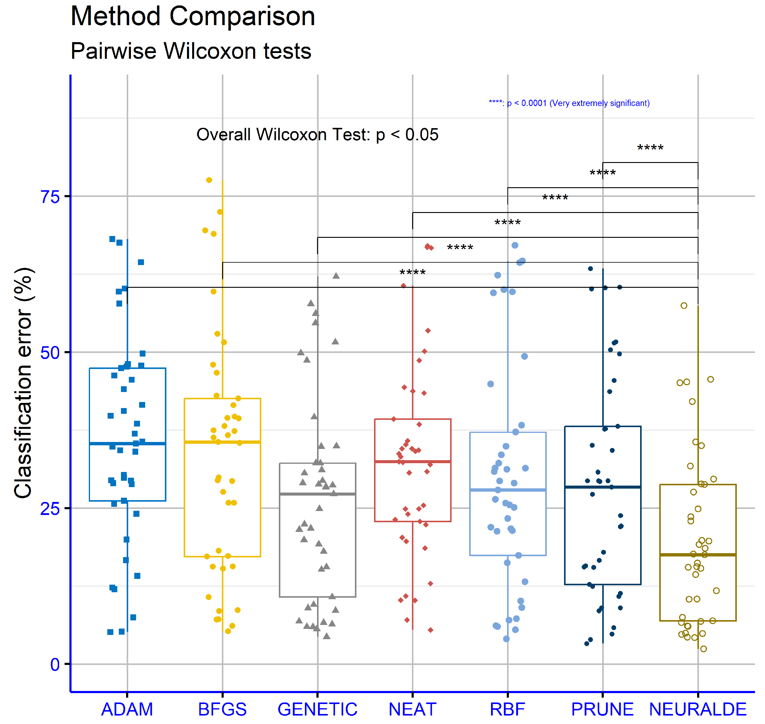
In Figure 2, the comparison of the proposed machine learning model NEURALDE with the other models for the classification datasets is illustrated, based on the values of the critical parameter p, which indicate the levels of statistical significance. The results show exceptionally low p-values, suggesting that the differences in the performance of NEURALDE compared to other models are not random and are statistically highly significant. Specifically, the comparison of NEURALDE with ADAM yielded p = 4.7 × ${10}^{-8}$, with BFGS p = 1 × ${10}^{-10}$, with GENETIC p = 2.9 × ${10}^{-9}$, with NEAT p = 2.3 × ${10}^{-10}$, with RBF p = 1.3 × ${10}^{-8}$, and with PRUNE p = 5.8 × ${10}^{-8}$. These values are well below the common thresholds of significance (p < 0.05: significant), indicating that the superiority of NEURALDE is statistically well founded. The results confirm the high efficiency of the proposed model compared to other machine learning methods, demonstrating its reliability and effectiveness in classification problems.

Similarly, the comparison of the proposed model with the others used to tackle the regression problems highlighted NEURALDE as the most efficient model. Specifically, the comparison of NEURALDE with ADAM yielded p = 0.00051, with BFGS p = 9.5 × ${10}^{-7}$, with GENETIC p = 0.0033, with NEAT p = 2.9 × ${10}^{-6}$, with RBF p = 0.0048, and with PRUNE p = 0.001. These values confirm the statistical significance of the differences, indicating that the superiority of NEURALDE in regression problems is well documented and not random, as shown in Figure 3.

Furthermore, the average classification error for the methods used in the experiments is presented in Figure 4, where the dynamics of the new technique are clearly depicted.

Likewise, the average regression error for all the techniques used is depicted in Figure 5.

Finally, the average execution time for all the methods involved in the conducted experiments regarding the classification datasets is graphically outlined in Figure 6.

As expected, the proposed method requires significantly more computation time than other method due to its complexity in the calculations and the requirement of the periodical application of a local optimization method.

3.2.1. Experiments with Differential Weight

Another series of experiments was carried out in order to determine the effect that the specific differential weight calculation mechanism has on the accuracy of the proposed technique. For this reason, the following methods were used for the calculation of the differential weight (parameter F):

• Denoted as MIGRANT in the experimental tables: In this case, the differential weight mechanism proposed in [110] was used.
• Denoted as ADAPTIVE in the experimental tables: This method used the differential weight calculation proposed in [111].
• Represented as RANDOM in the experimental tables: This method was the default method, suggested by Charilogis [59].

Table 4. Experimental results for the classification datasets using a list of proposed differential weight mechanisms found in the literature. Each column denotes a different weight mechanism and numbers in cells stand for the average classification error as measured on the corresponding test set.

Dataset	Migrant	Adaptive	Random
ALCOHOL	19.62%	18.44%	19.15%
AUSTRALIAN	14.77%	16.14%	15.31%
BALANCE	6.79%	6.94%	6.92%
BANDS	33.28%	35.42%	35.00%
CLEVELAND	45.74%	44.60%	45.07%
CIRCULAR	4.28%	4.34%	4.23%
DERMATOLOGY	11.41%	9.83%	10.38%
ECOLI	42.61%	47.51%	45.22%
HABERMAN	27.76%	28.35%	27.55%
HAYES-ROTH	35.92%	36.31%	35.59%
HEART	19.01%	17.29%	17.60%
HEARTATTACK	21.31%	20.28%	19.70%
HEPATITIS	56.37%	56.46%	57.46%
HOUSEVOTES	7.47%	7.54%	7.48%
IONOSPHERE	15.88%	16.40%	16.17%
LIVERDISORDER	32.56%	32.54%	31.72%
LYMOGRAPHY	26.52%	28.95%	28.86%
MAGIC	11.83%	11.28%	11.73%
MAMMOGRAPHIC	17.69%	17.44%	17.52%
PARKINSONS	13.28%	14.21%	14.32%
PAGE BLOCKS	5.48%	5.93%	6.04%
PHONEME	15.39%	15.17%	15.50%
PIMA	25.04%	23.28%	24.85%
POPFAILURES	5.55%	6.55%	6.09%
REGIONS2	26.26%	28.98%	28.77%
RING	21.04%	25.54%	22.90%
SAHEART	29.94%	29.80%	29.63%
SEGMENT	9.71%	15.99%	15.60%
SONAR	18.83%	18.93%	19.80%
SPAMBASE	5.87%	4.78%	4.95%
SPIRAL	41.36%	41.54%	42.06%
STATHEART	20.79%	19.32%	18.53%
STUDENT	4.36%	5.28%	4.86%
TAE	45.09%	44.78%	45.62%
TRANSFUSION	23.01%	24.51%	23.59%
WDBC	3.80%	4.55%	4.29%
WINE	8.22%	12.84%	10.39%
Z_F_S	7.16%	7.15%	6.81%
ZO_NF_S	4.19%	4.70%	4.73%
ZONF_S	2.47%	2.44%	2.41%
ZOO	5.23%	6.87%	6.63%
AVERAGE	19.34%	19.98%	19.78%

provides the performance of three differential weight computation methods (MIGRANT, ADAPTIVE, and RANDOM) on the series of classification datasets. The analysis reveals that the MIGRANT method achieves the smallest average error rate of 19.34%, indicating the best overall performance among the three methods. The RANDOM method follows closely, with an average error rate of 19.78%, while the ADAPTIVE method has the highest average error rate of 19.98%, suggesting that it is the least effective on average. Examining the individual datasets, MIGRANT is found to outperform the other methods in several cases. For example, in the HEART dataset, MIGRANT records an error rate of 19.01%, better than ADAPTIVE (17.29%) and RANDOM (17.60%). Similarly, in the MAGIC dataset, MIGRANT achieves a competitive error rate of 11.83%, which is close to RANDOM (11.73%) but higher than ADAPTIVE (11.28%). MIGRANT also has the lowest error in datasets such as ALCOHOL (19.62%), REGIONS2 (26.26%), and SPAMBASE (5.87%). ADAPTIVE demonstrates strong performance in specific datasets, achieving the lowest error rates in cases such as MAGIC (11.28%) and HEART (17.29%). However, in many datasets, it performs worse than MIGRANT or RANDOM, such as in SPAMBASE, where it records a lower error rate of 4.78% but is generally outperformed by the other critical datasets. The RANDOM method exhibits competitive performance in several datasets, achieving the lowest error rates in examples like ZOO (6.63%) and ZONF_S (2.41%). However, its performance fluctuates more significantly, with higher error rates in datasets such as HEARTATTACK (19.70%) and REGIONS2 (28.77%), where it is outperformed by MIGRANT and ADAPTIVE. Notable observations include cases where the error rates are very close across the methods, such as in datasets like CIRCULAR, where the differences are minimal (MIGRANT at 4.28%, ADAPTIVE at 4.34%, and RANDOM at 4.23%). In other cases, the differences are more pronounced, as in SEGMENT, where MIGRANT achieves 9.71%, significantly better than ADAPTIVE (15.99%) and RANDOM (15.60%). Overall, MIGRANT demonstrates the most consistent and robust performance across the datasets, with the lowest average error and competitive results in many individual datasets. RANDOM and ADAPTIVE have comparable average errors but show more variability in their performance.

The

Table 5. Experimental results for the regression datasets using a variety of differential weight methods. In every column, a different weight mechanism is depicted, and the numbers in the cells represent the average regression error as calculated on the corresponding test set.

Dataset	Migrant	Adaptive	Random
ABALONE	4.57	5.97	5.04
AIRFOIL	0.002	0.0011	0.0014
AUTO	45.37	18.89	16.21
BK	0.28	0.02	0.019
BL	0.007	0.019	0.016
BASEBALL	79.24	61.89	60.56
CONCRETE	0.0028	0.0029	0.003
DEE	0.27	0.35	0.35
FA	0.051	0.10	0.083
FRIEDMAN	1.66	1.32	1.22
HO	0.009	0.014	0.017
HOUSING	14.58	32.62	24.82
LASER	0.0026	0.0027	0.0026
LW	0.0189	0.044	0.021
MORTGAGE	0.43	0.93	0.54
PLASTIC	5.36	3.57	3.27
PY	0.12	0.14	0.11
QUAKE	0.038	0.041	0.042
SN	0.023	0.031	0.027
STOCK	15.94	3.58	3.40
TREASURY	0.70	1.24	1.021
AVERAGE	8.03	6.23	5.56

presents the performance of three differential weight computation methods (MIGRANT, ADAPTIVE, and RANDOM) on the regression datasets. The RANDOM method achieves the lowest average error, 5.56, making it the most effective overall. ADAPTIVE follows with an average error of 6.23, while MIGRANT exhibits the highest average error at 8.03, indicating the least effective performance. For specific datasets, RANDOM often outperforms the others. For instance, in the HOUSING dataset, it records an error of 24.82, lower than MIGRANT (14.58) and ADAPTIVE (32.62). Similarly, in the PLASTIC dataset, RANDOM achieves the smallest error of 3.27 compared to MIGRANT (5.36) and ADAPTIVE (3.57). RANDOM also shows superior performance in datasets like MORTGAGE (0.54) and STOCK (3.4). ADAPTIVE demonstrates strong performance in certain datasets, such as FRIEDMAN, where its error is 1.32, outperforming MIGRANT (1.66) and RANDOM (1.22). In the QUAKE dataset, ADAPTIVE records the lowest error of 0.041. However, its performance is noticeably weaker in other datasets, like HOUSING, where it registers the highest error of the three. MIGRANT outperforms in a few cases, such as the BL dataset, where its error is 0.007, significantly lower than ADAPTIVE (0.019) and RANDOM (0.016). However, it generally records higher errors in many datasets, such as AUTO (45.37) and BASEBALL (79.24), where the other methods perform better. In some cases, such as the LASER dataset, all methods perform similarly, with errors of 0.0026 for MIGRANT and RANDOM, and 0.0027 for ADAPTIVE. In the QUAKE dataset, the differences are also minimal, with RANDOM having the highest error (0.042), but very close to the others. Overall, RANDOM emerges as the most reliable and effective method, with the lowest average error and frequent superiority across the individual datasets. ADAPTIVE performs well in selected datasets but shows greater variability, while MIGRANT demonstrates the least effective performance, with higher errors across numerous datasets.

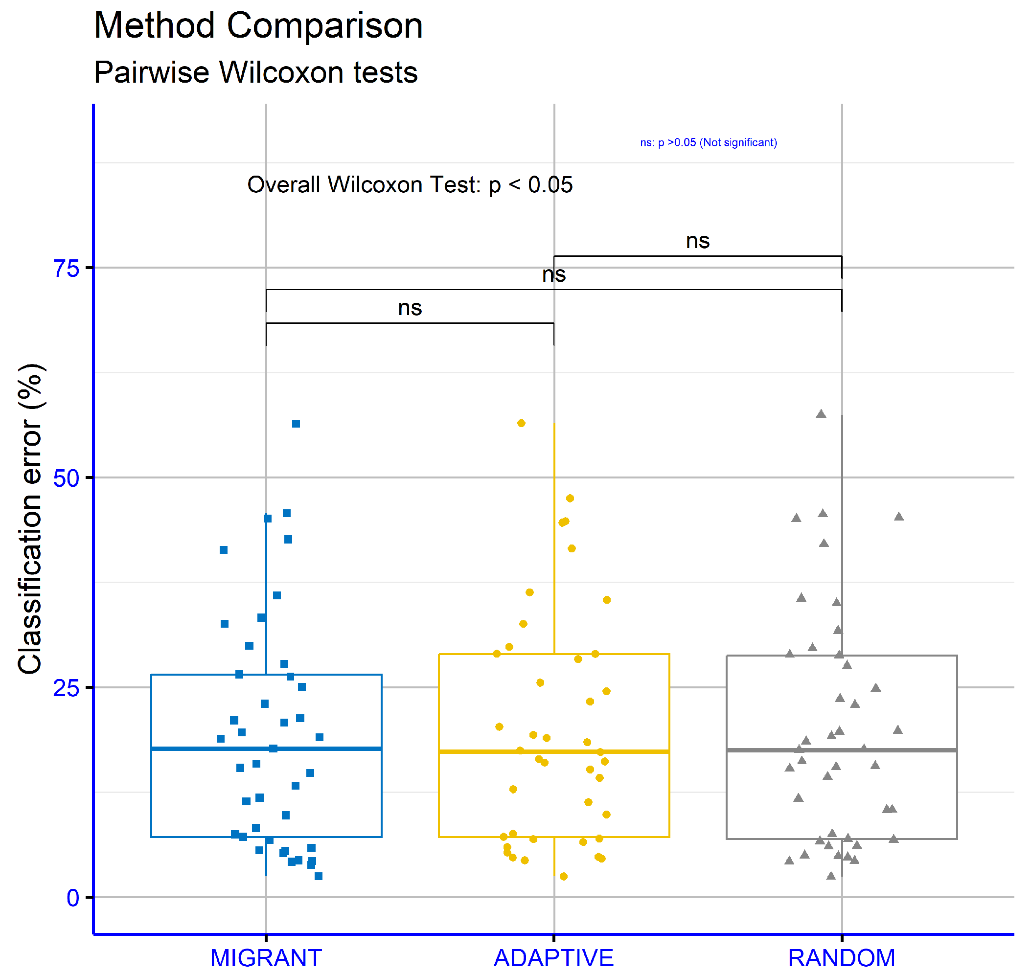
An analysis was conducted to compare different methods for computing differential weights in a proposed machine learning approach, focusing on classification error. The analysis employed the Wilcoxon Test for pairwise comparisons and was applied to the classification datasets. The goal was to examine whether statistically significant differences exist among the three approaches—MIGRANT, ADAPTIVE, and RANDOM (Figure 7). The results show that the comparison between MIGRANT and ADAPTIVE yielded a p-value of 0.085. Although this value suggests a trend of differentiation, it does not fall below the conventional significance threshold of 0.05, indicating that the difference is not statistically significant. Similarly, the comparison between MIGRANT and RANDOM produced a p-value of 0.064, which, while closer to significance, also does not meet the required threshold. Finally, the comparison between ADAPTIVE and RANDOM resulted in a p-value of 0.23, indicating no statistically significant difference between these two methods. Overall, the findings suggest that while there are indications of differences in behavior among the three approaches, none of these differences are statistically significant based on the data analyzed. This implies that the three methods for computing differential weights may be considered equivalent in terms of their impact on classification error, at least for the datasets used in this study.

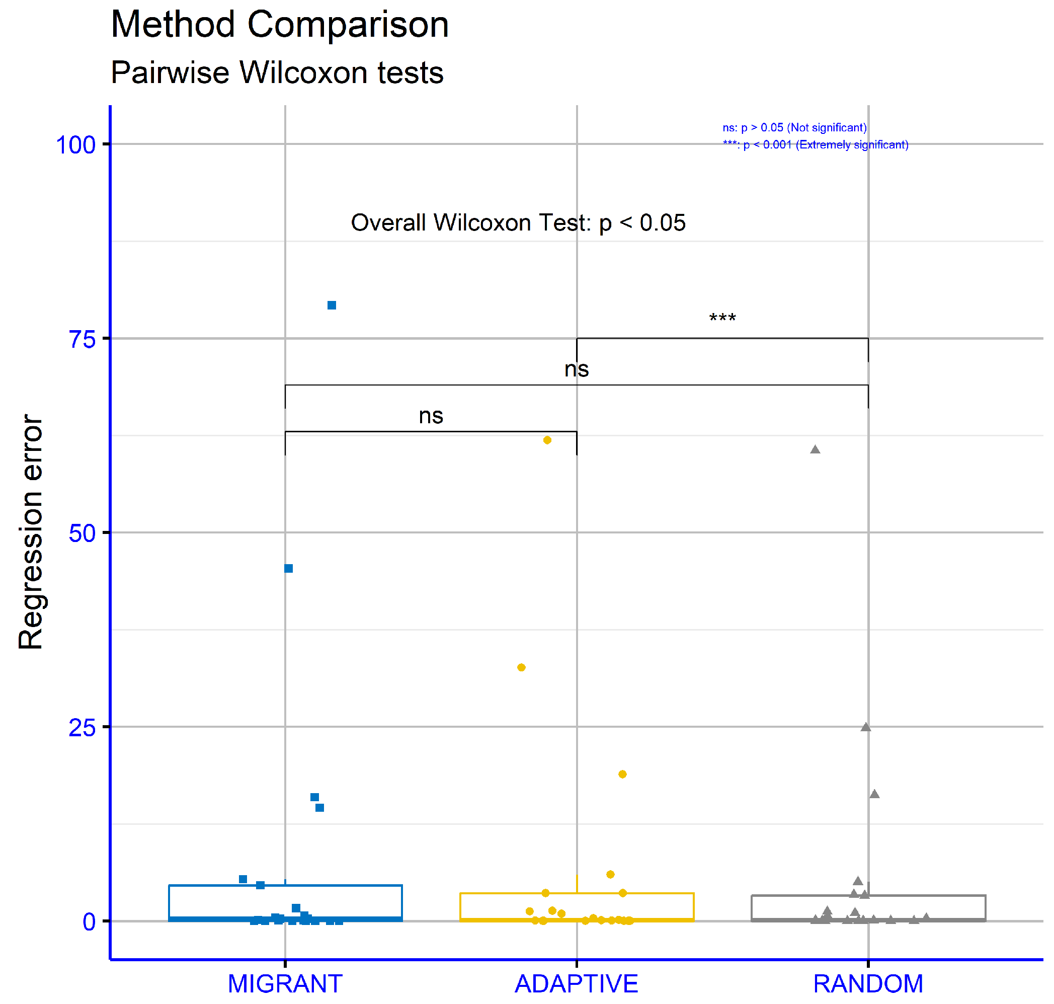
An analysis was conducted to compare the different methods for calculating differential weight in the proposed machine learning approach to the regression datasets. The Wilcoxon Test was used for pairwise comparison and applied across the series of regression datasets, with a focus on regression error. The aim was to determine the statistical significance of the observed differences between the methods (Figure 8). The results showed that the comparison between MIGRANT and ADAPTIVE yielded a p-value of 0.68, indicating no statistically significant difference between these two methods. Similarly, the comparison between MIGRANT and RANDOM resulted in a p-value of 0.9, confirming the absence of a statistically significant difference in this case as well. However, the comparison between ADAPTIVE and RANDOM produced a p-value of 0.00095, which is below the standard threshold for statistical significance (commonly 0.05). This suggests a statistically significant difference between these two approaches. Overall, the findings indicate that the MIGRANT and ADAPTIVE methods, as well as the MIGRANT and RANDOM methods, exhibit similar performance regarding regression error. In contrast, the ADAPTIVE method shows a clear and statistically significant differentiation from the RANDOM method.

3.2.2. Experiments with the Factor a

In the next series of experiments, the effect of the parameter a on the behavior of the method used on the classification and data fitting data was studied. In this series of experiments, different values of this parameter were studied. This parameter determines the allowable range of values within which the local minimization method can vary the parameters of the artificial neural network.

Table 6. Experimental results for the classification datasets using different values for the critical parameter a. In each column a different value for the critical parameter is used and numbers in cells represent the average classification error.

Dataset	$\mathit{a}=1.25$	$\mathit{a}=1.5$	$\mathit{a}=2$	$\mathit{a}=4$	$\mathit{a}=8$
ALCOHOL	21.49%	20.20%	19.15%	22.34%	19.86%
AUSTRALIAN	16.43%	16.89%	15.31%	15.90%	16.16%
BALANCE	7.49%	7.56%	6.92%	7.01%	7.16%
BANDS	34.88%	35.09%	35.00%	35.61%	35.01%
CLEVELAND	44.86%	46.08%	45.07%	44.67%	45.07%
CIRCULAR	4.17%	4.26%	4.23%	4.49%	4.61%
DERMATOLOGY	10.77%	10.65%	10.38%	9.87%	8.94%
ECOLI	44.13%	45.87%	45.22%	46.65%	47.46%
HABERMAN	27.24%	27.02%	27.55%	27.91%	28.40%
HAYES-ROTH	36.95%	36.46%	35.59%	35.82%	33.21%
HEART	17.43%	17.17%	17.60%	17.19%	17.19%
HEARTATTACK	19.50%	19.27%	19.70%	19.69%	19.69%
HEPATITIS	59.00%	57.38%	57.46%	60.21%	60.96%
HOUSEVOTES	7.07%	7.90%	7.48%	7.06%	7.07%
IONOSPHERE	14.24%	15.48%	16.17%	16.17%	15.43%
LIVERDISORDER	31.41%	31.59%	31.72%	32.23%	32.33%
LYMOGRAPHY	27.00%	27.07%	28.86%	27.57%	27.09%
MAGIC	12.18%	11.94%	11.73%	11.78%	12.25%
MAMMOGRAPHIC	17.42%	17.46%	17.52%	17.56%	17.54%
PARKINSONS	13.67%	13.40%	14.32%	14.19%	13.83%
PAGE BLOCKS	6.32%	6.28%	6.04%	5.83%	5.92%
PHONEME	16.07%	15.69%	15.50%	15.00%	15.00%
PIMA	24.59%	24.61%	24.85%	24.57%	24.79%
POPFAILURES	4.90%	5.28%	6.09%	7.50%	6.94%
REGIONS2	29.35%	28.94%	28.77%	28.79%	28.69%
RING	27.65%	26.97%	22.90%	23.92%	23.20%
SAHEART	29.33%	29.37%	29.63%	29.97%	30.47%
SEGMENT	18.18%	16.86%	15.60%	14.53%	14.27%
SONAR	19.27%	19.62%	19.80%	18.87%	20.16%
SPAMBASE	4.67%	5.07%	4.95%	5.00%	5.87%
SPIRAL	41.92%	41.76%	42.06%	41.49%	42.13%
STATHEART	19.22%	18.91%	18.53%	19.30%	20.22%
STUDENT	4.76%	4.55%	4.86%	5.84%	6.43%
TAE	47.54%	46.22%	45.62%	46.07%	44.38%
TRANSFUSION	23.74%	23.87%	23.59%	23.95%	24.15%
WDBC	4.48%	4.50%	4.29%	4.12%	4.14%
WINE	9.24%	9.67%	10.39%	10.39%	11.88%
Z_F_S	7.26%	6.67%	6.81%	6.64%	6.70%
ZO_NF_S	4.82%	4.91%	4.73%	4.42%	4.33%
ZONF_S	2.42%	2.55%	2.41%	2.68%	2.60%
ZOO	6.23%	6.93%	6.63%	7.07%	6.40%
AVERAGE	19.98%	19.95%	19.78%	20.00%	19.95%

presents the error percentages across the used classification datasets for different values of the parameter a (1.25, 1.5, 2, 4, and 8). The lowest overall average error is observed for $a=2$, with an average of 19.78%. This suggests that $a=2$ provides the most balanced performance across datasets. The other parameter values—1.25, 1.5, 4, and 8—yield average errors of 19.98%, 19.95%, 20.00%, and 19.95%, respectively. These results indicate that $a=2$ has a slight advantage in minimizing the overall error compared to the other values. For individual datasets, the performance varies depending on the parameter value. For example, in the ALCOHOL dataset, the smallest error is achieved at $a=2$ with 19.15%, while the other values result in slightly higher errors. Similarly, in the SEGMENT dataset, the error is minimized at $a=8$ with 14.27%. However, in datasets like SPIRAL, the errors across all parameter values are close, with no significant advantage for any specific value. In certain datasets, there is a clear trend in error reduction as the parameter value changes. For example, in the SEGMENT dataset, errors decrease consistently from $a=1.25$ to $a=8$. Conversely, in the ZOO dataset, the error decreases for lower values of a but increases again at higher values, indicating that performance is not always linear with changes in a. Some datasets exhibit minimal variability in performance across parameter values. For example, the error for the LIVERDISORDER dataset remains relatively stable, ranging from 31.41% to 32.33%. Similarly, the SPIRAL dataset shows little variation, with errors consistently around 42%. In other cases, specific parameter values consistently underperform. For instance, in the Z_F_S dataset, $a=1.5$ achieves the lowest error of 6.67%, while $a=2$ and $a=4$ result in slightly higher errors. Similarly, $a=8$ achieves the smallest error for certain datasets like SEGMENT but performs poorly for datasets like WINE. Overall, $a=2$ emerges as the most effective parameter value, yielding the smallest average error across datasets. While other values of a perform well in individual cases, their overall performance is less consistent.

Table 7. Experimental results for the regression datasets using different values for the critical parameter a. Each column contains experiments with different values for the critical parameter a. The numbers in the cells represent average regression error for the corresponding test set.

Dataset	$\mathit{a}=1.25$	$\mathit{a}=1.5$	$\mathit{a}=2$	$\mathit{a}=4$	$\mathit{a}=8$
ABALONE	4.36	4.66	5.04	7.63	8.84
AIRFOIL	0.002	0.0018	0.0014	0.0009	0.0007
AUTO	14.97	14.72	16.21	16.04	16.58
BK	0.02	0.02	0.019	0.11	0.21
BL	0.011	0.012	0.016	0.037	0.11
BASEBALL	57.67	58.42	60.56	67.70	72.37
CONCRETE	0.003	0.003	0.003	0.004	0.005
DEE	0.35	0.34	0.35	0.34	0.34
FA	0.067	0.056	0.083	0.24	0.42
FRIEDMAN	1.30	1.24	1.22	1.41	19.74
HO	0.011	0.012	0.017	0.043	0.17
HOUSING	28.09	25.93	24.82	22.86	26.45
LASER	0.0026	0.0025	0.0026	0.0027	0.0035
LW	0.019	0.019	0.021	0.073	0.77
MORTGAGE	0.50	0.45	0.54	0.75	0.62
PLASTIC	3.37	3.10	3.27	3.02	2.80
PY	0.12	0.13	0.11	0.09	0.09
QUAKE	0.04	0.041	0.042	0.048	0.096
SN	0.024	0.024	0.027	0.087	0.17
STOCK	2.82	3.13	3.40	3.21	5.42
TREASURY	0.87	0.81	1.021	1.06	1.06
AVERAGE	5.46	5.39	5.56	5.94	7.44

presents the error rates for the regression datasets across different values of the critical parameter a (1.25, 1.5, 2, 4, and 8). The lowest average error is observed for $a=1.5$, with an average of 5.39, suggesting that it offers the best overall performance. $a=1.25$ ranks second with an average of 5.46, and $a=2$ slightly higher at 5.56. The values $a=4$ and $a=8$ show a marked increase in errors, with averages of 5.94 and 7.44, respectively. This indicates that higher values of a are less effective compared to smaller ones. For individual datasets, performance varies with the value of a. For instance, in the AIRFOIL dataset, the error consistently decreases as a increases, with the smallest error (0.0007) observed at $a=8$. Conversely, in the FRIEDMAN dataset, the error rises sharply at $a=8$ (19.74), signaling a significant performance decline. In some datasets, such as BASEBALL, the error steadily increases with higher values of a rising from 57.67 at $a=1.25$ to 72.37 at $a=8$. In contrast, in the HOUSING dataset, the smallest error occurs at $a=4$ (22.86), although larger values like $a=8$ show only a slight increase. Certain datasets exhibit minimal sensitivity to changes in a. For example, in the LASER dataset, the errors remain almost constant regardless of the parameter value, ranging from 0.0025 to 0.0035. Similarly, in the DEE dataset, the errors are nearly identical across all values of a showing minimal variation. Interestingly, the PLASTIC dataset shows a gradual decrease in error from 3.37 at $a=1.25$ to 2.8 at $a=8$, indicating improved performance with increasing a. Conversely, in the STOCK dataset, the error increases significantly from 2.82 at $a=1.25$ to 5.42 at $a=8$. In conclusion, $a=1.5$ emerges as the optimal choice for minimizing overall error in this analysis. Higher values of a demonstrate reduced effectiveness, especially at $a=8$, where the average error rises notably. However, the results reveal that the impact of a varies by dataset, with some benefiting from smaller values and others exhibiting relative insensitivity to parameter changes.

In Figure 9, a comparison of the various values of the parameter a, which defines the bounds of the optimal values in the proposed machine learning method, is presented. The comparisons were conducted using the Wilcoxon Test across the series of used datasets to evaluate the classification error. The results indicate that the p-values for all pairwise comparisons between the different values of a are above the significance level of 0.05, suggesting no statistically significant differences. For instance, comparisons between $a=1.25$ and the other values (1.5, 2, 4, 8) yielded p-values ranging from 0.6 to 0.73, while comparisons between $a=1.5$ and other values (2, 4, 8) produced p-values ranging from 0.32 to 0.8. Similarly, comparisons between $a=2$ and higher values (4 and 8) resulted in p-values of 0.22 and 0.31, respectively, whereas the comparison between $a=4$ and $a=8$ yielded a p-value of 0.69. In conclusion, the results suggest that variations in the parameter a within the specified range do not lead to statistically significant differences in classification error, as all the p-values remain well above the conventional significance threshold. Therefore, the choice of a specific value for a is likely to have little or no impact on the method’s performance, based on the current data.

In Figure 10, the comparison of the different values of parameter a for the regression error is presented. The results show that statistically significant differences were observed in some comparisons, as the p-values were below the significance level of 0.05. For example, the comparison between $a=1.25$ and $a=4$ yielded p = 0.024, while between $a=1.25$ and $a=8$, p = 0.017 was observed. Similarly, the comparison between $a=1.5$ and $a=8$ resulted in p = 0.0021, indicating strong statistical significance. Conversely, some comparisons did not show statistically significant differences, as the p-values were above the significance level. For instance, the comparison between $a=2$ and $a=4$ yielded p = 0.22, while the comparison between $a=1.25$ and $a=2$ resulted in p = 0.15. In conclusion, the results suggest that the choice of parameter a affects the regression error in certain cases, with statistically significant differences primarily observed in comparisons between the smaller and larger values of the parameter. However, the differences are not always consistent and depend on the specific combinations of the values being compared.

3.2.3. Experiments with the Local Search Rate

In the last series of experiments, the effects of the execution rate of the local optimization methods were studied, focusing on values ranging from 0.25% to 2%.

Table 8. Experimental results for classification datasets using different values of local search rate $p_l$. In each column, a different value for the local search rate is used. Numbers in cells stand for the average classification error as measured on the corresponding test set.

Dataset	${\mathit{p}}_{\mathit{l}}=0.0025$	${\mathit{p}}_{\mathit{l}}=0.005$	${\mathit{p}}_{\mathit{l}}=0.01$	${\mathit{p}}_{\mathit{l}}=0.02$
ALCOHOL	19.15%	19.15%	21.81%	16.49%
AUSTRALIAN	17.93%	15.31%	14.17%	14.14%
BALANCE	7.44%	6.92%	6.63%	6.54%
BANDS	35.66%	35.00%	35.01%	34.44%
CLEVELAND	46.45%	45.07%	45.39%	45.32%
CIRCULAR	4.21%	4.23%	4.16%	4.31%
DERMATOLOGY	11.25%	10.38%	9.96%	9.07%
ECOLI	46.64%	45.22%	44.34%	44.66%
HABERMAN	27.99%	27.55%	27.66%	27.43%
HAYES-ROTH	36.33%	35.59%	34.03%	31.44%
HEART	17.05%	17.60%	17.35%	17.51%
HEARTATTACK	19.62%	19.70%	19.43%	20.37%
HEPATITIS	60.13%	57.46%	58.79%	60.34%
HOUSEVOTES	7.81%	7.48%	8.02%	7.47%
IONOSPHERE	15.52%	16.17%	16.33%	16.72%
LIVERDISORDER	31.92%	31.72%	32.06%	32.40%
LYMOGRAPHY	27.48%	28.86%	29.55%	29.98%
MAGIC	12.00%	11.73%	11.55%	11.57%
MAMMOGRAPHIC	17.23%	17.52%	17.34%	17.57%
PARKINSONS	14.70%	14.32%	13.39%	14.04%
PAGE BLOCKS	6.02%	6.04%	5.66%	5.76%
PHONEME	15.67%	15.50%	15.29%	15.04%
PIMA	25.52%	24.85%	24.63%	24.87%
POPFAILURES	5.46%	6.09%	6.30%	6.75%
REGIONS2	30.41%	28.77%	28.77%	28.02%
RING	27.01%	22.90%	24.05%	23.85%
SAHEART	29.91%	29.63%	29.54%	29.89%
SEGMENT	19.36%	15.60%	13.88%	11.70%
SONAR	19.62%	19.80%	20.38%	18.53%
SPAMBASE	6.30%	4.95%	5.43%	4.78%
SPIRAL	42.22%	42.06%	41.16%	40.35%
STATHEART	19.90%	18.53%	19.72%	20.47%
STUDENT	4.97%	4.86%	5.13%	5.01%
TAE	47.05%	45.62%	43.93%	45.05%
TRANSFUSION	24.41%	23.59%	23.11%	22.64%
WDBC	4.88%	4.29%	4.17%	4.07%
WINE	12.39%	10.39%	9.02%	8.41%
Z_F_S	7.11%	6.81%	6.26%	6.62%
ZO_NF_S	5.69%	4.73%	4.23%	3.93%
ZONF_S	2.45%	2.41%	2.45%	2.38%
ZOO	6.93%	6.63%	6.00%	6.50%
AVERAGE	20.48%	19.78%	19.66%	19.43%

provides the error rates for the classification datasets used under the different values of the periodic local search $p_l$ (0.0025, 0.005, 0.01, and 0.02). The analysis reveals that the lowest average error observed is $p_l=0.02$, with an error rate of 19.43%, suggesting that this value yields the best overall performance. This is closely followed by $p_l=0.01$, with an average error of 19.66%, and $p_l=0.005$ with 19.78%. The highest average error occurs at $p_l=0.0025$ with 20.48%, indicating comparatively poorer performance. Examining the individual datasets, the impact of $p_l$ appears to vary. For instance, in the ALCOHOL dataset, the smallest error is observed at $p_l=0.02$ with 16.49%, whereas larger values such as $p_l=0.01$ and $p_l=0.005$ result in higher errors (21.81% and 19.15%, respectively). Conversely, in the SEGMENT dataset, the error consistently decreases as $p_l$ increases, reaching its lowest value at $p_l=0.02$ with 11.70%. This trend is also evident in datasets such as SPAMBASE and WINE, where the errors decrease significantly with higher $p_l$ values. Some datasets exhibit minimal sensitivity to changes in $p_l$. For example, in the HEART and LIVERDISORDER datasets, the error rates remain relatively stable across all $p_l$ values, showing only marginal fluctuations. In other cases, such as CIRCULAR and HOUSEVOTES, the variations in error rates are similarly minor. However, certain datasets show exceptions to the general trend. For example, in the SONAR dataset, the error rate is lowest at $p_l=0.02$ with 18.53%, but higher $p_l$ values like $p_l=0.01$ produce increased errors (20.38%). Similarly, the REGIONS2 dataset achieves its best performance at $p_l=0.02$ with an error rate of 28.02%, but other $p_l$ values yield comparable results, such as 28.77% at both $p_l=0.005$ and $p_l=0.01$. The data suggest that higher $p_l$ values, particularly $p_l=0.02$, generally result in improved performance across most datasets. Nevertheless, the optimal $p_l$ value may vary depending on specific dataset characteristics, and some datasets show negligible or inconsistent responses to changes in $p_l$. Overall, $p_l=0.02$ is recommended for achieving the lowest average error.

Table 9. Experimental results for regression datasets using different values of the local search rate parameter $p_l$. The columns contain experiments with different values of the local search rate and the numbers in the cells represent average regression error for the corresponding test set.

Dataset	${\mathit{p}}_{\mathit{l}}=0.0025$	${\mathit{p}}_{\mathit{l}}=0.005$	${\mathit{p}}_{\mathit{l}}=0.01$	${\mathit{p}}_{\mathit{l}}=0.02$
ABALONE	4.48	5.04	5.27	4.93
AIRFOIL	0.0019	0.0014	0.0009	0.0006
AUTO	17.63	16.21	12.50	10.11
BK	0.027	0.019	0.03	0.029
BL	0.031	0.016	0.05	0.017
BASEBALL	63.05	60.56	62.57	71.93
CONCRETE	0.003	0.003	0.003	0.003
DEE	0.36	0.35	0.32	0.31
FA	0.056	0.083	0.066	0.091
FRIEDMAN	1.36	1.22	1.18	1.19
HO	0.015	0.017	0.017	0.016
HOUSING	32.72	24.82	18.24	14.02
LASER	0.0025	0.0026	0.0023	0.0024
LW	0.026	0.021	0.026	0.033
MORTGAGE	1.22	0.54	0.18	0.032
PLASTIC	3.61	3.27	2.66	2.43
PY	0.13	0.11	0.17	0.22
QUAKE	0.042	0.042	0.045	0.041
SN	0.025	0.027	0.027	0.025
STOCK	6.58	3.40	2.14	1.47
TREASURY	1.83	1.021	0.38	0.11
AVERAGE	6.34	5.56	5.04	5.10

presents error rates for the regression datasets used under the different values of the periodic local search $p_l$ (0.0025, 0.005, 0.01, and 0.02). The analysis indicates that the lowest average error is observed at $p_l=0.01$, with a value of 5.04, suggesting that this setting offers the best overall performance. This is followed by $p_l=0.02$, with an average error of 5.10, $p_l=0.005$ with 5.56, and $p_l=0.0025$ with 6.34, which has the highest average error and the poorest performance. Examining individual datasets reveals variations in the impact of different $p_l$ values. In the AUTO dataset, the error decreases steadily as $p_l$ increases, dropping from 17.63 at $p_l=0.0025$ to its lowest point of 10.11 at $p_l=0.02$. Similarly, in the HOUSING dataset, the error significantly reduces from 32.72 at $p_l=0.0025$ to 14.02 at $p_l=0.02$. This decreasing trend is also evident in other datasets, such as MORTGAGE, where the error falls from 1.22 at $p_l=0.0025$ to just 0.032 at $p_l=0.02$, and STOCK, where the error reduces from 6.58 to 1.47. In some datasets, the $p_l$ parameter has minimal impact. For instance, in the CONCRETE dataset, the error remains constant across all $p_l$ values at 0.003. Similar stability is observed in the QUAKE and SN datasets, where variations are minimal. However, some datasets exhibit less predictable trends. In the BASEBALL dataset, the error initially decreases from 63.05 at $p_l=0.0025$ to 60.56 at $p_l=0.005$ but then increases again to 71.93 at $p_l=0.02$. Similar inconsistent results are observed in the PY and BL datasets. Overall, the analysis suggests that $p_l=0.01$ delivers the best average performance. Nevertheless, the effect of the $p_l$ parameter varies across the datasets, with some benefiting more from higher or lower $p_l$ values.

In Figure 11, the pairwise comparisons using the Wilcoxon Test are presented to examine the impact of the different values of the local optimization parameter ($p_l$) on the proposed machine learning method, based on a series of well-known datasets, with the aim of evaluating the classification error. The Wilcoxon Test results showed that comparisons between $p_l=0.0025$ and $p_l=0.005$, $p_l=0.01$, and $p_l=0.02$ demonstrated statistically significant differences, as the p-values were lower than the significance level of 0.05. Specifically, the p-value for the comparison between $p_l=0.0025$ and $p_l=0.005$ was 0.0001, between $p_l=0.0025$ and $p_l=0.01$ was 0.00034, and between $p_l=0.0025$ and $p_l=0.02$ was 0.00048. Conversely, the comparisons between $p_l=0.005$ and $p_l=0.01$, as well as between $p_l=0.01$ and $p_l=0.02$, did not show statistically significant differences, with p-values of 0.21 and 0.57, respectively. The comparison between $p_l=0.005$ and $p_l=0.02$ yielded a p-value of 0.052, indicating a marginal lack of significance. Overall, the results suggest that the choice of the pl parameter value affects the classification error primarily in comparisons involving the value $p_l=0.0025$, while the other comparisons do not exhibit clear statistically significant differences.

In Figure 12, the regression error for the different values of the periodic local search parameter is presented. In the comparison between $p_l=0.0025$ and $p_l=0.005$, the p-value was 0.011, indicating a statistically significant difference, as it is below the significance level of 0.05. In contrast, the comparisons between $p_l=0.0025$ and $p_l=0.01$, between $p_l=0.0025$ and $p_l=0.02$, between $p_l=0.005$ and $p_l=0.01$, and between $p_l=0.005$ and $p_l=0.02$ did not show statistically significant differences, with p-values of 0.12, 0.18, 0.22, and 0.097, respectively, all of which are above the significance level of 0.05. Finally, the comparison between $p_l=0.01$ and $p_l=0.02$ yielded a p-value of 0.086, which is close to but above the significance level of 0.05, suggesting borderline non-significance. Overall, the results indicate that only the comparison between $p_l=0.0025$ and $p_l=0.005$ showed a statistically significant difference, while the remaining comparisons did not present clear statistically significant differences.

3.2.4. Experiments with the Local Search Method

Another test was conducted, where the local optimization method of the proposed technique was altered. In this test, two local optimization methods—Limited Memory BFGS (LBFGS) [112] and Adam [17]—were used and the results were compared against those obtained by the application of the BFGS local optimization methods. The experimental results for the classification datasets are depicted in

Table 10. Experimental results for the classification datasets using different local search methods for the classification datasets. Numbers in cells stand for the average classification error as measured on the corresponding test set.

Dataset	Bfgs	Lbfgs	Adam
ALCOHOL	19.15%	22.76%	19.36%
AUSTRALIAN	15.31%	21.80%	31.19%
BALANCE	6.92%	7.29%	8.08%
BANDS	35.00%	35.58%	35.72%
CLEVELAND	45.07%	43.76%	44.76%
CIRCULAR	4.23%	4.29%	4.52%
DERMATOLOGY	10.38%	9.09%	11.34%
ECOLI	45.22%	46.43%	51.36%
HABERMAN	27.55%	27.17%	27.63%
HAYES-ROTH	35.59%	37.00%	35.38%
HEART	17.60%	15.93%	20.59%
HEARTATTACK	19.70%	18.57%	21.80%
HEPATITIS	57.46%	56.50%	57.25%
HOUSEVOTES	7.48%	7.74%	5.39%
IONOSPHERE	16.17%	16.57%	11.77%
LIVERDISORDER	31.72%	32.29%	33.06%
LYMOGRAPHY	28.86%	27.93%	23.57%
MAGIC	11.73%	11.83%	12.72%
MAMMOGRAPHIC	17.52%	16.76%	17.13%
PARKINSONS	14.32%	13.58%	15.42%
PAGE BLOCKS	6.04%	5.80%	6.78%
PHONEME	15.50%	15.36%	16.93%
PIMA	24.85%	24.24%	30.67%
POPFAILURES	6.09%	6.74%	4.58%
REGIONS2	28.77%	29.89%	29.58%
RING	22.90%	23.64%	25.66%
SAHEART	29.63%	28.70%	32.18%
SEGMENT	15.60%	19.46%	27.47%
SONAR	19.80%	19.35%	18.65%
SPAMBASE	4.95%	4.78%	3.91%
SPIRAL	42.06%	41.74%	42.84%
STATHEART	18.53%	17.59%	20.22%
STUDENT	4.86%	5.23%	3.82%
TAE	45.62%	47.20%	51.20%
TRANSFUSION	23.59%	24.32%	25.06%
WDBC	4.29%	4.18%	6.00%
WINE	10.39%	10.06%	14.82%
Z_F_S	6.81%	7.10%	11.03%
ZO_NF_S	4.73%	5.34%	9.72%
ZONF_S	2.41%	2.74%	3.36%
ZOO	6.63%	6.20%	8.00%
AVERAGE	19.78%	20.06%	21.48%

, while the experimental results for the regression datasets are shown in

Table 11. Experimental results for the regression datasets using different local search methods.

Dataset	Bfgs	Lbfgs	Adam
ABALONE	5.04	4.48	4.38
AIRFOIL	0.0014	0.0024	0.0031
AUTO	16.21	19.60	20.70
BK	0.019	0.017	0.018
BL	0.016	0.010	0.024
BASEBALL	60.56	49.78	78.73
CONCRETE	0.003	0.003	0.003
DEE	0.35	0.30	0.36
FA	0.083	0.020	0.022
FRIEDMAN	1.22	1.23	2.29
HO	0.017	0.009	0.02
HOUSING	24.82	35.57	47.63
LASER	0.0026	0.0027	0.0025
LW	0.021	0.012	0.015
MORTGAGE	0.54	1.54	2.01
PLASTIC	3.27	2.53	3.40
PY	0.11	0.09	0.04
QUAKE	0.042	0.044	0.047
SN	0.027	0.032	0.024
STOCK	3.40	8.90	11.27
TREASURY	1.021	2.43	2.60
AVERAGE	5.56	6.03	8.27

.

The analysis of Table 10 regarding the local search methods BFGS, LBFGS, and ADAM for the NEURALDE model presents their performance on the classification datasets, with the values representing error percentages. According to the results, the BFGS method achieves the lowest average error rate at 19.78%, followed by LBFGS with 20.06% and ADAM with 21.48%. This highlights the relative superiority of BFGS in minimizing error compared to the other methods. When analyzing the individual datasets, BFGS records the lowest error rates in several cases. For instance, in the HOUSEVOTES dataset, both BFGS and LBFGS yield similar results, while ADAM shows the lowest error at 5.39%. In the SPAMBASE dataset, ADAM outperforms the others with an error rate of 3.91%, compared to 4.95% and 4.78% for BFGS and LBFGS, respectively. Similarly, in the STUDENT dataset, ADAM performs best with the lowest error at 3.82%. However, in datasets like SEGMENT, BFGS excels with a significantly lower error of 15.60% compared to 19.46% for LBFGS and 27.47% for ADAM. Notable differences are observed in datasets such as DERMATOLOGY, where LBFGS records the lowest error at 9.09%, compared to 10.38% for BFGS and 11.34% for ADAM. In the MAGIC dataset, BFGS and LBFGS deliver comparable performance, with error rates of 11.73% and 11.83%, respectively, while ADAM presents a higher error of 12.72%. Similarly, in the CIRCULAR dataset, BFGS achieves the lowest error at 4.23%, closely followed by LBFGS at 4.29%, and ADAM at 4.52%. Overall, BFGS demonstrates superior performance in most cases, maintaining the lowest variation in error rates and achieving the smallest average error. However, LBFGS delivers competitive results with a slightly higher average error and outperforms in specific datasets like DERMATOLOGY. While ADAM records lower error rates in isolated datasets such as SPAMBASE and STUDENT, it exhibits a higher overall error, indicating greater variability in its performance. In conclusion, the BFGS method emerges as the most efficient overall, while LBFGS offers consistently competitive performance. ADAM shows advantages in certain datasets but has a higher overall average error rate.

The evaluation presented in Table 11 highlights the performance of the local search methods—BFGS, LBFGS, and ADAM—applied to the regression datasets within the NEURALDE model. The reported values correspond to absolute errors. Among the three methods, BFGS achieves the lowest mean error of 5.56, demonstrating a clear advantage over LBFGS and ADAM, which have mean errors of 6.03 and 8.27, respectively. Examining individual datasets, BFGS achieves superior results in several instances. For example, in the AIRFOIL dataset, it records the smallest error at 0.0014, while LBFGS and ADAM show slightly higher errors of 0.0024 and 0.0031, respectively. On the other hand, LBFGS outperforms in the BASEBALL dataset, achieving the lowest error at 49.78, compared to 60.56 for BFGS and 78.73 for ADAM. Similarly, LBFGS demonstrates the best performance in the BL dataset with an error of 0.01, outperforming BFGS and ADAM, which exhibit errors of 0.016 and 0.024, respectively. In the PLASTIC dataset, LBFGS again achieves the smallest error at 2.53, followed by BFGS with 3.27 and ADAM with 3.4. Conversely, in the MORTGAGE dataset, BFGS performs best, with an error of 0.54, while LBFGS and ADAM display larger errors of 1.54 and 2.01. In the STOCK dataset, BFGS also demonstrates superior performance, recording the lowest error at 3.4, whereas LBFGS and ADAM show significantly higher errors of 8.9 and 11.27, respectively. Certain datasets exhibit negligible differences in performance among the methods. For instance, in the CONCRETE dataset, all three methods produce identical errors of 0.003. Similarly, in the LASER dataset, the errors are nearly identical, with ADAM achieving 0.0025, BFGS achieving 0.0026, and LBFGS achieving 0.0027. Overall, BFGS emerges as the most effective method, delivering the lowest average error and consistently strong results across numerous datasets. LBFGS, while slightly less efficient on average, demonstrates competitive performance in specific datasets such as BASEBALL, BL, and PLASTIC. ADAM, though occasionally effective, as observed in datasets like LASER, shows greater variability and a higher mean error, limiting its overall reliability. In conclusion, BFGS stands out as the most robust and dependable method, with LBFGS showing significant potential in select contexts.

In Figure 13, the critical parameter p, which indicates the level of statistical significance, showed no statistically significant difference between the BFGS and LBFGS methods, with p = 0.78. This high value does not meet the common significance threshold (p < 0.05). In contrast, the comparison between BFGS and ADAM revealed a statistically significant difference, with p = 0.0017, indicating clear differentiation between the two methods. Similarly, the comparison between LBFGS and ADAM recorded p = 0.0031, which is also below the significance level, proving that the two methods exhibit statistically significant differences in classification error performance.

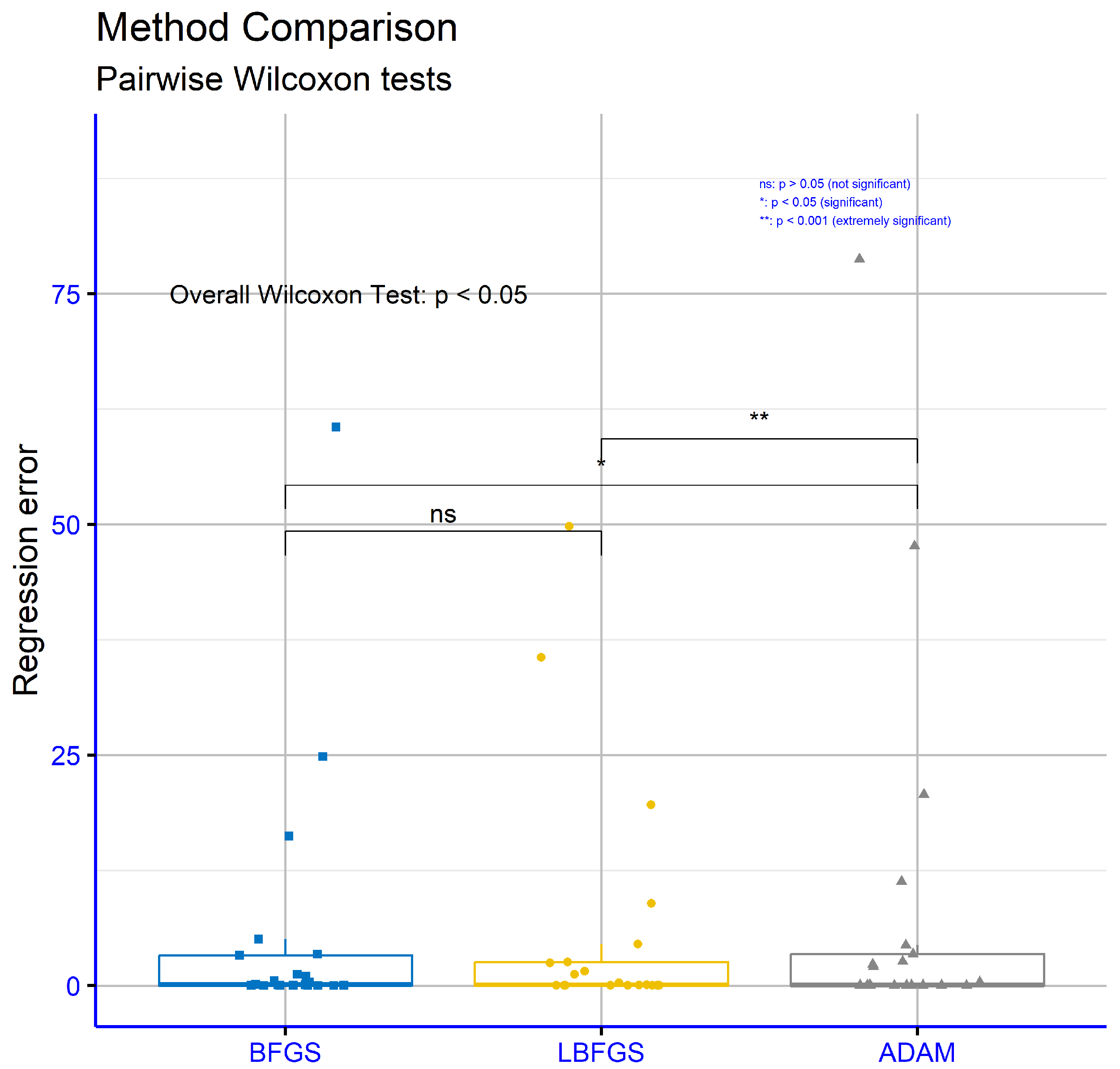
In Figure 14, the results showed that the BFGS and LBFGS methods have no statistically significant difference, with p = 1.0, suggesting that the two methods perform essentially the same regarding regression error. However, the comparison between BFGS and ADAM resulted in p = 0.037, which is below the 0.05 threshold, highlighting a statistically significant difference favoring BFGS. Lastly, the comparison between LBFGS and ADAM recorded p = 0.0054, confirming a statistically significant differentiation between these two methods as well. In summary, the results of the Wilcoxon Test demonstrate that BFGS and LBFGS have comparable performances in regression error, while they do not exhibit statistically significant differences in classification error. On the other hand, the differences between ADAM and the other two methods (BFGS and LBFGS) are statistically significant in both cases, indicating that ADAM shows distinct performance characteristics in both classification and regression error.

3.3. Summary of Experimental Results

In conclusion, the analysis conducted on the data within the tables and figures of the study reveals significant findings regarding the performance of different machine learning models and parameters. Below is a summary of the key points of the statistical analysis. The analysis primarily focuses on the NEURALDE model and its performance compared to the other optimization models (ADAM, BFGS, GENETIC, NEAT, RBF). Non-parametric statistical tests such as the Wilcoxon Test were utilized, which are suitable for data that do not follow a normal distribution. The statistically significant differences observed ($p<0.05$) highlight the consistent superiority of NEURALDE in most cases. Specifically, the model achieved the lowest average error rate in both classification (19.78%) and regression problems (average error of 5.56), consistently outperforming its competitors. Similarly, in the tables comparing the different weight computation methods (MIGRANT, ADAPTIVE, RANDOM), MIGRANT demonstrated the best performance in classifications, with an average error of 19.34%, while RANDOM excelled in regressions, with an average error of 5.56. The deviations among these methods warrant further investigation regarding error variability across datasets. In the parameter analysis, the a value (range of optimal values) and $p_l$ (periodic local optimization parameter) appear to influence performance differently depending on the context. For example, the a parameter with a value of 2 achieved the lowest average error in classifications, while for regressions, a value of 1.5 was most effective. Similarly, for $p_l$, the value of 0.02 consistently showed better performance in classifications, whereas 0.01 proved more effective for regressions. In summary, the results underline the importance of selecting the appropriate model and parameters based on the characteristics of the data. NEURALDE stands out as the most robust and efficient model, significantly outperforming its competitors. The specific parameters and methods affect overall performance and should be carefully evaluated to optimize the system.

4. Conclusions

The study focuses on the development and evaluation of the NEURALDE method, an innovative approach to optimizing neural network training based on differential evolution (DE). The results demonstrate that NEURALDE outperforms traditional optimization techniques such as ADAM, BFGS, GENETIC, NEAT, and RBF in both classification and regression tasks. Across a wide range of datasets, NEURALDE consistently achieved the lowest error rates, confirming its robustness and efficiency. Statistical analyses, including the Wilcoxon Test, were used to validate the significance of the differences between NEURALDE and the other methods. The extremely low p-values indicate that the observed differences are not random but reflect the actual superiority of NEURALDE. Furthermore, the method proved resilient to common neural network training challenges, such as overfitting and entrapment in the local minima.

NEURALDE is established as a reliable and high-performance optimization method for machine learning applications. Its exceptional performance in both classification and regression, combined with statistical validation of its superiority, positions it as a strong contender for broader adoption in various machine learning applications. The method is particularly useful for complex datasets or scenarios where traditional approaches fail to deliver satisfactory results.

This study opens multiple avenues for further research. Firstly, exploring the scalability of NEURALDE on larger and more diverse datasets could provide valuable insights into its generalizability and practical utility. Incorporating adaptive mechanisms within the differential evolution framework is another promising direction, as it could dynamically adjust parameters based on dataset characteristics, further enhancing the method’s performance. Another interesting avenue is applying NEURALDE to unsupervised learning tasks, such as clustering, to evaluate its adaptability across different machine learning paradigms. Furthermore, integrating NEURALDE with cutting-edge techniques like transfer learning and reinforcement learning could unlock new potential, particularly for real-time applications and complex decision-making environments. Future research could also focus on reducing the computational cost of the method to make it more accessible for large-scale problems. Overall, NEURALDE provides a robust foundation for further improvements and extensions, aiming to establish it as a key optimization method in machine learning.

However, the proposed technique exhibits significantly increased execution time compared to the original training algorithm due to the periodic use of the differential evolution technique. These problems can be circumvented by using parallel processing techniques such as the MPI interface [113] and the OpenMP programming library [114]. Also, parallel approaches to the differential evolution [115,116] technique could also be incorporated to significantly reduce the required computing time.