Technical Systems Under Stress: New Lifespan Models and Calculation Methods

Abstract

Technical systems, which form the basis of modern technology, are structures designed to achieve a specific purpose by bringing together different components. In this respect, they have a wide field of study. Our study is aimed at the general evaluation of technical systems operating under stress. The reliability of technical systems is directly related to order statistics. Therefore, first of all, when the moment of failure is observed, a life time distribution is proposed, which is revised at each moment of failure. Secondly, a new expected value operator is proposed. Thanks to this operator, the average working time under stress can be calculated easily without deforming the working time distribution. Finally, the differential structure of the stress factor is examined in detail, and two different differential equations and solutions are proposed depending on the working time distribution. The numerical calculations presented in the study include detailed information on the applications of the proposed methods.

1. Introduction

It is obvious how important research and development studies are in a significant part of industrial production. Standardizing the important features of a manufactured product is an important reason for consumer preference. The first standard feature of the product in production is the average working time, or simply the life expectancy of the product. This feature is calculated under ideal conditions for a product leaving production and the warranty period of the product is determined accordingly. However, it is observed that the lifespan of the product is shorter than expected in environments where ideal conditions are not met. This situation, explained with a short example, has made it necessary to examine systems operating under stress and has become an important area of investigation in the recent literature. In his review, Mazzanti, G. [1] presented an important method for estimating the lifespan of high voltage cables operating under high electro thermal stress due to voltage and load cycles. Thermal transients as a result of cyclic current changes place significant stress on cable insulation. Thanks to this study, the average life expectancy of cable insulation under specified stress can be calculated. Pfanz, H. et al. [2] investigated the lifespan of spruce tree needle leaves in intense air pollution and sparse forest tissue. Unlike species that live in their natural environment, conifers show a lower lifespan under stress caused by weather and environmental conditions. Chandra, A. et al. [3] investigated the effects of mechanical stress and chemical conditions on the lifespan of hip implants. Determining the lifespan of the implant under the stress caused by different materials, processes and living conditions provides the basis for the optimal use of materials and methods used in this field. It is possible to increase such research examples. Although the research areas of the three examples given here are quite different from each other, their purposes are the same. This reveals the importance of investigating systems operating under stress. The examples given above are usually in the form of the lifetime of a single component. However, technical systems are more complex. More detailed analysis is needed to examine these structures. Let us talk a little bit about these methods at this stage. A similar field of study that investigates the effect of stress on the system is stress–strength models. The results obtained from stress–resilience models cannot be directly applied to systems operating under stress. Stress–resilience models are rather a comparison of the effect of the existing stress with the resilience of the system. Briefly, with X being a variable indicating the resilience of the system and Y being a variable indicating the strength of the stress, the stress–strength model is concerned with the probability of the event {X > Y}. In the stress–strength model, the reliability of the system is expressed by this probability:

R = P{X > Y}.

Here, the situation where the system’s resistance is greater than the stress is shown by the event {X > Y}. The probability of this event is the reliability of the technical system operating under stress.

However, how to define system resilience in the stress–strength model is very important. The lifetime of a system can be perceived as the resilience of the system. However, since the lifetime of the system cannot be compared with the amount of stress in units, the {X > Y} event becomes meaningless. For this phenomenon to be measurable, the unit of system resilience must be compatible with the unit of stress. Since system reliability is a percentage expression, it is natural to express it with probability. In this respect, the event expressing reliability must be meaningful.

Important studies on the stress–strength model can be found in the literature. In his book on this subject, Johnson, R. A. [4] emphasized that the stress conditions of the working environment should also be taken into account when determining the reliability of the component. The importance of modeling the adverse conditions that may arise during the operation of the system, or stress in short, is quite high. In the model, both stress and strength are treated as random variables. Reliability is defined as the probability that the system is strong enough to overcome the stress. In this respect, the stress–strength model has many applications in civil, mechanical and aerospace engineering. Eryılmaz, S. [5] presented a multi-state stress–strength model by leveling the two-state structure of the stress–strength model. This leveling was based on the difference between stress and strength. Gökdere, G. and Bugatekin, A. [6] stated that the reliability formula derived for the m-consecutive-k-out-of-n: F (m/C/k/n: F) system requires less computation time than the m/C/k/n: F system formula that is currently in use.

When we look at the literature, the probability of the event {Y < X} assumed between stress and strength is the decision criterion in stress–strength models. The stress effect is usually applied to the distribution of the working time. Our study aims to gather stress–strength models from accessible sources in the literature under a single roof. Therefore, our study primarily aims to place stress on a mathematical structure in general. In the second part that follows, stress is considered as a random variable and its geometric and differential structure is tried to be examined in detail.

The study is basically divided into three categories. The first is the structure and adaptation of order statistics used for system reliability. This situation is presented in Section 2.1 “First Critical Approach: Distribution of Life Time of System Components” and supported by simulation study. The second is the study of average life time of a system operating under stress, presented in Section “Third Critical Approach: Average Time for System on Renovation or Repair”. The third part is the geometric structure and differential properties of the stress factor, presented in Section 5 “Geometric Interpretation of the Stress Factor” and presented in Section 6 “Fourth Critical Approach: Differential Interpretation of the Stress Factor”. In Section 5, the geometric structure of the general stress factor is constructed and an important application is shown with the help of some random variables. In Section 6, the solutions are examined using two different differential equations.

In particular, the differential examination of the stress variable is a first in the literature. The obtained results are included in the whole study. At this stage, two linear differential equations are presented for stress. First, when the stress factor cannot be measured, the solution obtained from the system’s working time gives us the stress variable. In the second equation, a solution can be found that allows the system’s working time to be obtained when the stress variable can be measured.

2. Materials and Methods

2.1. Investigation of the Technical System Under Stress

When the stress effect in the environment is to be reflected in the operation of the system, there can be three different situations. In the first case, the stress effect is reflected in the variable representing the lifetime of the system [4],

$$X^{*}=YX,$$

where$Y$ is the effect of stress, X is the ideal lifetime of the system and $X^{*}$ is the lifetime of the system under the existing stress. Naturally, since the stress effect in the environment will shorten the ideal lifetime of the system, it is chosen as $0\le Y\le 1$. There are alternative cases of this choice. For example, when $U~Exp\left(\mu \right)$ distribution, the variable $Y$ can be chosen as follows [4],

$$Y={\displaystyle \frac{1}{1+U}}.$$

Here, when $U=0$, in the absence of stress, $Y=1$ and $X^{*}=X$, and when $U\to \infty , Y=0$ and $X^{*}=0$. These two properties are essential for systems studied under stress. Estimation of the distribution parameter for a stress variable taken from its distribution may not always yield results according to conventional estimation methods. This is still an important area of investigation in the literature. Let us briefly note here that the choice of the variable $Y$ should be chosen depending on the robustness of the system under stress and the variability of the stress effect. For sensitive changes in the range $0\le Y\le 1$, the Mittag–Leffler function can be used (Mittag–Leffler, G. M.) [7].

In the second case, the stress effect can be reflected in the reliability function of the system. In this case, the reliability of the system under stress is $R^{*}\left(t\right)=YPr\left\{X>t\right\}=YR\left(t\right).$In this case, the choice of the variable $Y$ is the same as in the first case. However, here

$$R^{*}\left(t\right)=e\left(t\right)+YR\left(t\right).$$

It should be noted that the regression equation of the form of the regression equation is adhered to. In the third case, the stress effect can be reflected in the time between failures. This is more applicable to the analysis of multi-component systems or systems operating under the repair principle. In the literature, there is almost no analysis of system reliability by considering the time between successive failures. Triantafyllou analyzed the structure of threshold reliability systems composed of different types of independent components and derived explicit expressions for reliability functions, mean time to failure, and Birnbaum importance measures [8]. The reason for the scarcity of such studies in the literature is that the system is mostly represented by the lifetime and the system cannot always be represented by the time between successive failures. If the stress effect is to be reflected in the time between successive failures, the following successive equation should be considered,

$$A_{k+1}\left(t\right)=e\left(t\right)+\underset{0}{\overset{\infty }{{\displaystyle \int }}}{A}_k\left(t/y\right)d{F}_Y\left(t\right).$$

Here, $A_k$ denotes the probability that the time between two consecutive distur-bances is greater than $t$ time. It should be noted that the above equation is also in the form of a regression equation. The most important point to be emphasized here is that the stress model, which is considered in the third category, utilizes the distribution of the time elapsed between failures, not the operating times of the components. In some publications in the literature, the Markov process representing the technical system has taken the time between failures as exponential, although the running times of the components are exponential Gökdere, G. et al. [9]. This important paradox arises from the fact that the sequential differences of the order statistics taken from the exponential distribution are also different from the exponential, but behave close to the exponential.

2.2. First Critical Approach: Distribution of Life Time of System Components

The distribution of the lifetime of the system components is the most important information for calculating the reliability of the system. In this respect, it is very important to choose the distribution that represents the component’s lifetime. The most basic of the distributions used for lifetime is the exponential distribution. In Exp(λ) distribution, the average lifetime is $1/\lambda$ and for small values of this parameter, the lifetime is large, and for large values of this parameter, the lifetime is small. In many analytical calculations, it is natural to choose the exponential distribution as the life distribution because of its convenience. However, there are some disadvantages in using the exponential distribution as a life distribution. The most important one is the memorylessness property of the exponential distribution. Briefly, the memoryless property means that if the component is known to be running at any time; this moment is taken as the beginning of the running time. The memoryless property deals with conditional events. Since the condition is directly reflected in the variable of the distribution function, it facilitates many calculations. However, it is inherently not always correct to consider a component in a technical system as a component whose operating time does not depend on the moment of observation and which starts working from scratch after that moment. This property depends on the structure of the running component. The density function in exponential form at the moment of observation $c>0$ is expressed as follows,

$$f\left(t\right)=\lambda \exp \left(-\lambda \left(t-c\right)\right), t\ge c, \lambda >0, c>0.$$

(1)

The lifetime starts at $c>0$ and the average lifetime is $c+1/\lambda .$These properties are very convenient for analyzing the lifetime of a system. The probability that a system known to be running at any instant $t\ge 0$ will run for $h\ge 0$ time after this instant depends only on the time $h$. Since it is independent of the past operating time of the system, it does not add any obsolescence or wear and tear property to the operating system. In systems operating under stress, it is very difficult to reflect the effect of stress in the parameter $\lambda =\lambda \left(t\right)$. For these reasons, in order to reflect the effect of stress in the $\lambda$ parameter, the stress variable should have a multiplier. This situation can be clearly seen in two studies in the literature, Eryılmaz, S. [5] and Gökdere, G. et al. [9].

In order to eliminate such errors, the distribution representing the lifetime must be carefully chosen or deformed from a distribution known to be appropriate. Let us illustrate this by deforming the lifetime from an exponential distribution for a technical system consisting of two components connected in parallel.

In a two-component parallel connected system, the first moment of disturbance cannot be known until the disturbance occurs. The second moment of disturbance is also the moment of failure of the system. Let us denote the moment of failure by $c>0$. Accordingly, the distribution function of the lifetime of both components of the system can be taken as follows,

$$F\left(t\right)=\left\{\begin{array}{c}{\displaystyle \frac{{\alpha }_1}{1-\exp \left(-{\lambda }_{1}c\right)}}(1-\exp \left(-{\lambda }_{1}t\right)) : 0<t<c\\ 1-{\alpha }_2\exp \left(-{\lambda }_2\left(t-c\right)\right) : t\ge c \end{array} \right.$$

(2)

Here, ${\alpha }_1=Pr\left\{t<c\right\}$ satisfies the equality ${\alpha }_1+{\alpha }_2=1$. It is also a distribution function deformed from this exponential distribution. This function is very important for the calculation of system reliability when component lifetimes are exponential. At first glance, the distribution function given by (2) may be perceived as a structure incompatible with the past literature. However, the distribution function proposed by (2) is actually a piecewise written form of the following distribution function,

$$\left(1+{\delta }_c\left(t\right)\right)F\left(t\right)={\alpha }_1\left(1+{\displaystyle \frac{F_1\left(t\right)}{F_1\left(c\right)}}\right)+\left(1-{\alpha }_1\right)F_2\left(t-c\right), t\ge 0$$

(3)

Here, ${\delta }_c\left(t\right)=1, t=c, ve {\delta }_c\left(t\right)=0, t\ne c$, $F_j\left(t\right)~Exp\left({\lambda }_j\right), j=1, 2.$ Since ${\alpha }_1=1$ when $0<t<c$ and ${\alpha }_2=1$when $t\ge c$ in Equation (1), the reason why these expressions are written redundantly in Equation (1) is to be able to see how this expression came from the form (3) or conversely to be able to understand that expression (2) is actually a convex combination. After the first disturbance has occurred, the disturbed component is now the first component and the working component is the second component. Another point to note is the probability $F_1\left(c\right)$. In reality, in the case $t<c,$ since there is no deterioration, it is not clear which component will deteriorate first, and the moment of deterioration should naturally be greater than the running times of the components. In this case, $F_1\left(c\right)=1$. In short, the distribution function given by Equation (2) is in reality identical to the distribution given by Equation (1). In the distribution function given by Equation (3), the splitting of the distribution parameters after the moment of failure as $F_1$ and $F_2$ is arbitrary. If after the first disturbance the disturbed component has to transfer a stress to the other one in terms of load, the dispersion parameter of the second component can be chosen accordingly. Finally, let us emphasize that the memoryless property of the exponential distribution is also used in the distribution given by (3).

In parallel connected systems, system reliability is calculated from the distribution of the maximum rank statistic. At the time of this calculation, it is assumed that no component in the system is degraded. However, the degradation moments observed during system operation are an observable variable. Therefore, moments of degradation are a variable that must be included in the calculation of system reliability. Let us illustrate this with a short example. For this, let us take ${\lambda }_1={\lambda }_2=\lambda =0.01$ and $c=50$ and create the following

Table 1. Reliability of the two-component system connected in parallel at different moments.

$\mathit{t}$	$\mathit{R}$	${\mathit{R}}^{*}$
10	0.9909	0.9909
25	0.9510	0.9510
70	0.7465	0.8187
90	0.6478	0.6703
100	0.6004	0.6065
120	0.5116	0.4965
150	0.3964	0.3678
180	0.3032	0.2725

.

Here, $R$ denotes the system reliability calculated from the maximum rank statistic and $R^{*}$ denotes the system reliability calculated accordingly when the first deterioration moment is known. In order to decide which of $R$ and $R^{*}$ is valid for the technical system of interest here, let us create a small simulation scenario below.

2.3. Simulation Scenario

First, let us generate two distortion moments $N=10000$ times from the exponential distribution with parameter $\lambda =0.01$ in accordance with Table 1. Then, let us consider n second distortion moments by selecting the first distortion moment $c_1=50$from the generated distortion moments. Since the moments calculated after the first degradation moment in Table 1 start with $t=70,$ let us divide the number of second degradation moments greater than this time by n to obtain a reliability score. We then repeat this process $M=100$ times to find the average reliability score. We then compare this average score with $R$ and $R^{*}$ to calculate the mean squared error $S=1000$ repetitions. Finally, let us repeat this whole cycle $K=100$ times and see how many of these repetitions the mean squared error for $R^{*}$ is small. The table below shows the percentages calculated for $R^{*}$ at arbitrarily determined moments according to this scenario.

The simulation scenario is based on the mean squared error. In this case, we can easily conclude from the data in

Table 2. Percentages calculated for $R^{*}$ at the specified moments.

$t:$	$70$	$90$	$100$	$120$	$150$	$180$
$\%:$	$100$	$100$	$98$	$100$	$100$	$100$

that the reliability calculated based on the proposed distribution function is more realistic than the reliability calculated based on the maximum rank statistic in this technical system of interest. As a footnote here, we can emphasize that in a parallel connected technical system with n components, after k components fail, the reliability of the system is calculated with the maximum rank statistic over the remaining $n-k$ components. The distributions of the remaining $n-k$ components should be as in the exponentially deformed Equation (4) below. The moments of failure of the technical system are longitudinal data and the rank statistics should be adapted to the data. This highlights the importance of calculating order statistics in longitudinal data. For this, let us first present the distribution of the components when the moments of disturbance are increased and then some findings from the order statistics in longitudinal data.

2.4. Distribution of Components When the Moments of Deterioration Are Increased

When the disturbance moments are increased, this distribution function takes the following form,

$$F\left(t\right)=\left\{\begin{array}{c}{\displaystyle \frac{{\alpha }_1}{F_1\left(c_1\right)}}{F}_1\left(t\right) : 0<t<c_1\\ S_{k-1}+{\displaystyle \frac{{\alpha }_k}{F_k\left(c_k-c_{k-1}\right)}}{F}_k\left(t-c_{k-1}\right) : c_{k-1}<t<c_k\\ 1-{\alpha }_r(1-F_r\left(t-c_r\right)) : t>c_r\end{array}\right.$$

(4)

where $r$ is the number of the last disturbance, ${\alpha }_1=Pr\left\{t<c_1\right\}$, ${\alpha }_j=Pr\left\{c_{j-1}<t<c_j\right\}$, ${\alpha }_r=Pr\left\{t>c_r\right\}$, $S_k={\alpha }_1+\cdots +{\alpha }_k.$

3. Geometric Process

In the stochastic analysis of sequential events, the stochastic structure of the probability of occurrence or success of the event, as well as the stochastic structure of the time elapsed between successive events, is very important. The fact of the matter is that sequential events have two basic components. The first is the probability of occurrence, and the second is how long after the previous event this event is likely to occur. These two pieces of information are at the heart of reliability theory. Most problems of reliability theory are based on these two pieces of information. The geometric process is basically the adjustment of the probability of an event occurring by defined parameters. In the literature, this adjustment is usually made from the probability of the event occurring. In some studies, the geometric process is also used when the time between repetitions is important. In this case, the geometric process is simply defined as follows,

$$Y_i=a^{i-1}{X}_i$$

(5)

Here, $X_i$ is the time elapsed between two consecutive events, i.e., between the $\mathrm{i}-1\mathrm{t}$h and ith events. It is obvious that the parameter used to define the geometric process should be greater than zero. With the same idea, it is appropriate to choose this parameter less than one in reliability theory, since being greater than one will not give us any extra gain. Specifically, $X_i$ is considered as the time between failures in a standard system, whereas $Y_i$ is the time between failures when the same system operates under stress. In short, the geometric process is used in this sense and is an important tool to study the shortening of life expectancy. As a result, a coefficient in front of a random variable decreases the value of the variable while increasing the probability value at the same variable value. In this context, multiplying a variable by a coefficient is equivalent to multiplying the distribution function of the same variable by the corresponding coefficient. The important studies in the literature on this subject can be listed as follows, Biçer, C. et al. [10], Lam, Y. et al. [11], Zhang, Y. L. et al. [12], Zhang, Y. L. et al. [13].

4. Second Critical Approach: Natural Stress and Average Time

What prevents an installed system from working forever? Actually, this is the question we want to investigate under this heading. The fact that a working system must continue forever if there is no stress shows us that the environment we live in already has a natural stress that we are used to. The warranty periods of the products put on sale and the effort to determine the average working time are also an indication of this. In this case, EX is the average working time under natural stress when X is a random variable indicating the working time. The environment where this average time is calculated is the natural environment of the system. If we expose the system to work in different environments that reduce the working time from this natural environment, the difference between the two environments shows us the presence of an extra stress. In this case, how should the stress be measured? How to explain the relationship between the differences between the environments and the possibility of reduced uptime and degradation?

While the answers to such questions are still being sought, let us first try to combine the existing natural stress with the average value calculation. As a first step, let us start with the following equation,

$$\oint \overrightarrow{u}d\overrightarrow{F}\left(t\right)=EX.$$

(6)

Here, $\overrightarrow{u}$ is a vector field, $F\left(t\right)$ is the distribution function of the random variable $X$ and $F\left(t\right)$ is the parametric or vectorial software of the distribution function. In this case, the left side of Equation (6) is the curve integral, and the right side is the mean value of the random variable. The vectorial field that satisfies this equation should be as follows,

$$\overrightarrow{u}\left(x,y\right)=\left(0,x\right).$$

(7)

Let us assume that the second component of the vector field above belongs to the natural stress present in the environment and the first component is the stress factor that reduces the average working time. In this case, the structure of the working environment is described by a vector field. Since the value of the first component in Equation (7) is zero, there is no extra stress in the environment. If the vector field is chosen as follows, the average working time will decrease,

$$\overrightarrow{u}\left(x,y\right)=\left(-y,x\right).$$

(8)

In this case, Equation (6) takes the following form,

$$\oint \overrightarrow{u}d\overrightarrow{F}\left(t\right)=-y_0+EX.$$

(9)

Here, $0\le y_0\le EX$ is assumed. As a result, the vector field representing the natural working environment is a field with only a perpendicular component. The load left by this vector field on the distribution function is the average running time of the system. If this vector field is shifted to the left side of the horizontal axis, there is a certain reduction in the average running time. In this case, the environments under stress are the vector fields flowing to the left. Vector fields flowing towards the right side will increase the average lifetime and thus increase the reliability of the system.

• An Illustrative Example:

Let us take the exponential with parameter λ as the distribution function, $F\left(t\right)=1-\exp \left(-\lambda t\right)$. The parametric representation of the distribution function is as follows,

$$C:=\left\{t, 1-\exp \left(-\lambda t\right)\right\}.$$

If the vector field is taken as in Equation (7), the curve integral in Equation (6) is written as follows,

$$\oint \overrightarrow{u}d\overrightarrow{F}\left(t\right)=\oint \left(0,t\right)·(1,\lambda \exp \left(-\lambda t\right)) dt=\underset{0}{\overset{\infty }{{\displaystyle \int }}}\lambda \mathrm{texp}\left(-\lambda t\right)dt=1/\lambda .$$

In the usual natural stressful environment, the average runtime is $1/\lambda$. Now let us choose the vectorial field as follows,

$$\overrightarrow{u}\left(x,y=\exp \left(-\lambda x\right)\right)=\left(-\exp \left(-\lambda x\right),x\right)$$

(10)

In this case, the curve integral is calculated as follows,

$$\begin{gathered} \oint \overrightarrow{u}d\overrightarrow{F}\left(t\right)=\oint \left(-\exp \left(-\lambda t\right),t\right)·(1,\lambda \exp \left(-\lambda t\right)) dt \\ =\underset{0}{\overset{\infty }{{\displaystyle \int }}}\left(-\exp \left(-\lambda t\right)+\lambda \mathrm{texp}\left(-\lambda t\right)\right)dt=0 \end{gathered}$$

This result shows that the system will definitely not work in the stressful environment chosen by Equation (10). If the vectorial field was chosen as follows, then the average running time would be doubled in the natural environment,

$$\overrightarrow{u}\left(x,y=\exp \left(-\lambda x\right)\right)=\left(\exp \left(-\lambda x\right),x\right).$$

(11)

The most important point to note here is that the ambient stress cannot be taken constant in variables with unlimited value range. This shows us that the ambient stress cannot remain constant indefinitely. In addition to this example, let us select the vector field as follows,

$$\overrightarrow{u}\left(x,y=\lambda /{\left(x+1\right)}^2\right)=\left(-\lambda /{\left(x+1\right)}^2,x\right).$$

(12)

In this case, the integral (6) is calculated as follows,

$$\begin{gathered} \oint \overrightarrow{u}d\overrightarrow{F}\left(t\right)=\oint \left(-\lambda /{\left(t+1\right)}^2,t\right)·(1,\lambda \exp \left(-\lambda t\right)) dt \\ =\underset{0}{\overset{\infty }{{\displaystyle \int }}}\left(-\lambda /{\left(t+1\right)}^2+\lambda \mathrm{texp}\left(-\lambda t\right)\right)dt=-\lambda +1/\lambda \end{gathered}$$

(13)

According to the above calculation, when $\lambda =1/10$, a system that works 10 units on average under natural operating conditions will work 9.9 units on average when subjected to a stress selected with (12). The mean reduction parameter in the vectorial field given by (12) can adapt to the current situation by controlling it in the multiplication state with the adjustment coefficient as in the geometric process. These and other examples can be multiplied as appropriate scenarios are generated.

In general, it is unlikely that a technical system can be left running and unchecked indefinitely. Therefore, instead of using variables whose runtime is defined over an unlimited range, it is generally more sensible to use variables defined over a limited range, taking into account operations such as maintenance and renewal. However, the memoryless property of the exponential distribution can eliminate this problem to some extent.

In conclusion, we argue in this section that when an additional stress is added to the natural operating environment, as can be seen from the above example, the average running time of the system can be calculated as follows,

$$\overrightarrow{E}X=\oint \overrightarrow{u}d\overrightarrow{F}\left(t\right).$$

(14)

In this way, the mean is not calculated by a reduction over the distribution function as in the geometric process. Instead, the determined stress is added as a component to the vectorial field. In this case, the mean is calculated over the vectorial field and not over a single component.

Third Critical Approach: Average Time for System on Renovation or Repair

If the cost of replacement or repair is negligible as soon as a working system breaks down, refurbishment is preferred at specified times. The term “refurbishment” we use here refers to the replacement of the system with a new one, as well as maintenance and repair. It is generally assumed that the system starts working from scratch after a refurbishment. In a few rare studies in the literature, the operating performance of the system is degraded after the refresh moments. Under this heading, our aim is to predict the average running time of the system when there is an extra stress within a period of operation and to make a prediction so that the system does not deteriorate over the period interval. For this, let us first define a distribution function for fixed run times,

$$F\left(t\right)=\left\{\begin{array}{c}0 ; t<c\\ 1 ; t\ge c\end{array}\right.$$

(15)

As can be seen from the definition of the distribution function above, the constant refresh time $c>0$. Such distribution functions have a single jump moment and describe a fixed $X=c$ random event. A graph of the distribution function is shown in Figure 1,

The distribution function of a real constant number, c, is shown in Figure 1. Without loss of generality, all distribution functions are formed based on this distribution function. In short, different distribution functions are obtained by deforming the distribution function in Figure 1.

Let us slightly modify a distribution function defined in this way around the point $c>0,$

$$F\left(t\right)=\left\{\begin{array}{c}0 ; t<c-\epsilon \\ \left(t-c+\epsilon \right)/2\epsilon ; c-\epsilon \le t\le c+\epsilon \\ 1 ; t>c+\epsilon \end{array}\right.$$

(16)

Our aim here is to attribute a differential to the distribution function around the point $c>0$. This endeavor can be understood from Figure 2.

We can now easily obtain the density function from a distribution function given by (16),

$$f\left(t\right)=\left\{\begin{array}{c}0 ; t<c-\epsilon \\ 1/2\epsilon ; c-\epsilon \le t\le c+\epsilon \\ 0 ; t>c+\epsilon \end{array}\right.$$

(17)

It would be useful to briefly note the following information here,

$$\underset{\epsilon \to 0}{\lim }f\left(t\right)={\delta }_c\left(t\right)=\left\{\begin{array}{c}0 ; t\ne c\\ \infty ; t=c\end{array}\right.$$

(18)

Consequently, we can calculate the mean of a random variable defined in this way$, X=c$, random in essence but constant in observation value, in the natural environment as follows,

$$\oint \overrightarrow{u}d\overrightarrow{F}\left(t\right)=\oint \left(0,t\right)·(1,f\left(t\right)) dt=\underset{c-\epsilon }{\overset{c+\epsilon }{{\displaystyle \int }}}t/2\epsilon dt=c=EX.$$

The most important factor we pay attention to here is that the random variable chosen is continuous around $c>0$. Under the truth of this assertion, a differential around $c>0$ can be attributed to the variable. In some real events, a recurrence time that appears to be constant is not really constant. For example, the annual maintenance of a vehicle is touted as a fixed period. However, if one considers the number of appointments made for maintenance, it is clear that this period is not really fixed. Similarly, is a medicine that is routinely taken, for example, once a day, really taken exactly 24 h without a minute or second? Examples like these can be listed from everyday life. Therefore, the expansion given by (16) is a natural consequence of real life. It is obvious that this expansion is just an example and not necessarily the only one.

Now let us consider the assumption that for a system with a fixed refresh time there is an extra stress factor and how the refresh time will be affected under this assumption. Let us assume that the stress in the environment is represented by the following vector field,

$$\overrightarrow{u}\left(x,y=\left(1/c\right)/{\left(x+1\right)}^2\right)=\left(-\left(1/c\right)/{\left(x+1\right)}^2,x\right).$$

(19)

Accordingly, the average working time is calculated as follows,

$$\begin{gathered} \overrightarrow{E}X=\oint \overrightarrow{u}d\overrightarrow{F}\left(t\right)=\oint \left(-\left(1/c\right)/{\left(t+1\right)}^2,t\right)·(1,f\left(t\right)) dt \\ =\underset{0}{\overset{\infty }{{\displaystyle \int }}}\left(-\left(1/c\right)/{\left(t+1\right)}^2\right)dt+\underset{c-\epsilon }{\overset{c+\epsilon }{{\displaystyle \int }}}t/2\epsilon dt=-1/c+c \end{gathered}$$

According to this value obtained, the assumed renewal time is reduced by $1/c$when the existing stress is taken into account.

Finally, in this section, it is useful to note the following equation,

$$\overrightarrow{E}X=\underset{0}{\overset{\infty }{{\displaystyle \int }}}y\left(t\right)dt+EX$$

(20)

$$\underset{0}{\overset{\infty }{{\displaystyle \int }}}y\left(t\right)dt=\overrightarrow{E}X-EX.$$

(21)

The calculation of the existing stress factor is as in Equation (21). For each different stress environment, this equation will eventually take a constant value. The regressive expression of the function $y\left(t\right)$can be estimated from the values observed in the experimental data in different stress environments. The stress vector field is actually obtained from the exact differential of a bivariate function written as follows,

$$z\left(x,y\right)=xy.$$

(22)

Thus, the vector field we use is naturally as follows,

$$\overrightarrow{u}=\left({\displaystyle \frac{\partial z}{\partial x}}, {\displaystyle \frac{\partial z}{\partial y}}\right).$$

(23)

This expression reminds us of the structure of the geometric process. In Equation (22), the y component represents stress and the x component represents average working time. In this expression, naturally, as in the geometric process, the stress component decreases the average working time.

This expression reminds us of the structure of the geometric process. In Equation (22), the $y$component represents stress and the $x$ component represents average working time. In this expression, naturally, as in the geometric process, the stress component decreases the average working time.

5. Geometric Interpretation of the Stress Factor

Mathematical models often need some refinement when put into practice. It is important to visualize the model as much as possible in order to determine how the application data will be evaluated in the model, which parameters will be calculated and most importantly how the factors affect each other. Therefore, in this section we have included some geometric interpretations.

Let us not forget that the main thing is to examine the relationship between the stress component and the attenuation factor as in the geometric process. Let us first try to represent the reliability of the system under a single stress as a function of stress. For this, consider the curve in Figure 3.

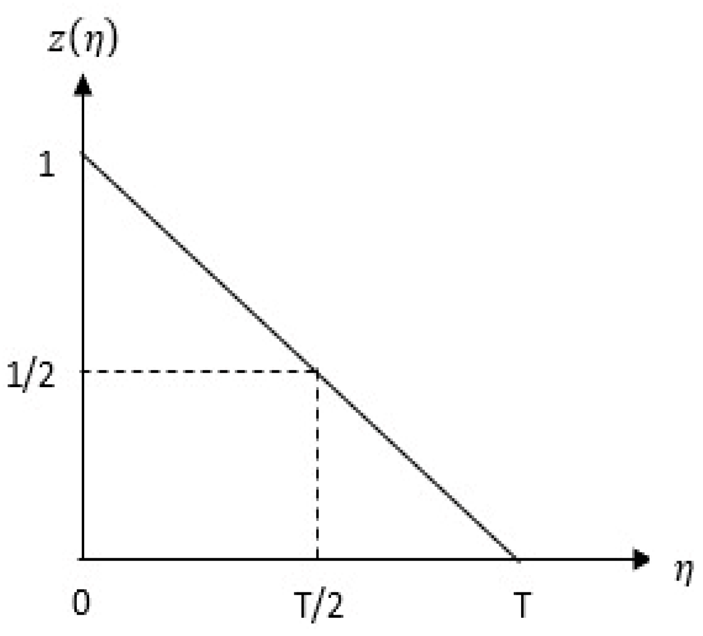
The graph above depicts how the variable z will be linked to the stress factor $\eta$. The range of variation of the stress factor is chosen as $0\le \eta \le T.$ When the stress factor reaches its maximum value, the system will fail. Here, the geometric model is as follows,

$$p_s=zp.$$

(24)

Reliability in the natural environment is denoted by p and reliability under stress by $p_s.$The association of the stress measurement value with the parameter $t\ge 0$can be undertaken in basically two different ways,

$$0\le \eta \le T \iff 0\le t<\infty or 0\le t\le EX.$$

(25)

According to the above choice, one of two different models will be preferred. Here, let us first choose $0\le t<\infty .$ Thus, we can choose the stress factor $\eta =\eta \left(t\right)$ as follows,

$$\eta =T{F}_M\left(t\right).$$

(26)

Here, $M~F_M\left(t\right)$is the distribution function of a random variable $M$. At the same time, $M$ is not related to the running time of the system.

Now let us take the equation $z=z\left(\eta \right)$ as an example, as follows,

$$z=1-\eta /T.$$

(27)

The graph of this function is in Figure 4,

In addition, let us choose the distribution function in Equation (26) as follows,

$$F_M\left(t\right)=1-\exp \left(-mt\right).$$

(28)

Thus, if the value of the stress factor $\eta$is taken into account, the mitigation variable and the reliability under stress will be, respectively, as follows,

$$z=\exp \left(-mt\right)$$

(29)

$$p_s=\exp \left(-mt\right)p.$$

(30)

When the running time of the system $Exp\left(\lambda \right)$ is chosen, $p_s=\exp \left(-\left(m+\lambda \right)t\right)$ is obtained. This result shows us that the distribution of the running time of the system operating under stress is exponential with parameter $m+\lambda$. Taking all these into account, we can calculate the following conditional probability at this point,

$$\begin{gathered} Pr\left\{X_s>t-h|X>t\right\}=Pr\left\{M>t-h|X>t\right\}Pr\left\{X>t-h|X>t\right\} \\ =Pr\left\{M>t-h|X>t\right\} : Pr\left\{X>t-h|X>t\right\}=1 \\ =Pr\left\{M>t-h\right\}=\exp \left(-m\left(t-h\right)\right) : M and X are independent \end{gathered}$$

(31)

The conditional probability calculated here is very important to emphasize the importance of the stress factor. When it is known that the runtime of the system in a normal environment is greater than $t$, a decrease of $h>0$ indicates the reliability of the system under stress.

The following table shows the reliability of the system in natural and stressed environments for $m=0.5, \lambda =0.1.$

When the system reliabilities in

Table 3. Reliabilities calculated over time.

$\mathit{p}$	${\mathit{p}}_{\mathit{s}}$	$\mathit{t}$
1.000	1.000	0.0
0.990	0.942	0.1
0.980	0.887	0.2
0.970	0.835	0.3
0.960	0.787	0.4
0.951	0.741	0.5
0.941	0.698	0.6
0.932	0.657	0.7
0.923	0.619	0.8
0.913	0.583	0.9
0.904	0.549	1.0
0.895	0.517	1.1
0.886	0.487	1.2
0.878	0.458	1.3
0.869	0.432	1.4
0.860	0.406	1.5
0.852	0.383	1.6
0.843	0.361	1.7
0.835	0.340	1.8
0.826	0.320	1.9
0.818	0.301	2.0
0.810	0.283	2.1
0.802	0.267	2.2
0.794	0.252	2.3
0.786	0.237	2.4
0.778	0.223	2.5
0.771	0.210	2.6
0.763	0.200	2.7
0.755	0.186	2.8
0.748	0.175	2.9
0.740	0.165	3.0
0.733	0.155	3.1
0.726	0.146	3.2
0.718	0.138	3.3
0.711	0.130	3.4
0.704	0.122	3.5
0.697	0.115	3.6
0.690	0.109	3.7
0.683	0.102	3.8
0.677	0.096	3.9
0.670	0.090	4.0

are considered, it can be seen that the stress factor chosen for this example reduces the reliabilities by $1/(m+\lambda )=5/3.$ In addition to this table, some conditional probability values are shown in

Table 4. Some conditional reliability values of the system under stress.

$\mathit{P}\mathit{r}\left\{{\mathit{X}}_{\mathit{s}}>\mathit{t}-\mathit{h}|\mathit{X}>\mathit{t}\right\}$	$\mathit{t}$	$\mathit{h}$	$\mathit{t}-\mathit{h}$
0.637	1	0.1	0.9
0.670		0.2	0.8
0.704		0.3	0.7
0.740		0.4	0.6
0.778		0.5	0.5
0.386	2	0.1	1.9
0.406		0.2	1.8
0.427		0.3	1.7
0.449		0.4	1.6
0.472		0.5	1.5
0.234	3	0.1	2.9
0.246		0.2	2.8
0.259		0.3	2.7
0.272		0.4	2.6
0.286		0.5	2.5
0.142	4	0.1	3.9
0.149		0.2	3.8
0.157		0.3	3.7
0.165		0.4	3.6
0.173		0.5	3.5

,

The conditional reliabilities in Table 4 are larger than the system reliabilities under stress in Table 3. The condition used here is not the observation condition. It is the reliability of a system with a given instantaneous reliability or probability of operation in the natural environment at a smaller instant than this time under stress.

In this example, the reliability of the system and the distribution chosen for stress are arbitrary, but similar examples can be increased for different distributions. The method used is different in content from some methods used in the literature. For example, in Pfanz, H. et al. [2] and Chandra, A. et al. [3], a similar problem is addressed but the methodology is different. The difference in the methods applied in our example and in these two studies in the literature is due to the data structure. While the methods of these two studies cannot be adapted to our example, the method we use in our example can be easily adapted to the data of these two literatures. In the example constructed here, the $0\le \eta \le T \iff 0\le t<\infty$ part of expression (25) was used. Similarly, the $0\le \eta \le T\iff 0\le t\le EX$ part can also be used easily.

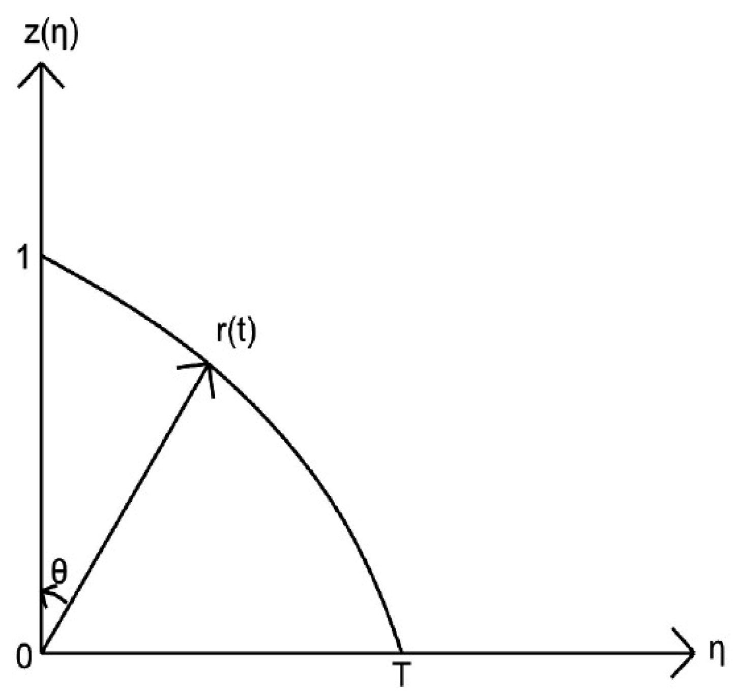
Now, in the remainder of this section, let us show that the reduction factor visualized in Figure 3 can also be configured as polar or angular. For this, consider Figure 5.

The figure above consists of a vector of length $||r\left(0\right)||=1$ to $||r\left(T\right)||=T$ and the angle that this vector makes with the component that is the stress measure. Since only two- and three-dimensional drawings are possible in geometric representations, we can only include one or two stress factors. The reliability under the stress factor is taken as in Equation (24), where $p$ is the reliability of the system and $z$ is the mitigation component.

In Figure 5, the angle $r\left(t\right)$ vector makes with z is $\theta =\pi /2$ while $t=0, z=||r\left(0\right)||=1$ and $p_s=p$. This shows us that there is no stress factor at the beginning. As the angle increases from zero to $\pi /2$ the $z$ component will decrease from one to zero. This will decrease the reliability of $p_s$ from $p$ to zero. In Figure 5, the horizontal axis values are equal to rsint and the vertical axis values are equal to $rcost.$ Here it is simply represented by $||r\left(t\right)||=r$.

Again, let us represent the values of the reduction factor under two stress factors as in Figure 4. In this case, the length of the vector is as in the following equation,

$$r=\sqrt{{\eta }^2+{\left(1-{\displaystyle \frac{\eta }{T}}\right)}^2.}$$

(32)

Note that the variable $\eta$ is obtained as follows,

$$\eta ={\displaystyle \frac{tg\theta }{1+tg\theta /T}}.$$

(33)

Since the reduction factor will depend on both $r$ and$\theta$, let us define the parameter $\theta$ depending on the distribution function as follows,

$$\theta ={\displaystyle \frac{\pi }{2}}{F}_M\left(t\right).$$

(34)

Considering the above two equations, the reduction factor is obtained as follows,

$$z=cos\left({\displaystyle \frac{\pi }{2}}{F}_M\left(t\right)\right)\sqrt{{\eta }^2+{\left(1-{\displaystyle \frac{\eta }{T}}\right)}^2}.$$

(35)

Here, again, $F_M$ is the distribution function of a $M$ random variable. Now let us calculate Table 3 values under this assumption.

The reliabilities under stress calculated in

Table 5. T = 10 is taken in calculations.

$\mathit{p}$	${\mathit{p}}_{\mathit{s}}$	$\mathit{z}$	$\mathit{\theta }$	$\mathit{r}$	$\mathit{\eta }$	$\mathit{t}$
1.000	1.000	1	0	1		0.0
0.990	0.982	0.992	0.076	0.995	0.075	0.1
0.980	0.965	0.984	0.149	0.996	0.147	0.2
0.970	0.947	0.977	0.218	1.001	0.216	0.3
0.960	0.932	0.971	0.284	1.012	0.283	0.4
0.951	0.917	0.965	0.347	1.026	0.349	0.5
0.941	0.902	0.958	0.407	1.043	0.413	0.6
0.932	0.887	0.952	0.463	1.064	0.476	0.7
0.923	0.873	0.946	0.517	1.088	0.539	0.8
0.913	0.858	0.940	0.569	1.115	0.601	0.9
0.904	0.844	0.933	0.618	1.145	0.663	1.0
0.895	0.830	0.927	0.664	1.178	0.726	1.1
0.886	0.816	0.921	0.708	1.213	0.789	1.2
0.878	0.803	0.914	0.750	1.250	0.853	1.3
0.869	0.789	0.908	0.790	1.291	0.917	1.4
0.860	0.775	0.902	0.828	1.334	0.983	1.5
0.852	0.762	0.895	0.864	1.379	1.050	1.6
0.843	0.749	0.888	0.899	1.427	1.117	1.7
0.835	0.736	0.881	0.932	1.478	1.187	1.8
0.826	0.722	0.874	0.963	1.531	1.257	1.9
0.818	0.709	0.867	0.992	1.587	1.329	2.0
0.810	0.696	0.860	1.021	1.645	1.403	2.1
0.802	0.684	0.852	1.047	1.706	1.478	2.2
0.794	0.671	0.845	1.073	1.769	1.555	2.3
0.786	0.658	0.837	1.097	1.835	1.634	2.4
0.778	0.645	0.829	1.120	1.904	1.714	2.5
0.771	0.633	0.821	1.142	1.975	1.797	2.6
0.763	0.620	0.812	1.163	2.049	1.882	2.7
0.755	0.607	0.804	1.183	2.126	1.968	2.8
0.748	0.595	0.795	1.202	2.205	2.057	2.9
0.740	0.582	0.786	1.220	2.286	2.147	3.0
0.733	0.569	0.777	1.237	2.371	2.240	3.1
0.726	0.557	0.767	1.253	2.457	2.335	3.2
0.718	0.544	0.758	1.269	2.547	2.432	3.3
0.711	0.532	0.748	1.283	2.638	2.530	3.4
0.704	0.519	0.738	1.297	2.733	2.631	3.5
0.697	0.507	0.728	1.311	2.829	2.734	3.6
0.690	0.495	0.717	1.323	2.928	2.839	3.7
0.683	0.483	0.707	1.335	3.029	2.946	3.8
0.677	0.471	0.696	1.347	3.133	3.055	3.9
0.670	0.459	0.685	1.358	3.239	3.166	4.0

are higher than those in Table 3. However, the scenarios assumed for both tables are similar and the parameters of the exponential distributions are the same. Nevertheless, the reason for this difference is that the mitigation factor used in Table 5 has a different story. This clearly shows the importance of diversity in the methods used.

6. Fourth Critical Approach: Differential Interpretation of the Stress Factor

The parameters of operating systems are naturally estimated by simulations of continuous variables. For this reason, the interpretation of the stress factor by examining its differential properties as well as its geometric interpretation can provide some details in the analysis. The concept of differential in its general form defines the trajectory of a curve or a surface in a certain direction. This trajectory is briefly analyzed depending on the function increment. Therefore, the differential is defined as the linear head of the function increment. Of course, there are many detailed definitions in mathematical sources. However, when interpreted, all of them are equivalent to our short definition. Since differential equations contain more general classes of functions, they are more helpful in describing phenomena. In this respect, it is easy to construct a first derivative differential equation by taking the derivatives of both sides of the relation given by (24) and considering the following relation, which is valid for some reliabilities. The relationship valid for some reliabilities is as follows,

$$p^{\prime }=gp.$$

(36)

Here, g is a constant factor independent of the variable in which the derivative is taken. For example,

$$F\left(t\right)=1-exp\left(-\lambda t\right) \Rightarrow p\left(t\right)=exp\left(-\lambda t\right) \Rightarrow p^{\prime }=\lambda exp\left(-\lambda t\right) \Rightarrow g=-\lambda$$

Now, let us note the following steps with $p_s=up$,

$${p_s}^{\prime }=u^{\prime }p+ugp : p^{\prime }=gp$$

$${p_s}^{\prime }=u^{\prime }p+g{p}_s : p_s=up$$

$${p_s}^{\prime }-g{p}_s=u^{\prime }p.$$

(37)

In the last step, a linear differential equation is obtained. While obtaining this equation, it should not be ignored that $p^{\prime }=gp$ for reliability. The solution of the differential equation given by (37) easily gives us the reliability of the system operating under stress. However, when we want to choose a special one among the family of solutions, we need to determine the special conditions of the system and use it. The solution of the differential equation given by (37) will be as follows,

$$p_s=exp\left\{\int gdt\right\}\left\{\int exp\left\{\int -gdt\right\}{u}^{\prime }pdt+K\right\}$$

$$p_s=exp\left\{gt\right\}\left\{\int exp\left\{-gt\right\}{u}^{\prime }pdt+K\right\}.$$

(38)

Similarly, a different version of Equation (37) can be obtained,

$$p{u}^{ˊ}+gpu={p_s}^{\prime }$$

$$u^{\prime }+gu={p_s}^{\prime }/p.$$

(39)

The solution of this equation is as follows,

$$u=exp\left\{-gt\right\}\left\{\int exp\left\{gt\right\}\left({p_s}^{\prime }/p\right)dt+K\right\}.$$

(40)

Naturally, this solution gives us the expression of the reduction factor. It is appropriate to use whichever equation the information obtained for the system allows us to solve. Since the integral cannot be taken analytically in both (38) and (40), numerical solutions should be used. In (38), when p is known, numerical values of the reduction factor should be observed instead of its analytical expression, and in (40), when p is known, numerical values of the reliability under stress should be observed. Numerical solutions of Equation (40) can be obtained using the values of Table 3 as an example. In

Table 6. Some numerical values for$u.$

$\mathit{p}$	${\mathit{p}}_{\mathit{s}}$	${{\mathit{p}}_{\mathit{s}}}^{\prime }$	${{\mathit{p}}_{\mathit{s}}}^{\prime }/\mathit{p}$	$\mathit{u} \left(Prediction\right)$	$\mathit{u} \left(Real\right)$	$\mathit{t}$
1.000	1.000					0.0
0.990	0.942	−0.58	−0.58	0.9318	0.95	0.1
0.980	0.887	−0.55	−0.56	0.8691	0.91	0.2
0.970	0.835	−0.52	−0.53	0.8120	0.86	0.3
0.960	0.787	−0.48	−0.50	0.7647	0.82	0.4
0.951	0.741	−0.46	−0.48	0.7157	0.78	0.5
0.941	0.698	−0.43	−0.46	0.6739	0.74	0.6
0.932	0.657	−0.41	−0.44	0.6349	0.70	0.7
0.923	0.619	−0.38	−0.41	0.6079	0.67	0.8
0.913	0.583	−0.36	−0.39	0.5783	0.64	0.9
0.904	0.549	−0.34	−0.38	0.5432	0.61	1.0
0.895	0.517	−0.32	−0.36	0.5208	0.58	1.1
0.886	0.487	−0.30	−0.34	0.5024	0.55	1.2
0.878	0.458	−0.29	−0.33	0.4758	0.52	1.3
0.869	0.432	−0.26	−0.30	0.4774	0.50	1.4
0.860	0.406	−0.26	−0.30	0.4428	0.47	1.5
0.852	0.383	−0.23	−0.27	0.4529	0.45	1.6
0.843	0.361	−0.22	−0.26	0.4372	0.43	1.7
0.835	0.340	−0.21	−0.25	0.4234	0.41	1.8
0.826	0.320	−0.20	−0.24	0.4117	0.39	1.9
0.818	0.301	−0.19	−0.23	0.4018	0.37	2.0
0.810	0.283	−0.18	−0.22	0.3939	0.35	2.1
0.802	0.267	−0.16	−0.20	0.4076	0.33	2.2
0.794	0.252	−0.15	−0.19	0.4041	0.32	2.3
0.786	0.237	−0.15	−0.19	0.3812	0.30	2.4
0.778	0.223	−0.14	−0.18	0.3806	0.29	2.5
0.771	0.210	−0.13	−0.17	0.3818	0.27	2.6
0.763	0.200	−0.10	−0.13	0.4558	0.26	2.7
0.755	0.186	−0.14	−0.19	0.2918	0.25	2.8
0.748	0.175	−0.11	−0.15	0.3707	0.23	2.9
0.740	0.165	−0.10	−0.14	0.3780	0.22	3.0
0.733	0.155	−0.10	−0.14	0.3603	0.21	3.1
0.726	0.146	−0.09	−0.12	0.3975	0.20	3.2
0.718	0.138	−0.08	−0.11	0.4097	0.19	3.3
0.711	0.130	−0.08	−0.11	0.3947	0.18	3.4
0.704	0.122	−0.08	−0.11	0.3798	0.17	3.5
0.697	0.115	−0.07	−0.10	0.3954	0.16	3.6
0.690	0.109	−0.06	−0.09	0.4124	0.16	3.7
0.683	0.102	−0.07	−0.10	0.3677	0.15	3.8
0.677	0.096	−0.06	−0.09	0.3864	0.14	3.9
0.670	0.090	−0.06	−0.09	0.3736	0.13	4.0

shows the calculation of numerical values of the reduction factor for some values of $t>0 K=1.$

7. Discussion

System analysis is basically an important application area of stochastic processes. System reliability is a direct probabilistic expression and is a frequently used parameter in system analysis. Probabilistic expressions can be empirically selected from possible outcomes or they can be based on mass properties. A usage error in probability that we do not pay much attention to is the old saying, ‘What is the probability of getting heads when a coin is tossed in the air and lands on the ground?’ or ‘What is the probability of getting tails when a coin is tossed in the air and lands on the ground? ‘What is the probability of getting heads when it falls?’ Which of the two questions can be related to probability? Of course, it is the second one, because the first one is an event that has already happened, and it makes more sense to look at the money falling on the ground instead of talking about its probability. This short story actually tells us the difference between ‘observation’ and ‘hypothesized’ situations. The paradox used for ordinal statistics in the first part of our study actually belongs to this. A working technical system changes structure at the moment of observation. For example, an F system with 5 outputs out of 10 has now turned into an F system with 3 outputs out of 8 from the moment the second component is disturbed. However, since the system reliability is inherently calculated before the system starts operating, this is ignored. Many examples can be found in the literature, e.g., Eryılmaz, S. [5,14,15], for the study of systems with $\mathrm{n}\mathrm{to}\mathrm{k}$ outputs on purely hypothetical cases.

In the second part of the findings, the focus is more on how to define the effects of the stresses affecting the system on the average runtime and geometric and differential interpretations of the stress are given. At the beginning of this part, the mean running time is conceived as the load on the distribution function of a specially defined vector field. Factors that decrease the load are structures that shift the vector field to the left, and factors that increase the load are structures that shift the vector field to the right. The natural environment is a vector field with no horizontal component. This is also a very important definition. The width of the distribution function on the vertical axis is only one unit. In this case, there is no chance that the average runtime in the natural environment is infinite. Because the load on the distribution function of a vector field without horizontal component in the region without slope is zero. Over the whole range of definitions$, \overrightarrow{E}X$ is the average running time under stress. However, it is not easy to measure the effect of stress on the average working time at any given moment. In particular, average working time is not a value calculated at a given moment. However, if we want to calculate the average in a restricted sub-interval instead of the whole range, it is possible to calculate it with the help of a conditional distribution. For example, the exponential distribution with parameter $\lambda =0,1$used in Table 3 has a mean $EX=10$ over the whole range of definition, but some conditional means of both systems are calculated in the table below.

In

Table 7. Conditional averages calculated over a duration in normal and stress conditions.

$\mathit{p}$	$\mathit{f}$	$\mathit{E}\left\{\mathit{X}|\mathit{X}<\mathit{a}\right\}$	${\mathit{p}}_{\mathit{s}}$	${\mathit{f}}_{\mathit{s}}$	$\overrightarrow{\mathit{E}}\left\{\mathit{X}|\mathit{X}<\mathit{a}\right\}$	$\mathit{t}$
1.000	0		1.000	0		0.0
0.990	0.01		0.942	0.058		0.1
0.980	0.01		0.887	0.055		0.2
0.970	0.01		0.835	0.052		0.3
0.960	0.01		0.787	0.048		0.4
0.951	0.009		0.741	0.046		0.5
0.941	0.01		0.698	0.043		0.6
0.932	0.009		0.657	0.041		0.7
0.923	0.009		0.619	0.038		0.8
0.913	0.01		0.583	0.036		0.9
0.904	0.009	0.542	0.549	0.034	0.500	1.0
0.895	0.009		0.517	0.032		1.1
0.886	0.009		0.487	0.030		1.2
0.878	0.008		0.458	0.029		1.3
0.869	0.009		0.432	0.026		1.4
0.860	0.009		0.406	0.026		1.5
0.852	0.008		0.383	0.023		1.6
0.843	0.009		0.361	0.022		1.7
0.835	0.008		0.340	0.021		1.8
0.826	0.009		0.320	0.020		1.9
0.818	0.008	1.015	0.301	0.019	0.856	2.0
0.810	0.008		0.283	0.018		2.1
0.802	0.008		0.267	0.016		2.2
0.794	0.008		0.252	0.015		2.3
0.786	0.008		0.237	0.015		2.4
0.778	0.008		0.223	0.014		2.5
0.771	0.007		0.210	0.013		2.6
0.763	0.008		0.200	0.010		2.7
0.755	0.008		0.186	0.014		2.8
0.748	0.007		0.175	0.011		2.9
0.740	0.008	1.474	0.165	0.010	1.123	3.0
0.733	0.007		0.155	0.010		3.1
0.726	0.007		0.146	0.009		3.2
0.718	0.008		0.138	0.008		3.3
0.711	0.007		0.130	0.008		3.4
0.704	0.007		0.122	0.008		3.5
0.697	0.007		0.115	0.007		3.6
0.690	0.007		0.109	0.006		3.7
0.683	0.007		0.102	0.007		3.8
0.677	0.006		0.096	0.006		3.9
0.670	0.007	1.913	0.090	0.006	1.557	4.0

, conditional means are calculated with the distribution values from Table 3. Note that the means under stress are lower than the other means. The differences are the calculated values of the function from Equation (20).

$$g\left(s\right)={{\displaystyle \int }}_0^{s}y\left(t\right)dt.$$

Thus, $g\left(0\right)=0, g\left(1\right)=0.042$, $g\left(2\right)=0.201$, $g\left(3\right)=0.552$, $g\left(4\right)=0.908$ are easily obtained. Note that these values belong to a function basically deformed from $x/\left(1+x\right)$ which takes values in the range of zero and one. Therefore, the regression estimation of the function $g\left(s\right)$ can be performed easily. However, the calculation procedure can also work in the opposite direction.

Note that the geometric interpretation of the stress factor is based on Equation (24). Therefore, depending on the parameter, the variable z used as a reduction factor changes from one to zero. As an example, a simple linear decreasing structure is used in the relevant section.

Let us consider the following data as an example. In the data, $\lambda =0.01$ is taken.

In

Table 8. Model parameters calculated from the observed stress value over time.

$\mathit{t}$	$\mathit{\eta }$	$\mathit{p}$	${\mathit{p}}_{\mathit{s}}$	$\mathit{z}$	$\mathit{r}$	$\mathit{\theta }$
0–5	2	0.95	0.87	0.92	2.2	65.29
5–10	2.2	0.9	0.74	0.83	2.35	69.33
10–15	2.5	0.86	0.62	0.72	2.6	73.93
15–20	2.7	0.82	0.57	0.7	2.78	75.46
20–25	2.8	0.78	0.5	0.65	2.87	76.93
25–30	3	0.74	0.47	0.64	3.06	77.95
30–35	3.4	0.7	0.4	0.58	3.45	80.32
35–40	4.5	0.67	0.38	0.57	4.53	82.78
40–45	5	0.64	0.33	0.52	5.02	84.06
45–50	6	0.6	0.27	0.45	6.02	85.71
50–55	9	0.58	0.23	0.4	9	87.45
55–60	12	0.55	0.2	0.38	12	88.18

, the stress factor, $\eta$, is designed for increasing values and observed over time. Since the operating performance of the system is known in a normal environment, reliability values can be calculated. However, ps values must also be observed in the experiment. For this, the scenario should be designed according to the number of systems operating at $\eta$ stress value at the end of t time interval. Of course, this brings along an important data source. Therefore, it is always more beneficial to design the scenario in the opposite direction. This means knowing the mass distributions.

The stochastic analysis of running systems, or in general terms, living systems, is a type of analysis that is used by many disciplines. In general, research based on physical foundations is in the field of engineering, and research based on biological foundations is in both engineering and medicine, such as genetic engineering. Much of this work is in areas related to the growth or shrinkage of living systems. For example, Khain, E. et al. [16] investigated special types of differential equations and their solutions developed for biological research. Differential equation structures developed for biological research often operate on a class of curve types that tend to grow or shrink. The most basic example of this is the logistic model. Of course, as research has developed, equation families have increased and different solution methods have been sought. Ilatı, M. [17] and Corti, M. et al. [18] are just two of the many examples in the literature. While the first of these works used the Galerkin method for the Kolmogorov equation, the second one investigated the use of the discontinuous Galerkin method. For Markov chains with continuous time and continuous state space, the Kolmogorov differential equation is a very important structure. Of course, since this equation covers a general class, its family of solutions is capable of encompassing many researches. In the ’differential interpretation of stress’ part of our work, two inhomogeneous linear differential equations with constant coefficients are considered. The solutions of these equations are found in Equations (38) and (40). In this respect, methods such as Galerkin’s method were not used for the solution. However, numerical calculations are still valid for these equations. Of course, the given differential equations are in the class of functions $p^{\prime }=gp$. It should be noted that Equations (38) and (40) present successive solutions of each other. This presents us with a sequential computation process. However, we generally prefer to operate under the assumption that the mass distribution of stress is known within the reliability calculation, for example, Gökdere, G. et al. [9], Bhattacharyya, G. K. et al. [19].

Let us immediately note below an important feature that should not be overlooked in the differential interpretation of stress.

$$t_0=max\left\{t : u\left(t\right)=1\right\}$$

$$p_s\left(t_0+h\right)=u\left(h\right)p\left(t\right)$$

$$p_s\left(t\right)=p\left(t\right), t\le t_0$$

$${\displaystyle \frac{p_s\left(t_0+h\right)-p_s\left(t_0\right)}{h}}={\displaystyle \frac{u\left(h\right)-1}{h}}p\left(t_0\right)$$

$${p^{\prime }}_s\left(t_0\right)=u^{\prime }\left(0\right)p\left(t_0\right).$$

This property is almost never taken into account in most geometric processes. For example, Brown, KS et al. [20] and similar works can be found in the literature. The mathematical models used in such studies involving a decreasing factor cannot take this property into account since they try to represent the decreasing factor in an analytical expression. In models involving differential equations, this feature cannot be emphasized since the differential is not defined at the break points. Therefore, the decay is analyzed after the process starts. Nevertheless, the same problem applies to Equations (38) and (40). However, since our solutions are in the class of functions that satisfy the above property, they can be analyzed in the mathematical model.

8. Conclusions

Understanding the structure of a working system is a very difficult process, even though it may seem simple at first glance. By ‘seemingly simple’, we mean that a working system should be evaluated only in terms of its structural characteristics at first glance. However, a working system should be evaluated together with its working environment and we should not forget that the working process is related to more than one factor. The most important assumption that we want to emphasize from the very beginning in this study is the idea that a system operated in an ideal environment can work forever. However, the environments in which systems with an average runtime operate have factors that prevent the system from working. As a simple example, an object thrown in an environment without gravity and friction should travel at the same speed forever in the direction it was thrown. On the other hand, an object thrown in the world, that is, in an environment with gravity and friction, shows an oblique throw shape, as it is called in physics, and after a while it succumbs to gravity and its movement ends. Therefore, systems designed in natural working environments succumb to the stress caused by their natural environment after a while and complete their working period. In short, we call the stress in their natural environment natural stress. When other stresses are added on top of this assumed natural stress, the system uptime drops below the designed average. It is possible to find an indefinite number of studies in the literature. As we mentioned in the related paragraphs, we had the opportunity to mention a small number of them in this study: Mazzanti, G. [1], Pfanz, H., Vollrath et al. [2], Chandra, A. et al. [3].

An arbitrary component of a multi-component system that fails does not necessarily fail the system. At first glance, there seems to be no correlation between the moment of failure and the moment of failure of the system, but this is closely related to the distribution functions of the uptime of the components. For example, in a parallel connected system, when the component with the largest average runtime fails, the system should fail, but we have to calculate the reliability of the system from the distribution of the maximum sequence statistic. This is because the runtime distributions start from $t>0$. In the production of the component with the largest average uptime, there may be products whose uptime is much lower than the average. Therefore, sequence statistics form the basis of reliability theory. Therefore, the first part of the findings includes the calculation of the sequence statistics when the moment of deterioration is known. The related Equation (4) is important for us. The distribution function assumed in this equation actually describes a random variable under the condition $c_{k-1}<t<c_k$, i.e., between two consecutive deterioration moments when the next deterioration has not occurred, given by

$$M~U\left(0,F_k\left(c_k-c_{k-1}\right)\right).$$

This finding allows us to uncover a very important auxiliary factor describing the operating system. In particular, in Tony Ng et al. [9] and Eryilmaz, S. [5], the lack of such a factor of $M$ variable is felt even though it was not used in these two studies. Why? It is not a correct assumption to assume that the time between successive failure moments of a system whose runtimes are exponential, or even to assume that the order-dependent failure moments in the system are exponential. Instead, it is more accurate to use the memorylessness property of the system, which can now be taken exponential when any moment of deterioration is known. The system is defined separately by the times between consecutive deterioration moments.

The values in Table 3 of Section 5 show the reliability of a technical system in natural and stressful environments depending on the selected parameters. The values in Table 7 were calculated based on this table. The two calculations we will pay attention to in Table 7 are the conditional averages $E\left\{X|X<a\right\}, \overrightarrow{E}\left\{X|X<a\right\}$. If we pay attention to Table 7, it is seen that the $E\left\{X|X<a\right\}$ averages are greater than the $\overrightarrow{E}\left\{X|X<a\right\}$ values. The reason for this is that the stress factor is taken into account when calculating the $\overrightarrow{E}\left\{X|X<a\right\}$ averages.

Basically, in the geometric interpretation, the shapes are chosen to be planar. But it can also be moved into three dimensions. Figure 6 illustrates this easily.

Here the axis values are parametrically as follows.

$$z=rcos\theta$$

$$l=rsin\theta$$

$$\eta =rsin\theta cos\Phi$$

$$\xi =rsin\theta sin\Phi$$

In the section on the differential interpretation of the stress factor, two solutions given by Equations (38) and (40) are proposed. The one in (38) gives the reliability values under stress. In order to calculate this integral, the first priority is to know the reduction factor analytically. If this is not possible, an approximate calculation can also give us an approximate solution. Observation values need to have smaller time intervals. However, if the mass distribution of this factor is known, this will simplify the procedure. The same is true for Equation (40).

• Recommendations

Examining the correlation between the variables defined for the geometric structure of the stress factor in this study is left to future studies. The numerical values considered in the study are designed based on a single factor. However, the types of stress present in the environment may be more than one. In this case, it is appropriate to use three components for stress. Spherical coordinates can be used in this study. In addition, it is important to consider the stress present in the environment when calculating the average life span of the system. For this, the expected value operator completed in the vector field can be used. While discussing the geometric structure of the stress factor, planar or three-dimensional stress factors are naturally considered. This situation necessitates us to consider some restrictions. If we want to create a wider analysis area, it is quite useful to design the stress structure as a vector field.