Abstract
This article is dedicated to the construction of neural networks for the prediction of the current–voltage characteristic (CVC). CVC is the most important characteristic of the mass transfer process in electro-membrane systems (EMS). CVC is used to evaluate and select the optimal design and effective operating modes of EMS. Each calculation of the CVC at the given values of the input parameters, using developed analytical-numerical models, takes a lot of time, so the CVC is calculated in a limited range of parameter changes. The creation of neural networks allowed for the use of prediction to obtain the CVC for a wider range of input parameter values and much faster, saving computing resources. The regularities of the behavior of CVC for various values of input parameters were revealed. During this work, several different neural network architectures were developed and tested. The best predictive results on test samples are given by the neural network consisting of convolutional and LSTM (Long Short-Term Memory) layers.
1. Introduction
Electro-membrane systems (EMS) are advanced technological platforms widely employed in numerous industrial applications, including purification, separation, enrichment, desalination, and concentration of liquid and gas mixtures. These systems have proven indispensable in fields such as chemical and petrochemical industries, food technology, biotechnology, and pharmaceuticals. A critical parameter for understanding and optimizing the performance of EMS is the current–voltage characteristic (CVC), which serves as an integral characteristic of the salt ion transport process within the desalination channel of electrodialysis devices. By analyzing the CVC, engineers and researchers can evaluate the efficiency of EMS, identify optimal design parameters, and determine effective operating regimes.
CVC encapsulates the interplay of various physical and electrochemical processes that occur during the operation of EMS. These include ion transport, fluid dynamics, and electrochemical reactions, among others. The mathematical modeling of these processes has traditionally relied on boundary-value problems related to the Nernst–Planck and Poisson (NPP) electrodiffusion equations [1,2,3,4,5,6]. These equations describe ion transport under the influence of electric fields and concentration gradients, and their coupling with the Navier–Stokes equations enables the modeling of electroconvection—the interaction between electric fields and fluid motion. Electroconvection plays a key role in enhancing ion transport, particularly under overlimiting current conditions, where the transport rate exceeds the diffusion-limited rate.
Theoretical advances in the study of electroconvection have provided critical insights into such phenomena as nonequilibrium electroosmotic slip at solution–membrane interfaces and electrochemical instability [7]. Notable contributions include the works of Zaltzman [5,7], M. Bazant, A. Mani, and others [8,9], who developed the theory of electroosmosis of the second kind and introduced detailed two-dimensional mathematical models of ion transport in EMS [10,11]. These models account for forced convection and electroconvection in the absence of chemical reactions and have facilitated the calculation of CVC under various conditions. The first numerical results for CVC demonstrated qualitative agreement with experimental data, highlighting the potential of mathematical models to describe the complex dynamics of EMS [10].
Nevertheless, significant challenges remain in the development of the theoretical and computational modeling of CVC. The processes governing ion transport in EMS are inherently nonlinear and involve coupled interactions between electric fields, ionic species, and fluid flows. Furthermore, these processes are often accompanied by secondary effects such as water dissociation, thermal convection, and concentration polarization. Experimental studies of CVC have revealed nonstationary and unstable behavior, as evidenced by fluctuations analyzed using Fourier and wavelet techniques [12,13,14,15,16]. However, the absence of adequate mathematical models limits the ability to interpret experimental data and gain a comprehensive understanding of the underlying phenomena [17,18].
A critical unresolved problem in the field is the lack of a unified approach for linking the observed patterns of CVC with the governing physical and chemical processes. This includes the classification of numerically and experimentally obtained CVCs based on input parameters such as ion concentration, applied voltage, and membrane properties. Addressing this issue is not only of fundamental scientific interest but also of practical importance, as it would enable more precise control over EMS operations in industrial applications.
In recent years, artificial intelligence (AI) has emerged as a transformative tool for addressing complex, multivariate problems in science and engineering. In the field of electrochemistry, AI techniques, particularly artificial neural networks (ANNs), have been successfully applied to model and optimize membrane separation processes [19], control desalination systems [20], and predict CVCs for various electrochemical systems. For instance, neural network-based models have been used to optimize the efficiency of reverse osmosis plants [21], simulate the behavior of membrane distillation units [22,23], and predict the performance of Schottky diodes [24,25]. These applications demonstrate the potential of AI to overcome the computational limitations of traditional modeling approaches, which often require solving complex systems of partial differential equations [26].
The computation of CVC using conventional mathematical models involves solving the coupled Nernst–Planck, Poisson, and Navier–Stokes equations over a range of spatial and temporal domains [27,28]. This process is computationally intensive, requiring significant time and resources, and is typically limited to a narrow range of input parameters. As a result, critical aspects of the mass transfer process may be overlooked, leading to incomplete or suboptimal system designs. Moreover, existing numerical algorithms for calculating CVC often face challenges in maintaining accuracy and stability, particularly in the presence of random errors or variations in input data.
To address these challenges, the goal of this study is to develop artificial neural network (ANN) models capable of accurately predicting CVC across a wide range of input parameters. By leveraging AI, this approach aims to significantly expand the dataset for which CVC can be computed, enabling a deeper understanding of the underlying processes and more effective optimization of EMS. The training and validation datasets for the ANN models are generated using a robust numerical algorithm that solves the coupled NPP and Navier–Stokes equations. This algorithm ensures high accuracy in capturing the complex dynamics of ion transport and electroconvection, providing a reliable foundation for ANN training.
Furthermore, this study seeks to bridge the gap between theoretical modeling and practical application by integrating AI-driven predictions with advanced numerical techniques. By doing so, it aims to provide a comprehensive framework for studying and optimizing EMS, addressing both the computational challenges of traditional methods and the limitations of experimental approaches. Ultimately, this work contributes to the advancement of membrane-based separation technologies, offering new insights into the design and operation of EMS for a wide range of industrial applications.
2. Materials and Methods
2.1. Two-Dimensional Model Based on the Use of the Gauss Theorem
Let us consider a two-dimensional mathematical model of non-stationary electrolyte transfer 1:1 (Figure 1) in the potentiodynamic mode (1)–(7), which we used to calculate the current–voltage characteristic [10,27].
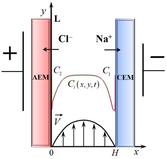
Figure 1.
Scheme of the desalination channel formed by anion-exchange (AEM) and cation-exchange (CEM) membranes of width H and length L.
The Nernst–Planck Equation (1) describes the flux of dissolved components (sodium and chlorine ions ) due to migration in an electric field, diffusion and convection, where the charge numbers of cations and anions [10]; (2) is the equation of material balance; (3) is the Poisson equation for the potential of the electric field; (4) is the equation of current flow, which means that the current flowing through the diffusion layer is determined by the flow of ions. is the dielectric constant of the solution; is the Faraday number; is the universal gas constant; T is the absolute temperature; is the potential, is the concentration; is the flux density of i-type ions; is the diffusion coefficient of the i-th ion; is the current density determined by the ion flux; is the solution flow rate; is the solution density; is the kinematic viscosity; is the pressure. The Navier–Stokes Equation (5) and continuity equations for an incompressible fluid (6) describe a velocity field formed, in particular, under the action of a forced flow and a spatial electric force. is an electric force, where the is the space charge distribution density, and is the electric field strength.
Formula (7) can be written in another way, using the Poisson Equation (3): . If we substitute (1) into (2), then Equation (2) will be written in the form
In the system of Equations (1)–(7), the quantities are unknown functions of the spatial coordinates x, y, and time .
To solve the system of Equations (1)–(7), it is necessary to specify the boundary conditions, which are determined by the area of this study, the electric field regime, the properties of the membranes, etc. [10,27].
Based on the analysis of the numerical solution of the boundary value problem of the model (1)–(7) and the boundary conditions, the main patterns of salt ion transfer are determined, and (4) is found, and the CVC is calculated.
The deriving of the stable against random errors formula for calculating the current–voltage characteristic [27] was based on the Gauss theorem [29]. For solenoidal current density , the double integral (8) has the meaning of the averaged current density:
2.2. Properties of the Current–Voltage Characteristic
Figure 2 shows a typical CVC graph—the relationship between current density and voltage. The output current was normalized to the Leveque current [30]. Along the abscissa axis is the voltage in volts.
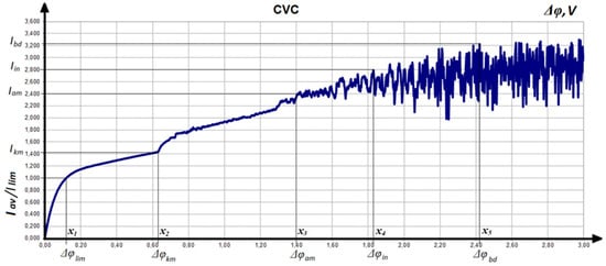
Figure 2.
Typical behavior of CVC in EMS.
We will analyze the typical behavior of CVC. The first section of the graph, when the voltage varies from 0 to , corresponds to an increase in normalized current from 0 to 1. The limit state has been reached. Between the points and current–voltage characteristic behaves like a linear function. At the point , the behavior of CVC is changing. This is caused by the beginning of electroconvection on the CEM [31]. When the voltage is increased to the value , the electroconvection begins at the AEM. The point corresponds to the interaction of electroconvective processes on CEM and AEM. The graph of CVC looks chaotic. The part of the graph between points and is characterized by the emergence of dissociation and recombination of water molecules [30]. Therefore, we no longer observe linear growth of CVC. Under the influence of increasing voltage, water molecules are divided into OH– and H+ ions (dissociation), and then these are combined again (recombination). Instead of desalination, the energy of the system is spent on these undesirable processes.
Another destructive phenomenon is space charge breakdown [31]. Its appearance corresponds to the point . Breakdown is a phenomenon that is similar to the shooting of a charge from one membrane to another. This process also prevents the growth of desalination.
2.3. Building Neural Networks Based on Calculated CVC and Analysis of Its Behavior
The main idea of modeling the current–voltage characteristics was to represent their graphs as a time series since it was important to take into account the change in current over time. In this work, we have developed an original neural network consisting of convolutional and recurrent layers to achieve a more accurate prediction of the current–voltage characteristics.
In the first stage, the CVCs were calculated for different parameters of the system (1)–(7) according to the Formula (8). For the numerical calculation, the Comsol Multiphysics package was used [32]. Figure 3 shows the interface of the developed program. The parameters of Equations (1)–(7) are supplied to the input: the initial concentration of the solution, the rate of supply of the solution to the channel, the length and width of the desalination channel, the potential jump (sweep rate), the diffusion coefficients of cations and anions, transfer numbers, etc. Information about the spacers (shape and number) was taken into account [33]. During the calculations, the processes of dissociation and recombination of water molecules were also modeled.
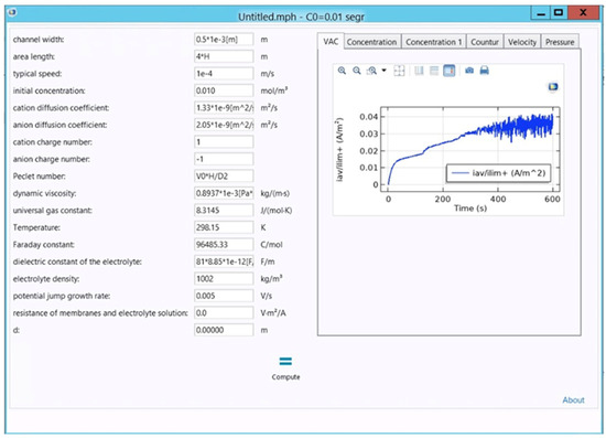
Figure 3.
The interface of the developed program for calculating CVC using Comsol Multiphysics package.
For the construction of ANN, training, control, and test data were created, which reflect the information about the relationship between input parameters of the EMS and the resulting CVC. The Adam teacher method was used to teach ANN. The result of the network is the graph points predicted for the given values of the input parameters, as well as the following data points: Using the developed network, the first 42 points of the CVC were predicted, then they were submitted to the input of the recurrent network and new 42 CVC points were predicted on their basis, etc.
3. Results
3.1. The Structure of Created Neural Networks
The choice of the structure and type of neural networks was based on an analysis of the typical behavior of CVC in EMS, which was discussed in Section 2.2. LSTM (Long Short-Term Memory—a type of recurrent neural network) layers were used to display the change in phenomena occurring in EMS. They allow us to memorize the behavior of the studied function over a long period of time. The purpose of using convolutional layers was to detect local patterns and structures in the CVC curve. Convolutional layers are able to highlight features such as peaks or dips that may indicate anomalies or important characteristics. This allows the model to analyze the CVC curve more effectively and identify unusual behavior [34]. The combination of recurrent and convolutional layers led to more accurate results in predicting current–voltage characteristics.
For the software implementation of the neural network to predict the current–voltage characteristics, the Python programming language was used, as well as the NumPy, matplotlib, pandas, scikit-learn, and keras libraries.
Let us consider the architecture of the created neural network for modeling the CVC. It is presented in Figure 4. In the beginning, we used a one-dimensional convolution with 32 filters and a kernel size of 3. A filter is a weight matrix that is applied to the input data to extract certain features. The kernel is used to denote the weight matrix of the filter. After the convolution, the ReLU activation function is applied. The input layer size is determined by the value of the number of time steps and the number of features.
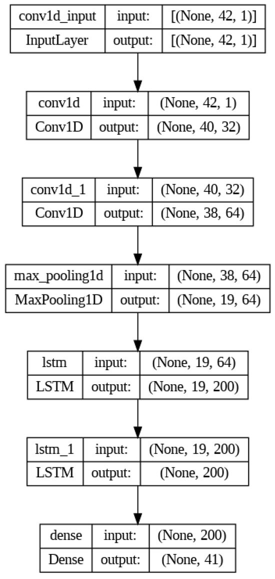
Figure 4.
The architecture of the created neural network for modeling the CVC.
Next comes a convolution layer with 64 filters and the ReLU activation function, which is also applied after the convolution. In this case, one-dimensional convolutions are used to extract local spatial features from a data sequence. Using this layer, we were able to detect dependencies between close data points. Here, one-dimensional convolution with different kernel sizes and different filters was used to extract different levels of abstraction from the input data.
Next, the output data are transferred to the two-dimensional pooling layer, which is used to reduce the dimensionality of the data by selecting the maximum feature value in each pooling window. This layer was also used to identify the most important features. In this architecture, the pooling layer helps reduce the dimensionality of the data after the convolutional layers and focuses on the most important features. Then comes the first LSTM layer with 200 units and a hyperbolic tangent activation function. Hyperbolic tangent is one of the commonly used activation functions in LSTM layers. It limits the activation values to a range between −1 and 1. Hyperbolic tangent helps the model account for long-term dependencies in sequential data and prevents gradients from growing exponentially during backpropagation. A fully connected layer is used to predict the next points in the sequence.
The architecture of the ANN includes (Figure 4):
Input layer: Accepts time series data of length 42 (current–voltage values over time).
Convolutional layers:
Layer 1: 32 filters, kernel size = 3, ReLU activation.
Layer 2: 64 filters, kernel size = 3, ReLU activation.
Pooling layer: 2D max pooling with a pooling window of size 2 × 2.
LSTM layer: 200 units, hyperbolic tangent (tanh) activation.
Fully connected (dense) layer: Outputs the predicted CVC points.
Hyperparameters:
Learning rate: 0.001 (optimized using grid search).
Batch size: 64.
Optimizer: Adam optimizer with β1 = 0.9, β2 = 0.999.
Epochs: 50.
Regularization: L2 regularization (λ = 0.01) to prevent overfitting.
Dropout: 0.3 after the LSTM layer.
The dataset consisted of 80% training, 10% validation, and 10% test data. Cross-validation was used to ensure robust performance.
3.2. Simulation of CVC Behavior by the Created Neural Network
The results of CVC modeling for two different input value sets using the created neural network are presented in Figure 5a,b. Comparison of calculated CVC (blue) with CVC received using neural network modeling (orange) at different input values (the first (a) and second (b) sets of input parameters) shows that the created neural network predicts the behavior of the CVC quite well.
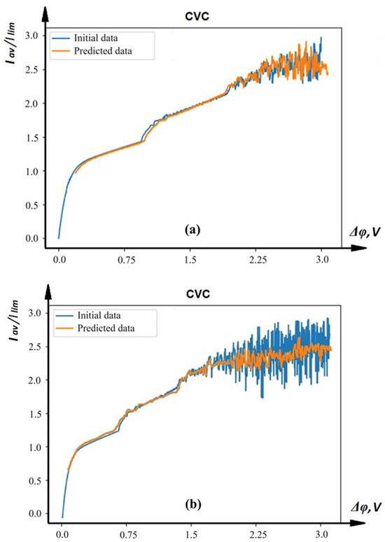
Figure 5.
Comparison of calculated CVC (blue) with CVC received using neural network modeling (orange) at different input values: the first (a) and second (b) sets of input parameters.
It can also be said that the model copes well with predicting points signaling transitions to different states of the system. The test set was prepared in advance and did not participate in training. To assess the correctness of the neural network, we used cross-validation. In the case of a limited amount of data, cross-validation is especially useful. The ANN achieved a root mean square error (RMSE) of 0.00012 and a mean absolute error (MAE) of 0.0098 on the test dataset. Comparatively, traditional numerical methods based on solving the Nernst–Planck–Poisson (NPP) equations require approximately 15–30 days for each CVC calculation, depending on the resolution of the numerical grid and hardware configuration. In contrast, the ANN model predicts the same characteristic in under 30–60 s on a standard CPU, a reduction of over 99% in computation time. Resource-wise, traditional methods demand 2–4 GB of RAM for simulations, while the ANN operates with a memory footprint of less than 500 MB.
Experimental validation was conducted using laboratory-scale EMS setups. The ANN predictions were compared to measured CVC data for two input parameter sets:
Set 1: Ion concentration = 0.1 Moll/L; channel length = 10 mm; applied voltage = 0.5–5 Volt;
Set 2: Ion concentration = 0.05 Moll/L; channel length = 8 mm; applied voltage = 0.5–4 Volt.
The experimental and ANN-predicted CVCs showed a mean absolute error (MAE) of less than 0.01 for both datasets. However, discrepancies of up to 2% were observed in overlimiting current regimes, likely due to experimental noise and unmodeled secondary effects (e.g., water dissociation).
The limitations of the proposed approach:
- The ANN model requires a large training dataset, which may not always be available for all EMS configurations, including spacers (conducting and non-conducting), their numbers, shapes, sizes, locations, dissociation and recombination of water molecules, etc.;
- It has difficulty generalizing to new input parameters (e.g., extreme ion concentrations or unusual membrane properties, structured surfaces) without additional retraining;
- The model has weak interpretability, which makes it difficult to relate the ANN output to specific physical processes.
4. Discussion
A software product for numerical calculations of CVC was created using Comsol Multiphysics. This allowed us to describe the processes occurring in the EMS desalination channel. Two-dimensional EMS models were used to create the database of CVCs. The model takes into account diffusion, migration, convective transport, electroconvection, spacers of different shapes and sizes, dissociation/recombination, and space charge breakdown. The obtained values of CVCs were used for the creation of measurement datasets (test, training, and validation).
Using a combination of convolutional and recurrent layers when implementing a neural network for CVC modeling was a good idea since they track local structures of graph behavior and also take into account the sequence. The use of convolutional layers in the architecture of neural networks allows you to track the local structure of the input data, such as peaks or dips, which indicate anomalies or unusual behavior. LSTM layers are used to model long-term dependencies such as time series. They help to take into account the context and sequence of data, as well as to store and transmit information across time steps. In the developed ANN architecture, these layers are used to model complex dependencies and obtain more accurate predictions.
It was shown that the neural network works well at different input values, which made it possible to predict current–voltage characteristics for different parameters of EMS. The values of the determination coefficient are close to 1, which also indicates a high degree of coincidence between the predicted and actual data. This suggests that the model predicts the behavior of the graph quite well on new sets of input data (not included in the training set). Also, computational efficiency guarantees the ability to quickly predict CVC.
The current ANN model is trained on data derived from a standard EMS configuration (a desalination channel with cation- and anion-exchange membranes). To generalize the model, it is possible to take the following steps:
- -
- The training dataset can be augmented with simulations of EMS configurations with different channel geometries, membrane thicknesses, and flow rates;
- -
- Transfer learning techniques can be applied to adapt the ANN to new configurations using minimal additional training data;
- -
- Preliminary tests on altered configurations (e.g., wider channels or lower ion concentrations) indicate an accuracy drop of 5–10%, highlighting the need for dataset expansion.
The ANN framework can be integrated into real-time monitoring systems for EMS by implementing the following:
- Predicting CVC in real-time based on continuously measured input parameters (e.g., voltage, ion concentration, flow rates);
- Adjusting system parameters dynamically to optimize performance (e.g., minimizing energy consumption or maximizing desalination efficiency);
- Running on edge devices or embedded systems due to its low computational requirements, enabling deployment in industrial environments with limited resources.
The proposed ANN framework could be extended to the following:
- Electrochemical systems: Predicting performance metrics for fuel cells, batteries, or electrolyzes;
- Fluid dynamics problems: Modeling flow and transport in pipelines, porous media, or microfluidic devices;
- Environmental applications: Simulating pollutant transport in water treatment systems.
These extensions could be achieved by retraining the ANN on datasets from the respective systems, leveraging its general ability to model complex physical processes.
The potential areas for future research are as follows:
- Development of hybrid models combining ANN with traditional physical models for improved generalization;
- Extension of the ANN framework to handle real-time data streams in dynamic EMS environments;
- Research on explainable AI techniques to make ANN predictions more interpretable for engineers.
The ANN model significantly reduces the time required for CVC calculations, allowing for faster design iterations of new EMS configurations and real-time monitoring of system performance in industrial environments. The application of the developed model makes it possible to save costs by minimizing the need for expensive and time-consuming experiments.
Author Contributions
Conceptualization, E.K., A.K. and M.U.; methodology, E.K.; software, A.K.; validation, E.K. and A.K.; formal analysis, E.K. and M.U.; investigation, M.U. and A.K.; resources, A.K.; data curation, E.K.; writing—original draft preparation, E.K. and M.U.; writing—review and editing, A.K.; visualization, A.K.; supervision, A.K.; project administration, E.K.; funding acquisition, E.K. and A.K. All authors have read and agreed to the published version of the manuscript.
Funding
This study was supported by the RheinMain University of Applied Sciences and the Russian Science Foundation, research project No. 24-19-00648, https://rscf.ru/project/24-19-00648/ (accessed on 22 January 2025).
Data Availability Statement
Data are contained within the article.
Conflicts of Interest
The authors declare no conflicts of interest.
References
- Newman, J.S. Electrochemical Systems; Prentice Hall: Englewood Cliffs, NJ, USA, 1973; 432p. [Google Scholar]
- McKelvey, J.P. Solid State and Semiconductor Physics; Krieger: Malabar, FL, USA, 1982; 512p. [Google Scholar]
- Lakshminarayanaiah, N. Equations of Membrane Biophysics; Academic: New York, NY, USA, 1984; 426p. [Google Scholar]
- Timashev, S.F.; Kemp, T.J. Physical Chemistry of Membrane Processes; Ellis Horwood Ltd.: London, UK, 1991; 246p. [Google Scholar]
- Rubinstein, I.; Maletzki, F. Electroconvection at an electrically inhomogeneous permselective membrane surface. Trans. Faraday Soc. 1991, 87, 2079–2087. [Google Scholar] [CrossRef]
- Kwak, R.; Pham, V.S.; Lim, K.M.; Han, J. Shear flow of an electrically charged fluid by ion concentration polarization: Scaling laws for electroconvective vortices. Phys. Rev. Lett. 2013, 110, 114501. [Google Scholar] [CrossRef]
- Rubinstein, I.; Zaltzman, B. Electro-osmotic slip and electroconvective instability. J. Fluid Mech. 2007, 579, 173–226. [Google Scholar]
- Dydek, E.V.; Zaltzman, B.; Rubinstein, I.; Deng, D.S.; Mani, A.; Bazant, M.Z. Overlimiting Current in a Microchannel. Phys. Rev. Let. 2011, 107, 118301. [Google Scholar] [CrossRef] [PubMed]
- Mani, A.; Bazant, M.Z. Deionization shocks in microstructures. Phys. Rev. 2011, E 84, 061504. [Google Scholar] [CrossRef]
- Urtenov, M.K.; Uzdenova, A.M.; Kovalenko, A.V.; Nikonenko, V.V.; Pismenskaya, N.D.; Vasil’eva, V.I.; Sistat, P.; Pourcelly, G. Basic mathematical model of overlimiting transfer enhanced by electroconvection in flow-through electrodialysis membrane cells. J. Membr. Sci. 2013, 447, 190–202. [Google Scholar] [CrossRef]
- Nikonenko, V.; Kovalenko, A.; Urtenov, M.; Pismenskaya, N.; Han, J.; Sistat, P.; Pourcelly, G. Desalination at overlimiting currents: State-of-the-art and perspectives. Desalination 2014, 342, 85–106. [Google Scholar] [CrossRef]
- Kolyubin, A.V.; Maksimychev, A.V.; Timashev, S.F. Using Flicker-noise spectroscopy to study the mechanism of the exorbitant current in a system with a cation exchange membrane. Electrochemistry 1996, 32, 227–234. [Google Scholar]
- Kolganov, V.I.; Malykhin, M.D.; Babichev, S.V.; Akberova, E.M. Analysis of the spectral composition of optical noise in a solution at the boundary with the MK-40 sulfocation exchange membrane after temperature exposure by Flicker-noise spectroscopy. Vestn. VSU Ser. Chem. Biol. Pharm. 2015, 3, 25–30. [Google Scholar]
- Budnikov, E.Y.; Kozlov, S.V.; Kolyubin, A.V.; Timashev, S.F. Analysis of fluctuation phenomena in the process of electrochemical release of hydrogen on platinum. J. Phys. Chem. 1999, 73, 530–537. [Google Scholar]
- Budnikov, E.Y.; Maksimychev, A.V.; Kolyubin, A.V.; Merkin, V.G.; Timashev, S.F. Wavelet analysis in the appendix to the study of the nature of the exorbitant current in an electrochemical system with a cation exchange membrane. J. Phys. Chem. 1999, 73, 198–213. [Google Scholar]
- Egorov, E.V.; Kozlov, V.A.; Yashkin, A.V. Phase-frequency characteristic of the transfer function of a spatially bounded electrochemical cell. Electrochemistry 2007, 43, 1–7. [Google Scholar]
- Vasil’eva, V.I.; Akberova, E.M.; Saud, A.M.; Zabolotsky, V.I. Current-Voltage Characteristics of Membranes with Different Cation-Exchanger Content in Mineral Salt—Neutral Amino Acid Solutions under Electrodialysis. Membranes 2022, 12, 1092. [Google Scholar] [CrossRef] [PubMed]
- Filingeri, A.; Gurreri, L.; Ciofalo, M.; Cipollina, A.; Tamburini, A.; Micale, G. Current distribution along electrodialysis stacks and its influence on the current-voltage curve: Behaviour from near-zero current to limiting plateau. Desalination 2023, 556, 116541. [Google Scholar] [CrossRef]
- Niemi, H.; Bulsari, A.; Palosaari, S. Simulation of membrane separation by neural networks. J. Membr. Sci. 1995, 102, 185–191. [Google Scholar] [CrossRef]
- Cabrera, P.; Cartaa, J.A.; González, J.; Melián, G. Artificial neural networks applied to manage the variable operation of a simple seawater reverse osmosis plant. Desalination 2017, 416, 140–156. [Google Scholar] [CrossRef]
- Khayet, M.; Cojocaru, C. Artificial neural network modeling and optimization of desalination by air gap membrane distillation. Sep. Purif. Technol. 2012, 86, 171–182. [Google Scholar] [CrossRef]
- Gil, J.D.; Ruiz-Aguirre, A.; Roca, L.; Zaragoza, G.; Berenguel, M. Prediction models to analyse the performance of a commercial-scale membrane distillation unit for desalting brines from RO plants. Desalination 2018, 445, 15–28. [Google Scholar] [CrossRef]
- Ismail, N.; Bouaïcha, M. Artificial Neural Network Based Prediction of the Effect of Temperature and Irradiance on Photovoltaic Current-Voltage Curves. In Proceedings of the 2022 IEEE 9th International Conference on Sciences of Electronics, Technologies of Information and Telecommunications (SETIT), Hammamet, Tunisia, 28–30 May 2022; pp. 55–60. [Google Scholar] [CrossRef]
- Güzel, T.; Çolak, A.B. Performance prediction of current-voltage characteristics of Schottky diodes at low temperatures using artificial intelligence. Microelectron. Reliab. 2023, 147, 115040. [Google Scholar] [CrossRef]
- Barkhordari, A.; Mashayekhi, H.R.; Amiri, P.; Özçelik, S.; Altındal, Ş.; Azizian-Kalandaragh, Y. Machine learning approach for predicting electrical features of Schottky structures with graphene and ZnTiO3 nanostructures doped in PVP interfacial layer. Sci. Rep. 2023, 13, 13685. [Google Scholar] [CrossRef]
- Alizadeh, S.; Bazant, M.Z.; Mani, A. Impact of network heterogeneity on electrokinetic transport in porous media. J. Colloid Interface Sci. 2019, 553, 451–464. [Google Scholar] [CrossRef] [PubMed]
- Urtenov, M.K.; Kovalenko, A.V.; Sukhinov, A.I.; Chubyr, N.O. Gudza, V.A. Model and numerical experiment for calculating the theoretical current-voltage characteristic in electro-membrane systems. IOP Conf. Ser. Mater. Sci. Eng. 2019, 680, 012030. [Google Scholar] [CrossRef]
- Kirillova, E.; Kovalenko, A. Using machine learning and artificial intelligence methods to study the current-voltage characteristics of membrane systems. In Proceedings of the 2024 World Congress on Advances in Civil, Environmental, & Materials Research (ACEM24), Seoul, Republic of Korea, 19–22 August 2024. [Google Scholar]
- Landau, L.D.; Lifshitz, E.M. Theoretical Physics. Electrodynamics of Continuous Media, 2nd ed.; Science (Nauka): Moscow, Russia, 1982; 621p. [Google Scholar]
- Uzdenova, A.M.; Kovalenko, A.V.; Urtenov, M.K.; Nikonenko, V.V. Theoretical Analysis of the Effect of Ion Concentration in Solution Bulk and at Membrane Surface on the Mass Transfer at Overlimiting Currents. Russ. J. Electrochem. 2017, 53, 1254–1265. [Google Scholar] [CrossRef]
- Kovalenko, A.; Chubyr, N.; Uzdenova, A.; Urtenov, M. Theoretical Investigation of the Phenomenon of Space Charge Breakdown in Electromembrane Systems. Membranes 2022, 12, 1047. [Google Scholar] [CrossRef] [PubMed]
- Gudza, I.V.; Kovalenko, A.V.; Urtenov, M.K.; Pismenskiy, A.V. Artificial intelligence system for the analysis of theoretical and experimental current-voltage characteristics. J. Phys. Conf. Ser. 2021, 2131, 022089. [Google Scholar] [CrossRef]
- Kovalenko, A.; Urtenov, M.; Chekanov, V.; Kandaurova, N. Theoretical Analysis of the Influence of Spacers on Salt Ion Transport in Electromembrane Systems Considering the Main Coupled Effects. Membranes 2024, 14, 20. [Google Scholar] [CrossRef] [PubMed]
- Diniz, P.S.R. Signal Processing and Machine Learning Theory; Academic Press: Cambridge, MA, USA, 2023; 1184p. [Google Scholar] [CrossRef]
Disclaimer/Publisher’s Note: The statements, opinions and data contained in all publications are solely those of the individual author(s) and contributor(s) and not of MDPI and/or the editor(s). MDPI and/or the editor(s) disclaim responsibility for any injury to people or property resulting from any ideas, methods, instructions or products referred to in the content. |
© 2025 by the authors. Licensee MDPI, Basel, Switzerland. This article is an open access article distributed under the terms and conditions of the Creative Commons Attribution (CC BY) license (https://creativecommons.org/licenses/by/4.0/).