Abstract
The infinite series solution to the boundary-value problems of Laplace’s equation with discontinuous Dirichlet boundary conditions was found by using the basic method of separation of variables. The merit of this paper is that the closed-form solution, or the singular similarity solution in the semi-infinite strip domain and the first-quadrant domain, can be generated from the basic infinite series solution in the rectangular domain. Moreover, based on the superposition principle, the infinite series solution in the rectangular domain can be related to the singular similarity solution in the semi-infinite strip domain. It is proven that the analytical source-type singular behavior in the infinite series solution near certain singular points in the rectangular domain can be revealed from the singular similarity solution in the semi-infinite strip domain. By extending the boundary of the rectangular domain, the infinite series solution to Laplace’s equation in the first-quadrant domain can be derived to obtain the analytical singular similarity solution in a direct and much easier way than by using the methods of Fourier transform, images, and conformal mapping.
1. Introduction
Laplace’s equation is one of the important equations in studying applied physics, mathematics, and engineering problems [1,2]. In the study of heat conduction problems, Laplace’s equation describes situations of a steady-state and equilibrium temperature distribution. In this paper, the analytical method is applied to solve Laplace’s equation in a two-dimensional domain with Dirichlet boundary conditions, to find a solution T(x,y) for a certain domain in D such that T(x,y) on the boundary of D is equal to a given function [3,4].
There are many analytical methods for solving the boundary-value problem of Laplace’s equation, such as Fourier transform, similarity transform, the method of images, and the method of conformal mapping for different domains [5,6,7]. The solution in the rectangular domain is expressed in an infinite series through the basic method of separation of variables, and the solution is slowly convergent near certain singular points in the domain through numerical calculation. However, after we expand the domain into the semi-infinite strip domain and first-quadrant domain, the infinite series solution converges rapidly to a closed-form solution or analytical singular similarity solutions. We can also prove that there is analytical source-type singular behavior near a singular point in the domain.
The merit of this paper is that certain analytical singular similarity solutions can be easily and directly generated from the simple rectangular domain, which is an improvement on using Fourier transform, the method of images, or the method of conformal mapping.
2. Boundary-Value Problem of Laplace’s Equation with Discontinuous Dirichlet Conditions
2.1. Rectangular Domain
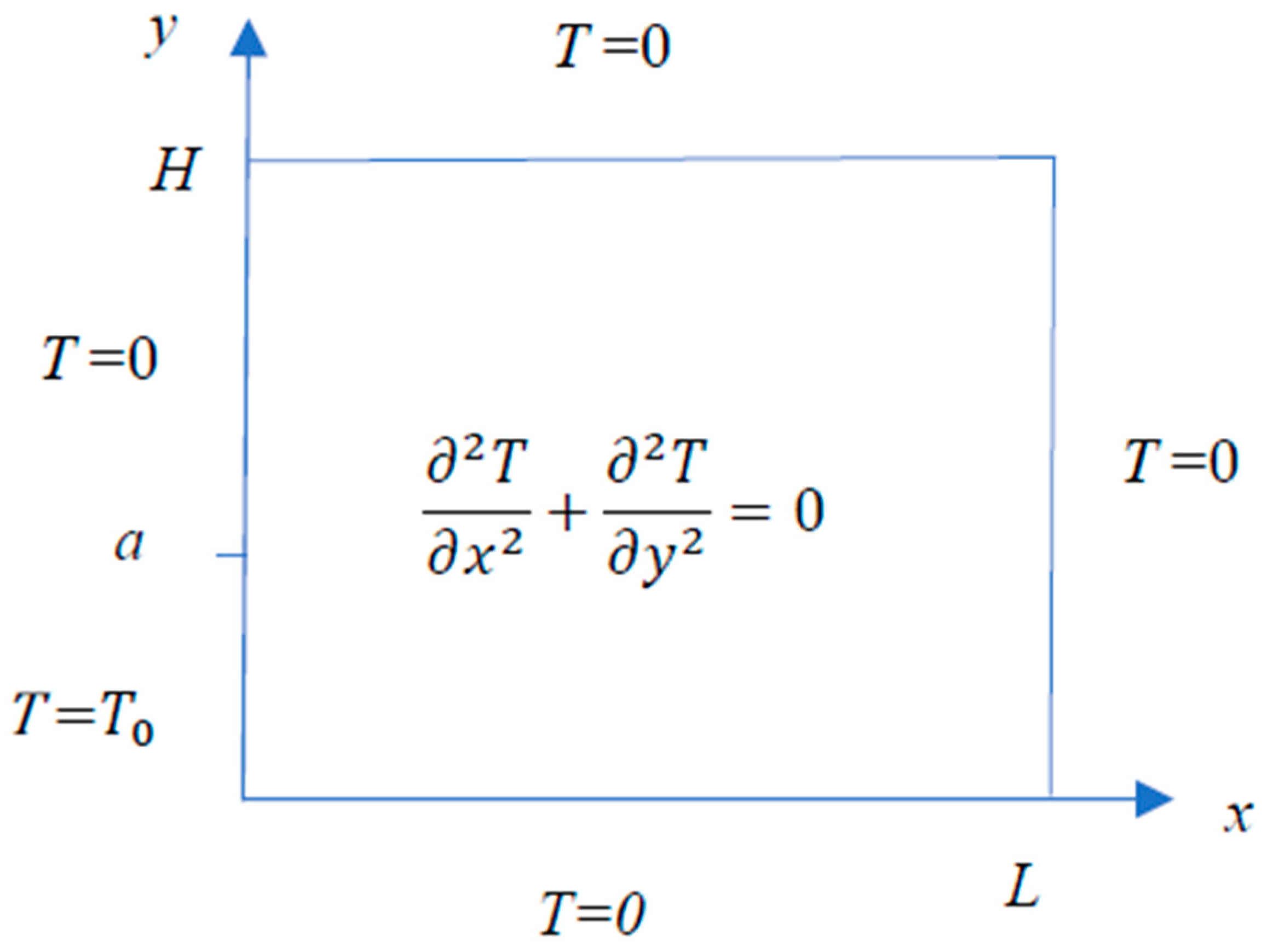
In the finite rectangular domain shown in Figure 1, Laplace’s equation is described as follows:
BCs
where T (x, y) is the temperature in the rectangular domain and T0 is a constant, as shown in Figure 1.

Figure 1.
Laplace’s equation in the rectangular domain.
Figure 1.
Laplace’s equation in the rectangular domain.
Through the method of separation of variables, the general solution for temperature in Equation (1) is easily solved, as shown in Equation (5):
The Fourier coefficient in Equation (5) is calculated based on the BCs (Equations (2)–(4)):
Substituting Equation (6) into Equation (5), we obtain the infinite series solution in the rectangular domain, as follows:
where
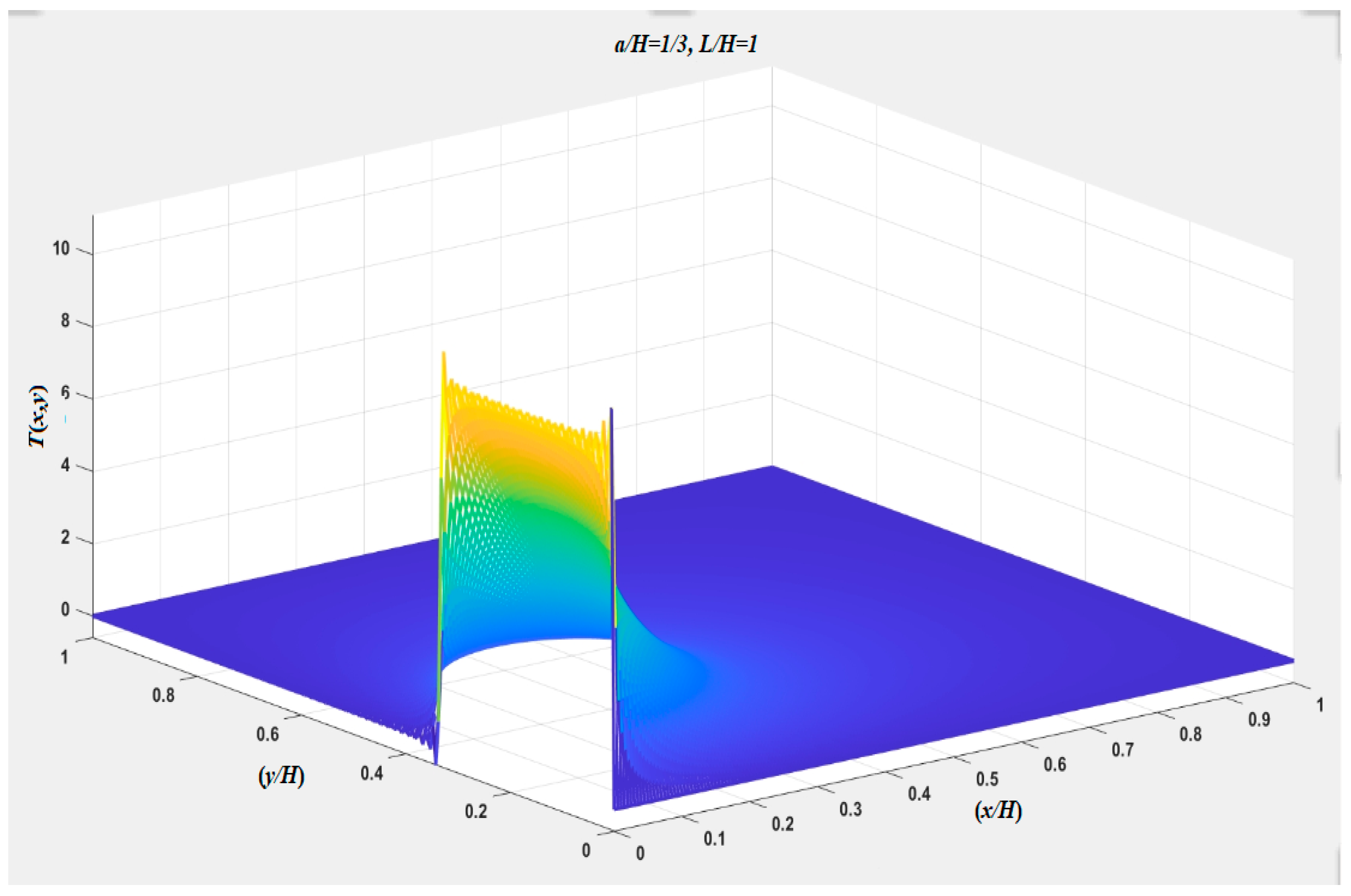
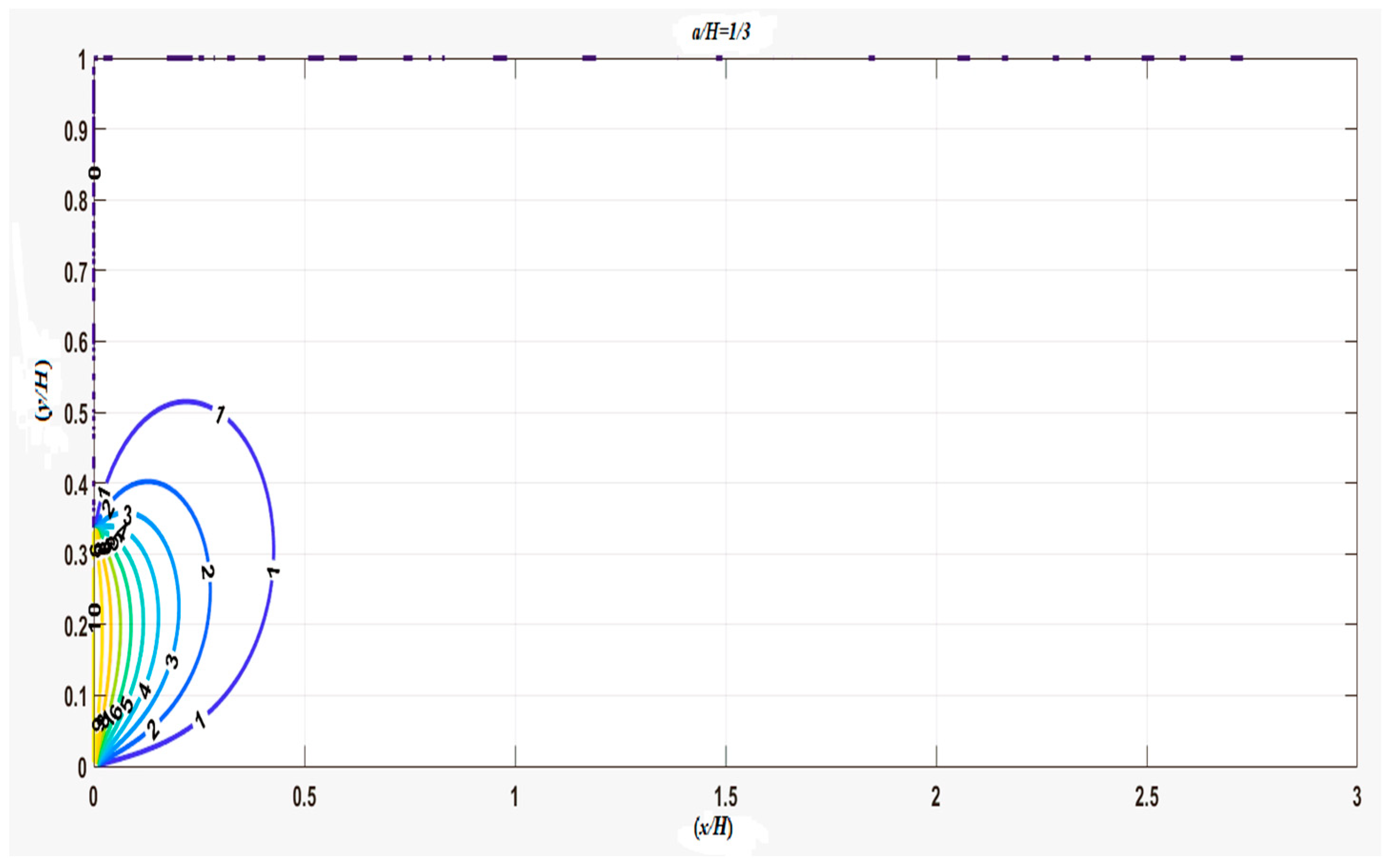
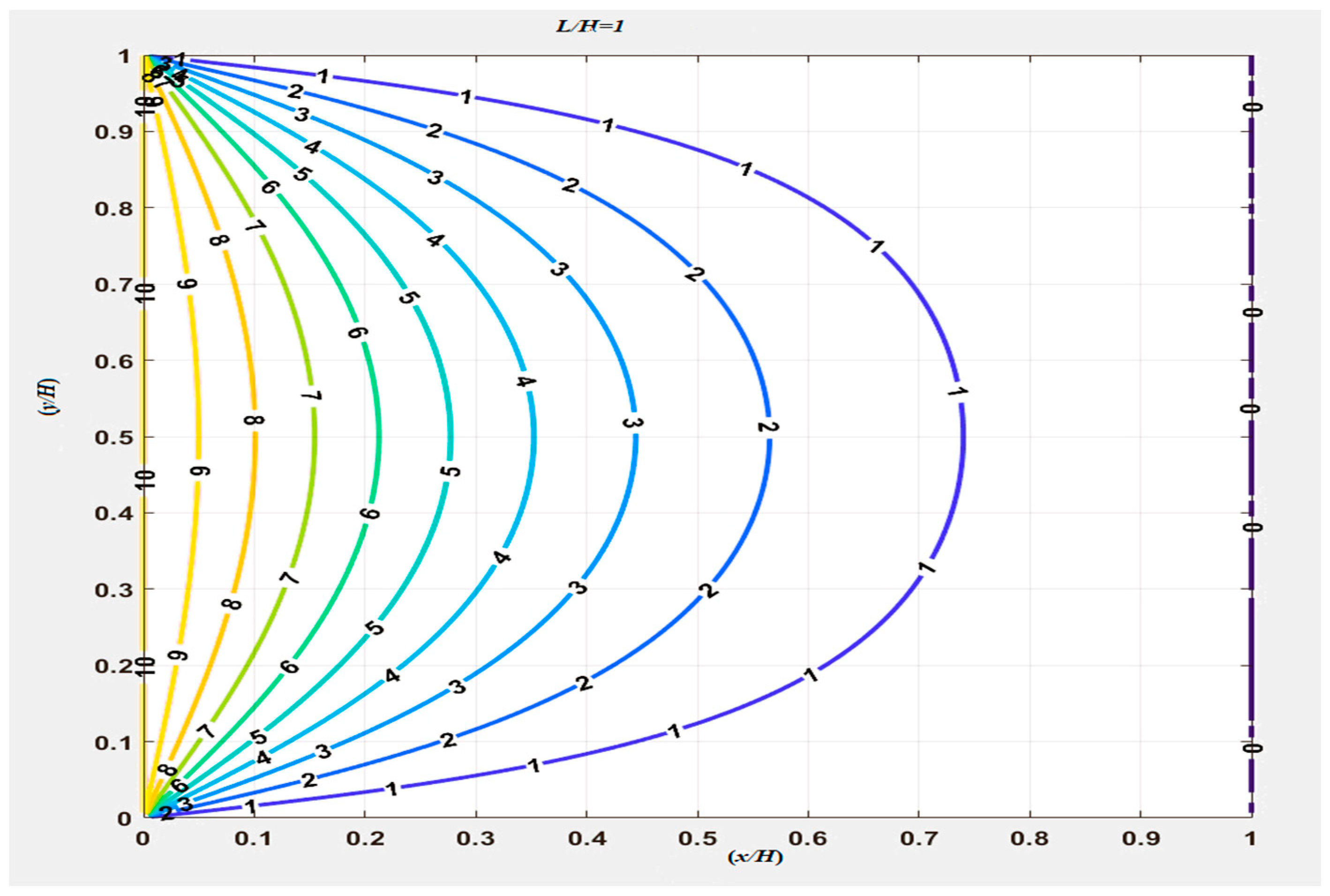
The numerical calculation of the 3D plot from Equation (7) with , is shown in Figure 2, and the 2D distribution from Equation (7) with , is plotted in Figure 3.

Figure 2.
The 3D distribution of temperature from Equation (7) by numerical calculation.
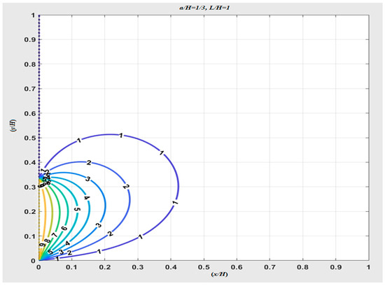
Figure 3.
The 2D distribution of temperature from Equation (7) by numerical calculation.
In Figure 2, showing the calculation of infinite series to find the converged temperature distribution, there is an oscillation phenomenon (the so-called Gibbs’ phenomenon [8]) near the singular points (0, 0) and (0, 1/3).
If , the solution for in Equation (7) is simplified to
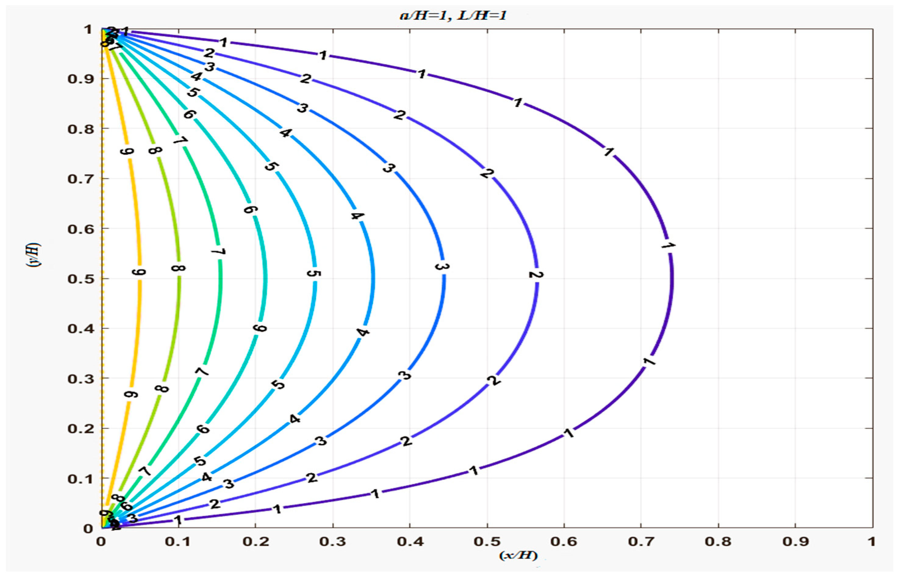
In terms of numerical calculation, the 3D plot of Equation (9) with is shown in Figure 4, and the 2D plot of Equation (9) with is shown in Figure 5.
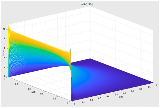
Figure 4.
The 3D distribution of temperature from Equation (9) by numerical calculation.
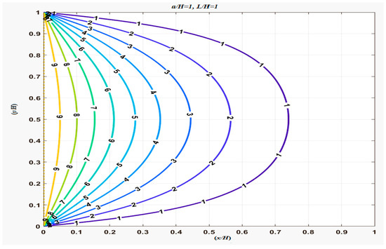
Figure 5.
The 2D distribution of temperature from Equation (9) by numerical calculation.
2.2. Semi-Infinite Strip Domain
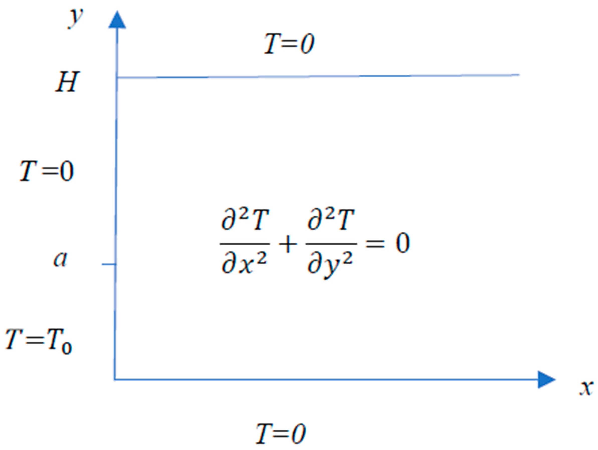
For the semi-infinite strip domain shown in Figure 6, Laplace’s equation in the domain is shown below.
BCs
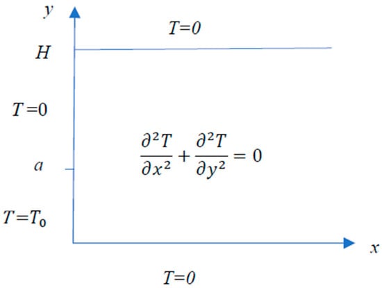
Figure 6.
Semi-infinite strip domain.
Figure 6.
Semi-infinite strip domain.
As the semi-infinite strip length from Equation (8) , the approximate result is found as follows:
When substituting Equation (14) into Equation (7), then the solution can be expressed as follows:
From the trigonometric relation, we have
Then, Equation (15) becomes
Mathematical manipulation [9] yields
Substituting Equations (18) and (19) into Equation (17) yields the closed-form solution, , in a semi-infinite domain for :
The closed-form solution in Equation (20) is unexpectedly complicated, so it is tedious to derive the singular similarity form; meanwhile, the temperature is no more in an infinite series form. The 3D plot of the complicate closed form of the temperature distribution (Equation (20)) with is shown in Figure 7, and the 2D plot of Equation (20) with is shown in Figure 8.
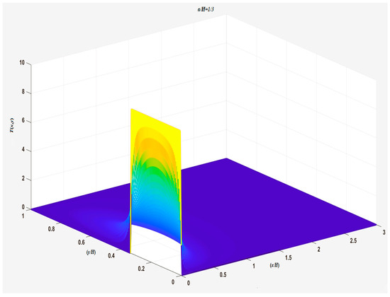
Figure 7.
The 3D distribution of temperature from Equation (20).
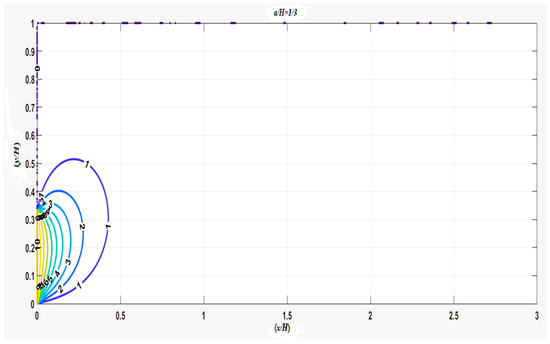
Figure 8.
The 2D distribution of temperature from Equation (20).
As , from Equation (15), the infinite series solution becomes
From Equation (18), the infinite series Equation (21) converges to an exact singular similarity solution, , as follows:
where the similarity variable , and the similarity function satisfies the second-order ordinary differential equation in the following form [10]:
BCs
The singular similarity solution of Equation (23) is shown in Equation (22).
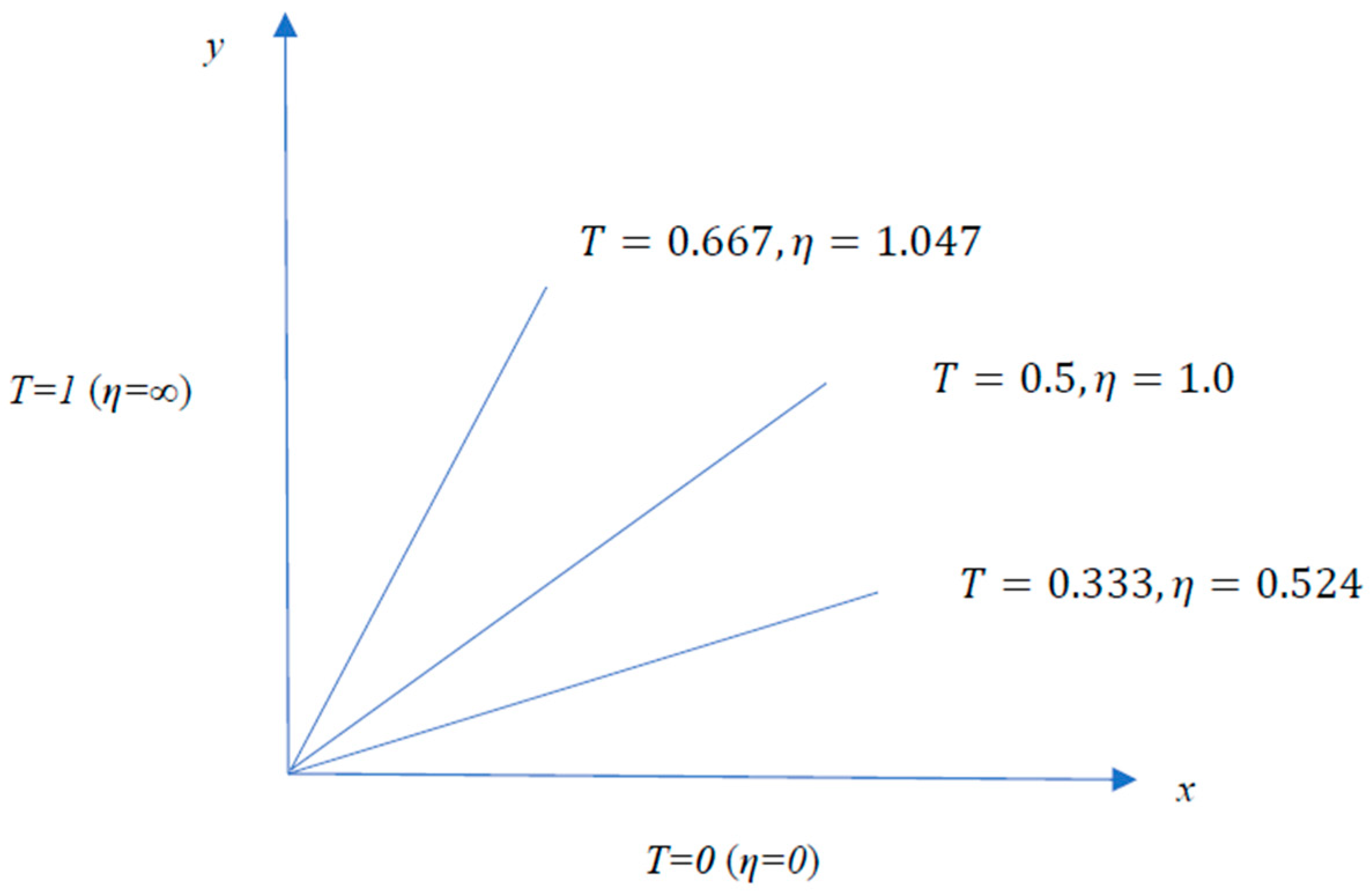
From Equation (22), the dimensionless similarity solution for temperature is
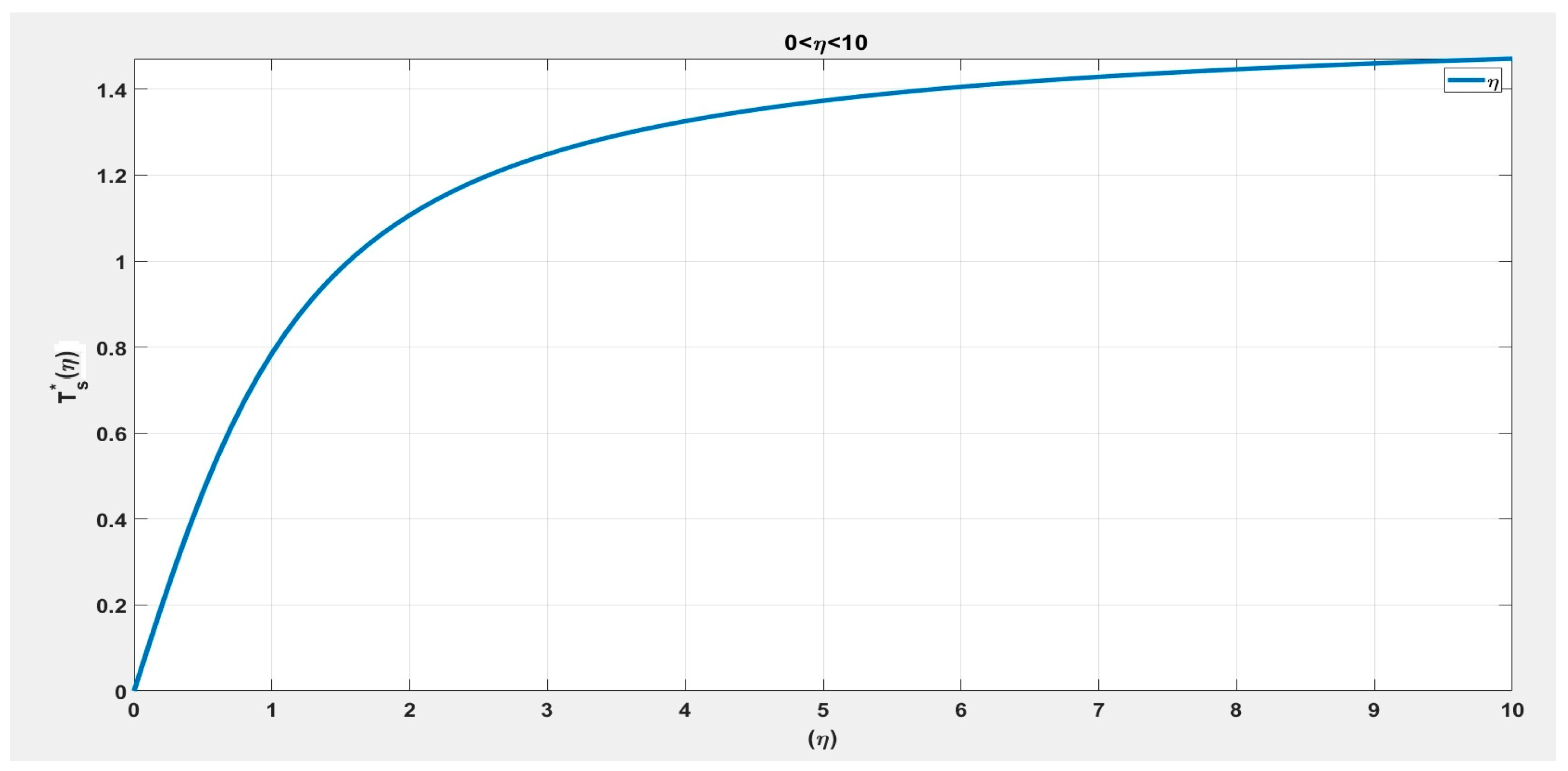
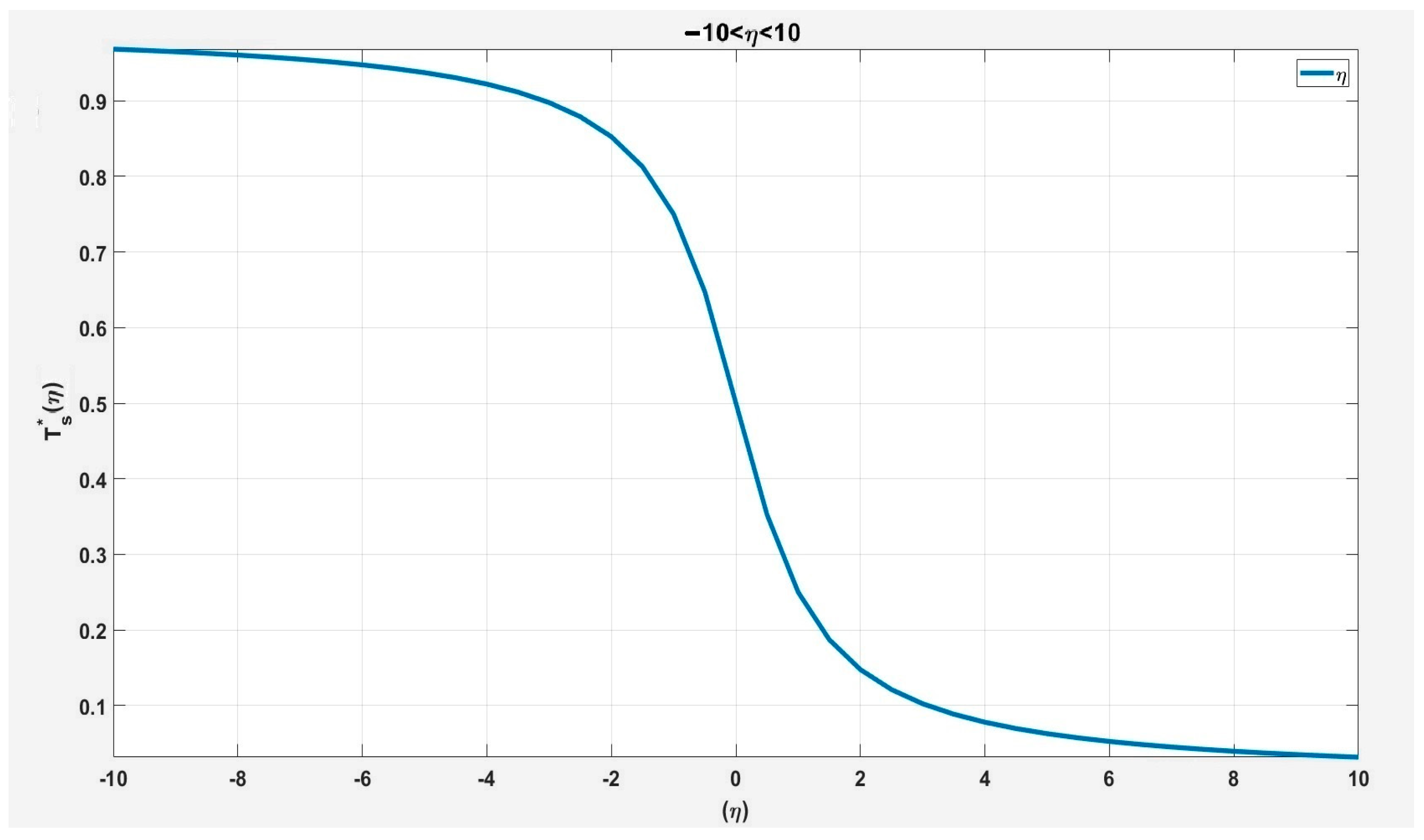
The plot of from Equation (25) is shown in Figure 9 for .
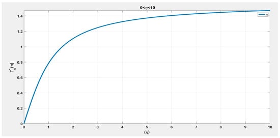
Figure 9.
Dimensionless similarity solution in Equation (25).
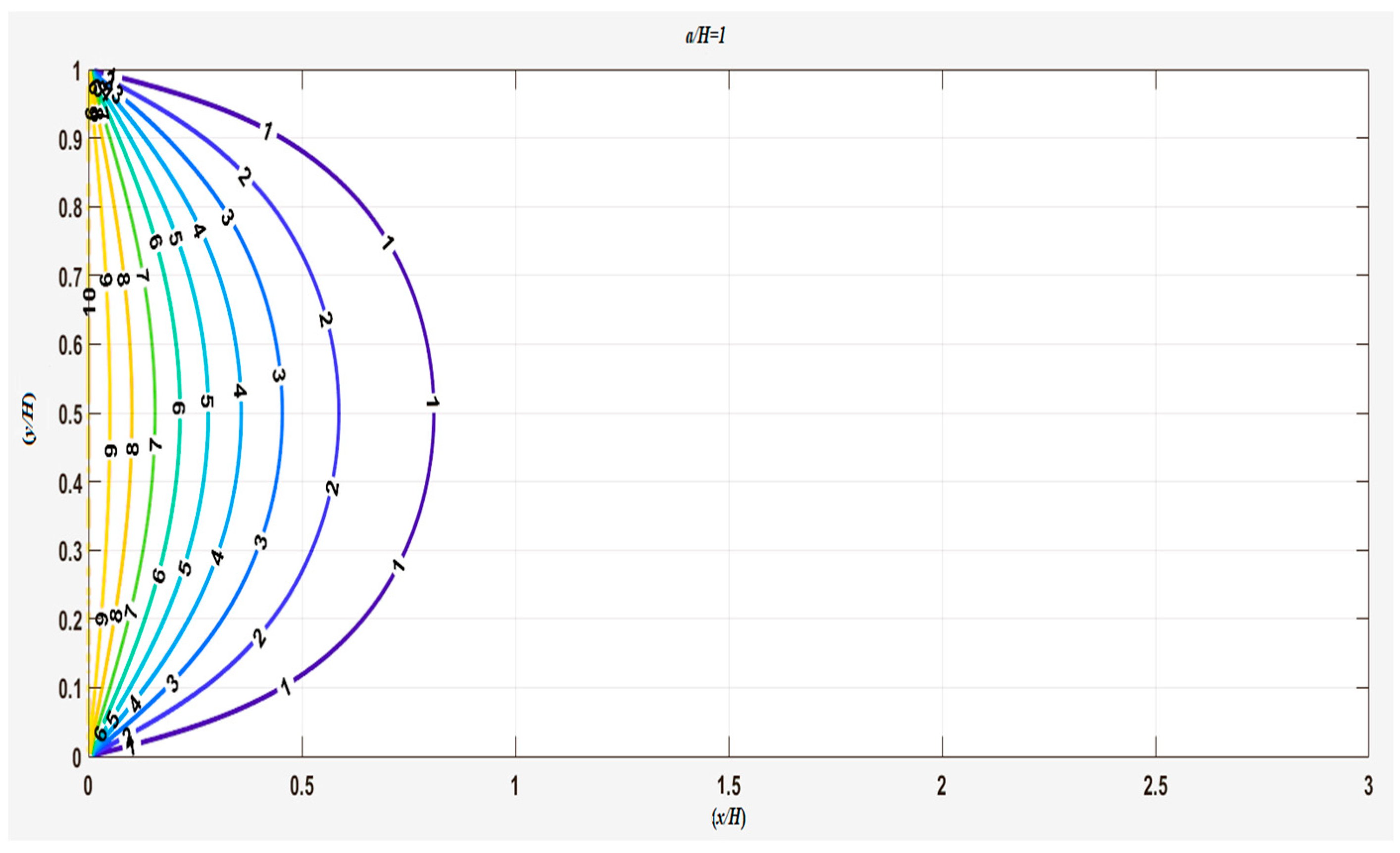
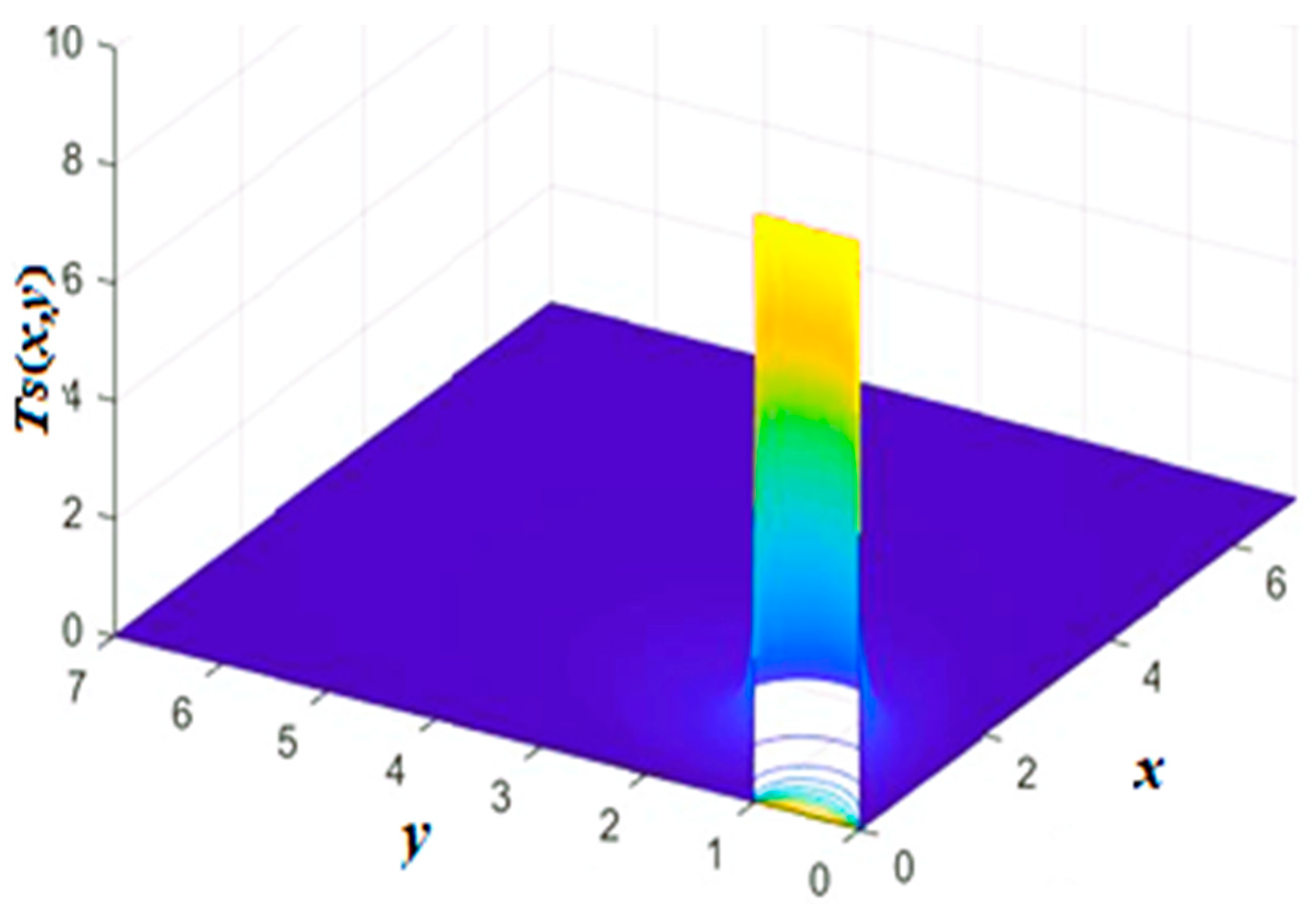
The 3D plot of Equation (22) with is shown in Figure 10, and the 2D plot of Equation (22) with is plotted in Figure 11.
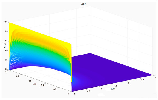
Figure 10.
The 3D distribution of temperature from the closed form of Equation (22).
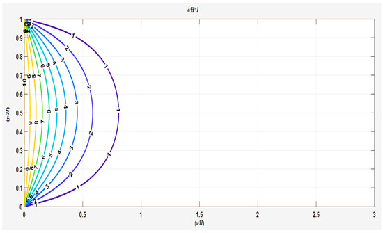
Figure 11.
The 2D distribution of temperature from the closed form of Equation (22).
Note that the singular similarity solution for a semi-infinite strip domain in Equation (22) was confirmed using the method of conformal mapping by Greenberg [9]. In Greenberg’s study, it was proposed that the closed-form solution ascertained through the method of conformal mapping is much superior to the solution in an infinite series form obtained via the method of separation of variables. However, in this study, the singular similarity solution (Equation (22)) was directly derived through the infinite series, a much better approach than using the method of conformal mapping. Also, it is worth mentioning that, in Figure 10, the temperature distribution shows no Gibbs’ phenomenon [8] near the singular points from the singular similarity solution.
It is interesting to point out that the infinite series solution (Equation (9)) in the rectangular domain can be expressed in terms of the singular similarity solution (Equation (22)) in the semi-infinite strip domain. The derivation is shown as follows:
where the reminder solution in the region is expressed as
where the in Equation (27) is
Substituting Equation (28) into Equation (27), for yields
Finally, we obtain the infinite series solution (Equation (9)) of the rectangular domain in terms of similarity solution in Equation (22) of the semi-infinite strip domain as follows:
It is difficult to justify the singular behavior near certain singular points of the rectangular domain from the infinite series (Equation (9)). However, we can express Equation (9) in the similarity form, which is the first term on the right-hand side of Equation (30), subtracting the second term on the right-hand side of Equation (30). As we know, when L→∞, the second term on the right-hand side of Equation (30) will be diminished, and the left-hand side of Equation (30) will be equal to the first term on the right-hand side of Equation (30), as discussed in Equation (18).
The 3D and 2D temperature distributions with the infinite series solution of the left-hand side of Equation (30) are shown in Figure 4 and Figure 5, respectively, and the 3D and 2D temperature distributions of the right-hand side of Equation (30), shown in Figure 12 and Figure 13, can be used to justify the correctness of Equation (30). There is no significant difference in temperature distribution between Figure 4 and Figure 12 except near the singular points (0,0) and (0,1), where Gibbs’ phenomenon from the infinite series solution is shown in Figure 4. Also, when comparing Figure 5 and Figure 13, it can be seen that the 2D projection of temperature distribution is the same.
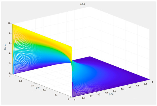
Figure 12.
The 3D temperature distribution from the calculation of the right-hand side of Equation (30).
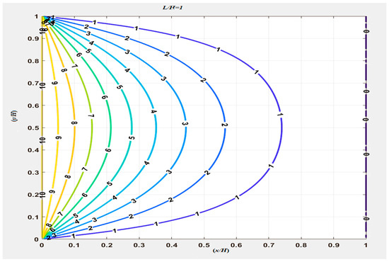
Figure 13.
The 2D temperature distribution from the calculation of the right-hand side of Equation (30).
Moreover, considering the singular behavior near the origin, where , Equation (30) becomes
From (31), it can be proven that for a rectangular domain, there is source-type singular behavior near the origin in Figure 3. In the numerical calculation near that singular point, the convergence is very slow due to the source-type singular behavior in (31). Of course, there is more source-type singular behavior near the singular point at as shown in Figure 5.
2.3. First-Quadrant Domain
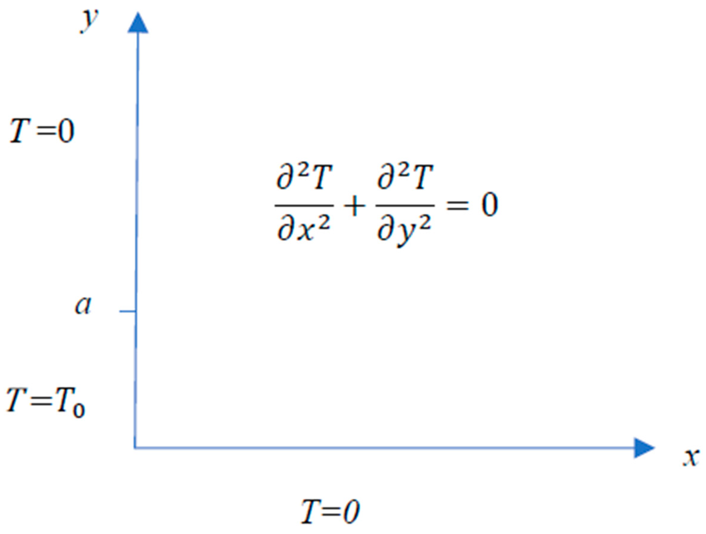
For the first-quadrant domain shown in Figure 14, Laplace’s equation is expressed as
BCs
where T(x, y) is the temperature in the domain, and T0 is a constant.
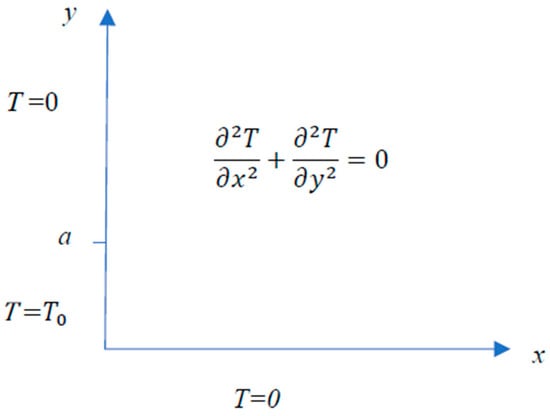
Figure 14.
Laplace’s equation in the first-quadrant domain.
Figure 14.
Laplace’s equation in the first-quadrant domain.
As , from the closed-form solution in Equation (20) of the semi-infinite strip domain, we can find the following forms:
Substituting from Equation (35) to Equation (40) into Equation (20), we obtain the similarity solution in the first-quadrant domain:
From the trigonometric relation, we have
Then, the similarity solution in Equation (43) can be expressed as
where the similarity variable , and the similarity function satisfies the second-order ordinary equation.
BCs
The singular similarity solution of Equation (46) is shown in Equation (45). Then, the dimensionless similarity solution for temperature is
The plot of for Equation (48) is shown in Figure 15 for
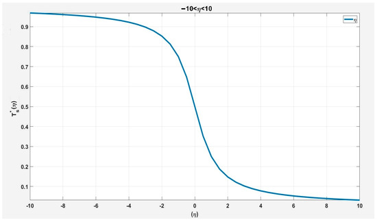
Figure 15.
Dimensionless singular similarity solution, in Equation (48).
The 3D plot of Equation (45) with is shown in Figure 16, and the 2D plot of Equation (45) with is plotted in Figure 17.

Figure 16.
The 3D distribution of temperature from Equation (45).

Figure 17.
The 2D distribution of temperature from Equation (45).
From Equation (43), there is a source-type singular solution near the origin as shown below:
Of course, from Equation (43), there is another source-type singular solution near the singular point as shown below:
The similarity solution (Equation (45)) in the first-quadrant domain can also be solved by the Fourier sine transform [11,12,13].
When comparing Equation (51) with Equation (42), the complicated integral solution in Equation (51) can easily be found analytically as
Carefully investigating the integral solution [14] for Equation (52) yields
The integral results of Equations (53) and (54) can be verified from reference [14].
Now, considering from Equation (43), we also have the following result [13,14]:
As , from Equation (43), we obtain the fundamental singular similarity solution.
with the similarity variable
Near the origin , and from Equation (56), we have
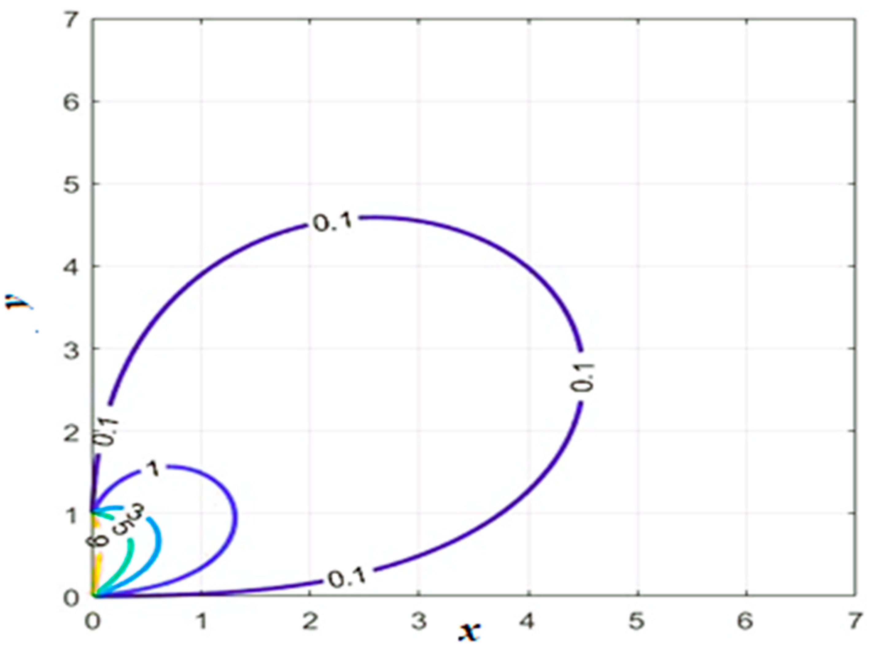
Therefore, there is only one source-type singular solution near the origin in Equation (56) with as shown in Figure 18.
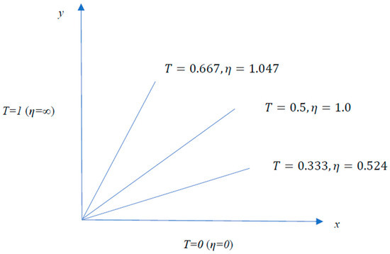
Figure 18.
The 2D contour of the temperature distribution in Equation (56).
Note that the singular similarity solution in Equation (45) for the first-quadrant domain can also be found via Fourier transform and the method of images [13]. However, in this study, it is proven that the analytical singular similarity solution can be derived in a more powerful and easier way through direct application of the basic method of separation of variables for a rectangular domain.
3. Conclusions
The traditional solution to Laplace’s equation for the temperature distribution in a confined domain with discontinuous boundary conditions can be obtained by applying the method of separation of variables. Numerical computation is applied to find the infinite series solution in a very slowly convergent way accompanied by Gibbs’ phenomenon, especially near certain singular points in the domain. In this study, the temperature distribution solutions in terms of the closed form and similarity solution show no oscillation phenomenon near the singular points.
The singular similarity solution derived from the infinite series of the rectangular domain, by extending the domain into a semi-infinite domain, offers a better approach than the closed form of a semi-infinite strip solution obtained through the method of conformal mapping.
By extending the rectangular domain into the first-quadrant domain, the singular similarity solution can be derived from the infinite series solution in a more powerful and direct way than Fourier transform, the method of images, or the method of conformal mapping.
Author Contributions
Conceptualization, C.-K.F. and J.-H.T.; Methodology, C.-K.F. and J.-H.T.; Software, J.-H.T.; Validation, C.-K.F.; Formal analysis, C.-K.F.; Investigation, J.-H.T.; Data curation, C.-K.F. and J.-H.T. All authors have read and agreed to the published version of the manuscript.
Funding
This research received no external funding.
Data Availability Statement
Data are contained within the article.
Conflicts of Interest
The authors declare no conflict of interest.
References
- Carslaw, H.S.; Jaeger, J.C. Conduction of Heat in Solid, 2nd ed.; Oxford University Press: Oxford, UK, 1959. [Google Scholar]
- Kevorkian, J. Partial Differential Equations: Analytical Solution Techniques, 2nd ed.; Springer: New York, NY, USA, 2010. [Google Scholar]
- Myint-U, T.; Debnath, L. Linear Partial. Differential Equations for Scientists and Engineers, 4th ed.; Springer: New York, NY, USA, 2007. [Google Scholar]
- Haberman, R. Applied Partial Differential Equations: With Fourier Series and Boundary Value Problems, 5th ed.; Pearson Education, Pearson Publishing Company: New York, NY, USA, 2013. [Google Scholar]
- Churchill, R.V.; Brown, J.W. Fourier Series and Boundary Value Problems, 3rd ed.; McGraw-Hill: New York, NY, USA, 1978. [Google Scholar]
- Bluman, G.; Cole, J.D. Similarity Method for Differential Equations; Springer: New York, NY, USA, 1974. [Google Scholar]
- Feng, C.K.; Lee, C.Y. The Similarity Analysis of Vibrating Membrane with It’s Applications. Int. J. Mech. Sci. 2005, 47, 961–981. [Google Scholar] [CrossRef]
- Gerald, C.F.; Wheatley, P.O. Applied Numerical Analysis, 7th ed.; Pearson Publishing Company: New York, NY, USA, 2004. [Google Scholar]
- Greenberg, M. Advanced Engineering Mathematics, 2nd ed.; Pearson Education, Pearson Publishing Company: New York, NY, USA, 1998. [Google Scholar]
- Feng, C.K. The General Similarity Solution of Laplace’s Equation with Applications to Boundary Value Problems. In Proceedings of the 1987 EQUADIFF Conference, Xanthi, Greece, 24–28 August 1987; pp. 237–248. [Google Scholar]
- Carslaw, H.S.; Jaeger, J.C. Operational Methods in Applied Mathematics, 2nd ed.; Dover Publications: New York, NY, USA, 1963. [Google Scholar]
- Churchill, R.V. Operational Mathematics, 3rd ed.; Mc-Graw Hill: New York, NY, USA, 1972. [Google Scholar]
- Tang, J.H.; Feng, C.k. A Unified Singular Solution of Laplace’s Equation with Neumann and Dirichlet Boundary Conditions. Appl. Comput. Math. 2022, 1, 38–47. [Google Scholar] [CrossRef]
- Gradshteyn, I.S.; Ryzhik, I.M. Tables of Integrals, Series and Products, 4th ed.; Academic Press: New York, NY, USA, 1965. [Google Scholar]
Disclaimer/Publisher’s Note: The statements, opinions and data contained in all publications are solely those of the individual author(s) and contributor(s) and not of MDPI and/or the editor(s). MDPI and/or the editor(s) disclaim responsibility for any injury to people or property resulting from any ideas, methods, instructions or products referred to in the content. |
© 2024 by the authors. Licensee MDPI, Basel, Switzerland. This article is an open access article distributed under the terms and conditions of the Creative Commons Attribution (CC BY) license (https://creativecommons.org/licenses/by/4.0/).

