Abstract
The threat posed by the COVID-19 pandemic has been accompanied by an epidemic of misinformation, causing confusion and mistrust among the public. Misinformation about COVID-19 whether intentional or unintentional takes many forms, including conspiracy theories, false treatments, and inaccurate information about the origins and spread of the virus. Though the pandemic has brought to light the significant impact of misinformation on public health, mathematical modeling emerged as a valuable tool for understanding the spread of COVID-19 and the impact of public health interventions. However, there has been limited research on the mathematical modeling of the spread of misinformation related to COVID-19. In this paper, we present a mathematical model of the spread of misinformation related to COVID-19. The model highlights the challenges posed by misinformation, in that rather than focusing only on the reproduction number that drives new infections, there is an additional threshold parameter that drives the spread of misinformation. The equilibria of the model are analyzed for both local and global stability, and numerical simulations are presented. We also discuss the model’s potential to develop effective strategies for combating misinformation related to COVID-19.
1. Introduction
COVID-19, also known as the coronavirus disease, caused by the novel coronavirus SARS-CoV-2, has had a profound impact on global health since its emergence in late 2019. The first case was reported in Wuhan, China, and the virus rapidly spread worldwide, with multiple waves of infections observed in different regions. After more than 118,000 cases in 114 countries and 4291 deaths, the World Health Organization (WHO) declared COVID-19 a pandemic on 11 March 2020 [1,2]. COVID-19 is primarily transmitted through respiratory droplets when an infected individual coughs, sneezes, talks, or breathes heavily in close proximity to others [3]. It exhibits a wide spectrum of clinical manifestations, ranging from mild flu-like symptoms to severe respiratory distress and multi-organ failure [4,5]. Several factors including social behavior have influenced the disease’s transmission dynamics. COVID-19 continues to evolve, with variations in the prevalence and severity of the disease due to emerging variants, vaccination campaigns, and public health measures implemented by governments and health organizations. Globally, as of 27 September 2023, there have been 770,875,433 confirmed cases of COVID-19, including 6,959,316 deaths, reported to the WHO [6].
During the pandemic, many countries put in place a series of measures to contain the spread of COVID-19, such as social distancing, masking, self-quarantine and eventually vaccinations when they became available, which essentially helped to regulate the transmission of the coronavirus disease. However, the lack of clear and concise messaging from public health officials also contributed to the spread of misinformation related to COVID-19. The constantly evolving nature of the pandemic and the lack of understanding of the virus early on led to conflicting information and messages from public health officials, leading to confusion and mistrust among the public. This led some individuals to turn to alternative sources of information, including misinformation, for guidance.
Misinformation related to COVID-19 has taken various forms [7,8,9]. Conspiracy theories related to COVID-19 have been widely circulated, often claiming that the virus was intentionally created and spread as a bioweapon or part of a global plot [10]. For example, the theory that 5G technology is responsible for the spread of COVID-19 has been shared widely on social media platforms, despite the lack of scientific evidence to support this claim [11]. False treatments and cures for COVID-19 have also been promoted, leading to dangerous consequences for individuals who follow them. For instance, the use of disinfectants, such as bleach, to treat COVID-19 has been widely reported, leading to severe injuries and deaths [12]. False claims that certain drugs, such as hydroxychloroquine, are effective in treating COVID-19 have also been circulated, leading to hoarding and shortages of the drug, which is actually not effective in treating the virus [13]. Rumors about the origins and spread of COVID-19 have also contributed to the misinformation landscape surrounding the disease. For example, the theory that the virus was intentionally created and spread by China has been promoted by some media outlets and politicians, despite the lack of evidence to support this claim [10]. Furthermore, misinformation surrounding vaccines includes unfounded allegations of adverse effects, doubts about their efficacy, and baseless theories about secret agendas. Such misinformation undermines public trust in vaccines, leading to vaccine hesitancy and jeopardizing the achievement of widespread vaccination coverage. The politicization of the pandemic also contributed to the spread of misinformation related to COVID-19. Political leaders and media outlets have often taken polarizing stances on the pandemic, leading to the amplification of misinformation and conspiracy theories [14]. This led to a lack of consensus on the severity of the pandemic and the efficacy of public health measures, further contributing to the spread of misinformation.
Mathematical models have been used extensively to understand the spread of COVID-19 and to inform public health interventions [15]. Several of these models typically involve a set of differential equations that describe the dynamics of the virus spread, including the number of infected individuals, the rate of transmission, and the effectiveness of interventions such as social distancing and vaccination [16,17]. Mathematical models can be used to estimate key parameters of the pandemic, such as the basic reproduction number (), which measures the average number of people infected by each infected individual in a susceptible population [18]. By estimating , mathematical models can be used to predict the potential impact of different interventions and to guide public health policy.
There are many challenges associated with modeling COVID-19, including the uncertainty of key parameters, such as the transmission rate, the duration of infectiousness, and the duration of immunity after recovery or vaccination [19,20]. In addition, the complex dynamics of the pandemic, including the emergence of new variants and changes in public behavior due to misinformation, made it difficult to predict the course of the pandemic accurately. In this study, we will present a mathematical model of the role of misleading information in the transmission dynamics of COVID-19 since misinformed individuals were likely to ignore measures such as social distancing, masking, vaccinations and others, put in place to safeguard the population. The model is based on the assumptions that some proportion of the population is vulnerable to misinformation. We refer to misinformation as false or inaccurate information that is spread, either intentionally or unintentionally, leading to a distortion of facts or a misunderstanding of reality. It can be disseminated through various channels, including social media, news outlets, word-of-mouth, or online platforms. Misinformation can take different forms, such as misleading statements, fabricated data, conspiracy theories, or misinterpretations of legitimate information. It often aims to deceive or manipulate individuals, resulting in harmful consequences, including the erosion of trust, the promotion of fear and panic, the hindrance of informed decision-making, and potentially detrimental effects on public health, social cohesion, and democratic processes.
The purpose of this study is to assess the impact that the amount of misinformation circulating has on the transmission dynamics of COVID-19 in a population. To achieve this goal, we formulated an SIR type model with an extra compartment representing individuals that have been misled through misinformation. Because there was abundant misinformation (whether intended or unintended) associated with COVID-19, the model presented also treats the quantity of misinformation as a state labeled M based on the assumption that it is synthesized by mislead individuals. This approach is similar to target cell models where virions are produced by infected cells [21]. The equilibrium solutions of the model are obtained using computed threshold parameters and their stability established both analytically and numerically. Simulations of the model indicate that COVID-19 will significantly affect a population negatively if misinformation is not properly tackled.
2. Mathematical Model
The model presented below is an SIR model in nature with additional compartments for misinformed individuals, deaths, and the density of misleading information circulating. We assume that as the susceptible population comes into contact with circulating false or inaccurate information spreading among a community, some will be misled at a rate of and move into the misinformed compartment . Irrespective of the medium through which it is disseminated, we assume that at any point in time , circulating misinformation is the sum total of all forms, including misleading statements, fabricated data, conspiracy theories, or misinterpretations of legitimate information. We assume that misinformation is generated at a rate by people that are already misinformed or bad actors who we also categorized as misinformed, and we suppose that misleading information density decays at the rate . The model therefore assumes that misleading information is only generated by individuals in the compartment. We also assume that misled individuals through awareness campaigns or other sources reject false information recover at a rate and move back into the susceptible compartment. Interactions between susceptible and misinformed individuals with COVID-19 infected individuals lead to infections, respectively, at rates and . We assumed that infected individuals either recovered at the rate or died from a COVID-19 related complication at the rate . It is further assumed new individuals are recruited only as susceptibles at some rate and that the natural death rate in all compartments is . A schematic diagram of the model is given in Figure 1, and a summary of parameters and their description is given in Table 1.
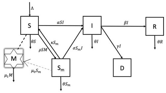
Figure 1.
Schematic diagram of COVID-19 transmission with misinformation. Individuals transition from compartments S and to compartment I as a result of their interaction with individuals in compartment I. Individuals transition between compartments S and as a result of interaction with misinform M (either by consuming it or recovering from it). Misinformation density is produced by individuals in compartment .

Table 1.
Description of model parameters.
Taking into consideration the assumptions stated above and illustrated in the schematic diagram, the system of differential equations that governs the model is as follows:
where we have assumed that all the parameter values are positive and the initial conditions , , , , , and are all non-negative. We note that at the start of the outbreak, and
Before proceeding, we observe that the equation for COVID-19 deaths , that is Equation (5), is decoupled from the rest of the system and therefore will be neglected in all subsequent analyses. We start by exploring the basic dynamical features of the model. In particular, we establish the positivity of solutions of the model and an invariance space. The following result shows that the model always admits positive solutions.
Theorem 1.
Let the initial conditions of the model be , , , , and . Then, the solutions of the model with positive initial conditions, will remain positive for all time t > 0.
Proof.
We start by dividing Equations (1)–(4) and (6), respectively, by the variables S, , I, R, and M. Integrating the resulting differential equations on the time interval , and applying the initial conditions, we obtain the following expressions:
,
,
,
, and .
Since the initial conditions are non-negative, it is obvious from the above expressions that , , , , and are always positive for all times where . Thus, the solution of the model with stated initial condition is always positive. □
Next, we show that the solution of the model is bounded. With the given condition, we consider the living population defined by and show that and are bounded in the following result.
Theorem 2.
If the initial conditions of the model satisfy and , then the solution of the model is bounded.
Proof.
Since , and from Theorem 1, it is obvious that is bounded from below, and therefore, . It only remains to establish that is bounded from above. Differentiating and substituting the derivatives from the model, we obtain the differential equation
from which we obtain the differential inequality
whose solution satisfies
It is evident from the above inequality that the living population of the system is always bounded from above. Further, we observe from the inequality that if the initial condition , then we have that as is a strict upper bound.
To conclude boundedness of the model, we also established that the misinformation density is bounded. We already showed in Theorem 1 that is always positive, that is, , thus it is bounded from below. For boundedness from above, we consider the case when . Since , we must have that . Using the differential equation for misinformation density, we obtain the differential inequality
whose solution satisfies
Clearly, the information density is bounded from above. Similarly, if , then we have that as a strict upper bound. □
Lemma 1.
The closed set
is positively invariant and attracting for the model.
Proof.
The proof follows directly from Theorems 1 and 2 where the trivial existence and uniqueness of solution is assumed. □
3. Analysis of the Model
In this section, we compute the equilibria and provide conditions for their existence. We also provide the reproduction number of the model and use it to study the stabilty of the computed equilibria. Note also that the equation for the recovered is decoupled from the rest of the system, in addition to that for deaths . We will therefore ignore these equations in the subsequent analysis given that their behavior can easily be deduced given the behavior of the remaining sub-system.
3.1. Existence of Equilibria
By decoupling the equations for R and D, the equilibria of the model is given by the solution of the sub-system
Since the last equation above only depends on variable , can be represented as
From the third equation in the sub-system, we see that either which leads to the disease-free equilibrium (DFE) of the model, or , which leads to the Endemic Equilibrium.
Suppose that denotes a DFE, then further computation yields two DFEs,
We note here that the second DFE will only exist if .
Before going further into the analysis, we pause and compute the reproduction number, , of the model. The reproduction number is the number of secondary infections that occur when an infectious person is put into a completely susceptible population. Using the next generation matrix method (see for example Duatel et al. [22]) and the DFEs, and , respectively, we obtain the reproduction numbers
We remark here that regulates the model in the absence of misinformation, while drives the model when misinformation is persistent.
We now turn our attention to establish the endemic equilibria of the model. Suppose that denotes an endemic equilibrium, then using equation and the necessary equations in the sub-system, we obtain two endemic equilibria namely,
and
where and where
We also remark here that the first endemic equilibrium exists if , and the second endemic equilibrium exists if and .
3.2. Stability of Equilibria
In this section, we establish local stability results for the DFEs and endemic equilibria obtained above under appropriate conditions. We begin by noting that the Jacobian matrix, , of the sub-system is given by
Theorem 3.
If and , then the DFE is locally asymptotically stable, otherwise it is unstable.
Proof.
Evaluating the Jacobian matrix at the DFE , we obtain
whose characteristic polynomial is
yeilding the eigenvalues
From the above, it is obvious that and have negative real parts, since and can be rewritten as
Thus, if , then . has a negative real part if
holds true. Therefore, if and , then the DFE is locally asymptotically stable, otherwise it is unstable if . □
We now conclude our analysis of the first DFE by establishing a global stability result. For this purpose, we recall establishing in Section 2 that at any time t, the living population is bounded above and satisfies
where . The following results are a consequence of the above inequality.
Lemma 2.
The living population at all times t.
The following result provides global stability for the first DFE , that is, when there is no COVID-19 and there is also no misinformation.
Theorem 4.
In view of Lemma 2, if , and if , then the first disease-free equilibrium, is globally asymptotically stable, otherwise it is unstable.
Proof.
In order to prove Theorem 4, we consider Lyapunov function candidate . Taking its derivative we obtain,
Since the model assumes that , then the above equation becomes
If then by Lemma 2, we obtain that . Thus, we obtain the differential inequality
It is clear that if , then and therefore, by LaSalle’s invariance principle the disease-free equilibrium is globally asymptotically stable [23]. □
Next, we consider the local stability of the second DFE and state the following result.
Theorem 5.
If and , then the DFE is locally asymptotically stable, otherwise it is unstable.
Proof.
Evaluating the Jacobian matrix at the the second DFE, that is, , we obtain the Jacobian matrix
Clearly, we see from the third row of the above matrix that
The remaining factor of the characteristic polynomial is of degree three and is given by
where
To establish that the remaining eigenvalues (that is the zeros of the above cubic equation) have negative real parts, we use Routh–Hurwitz criterion. It is obvious from the above coefficients , , and that if the condition is satisfied then , , and . Further, we also see that the inequality
holds true. Since , , and are all positive and , we conclude using Routh–Hurwitz criterion that the remaining eigenvalues have negative real parts. Therefore, if , the DFE, , is locally asymptotically stable, otherwise, it is unstable. □
Remark 1.
Just as a reminder, we recall here that the condition was imposed to ensure that the DFE is valid.
Theorem 6.
If , then the Endemic Equilibrium, , is locally asymptotically stable, otherwise it is unstable.
Proof.
Evaluating the Jacobian matrix at the endemic equilibrium , that is, at where , we obtain the Jacobian matrix
The characteristic polynomial is
and the eigenvalues are
From the results above, the eigenvalues and clearly are always negative real numbers or have negative real parts, since . Therefore, we can conclude that if , then the endemic equilibrium, , is locally asymptotically stable and unstable if . □
Remark 2.
We note here that in a similar manner to Theorem 6, it can be established that if , then the endemic equilibrium
where , , and is locally stable.
4. Results and Discussion
In this section, we present numerical simulations of the model under different circumstances focusing on the population of the United States. We simulate the number of infections for different rates related to misinformation and in some instances the number of cumulative deaths. The parameter values used in the simulations were chosen based on values from the published literature for COVID-19 [20,24,25,26] where available and other parameter values were assumed to explore the behavior of the model. The initial conditions were chosen to reflect the United States population of approximately 335 million by setting . Considering that the true population of the US is estimated to range between 331 million and 341 million, we carried out several simulations with small perturbations in the initial conditions and the long term behavior of the model’s predictions did not change.
In the previous section, we established several qualitative results relating to the equilibria of the model. We start by confirming these results numerically in Figure 2, Figure 3 and Figure 4.
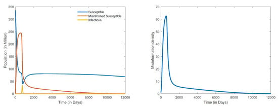
Figure 2.
Numerical simulation of the first DFE: populations distribution (left) and information density (right), for parameter values , , , , , , , , , and .
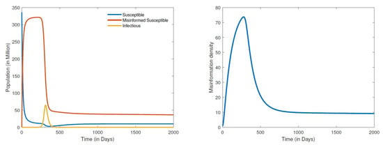
Figure 3.
Numerical simulation of the second DFE: populations distribution (left) and information density (right), for parameter values , , , , , , , , , and .
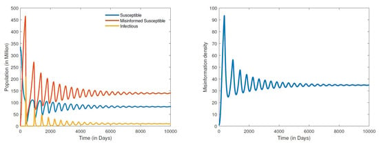
Figure 4.
Numerical simulation of a stable endemic equilibrium: populations distribution (left) and information density (right), for parameter values , , , , , , , , , and .
The results in Figure 2 demonstrate the global stability of the first DFE. The simulations show the disease, the misinformed and the density of misinformation eventually dying out with the passage of time. It is important to observe from these results that though COVID-19 may die out much earlier, it takes much longer for both the misinformed and misinformation density to be eradicated. We note here that the numerical computations for the first DFE were obtained by setting the recovery rate of misinformed individuals () to about 20 times the rate at which susceptible people are misled (). When the recovery rate of misinformed individuals is set at about two times the rate at which the susceptible become misled, we obtained the simulations given in Figure 3. Clearly, the results in Figure 3 demonstrate the second DFE that we also established in the previous section. These results show that even if COVID-19 completely dies out, misinformation about the disease will never go away. Conspiracy theories such as the origin of COVID-19, the disease being a bioweapon, misconceptions about COVID-19 vaccines, and COVID-19 deniers are likely to persist for a long while given the ease and speed at which misinformation is currently disseminated.
The results for the disease-free equilibria discussed above were obtained by assuming a closed population (), that is, no new individuals are entering the community. This is a scenario where there is either strict lockdown or restriction of movement. This was indeed the case with the early variants of COVID-19 where cities/countries were able to restrain the spread of the disease through strict lockdowns; however, misinformation could not be contained. By shifting the paradigm from a closed population to an open one where there is freedom of movement with people entering and leaving the community, the dynamics quickly shift to simulations of an endemic equilibrium. The results in Figure 4 show a globally stable endemic equilibrium. Recall that setting the recovery rate () of misinformed individuals to about 20 times the rate at which susceptible people are misinformed () led to a DFE. However, for an open population where the recruitment rate and , we obtain an endemic equilibrium Figure 4. A further increase in the recovery rate of misinformed individuals say by a multiple of 50 times the rate at which susceptible people are misinformed, that is, , leads to a hopf bifurcation that renders the endemic equilibrium unstable as demonstrated in Figure 5. It is worth noting that the bifurcation here transforms a stable equilibrium to an unstable one containing a very large amplitude of oscillations. We can therefore infer from the results in Figure 4 and Figure 5 that it is not enough to refute misleading information through fact checking by the media. Refuting and also correctly educating the public about COVID-19 should be carried out simultaneously. Media literacy is also essential in combating misinformation related to COVID-19. Increased media literacy can help individuals identify and distinguish between credible sources of information and misinformation. An educated public that is less susceptible to being misled will lead to a better outcome in eradicating COVID-19 or controlling the spread of the disease in an endemic state. We remark here that all simulations that we carried out for a positive recruitment rate, that is (irrespective of how small the value of ), led to an endemic equilibrium. As a consequence, considering the fact that we live in an open population with freedom of movement, COVID-19 will become endemic.
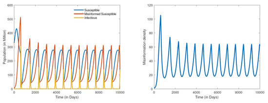
Figure 5.
Numerical simulation of an unstable endemic equilibrium: populations distribution (left) and information density (right), for parameter values , , , , , , , , , and .
Next, we turn our attention to simulate the effect that varying the recovery rate of misinformed individuals () will have on the number of COVID-19 cases and cumulative deaths. The results for the number of COVID-19 cases for a closed population are depicted in Figure 6. We observe here that an increase in the recovering rate of the misinformed () leads to fewer cases of COVID-19. The larger the recovery rate (), the further it takes for the number of cases to peak, and the magnitude of the peak is also smaller. We also note that because it takes longer to peak given a larger recovery rate (), precious time is afforded that can be used by public health officials to implement other measures so as to further reduce the impact of the disease on the entire population. The results in Figure 7 show the cumulative deaths from COVID-19 for different misinformed recovery rates for a closed population. It is also evident from these simulations that a higher recovery rate will lead to a lower number of cumulative COVID-19 deaths. According to the WHO [6], there were about 1,127,252 COVID-19 deaths reported in the United States between 3 January 2020 and 21 September 2023. We observe from the cumulative death simulations in Figure 7 that the rate at which misinformed people recover for the United States is less than five times the rate at which people were misled. Considering that misinformed people contribute to the growth of misinformation, the United States recovery rate of misled individuals appears to be small.
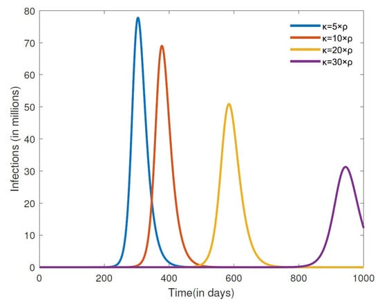
Figure 6.
Numerical simulation of the number of infections for different misinformed recovery rates . The other parameter values are fixed at , , , , , , , , and .
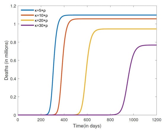
Figure 7.
Numerical simulation cumulative deaths for different recovery rates . The other parameter values are fixed at , , , , , , , , and .
Finally, we consider the effects of misinformation density growth and decay rates on the number of COVID-19 cases, focusing on a closed population. The results in Figure 8 are for different growth rates , while those in Figure 9 are for different decay rates . We can clearly see from the results in Figure 8 that lowering the growth rate of misinformation density leads to fewer cases of COVID-19. Indeed, keeping the growth rate low also leads to a smaller infection peak that occurs further down the road, thus affording time that can be used to implement other containment strategies and consequently minimize the disease burden. Promoting accurate information is essential in combating misinformation related to COVID-19. Public health officials and credible sources of information should provide clear and concise messaging about the virus and public health measures, including vaccination. Positive messaging slows down the growth rate of misinformation. On the other hand, increasing the decay rate of misinformation likewise leads to a smaller infection peak that occurs much later in time. Fact-checking mechanisms can be implemented to combat misinformation related to COVID-19. TV, radio, and social media platforms can implement fact-checking mechanisms to flag and remove misinformation related to the disease.
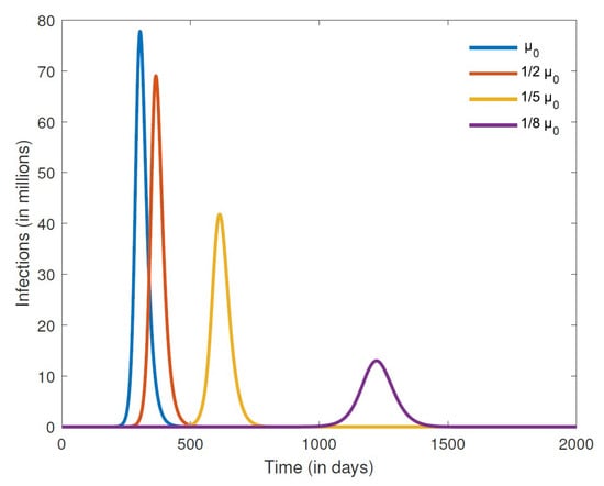
Figure 8.
Numerical simulation of the number of infections for different misinformation growth rates . The other parameter values are fixed at , , , , , , , , and .
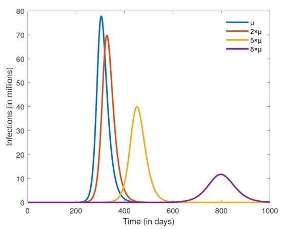
Figure 9.
Numerical simulation of the number of infections for different misinformation decay rates . The other parameter values are fixed at , , , , , , , , and .
5. Conclusions
The COVID-19 pandemic has brought the issue of misinformation to the forefront, highlighting the significant impact on public health. Misinformation can undermine efforts to control the spread of the virus and thus lead to a range of negative consequences, including increased vaccine hesitancy, non-compliance with public health measures, and mistrust of public health officials. In this paper, we formulated a model that captures the transmission dynamics of COVID-19 simultaneously with the spread of misinformation in a community. Analysis of the model shows that it has two disease-free equilibria, one containing misinformation and the other does not. The DFE with no misinformation yields a reproduction number and is both locally and globally stable if . The DFE containing misinformation yields a threshold parameter that renders the equilibrium stable if the value of the parameter is less than one.
Factors contributing to the spread of misinformation related to COVID-19 include the rapid spread of information through social media, the echo chamber effect, and the politicization of the pandemic. When the model is applied to the population of the United States, simulations of cumulative deaths suggest that the United States did a poor job at combating misinformation related to COVID-19. Numerical simulations of the model suggest that a multi-faceted approach is needed to combat the spread of misinformation and promote accurate information about the pandemic. Strategies to combat misinformation related to COVID-19 include promoting accurate information, increasing media literacy, and implementing fact-checking mechanisms. Further, simulations of the model predict that as long as people are able to enter and exit a community, the COVID-19 virus will remain endemic in such a community.
In conclusion, we have shown that mathematical modeling can play an important role in understanding the spread of misinformation related to COVID-19 and developing effective strategies for combating misinformation. Combating COVID-19 misinformation is essential for promoting public health and controlling the spread of the virus. Further, addressing the underlying causes of the spread of misinformation is essential, as is promoting accurate information, increasing media literacy, and implementing fact-checking mechanisms.
Author Contributions
Conceptualization, Z.S. and E.A.; methodology, Z.S. and E.A.; software, Z.S. and E.A.; validation, Z.S. and E.A.; formal analysis, Z.S. and E.A.; investigation, Z.S. and E.A.; resources, Z.S. and E.A.; data curation, Z.S. and E.A.; writing—original draft preparation, Z.S. and E.A.; writing—review and editing, Z.S. and E.A.; visualization, Z.S. and E.A.; supervision, E.A.; project administration, E.A.; funding acquisition, E.A. All authors have read and agreed to the published version of the manuscript.
Funding
This research received no external funding.
Institutional Review Board Statement
Not applicable.
Informed Consent Statement
Not applicable.
Data Availability Statement
Data are contained within the article.
Conflicts of Interest
The authors declare no conflicts of interest.
References
- WHO Director-General’s Opening Remarks at the Media Briefing on COVID-19—11 March 2020. Available online: https://www.who.int/director-general/speeches/detail/who-director-general-s-opening-remarks-at-the-media-briefing-on-COVID-19---11-march-2020 (accessed on 1 January 2023).
- Cucinotta, D.; Vanelli, M. WHO Declares COVID-19 a Pandemic. Acta Biomed. 2020, 91, 157–160. [Google Scholar] [CrossRef] [PubMed]
- Centers for Disease Control and Prevention. Available online: https://www.cdc.gov/coronavirus/2019-ncov/science/science-briefs/sars-cov-2-transmission.html (accessed on 1 January 2023).
- Centers for Disease Control and Prevention. Available online: https://www.cdc.gov/coronavirus/2019-ncov/symptoms-testing/symptoms.html (accessed on 1 January 2023).
- da Rosa Mesquita, R.; Francelino Silva Junior, L.C.; Santos Santana, F.M.; Farias de Oliveira, T.; Campos Alcântara, R.; Monteiro Arnozo, G.; Rodrigues da Silva Filho, E.; Galdino dos Santos, A.G.; Oliveira da Cunha, E.J.; Salgueiro de Aquino, S.H.; et al. Clinical manifestations of COVID-19 in the general population: Systematic review. Wien Klin Wochenschr. 2021, 133, 377–382. [Google Scholar] [CrossRef] [PubMed]
- World Health Organization. Who Coronavirus (COVID-19) Dashboard. Available online: https://covid19.who.int/ (accessed on 1 October 2023).
- Suarez-Lledo, V.; Alvarez-Galvez, J. Prevalence of Health Misinformation on Social Media: Systematic Review. J. Med. Internet Res. 2021, 23, e17187. [Google Scholar] [CrossRef] [PubMed]
- Greene, C.M.; Murphy, G. Quantifying the Effects of Fake News on Behavior: Evidence From a Study of COVID-19 Misinformation. J. Exp. Psychol. Appl. Adv. Online Publ. 2021, 27, 773. [Google Scholar] [CrossRef]
- Agley, J.; Xiao, Y. Misinformation about COVID-19: Evidence for differential latent profiles and a strong association with trust in science. BMC Public Health 2021, 21, 89. [Google Scholar] [CrossRef]
- Lew owsky, S.; Jacobs, P.; Neil, S. The Lab-Leak Hypothesis Made It Harder for Scientists to Seek the Truth. Sci. Am. 2022, 326, 72–77. [Google Scholar]
- Flaherty, E.; Sturm, T.; Farries, E. The conspiracy of COVID-19 and 5G: Spatial analysis fallacies in the age of data democratization. Soc. Sci. Med. 2022, 293, 114546. [Google Scholar] [CrossRef] [PubMed]
- Litman, L.; Rosen, Z.; Hartman, R.; Rosenzweig, C.; Weinberger-Litman, S.L.; Moss, A.J.; Robinson, J. Did people really drink bleach to prevent COVID-19? A guide for protecting survey data against problematic respondents. PLoS ONE 2023, 18, e0287837. [Google Scholar] [CrossRef] [PubMed]
- Coman, C.; Bularca, M.C.; Repanovici, A.; Rogozea, L. Misinformation about medication during the COVID- 19 pandemic: A perspective of medical staff. PLoS ONE 2022, 17, e0276693. [Google Scholar] [CrossRef] [PubMed]
- Hart, P.S.; Chinn, S.; Soroka, S. Politicization and Polarization in COVID-19 News Coverage. Sci. Commun. 2020, 42, 679–697. [Google Scholar] [CrossRef] [PubMed]
- Enserink, M.; Kupferschmidt, K. With COVID-19, modeling takes on life and death importance. Science 2020, 367, 1414–1415. [Google Scholar] [CrossRef] [PubMed]
- Musa, S.; Qureshi, S.; Zhao, S.; Yusuf, A.; Mustapha, U.T.; He, D. Mathematical modeling of COVID-19 epidemic with effect of awareness programs. Infect. Dis. Model. 2021, 6, 448–460. [Google Scholar] [CrossRef] [PubMed]
- Moore, S.; Hill, E.M.; Tildesley, M.J.; Dyson, L.; Keeling, M.J. Vaccination and non-pharmaceutical interventions for COVID-19: A mathematical modelling study. Lancet Infect. Dis. 2021, 21, 793–802. [Google Scholar] [CrossRef] [PubMed]
- Achaiah, N.C.; Subbarajasetty, S.B.; Shetty, R.M. R0 and Re of COVID-19: Can We Predict When the Pandemic Outbreak will be Contained? Indian J. Crit. Care Med. 2020, 24, 1125–1127. [Google Scholar] [CrossRef] [PubMed]
- Olivares, A.; Staffetti, E. Uncertainty quantification of a mathematical model of COVID-19 transmission dynamics with mass vaccination strategy. Chaos Solitons Fractals 2021, 146, 110895. [Google Scholar] [CrossRef] [PubMed]
- Zhu, M.; Agyingi, E. Modeling COVID-19 Breakthrough Infections in a Vaccinated Population. Wseas Trans. Syst. 2023, 22, 584–592. [Google Scholar] [CrossRef]
- Nguyen, V.K.; Hernandez-Vargas, E.A. Parameter Estimation in Mathematical Models of Viral Infections Using R. In Influenza Virus. Methods in Molecular Biology; Yamauchi, Y., Ed.; Humana Press: New York, NY, USA, 2018; Volume 1836. [Google Scholar]
- Dautel, K.; Agyingi, E. Modeling the impact of educational campaign on the transmission dynamics of Ebola. J. Biol. Syst. 2020, 29, 1–23. [Google Scholar] [CrossRef]
- LaSalle, J.P. The Stability of Dynamical Systems; SIAM: Philadelphia, PA, USA, 1976. [Google Scholar]
- Eikenberry, S.E.; Mancuso, M.; Iboi, E.; Phan, T.; Eikenberry, K.; Kuang, Y.; Kostelich, E.; Gumel, A.B. To mask or not to mask: Modeling the potential for face mask use by the general public to curtail the COVID-19 pandemic. Infect. Dis. Model. 2020, 5, 293–308. [Google Scholar] [CrossRef] [PubMed]
- Tang, B.; Bragazzi, N.L.; Li, Q.; Tang, S.; Xiao, Y.; Wu, J. An updated estimation of the risk of transmission of the novel coronavirus (2019nCov). Infect. Dis. Model. 2020, 5, 248255. [Google Scholar]
- Xu, C.; Pang, Y.; Liu, Z.; Shen, J.; Liao, M.; Li, P. Insights into COVID-19 stochastic modelling with effects of various transmission rates: Simulations with real statistical data from UK, Australia, Spain, and India. Phys. Scr. 2024, 99, 025218. [Google Scholar] [CrossRef]
Disclaimer/Publisher’s Note: The statements, opinions and data contained in all publications are solely those of the individual author(s) and contributor(s) and not of MDPI and/or the editor(s). MDPI and/or the editor(s) disclaim responsibility for any injury to people or property resulting from any ideas, methods, instructions or products referred to in the content. |
© 2024 by the authors. Licensee MDPI, Basel, Switzerland. This article is an open access article distributed under the terms and conditions of the Creative Commons Attribution (CC BY) license (https://creativecommons.org/licenses/by/4.0/).