A New Approach to Understanding Quantum Mechanics: Illustrated Using a Pedagogical Model over ℤ₂

Abstract

The new approach to quantum mechanics (QM) is that the mathematics of QM is the linearization of the mathematics of partitions (or equivalence relations) on a set. This paper develops those ideas using vector spaces over the field ${\mathbb{Z}}_2=\left\{0.1\right\}$ as a pedagogical or toy model of (finite-dimensional, non-relativistic) QM. The $0,1$-vectors are interpreted as sets, so the model is “quantum mechanics over sets” or QM/Sets. The key notions of partitions on a set are the logical-level notions to model distinctions versus indistinctions, definiteness versus indefiniteness, or distinguishability versus indistinguishability. Those pairs of concepts are the key to understanding the non-classical ‘weirdness’ of QM. The key non-classical notion in QM is the notion of superposition, i.e., the notion of a state that is indefinite between two or more definite- or eigen-states. As Richard Feynman emphasized, all the weirdness of QM is illustrated in the double-slit experiment, so the QM/Sets version of that experiment is used to make the key points.

1. Introduction

A new approach to understanding quantum mechanics (QM) has been developed elsewhere [1,2] that corroborates an interpretation of QM supported by Werner Heisenberg [3], Abner Shimony [4], R. I. G. Hughes [5], Gregg Jaeger [6], and many others who consider quantum reality as involving indefinite, blurred, unsharp, smeared, or indeterminate states. The new approach is based on showing that the distinctive mathematical formalism in QM is the linearization of the mathematics of partitions (or equivalence relations) on a set–which is the set-level mathematics to represent indistinctions (equivalences) and distinctions (inequivalences).

This paper focuses on expounding on that new approach by using the vector space over ${\mathbb{Z}}_2$ version of that mathematics of partitions. The result is a pedagogical or toy model of (finite-dimensional non-relativistic) quantum mechanics, which is called “quantum mechanics over sets” and abbreviated as “QM/Sets”. The purpose of the model is not to develop a simplified model of full QM over the field $\mathbb{C}$, but to develop a simplified model over the field ${\mathbb{Z}}_2$ that nevertheless provides a pedagogical understanding of some of the puzzling aspects of QM. Using the simplest form of calculations modulo 2 (where $1+1=0$), this model nevertheless can illustrate some of the usual ‘paradoxes’ and weirdness of QM (e.g., the double-slit experiment) in an Anschaulich (or intuitive) form without the wave-interpreted mathematics of quantum mechanics over the complex numbers $\mathbb{C}$. The integers modulo 2 are denoted as ${\mathbb{Z}}_2=\left\{0,1\right\}$, and the rules for adding and multiplying 0 and 1 differ only in that $1+1=0$.

In constructing a toy model of QM, there is always the question of “what to leave in and what to leave out?” in going from full QM to the model. In the Schumacher-Westmoreland toy model of QM with the base field ${\mathbb{Z}}_2$ [7], they decide to “leave in” the (Dirac) brackets taking values in the base field, so in their model of “Modal QM”, their brackets have only the modal values of 1 (possible) and 0 (impossible). In our toy model of QM/Sets, the Dirac brackets are allowed to take on the natural values to represent the cardinality of set overlaps, i.e., the natural numbers. When probabilities are introduced in a natural manner with density matrices, then the real numbers are used–all of which provide a more complex model to represent quantum phenomena.

2. Materials and Methods: Vector Spaces over ${\mathbb{Z}}_2$

We form a vector space using ${\mathbb{Z}}_2$ by using columns of 0 s and 1 s as the vectors. For instance, ${\mathbb{Z}}_2^3$ is the 3-dimensional vector space of column vectors such as $\left[\begin{array}{c}0\\ 1\\ 0\end{array}\right]$. The column vectors add together component-wise, i.e., each of the first, second, or third components adds to the corresponding component of the other vector modulo 2, e.g.,

$$\left[\begin{array}{c}1\\ 1\\ 0\end{array}\right]+\left[\begin{array}{c}0\\ 1\\ 1\end{array}\right]=\left[\begin{array}{c}1\\ 0\\ 1\end{array}\right].$$

One very useful way to interpret these 3-dimensional column vectors is to see each component as the presence or absence of an element of a three-element set such as $U=\left\{a,b,c\right\}$. Thus, we have:

$$\left\{a\right\}=\left[\begin{array}{c}1\\ 0\\ 0\end{array}\right],\left\{b\right\}=\left[\begin{array}{c}0\\ 1\\ 0\end{array}\right],\mathrm{and}\left\{c\right\}=\left[\begin{array}{c}0\\ 0\\ 1\end{array}\right].$$

Then the above addition would be $\left\{a,b\right\}+\left\{b,c\right\}=\left\{a,c\right\}$. This addition operation on sets is called the symmetric difference; it is performed by taking the union of the sets and then taking away the overlap or intersection of the sets. For instance, the union of $\left\{a,b\right\}$ and $\left\{b,c\right\}$ is $\left\{a,b,c\right\}$ and then taking way the intersection $\left\{b\right\}$ gives $\left\{a,c\right\}$. We will henceforth use this set-interpretation of ${\mathbb{Z}}_2^3$ or, in general, ${\mathbb{Z}}_2^n$ for the n-dimensional case of QM/Sets.

In the vector space ${\mathbb{Z}}_2^3$, there are 8 vectors since each of the three components can be 0 or 1 so there are $2^3=8$ possible vectors with the special vector with all zeros is the zero vector. When we interpret the vectors as sets, then each vector corresponds to a certain subset. The set of all possible subsets of a set $\left\{a,b,c\right\}$ is its power set $\wp \left(\left\{a,b,c\right\}\right)$ (set of all subsets) which has the eight members in correspondence to the eight vectors where the empty set ∅ corresponds to the zero vector:

$$\varnothing ,\left\{a\right\},\left\{b\right\},\left\{c\right\},\left\{a,b\right\},\left\{a,c\right\},\left\{b,c\right\},\left\{a,b,c\right\}.$$

If we pair the subsets in $\wp \left(\left\{a,b,c\right\}\right)$ with the vectors in ${\mathbb{Z}}_2^3$ by ${\left[1,0,0\right]}^t$ (the superscript t indicates the transpose, interchanging rows and columns) being paired with $\left\{a\right\}$, ${\left[0,1,0\right]}^t$ with $\left\{b\right\}$, and so forth, then there is an isomorphism of vector spaces: ${\mathbb{Z}}_2^3\cong \wp \left(\left\{a,b,c\right\}\right)$.

The choice of 3-dimensions ${\mathbb{Z}}_2^3$ or a 3-element universe set $U=\left\{a,b,c\right\}$ was only illustrative. The corresponding operations extend to n-dimensional vectors or n-element universes $U=\left\{u_1,u_2,\dots ,u_n\right\}$.

In the quantum interpretation, the single-element or singleton subsets represent definite-states or eigen-states of a quantum particle, and the multiple-element subsets represent indefinite-states or superposition states of the (always quantum) particle. The zero vector or empty set does not represent a state.

The definite states like $\left\{a\right\}$, $\left\{b\right\}$, or $\left\{c\right\}$ form a basis for the vector space in the sense that all the other subsets (=states) can be obtained by sums of them. But there are other basis sets so that all the other subsets can be obtained as sums of them. For instance, consider $U^{\prime }=\left\{a^{\prime },b^{\prime },c^{\prime }\right\}$ where $\left\{a^{\prime }\right\}=\left\{a,b\right\}$, $\left\{b^{\prime }\right\}=\left\{a,b,c\right\}$, and $\left\{c^{\prime }\right\}=\left\{b,c\right\}$. This is easily seen by showing how to obtain the U-basis from them:

$$\begin{array}{c}\left\{a^{\prime },b^{\prime }\right\}=\left\{a,b\right\}+\left\{a,b,c\right\}=\left\{c\right\},\hfill \\ \left\{a^{\prime },b^{\prime },c^{\prime }\right\}=\left\{a,b\right\}+\left\{a,b,c\right\}+\left\{b,c\right\}=\left\{b\right\},\mathrm{and}\hfill \\ \left\{b^{\prime },c^{\prime }\right\}=\left\{a,b,c\right\}+\left\{b.c\right\}=\left\{a\right\}.\hfill \end{array}$$

It should be noted that whether a state is a definite eigenstate or a superposition state depends on the basis in which it is represented. For instance, the state $\left\{a^{\prime },b^{\prime }\right\}=\left\{c\right\}$ is a superposition state in the $U^{\prime }$-basis but a definite state in the U-basis. In fact, there are many different basis sets for ${\mathbb{Z}}_2^3$ (28 in all); four of them are listed in Table 1.

Table 1. Four different basis sets for ${\mathbb{Z}}_2^3$.

$\mathit{U}=\left\{\mathit{a},\mathit{b},\mathit{c}\right\}$	${\mathit{U}}^{\prime }=\left\{{\mathit{a}}^{\prime },{\mathit{b}}^{\prime },{\mathit{c}}^{\prime }\right\}$	${\mathit{U}}^{″}=\left\{{\mathit{a}}^{″},{\mathit{b}}^{″},{\mathit{c}}^{″}\right\}$	${\mathit{U}}^{*}=\left\{{\mathit{a}}^{*},{\mathit{b}}^{*},{\mathit{c}}^{*}\right\}$
$\left\{a,b,c\right\}$	$\left\{b^{\prime }\right\}$	$\left\{a^{″},b^{″},c^{″}\right\}$	$\left\{a^{*},c^{*}\right\}$
$\left\{a,b\right\}$	$\left\{a^{\prime }\right\}$	$\left\{b^{″}\right\}$	$\left\{a^{*},b^{*}\right\}$
$\left\{b,c\right\}$	$\left\{c^{\prime }\right\}$	$\left\{b^{″},c^{″}\right\}$	$\left\{c^{*}\right\}$
$\left\{a,c\right\}$	$\left\{a^{\prime },c^{\prime }\right\}$	$\left\{c^{″}\right\}$	$\left\{a^{*},b^{*},c^{*}\right\}$
$\left\{a\right\}$	$\left\{b^{\prime },c^{\prime }\right\}$	$\left\{a^{″}\right\}$	$\left\{a^{*}\right\}$
$\left\{b\right\}$	$\left\{a^{\prime },b^{\prime },c^{\prime }\right\}$	$\left\{a^{″},b^{″}\right\}$	$\left\{b^{*}\right\}$
$\left\{c\right\}$	$\left\{a^{\prime },b^{\prime }\right\}$	$\left\{a^{″},c^{″}\right\}$	$\left\{b^{*},c^{*}\right\}$
∅	∅	∅	∅

It is useful to consider a vector abstracted from its representation in a certain basis and such abstract vectors, called kets in QM and symbolized $\left|v\right.⟩$ in the Dirac notation, are identified as the rows in a ket table like Table 1 in the 3-dimensional case of ${\mathbb{Z}}_2^3$. Not all sets of three vectors in $\wp \left(U\right)$ form a basis. For instance, $\left\{a,b\right\}$, $\left\{a,c\right\}$, and $\left\{b,c\right\}$ just cycle among themselves when added, e.g., $\left\{a,b\right\}+\left\{a,c\right\}=\left\{b,c\right\}$, so they do not generate the whole space. A subspace of a vector space is a set of vectors that are closed under addition (including the zero vector or empty set) so $\left\{\varnothing ,\left\{a,b\right\},\left\{a,c\right\},\left\{b,c\right\}\right\}$ is a subspace of $\wp \left(U\right)$. Also, any subset $S\subseteq U$ generates the subspace $\wp \left(S\right)\subseteq \wp \left(U\right)$.

In the ket notation, $\left|\left\{a,b\right\}\right.⟩$ stands for the abstract vector (row in the ket table) that is $\left\{a,b\right\}$ in the U-basis. Operations in the vector space have the same outcome regardless of the basis used. For instance, $\left|\left\{a,b\right\}\right.⟩+\left|\left\{b,c\right\}\right.⟩=\left|\left\{a,c\right\}\right.⟩$ (cancellation of $\left\{b\right\}$) but in the $U^{\prime }$-basis, it is $\left|\left\{a^{\prime }\right\}\right.⟩+\left|\left\{c^{\prime }\right\}\right.⟩=\left|\left\{a^{\prime },c^{\prime }\right\}\right.⟩$ and $\left|\left\{a^{\prime },c^{\prime }\right\}\right.⟩=\left|\left\{a,c\right\}\right.⟩$.

In the Dirac notation of QM, there is also the bra $\left.⟨v^{\prime }\right|$ so that the bra-ket or bracket $⟨v^{\prime }|v⟩$ is the inner product of $v^{\prime }$ and v. But there are no inner products in vector spaces over finite fields such as ${\mathbb{Z}}_2$, so we have to look at the interpretation of the $⟨v^{\prime }|v⟩$ in QM. The inner product of normalized vectors in QM is interpreted as the overlap of the two states so that $⟨v^{\prime }|v⟩=0$ means no overlap, i.e., the vectors are orthogonal, and $⟨v^{\prime }|v⟩=1$ means complete overlap. In ${\mathbb{Z}}_2^n$ or $\wp \left(U\right)$, there is a natural notion of overlap, namely the cardinality of the intersection of two sets which takes values outside of ${\mathbb{Z}}_2$ in the natural numbers $\mathbb{N}$.

For two zero-one column vectors $w,v\in {\mathbb{Z}}_2^n$, we can form the scalar product $w^t·v={\displaystyle {\sum }_{i=1}^n}{w}_i{v}_i$ ($w^t$ is the transpose of w into a row vector) taking values in $\mathbb{N}$ which computes the overlap of ones in the two vectors. Since the kets represent the abstract vector regardless of basis, the computation of the overlap as the size of the intersection of the two sets expressed in the same basis, we will make the bras basis-dependent as indicated by the subscript ${\left.⟨T\right|}_U$ so that for $S,T\subseteq U$, the bra-ket or bracket in QM/Sets is:

$$⟨{T|}_{U}S⟩=\left|T\cap S\right|.$$

For basis vectors $u_i\in U$, $⟨\left\{u_i\right\}|S⟩=\left|\left\{u_i\right\}\cap S\right|={\chi }_S\left(u_i\right),$ where ${\chi }_S:U\to \left\{0,1\right\}$ is the characteristic function for the subset $S\subseteq U$ such that ${\chi }_S\left(u_i\right)=1$ if $u_i\in S$ and 0 otherwise. The ket-bra $\left|\left\{u_i\right\}\right.⟩{\left.⟨\left\{u_i\right\}\right|}_U$ is an operator $\wp \left(U\right)\to \wp \left(U\right)$ that takes $\left|S\right.⟩$ to $\left|\left\{u_i\right\}\right.⟩{\left.⟨\left\{u_i\right\}\right|}_{U}S⟩={\chi }_S\left(u_i\right)\left|\left\{u_i\right\}\right.⟩$. A projection operator is an operator P that is idempotent in the sense the $P^2=P$. Hence $\left|\left\{u_i\right\}\right.⟩{\left.⟨\left\{u_i\right\}\right|}_U$ is a projection operator:

$$\left|\left\{u_i\right\}\right.⟩{\left.⟨\left\{u_i\right\}\right|}_U\left\{u_i\right\}⟩⟨\left\{u_i\right\}{|}_U=\left|\left\{u_i\right\}\right.⟩{\left.⟨\left\{u_i\right\}\right|}_U$$

since $⟨\left\{u_i\right\}{|}_U\left\{u_i\right\}⟩={\chi }_{\left\{u_i\right\}}\left(u_i\right)=1$. The sum of these projections over the basis is the identity operator $I:\wp \left(U\right)\to \wp \left(U\right)$ since:

$${\sum }_{i=1}^n\left|\left\{u_i\right\}\right.⟩{\left.⟨\left\{u_i\right\}\right|}_{U}S⟩={\sum }_{i=1}^n{\chi }_S\left(u_i\right)\left|\left\{u_i\right\}\right.⟩={\sum }_{u_i\in S}\left|\left\{u_i\right\}\right.⟩=\left|S\right.⟩.$$

Hence any bracket $⟨{T|}_{U}S⟩$ can be resolved by inserting the identity operator:

$${\sum }_{i=1}^n⟨{T|}_U\left\{u_i\right\}⟩{\left.⟨\left\{u_i\right\}\right|}_{U}S⟩={\sum }_{i=1}^n{\chi }_T\left(u_i\right){\chi }_S\left(u_i\right)=\left|T\cap S\right|=⟨{T|}_{U}S⟩.$$

In QM, the magnitude or norm of a vector $\left|\psi \right.⟩$ is often denoted as $\left|\psi \right|=\sqrt{⟨\psi |\psi ⟩}$. However, that conflicts with our notation $\left|S\right|$ for cardinality, so we will use $∥\psi ∥=\sqrt{⟨\psi |\psi ⟩}$ for the norm in QM; the corresponding norm in QM/Sets is:

$${∥S∥}_U=\sqrt{⟨{S|}_{U}S⟩}=\sqrt{\left|S\right|}$$

which takes values in the reals $\mathbb{R}$.

In QM, a vector can be normalized at any time; in QM/Sets, the only normalization is in the calculation of probabilities. In QM, when a non-normalized state $\left|\psi \right.⟩$ is measured in the measurement basis of ${\left\{\left|v_i\right.⟩\right\}}_{i=1}^n$, the probability of getting the outcome $\left|v_i\right.⟩$ is:

$$\mathrm{Pr}\left(v_i|\psi \right)=\frac{{∥⟨v_i|\psi ⟩∥}^2}{{∥⟨\psi |\psi ⟩∥}^2}.$$

Hence the corresponding formula in QM/Sets is:

$$\mathrm{Pr}\left(u_i|S\right)=\frac{{∥⟨u_i{|}_{U}S⟩∥}^2}{{∥⟨{S|}_{U}S⟩∥}^2}=\frac{⟨u_i{|}_{U}S⟩}{⟨{S|}_{U}S⟩}=\frac{\left|\left\{u_i\right\}\cap S\right|}{\left|S\right|}=\left\{\begin{array}{c}1/\left|S\right|\mathrm{if}{u}_i\in S\\ 0\mathrm{if}{u}_i\notin S\end{array}\right.$$

which is the conditional probability of outcome $u_i$ given the event S when the outcomes are equiprobable.

3. Results

3.1. Numerical Attributes as Observables

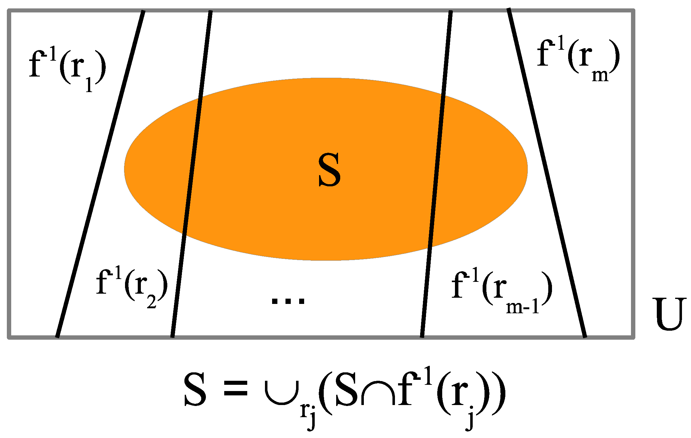
A (real-valued) numerical attribute (or observable) on $U=\left\{u_1,\dots ,u_n\right\}$ is a function $f:U\to \mathbb{R}$ from U to the real numbers. It assigns a real number to each element of U. If it takes only the values of 0 and 1, then it is an attribute and is represented in the special notation as a characteristic function ${\chi }_S:U\to 2=\left\{0,1\right\}$ where $S=\left\{u_i\in U|{\chi }_S\left(u_i\right)=1\right\}={\chi }_S^{-1}\left(1\right)$, the set of elements taking on the value of 1. The set of real numbers that have an element of U mapped to them by f is the image or spectrum of f, denoted $f\left(U\right)\subseteq \mathbb{R}$. Each number $r\in f\left(U\right)$ in the spectrum of f is a definite-value or eigenvalue of f. The inverse image subset $f^{-1}\left(r\right)\subseteq U$ of U is the set of elements of U mapped to an eigenvalue r, i.e., $f^{-1}\left(r\right)=\left\{u_i\in U|f\left(u_i\right)=r\right\}$. That inverse image generates a subspace $\wp \left(f^{-1}\left(r\right)\right)\subseteq \wp \left(U\right)$ called the eigenspace associated with the eigenvaluer. Thus, if $f:\left\{a,b,c\right\}\to \mathbb{R}$ had $f\left(a\right)=f\left(b\right)=3$ and $f\left(c\right)=-5$, then $f^{-1}\left(3\right)=\left\{a,b\right\}$ and $\wp \left(f^{-1}\left(3\right)\right)=\left\{\varnothing ,\left\{a\right\},\left\{b\right\},\left\{a,b\right\}\right\}$ is the eigenspace associated with the eigenvalue of 3. The non-zero vectors in the eigenspace for r are also called definite-states or eigenstates of f. All the non-empty subsets in $\wp \left(f^{-1}\left(r\right)\right)$ are constant sets of f, i.e., subsets of U on which f has the same value of r.

A partition $\pi$ on U is a set of non-empty subsets $\pi =\left\{B_1,\dots ,B_m\right\}$, called the blocks of $\pi$, such that the blocks are disjoint, i.e., $B_j\cap B_k=\varnothing$ for $j\ne k$, and their union is all of U, i.e., ${\cup }_{j=1}^m{B}_j=U$. Each numerical attribute $f:U\to \mathbb{R}$ determines a partition $f^{-1}=\left\{f^{-1}\left(r\right)|r\in f\left(U\right)\right\}$ on U called the inverse-image of f. Each block $f^{-1}\left(r\right)$ of the partition $f^{-1}$ generates an eigenspace $\wp \left(f^{-1}\left(r\right)\right)$. The set of eigenspaces of f, ${\left\{\wp \left(f^{-1}\left(r\right)\right)\right\}}_{r\in f\left(U\right)}$ form a direct-sum decomposition (DSD) of $\wp \left(U\right)$ in the sense that every non-zero vector (i.e., every non-empty subset of U) can be uniquely represented as the sum of non-zero vectors from the subspaces in the DSD. For instance, in the example $f:\left\{a,b,c\right\}\to \mathbb{R}$, the vector or subset $\left\{a,c\right\}$ is the sum of $\left\{a\right\}\in \wp \left(f^{-1}\left(3\right)\right)$ and $\left\{c\right\}\in \wp \left(f^{-1}\left(-5\right)\right)$. A DSD of a vector space is the vector space version of a partition on a set.

In QM, every observable or Hermitian operator F has a set of eigenspaces $V_{\lambda }$ that form a direct-sum decomposition of the Hilbert space V. In QM/Sets, the eigenspace for an eigenvalue r of a numerical attribute $f:U\to \mathbb{R}$ is $\wp \left(f^{-1}\left(r\right)\right)$, which also form a DSD of $\wp \left(U\right)$. In QM, different eigenspaces $V_{\lambda }$ and $V_{{\lambda }^{\prime }}$ for $\lambda \ne {\lambda }^{\prime }$ are ‘disjoint’ is the sense that their intersection is the zero space. Similarly, for eigenvalues $r\ne r^{\prime }$, the intersection of $\wp \left(f^{-1}\left(r\right)\right)$ and $\wp \left(f^{-1}\left(r^{\prime }\right)\right)$ is only the empty set subspace $\left\{\varnothing \right\}$. In QM, the projections $P_{\lambda }:V\to V$ to the eigenspaces $V_{\lambda }$ are complete in the sense that the sum of the projections is the identity operator: ${\sum }_{\lambda }{P}_{\lambda }=I:V\to V$. In QM/Sets, the corresponding projections are: $f^{-1}\left(r\right)\cap \left(\right):\wp \left(U\right)\to \wp \left(U\right)$ and the union of the images on any $S\in \wp \left(U\right)$ is: ${\cup }_{r\in f\left(U\right)}\left(f^{-1}\left(r\right)\cap S\right)=S$ as illustrated in Figure 1.

Figure 1. Subset S expressed as union over $r\in f\left(U\right)$ of disjoint intersections $f^{-1}\left(r\right)\cap S$.

Since the sets in the union are disjoint, the union translates into a sum in the vector space $\wp \left(U\right)$ [where the sum is $S+T=S\cup T-\left(S\cap T\right)$], so we have: ${\sum }_{r\in f\left(U\right)}{f}^{-1}\left(r\right)\cap \left(\right)=I:\wp \left(U\right)\to \wp \left(U\right)$.

To approach the probability calculus for numerical attributes $f:U\to \mathbb{R}$, the QM equation: ${∥\psi ∥}^2=⟨\psi |\psi ⟩={\sum }_{\lambda }{∥P_{\lambda }\left(\psi \right)∥}^2$ is expressed in QM/Sets as: ${∥S∥}_U^2=⟨{S|}_{U}S⟩={\sum }_{r\in f\left(U\right)}{∥f^{-1}\left(r\right)\cap S∥}_U^2={\sum }_{r\in f\left(U\right)}\left|f^{-1}\left(r\right)\cap S\right|=\left|S\right|$. Then we normalize to have probabilities that sum to one: ${\sum }_{\lambda }\frac{{∥P_{\lambda }\left(\psi \right)∥}^2}{{∥\psi ∥}^2}=1$ for $\psi \ne 0$ in QM, and ${\sum }_{r\in f\left(U\right)}\frac{{∥f^{-1}\left(r\right)\cap S∥}_U^2}{{∥S∥}_U^2}={\sum }_r\frac{\left|f^{-1}\left(r\right)\cap S\right|}{\left|S\right|}=1$ for $S\ne \varnothing$ in QM/Sets. Then, when measuring $\psi$ by the observable F, the probability of getting the eigenvalue $\lambda$ is:

$$\mathrm{Pr}\left(\lambda |\psi \right)=\frac{{∥P_{\lambda }\left(\psi \right)∥}^2}{{∥\psi ∥}^2}$$

and the corresponding probability for getting the eigenvalue r of the numerical attribute f when conditioned by S is:

$$\mathrm{Pr}\left(r|S\right)=\frac{{∥f^{-1}\left(r\right)\cap S∥}_U^2}{{∥S∥}_U^2}=\frac{\left|f^{-1}\left(r\right)\cap S\right|}{\left|S\right|}.$$

These probabilities are for equiprobable outcomes; the machinery for the general case is developed below.

Table 2 starts building the connections or translation dictionary between the pedagogical model of QM/Sets and QM (where ${\left\{\left|u_i\right.⟩\right\}}_{i=1}^n$ is an orthonormal (ON) basis for V and ${\alpha }_i^{*}$ is the complex conjugate of ${\alpha }_i$).

Table 2. Initial connections between QM/Sets and QM.

QM/Sets	QM
$⟨\left\{u_i\right\}|S⟩={\chi }_S\left(u_i\right)$	$\left|\psi \right.⟩={\sum }_i{\alpha }_i\left|u_i\right.⟩$; $⟨u_i|\psi ⟩={\alpha }_i$
${\sum }_{i=1}^n$$\left|\left\{u_i\right\}\right.⟩{\left.⟨\left\{u_i\right\}\right|}_{U}S⟩={\sum }_{i=1}^n{\chi }_S\left(u_i\right)\left|\left\{u_i\right\}\right.⟩=\left|S\right.⟩$	${\sum }_{i=1}^n\left|u_i\right.⟩⟨\left.u_i\right|\psi ⟩=\left|\psi \right.⟩$
$⟨{T|}_{U}S⟩={\sum }_{i=1}^n{\chi }_T\left(u_i\right){\chi }_S\left(u_i\right)=\left|T\cap S\right|$	$⟨\psi |{\psi }^{\prime }⟩={\sum }_{i=1}^n{\alpha }_i^{*}{\alpha }_i^{\prime }$
${∥S∥}_U=\sqrt{⟨{S|}_{U}S⟩}=\sqrt{\left|S\right|}$	$∥\psi ∥=\sqrt{⟨\psi |\psi ⟩}$
$\mathrm{Pr}\left(u_i|S\right)=\frac{{∥⟨u_i{|}_{U}S⟩∥}^2}{{∥⟨{S|}_{U}S⟩∥}^2}=\frac{\left|\left\{u_i\right\}\cap S\right|}{\left|S\right|}$	$\mathrm{Pr}\left(v_i|\psi \right)=\frac{{∥⟨v_i|\psi ⟩∥}^2}{{∥⟨\psi |\psi ⟩∥}^2}$
Numerical attribute $f:U\to \mathbb{R}$	Hermitian $F:V\to V$
$r\ne r^{\prime }$; $\wp \left(f^{-1}\left(r\right)\right)\cap \wp \left(f^{-1}\left(r^{\prime }\right)\right)=\left\{\varnothing \right\}$	$\lambda \ne {\lambda }^{\prime }$; $V_{\lambda }\cap V_{{\lambda }^{\prime }}=\left\{0\right\}$
${\sum }_{r\in f\left(U\right)}{f}^{-1}\left(r\right)\cap \left(\right)=I:\wp \left(U\right)\to \wp \left(U\right)$	${\sum }_{\lambda }{P}_{V_{\lambda }}=I:V\to V$
${\sum }_{r\in f\left(U\right)}\frac{{∥f^{-1}\left(r\right)\cap S∥}_U^2}{{∥S∥}_U^2}={\sum }_r\frac{\left|f^{-1}\left(r\right)\cap S\right|}{\left|S\right|}=1$	${\sum }_{\lambda }\frac{{∥P_{\lambda }\left(\psi \right)∥}^2}{{∥\psi ∥}^2}=1$
$\mathrm{Pr}\left(r|S\right)=\frac{{∥f^{-1}\left(r\right)\cap S∥}_U^2}{{∥S∥}_U^2}=\frac{\left|f^{-1}\left(r\right)\cap S\right|}{\left|S\right|}$	$\mathrm{Pr}\left(\lambda |\psi \right)=\frac{{∥P_{\lambda }\left(\psi \right)∥}^2}{{∥\psi ∥}^2}$

3.2. The Yoga of Linearization

We have been implicitly using a bit of mathematical folklore that we will call the Yoga of Linearization. It connects set concepts with the corresponding vector space concepts. The idea is to first look at U as just a set to which a set concept may be applied (e.g., the notion of subset, numerical attribute, or partition on a set). Then take U to be a basis set of a vector space V (over a given field $\mathbb{k}$) and the corresponding vector space notion is the notion generated by the set concept applied to the basis set. For instance, the notion of a subset S of a basis set generates the notion of a subspace $\left[S\right]$ generated by S, so the Yoga connects the notion of a subset $S\subseteq U$ and the notion of a subspace $\left[S\right]\subseteq V$. If we apply a set partition to a basis set U, then each block in the partition of U generates a subspace, and the set of subspaces generated by the blocks of the partition form a direct-sum decomposition of the vector space, so the Yoga connects the set notion of a partition to the vector space notion of a DSD. A numerical attribute on a set $f:U\to \mathbb{R}$ defines a linear operator $F:V\to V$ (assuming V is a vector space over a field containing the reals), which on the basis set U is given by $F{u}_i=f\left(u_i\right)u_i$ where the $u_i\in U$ are basis vectors and the definition of a linear operator on a basis set extends linearly to the whole space. Thus, the Yoga connects a real-valued numerical attribute with a linear operator on a vector space over a field containing the reals, e.g., the complex numbers, where the operator has real eigenvalues $r\in f\left(U\right)$.

If the vector space such as $V={\mathbb{Z}}_2^n$ is over a field ${\mathbb{Z}}_2$ not containing the reals, then the inverse image partition $f^{-1}={\left\{f^{-1}\left(r\right)\right\}}_{r\in f\left(U\right)}$ defines a DSD in the vector space, which may have many of the main properties of a linear operator (see next section). For a numerical attribute $f:U\to \mathbb{R}$, let “$f\upharpoonright S=rS$” stand for the statement that f restricted to a subset S has the constant value r on that subset. The Yoga connects that equation to the eigenvalue/eigenvector equation $F{u}_i=r{u}_i$. Then constant sets of a numerical attribute $f:U\to \mathbb{R}$ corresponds to eigenvectors of the linear operator $F:V\to V$ defined on the basis set U by $F{u}_i=f\left(u_i\right)u_i$ and the constant value r on a constant set corresponds to the eigenvalue of the eigenvector. When the numerical attribute is a characteristic function ${\chi }_S:U\to \left\{0,1\right\}$, then the corresponding linear operator defined by $P_{\left[S\right]}{u}_i={\chi }_S\left(u_i\right)u_i$ is the projection operator $P_{\left[S\right]}$ onto the subspace $\left[S\right]$ generated by $S={\chi }_S^{-1}\left(1\right)\subseteq U$. In the general case of $f:U\to \mathbb{R}$ defining $F:V\to V$, there is a ‘spectral decomposition’ of f in terms of the characteristic functions for ${\left\{f^{-1}\left(r\right)\right\}}_{r\in f\left(U\right)}$, i.e., $f={\sum }_{r\in f\left(U\right)}r{\chi }_{f^{-1}\left(r\right)}$, that corresponds to the usual spectral decomposition of the linear operator F as $F={\sum }_{r\in f\left(U\right)}r{P}_{\left[f^{-1}\left(r\right)\right]}$.

In this manner, the Yoga builds up a translation dictionary of set concepts and the corresponding vector space concepts, as in Table 3.

Table 3. Set concepts and corresponding vector space concepts.

Set Concepts of QM/Sets	Vector-Space Concepts of QM
Subset $S\subseteq U$	Subspace $\left[S\right]\subseteq V$
Cardinality $\left|S\right|$ of S	Dimension of $\left[S\right]$
Numerical attribute $f:U\to \mathbb{R}$	Obs. $F:V\to V$ defined $F{u}_i=f\left(u_i\right)u_i$
Direct sum $U={\uplus }_{r\in f\left(U\right)}{f}^{-1}\left(r\right)$	Direct sum $V={\oplus }_{r\in f\left(U\right)}\left[f^{-1}\left(r\right)\right]$
Partition ${\left\{f^{-1}\left(r\right)\right\}}_{r\in f\left(U\right)}$	DSD ${\left\{\left[f^{-1}\left(r\right)\right]\right\}}_{r\in f\left(U\right)}$
$f\upharpoonright S=rS$	$F{u}_i=r{u}_i$
Constant set S of f	Eigenvector $u_i$ of F
Value r on constant set S	Eigenvalue r of eigenvector $u_i$
Set of r-constant sets $\wp \left(f^{-1}\left(r\right)\right)$	Eigenspace $V_r=\left[f^{-1}\left(r\right)\right]$ of r-eigenvectors
Characteristic fcn. ${\chi }_S:U\to \left\{0,1\right\}$	Projection operator $P_{\left[S\right]}u={\chi }_S\left(u\right)u$
Spectral Decomp. $f={\sum }_{r\in f\left(U\right)}r{\chi }_{f^{-1}\left(r\right)}$	Spectral Decomp. $F={\sum }_{r\in f\left(U\right)}r{P}_{\left[f^{-1}\left(r\right)\right]}$

Our simplified model of QM is based on set notions and, where possible, the set notions connected by the Yoga to the vector spaces $\wp \left(U\right)$ over ${\mathbb{Z}}_2$. When the vector space V is a finite-dimensional Hilbert vector space over $\mathbb{C}$, then the Yoga shows how the machinery in the simplified model corresponds to the full-blown mathematical machinery of QM [1]. But when $V={\mathbb{Z}}_2^n$, then only a characteristic function ${\chi }_S:U\to \left\{0,1\right\}$ defines a linear operator $P_{\left[S\right]}:{\mathbb{Z}}_2^n\to {\mathbb{Z}}_2^n$, but a general numerical attribute $f:U\to \mathbb{R}$ still defines a partition $f^{-1}$ on U and the DSD ${\left\{\wp \left(f^{-1}\left(r\right)\right)\right\}}_{r\in f\left(U\right)}$ of ${\mathbb{Z}}_2^n$. The same holds for any other basis set for ${\mathbb{Z}}_2^n$. For instance, for the $U^{\prime }$-basis of Table 1, the numerical attribute $g:U^{\prime }\to \mathbb{R}$ given by $g\left(a^{\prime }\right)=g\left(c^{\prime }\right)=1$ and $g\left(b^{\prime }\right)=2$, induces the partition $\left\{\left\{a^{\prime },c^{\prime }\right\},\left\{b^{\prime }\right\}\right\}$ on $U^{\prime }$, and the DSD:

$$\left\{\left\{\varnothing ,\left\{a^{\prime }\right\},\left\{c^{\prime }\right\},\left\{a^{\prime },c^{\prime }\right\}\right\},\left\{\varnothing ,\left\{b^{\prime }\right\}\right\}\right\}=\left\{\left\{\varnothing ,\left\{a,b\right\},\left\{b,c\right\},\left\{a,c\right\}\right\},\left\{\varnothing ,\left\{a,b,c\right\}\right\}\right\}$$

where the DSD expressed in terms of the U-basis is not generated by a partition on U.

As we will see in the next section, for many purposes, the important notion for an observable is not the Hermitian linear operator itself but its DSD of eigenspaces.

3.3. Commutativity and Conjugacy of Observables

In full-blown QM, the observables are represented by Hermitian linear operators $F:V\to V$ on a Hilbert space over the complex numbers $\mathbb{C}$. One of the features of QM in contrast with classical mechanics is that these operators for different observables might commute, not commute, or even be conjugate like position and momentum. A linear operator is determined by its definition on a basis set; each basis vector is assigned a number in the base field, and in the case of Hermitian operators, those assigned values are always real numbers $\mathbb{R}\subseteq \mathbb{C}$. But in our pedagogical model QM/Sets, the only linear operators $\widehat{S}:\wp \left(U\right)\to \wp \left(U\right)$ are those that assign an element of the field ${\mathbb{Z}}_2=\left\{0,1\right\}$ to the elements of U, i.e., the characteristic functions ${\chi }_S:U\to {\mathbb{Z}}_2=\left\{0,1\right\}$.

Hence, the question arises: how can we represent commutativity, non-commutativity, and conjugacy in QM/Sets for numerical attributes $f:U\to \mathbb{R}$? The answer is that each Hermitian operator $F:V\to V$ in QM determines the DSD of its eigenspaces, and the commutativity properties depend solely on the DSDs.

The first step in working this out is to notice that the notion of a subspace or a DSD of subspaces is basis-independent. In the previous example of $f:U\to \mathbb{R}$, we had the eigenspace $\wp \left(f^{-1}\left(3\right)\right)=\left\{\varnothing ,\left\{a\right\},\left\{b\right\},\left\{a,b\right\}\right\}$. But that subspace can be equally well expressed in the $U^{\prime }$-basis as $\left\{\varnothing ,\left\{b^{\prime },c^{\prime }\right\},\left\{a^{\prime },b^{\prime },c^{\prime }\right\},\left\{a^{\prime }\right\}\right\}$. Since a DSD is a certain type of collection of subspaces, it is also a basis-independent notion–even though it may be first defined using some particular basis. The point is that the commutativity properties can be defined in QM and in QM/Sets solely in terms of the DSDs of eigenspaces.

Suppose we have two different basis sets, U and $U^{\prime }$ for ${\mathbb{Z}}_2^n$ and two numerical attributes, $f:U\to \mathbb{R}$ and $g:U^{\prime }\to \mathbb{R}$, which then define two DSDs ${\left\{\wp \left(f^{-1}\left(r\right)\right)\right\}}_{r\in f\left(U\right)}$ and ${\left\{\wp \left(g^{-1}\left(s\right)\right)\right\}}_{s\in g\left(U^{\prime }\right)}$. For two partitions $\pi =\left\{B_1,\dots ,B_m\right\}$ and $\sigma =\left\{C_1,\dots ,C_{m^{\prime }}\right\}$ on the same set U, their join $\pi \vee \sigma$ is the partition whose blocks are the non-empty intersections $B_j\cap C_{j^{\prime }}$ of blocks from $\pi$ and $\sigma$. Since DSDs can be seen as the vector space versions of partitions, we would like to perform a join-like operation on two DSDs. Since a subspace can be represented on any basis, we need to represent the subspaces of two DSDs on the same basis before we can determine the intersection of the subspaces that serve as the blocks in the vector space partitions. Hence, instead of ${\left\{\wp \left(f^{-1}\left(r\right)\right)\right\}}_{r\in f\left(U\right)}$ and ${\left\{\wp \left(g^{-1}\left(s\right)\right)\right\}}_{s\in g\left(U^{\prime }\right)}$, we abstractly consider two DSDs ${\left\{W_j\right\}}_{j=1}^m$ and ${\left\{V_{j^{\prime }}\right\}}_{j^{\prime }=1}^{m^{\prime }}$ (which could be the DSDs of eigenspaces of two observables in QM), and then perform a join-like operation to get the set $\left\{W_j\cap V_{j^{\prime }}|W_j\cap V_{j^{\prime }}\ne \left\{0\right\};j=1,\dots ,m^{\prime };j^{\prime }=1,\dots ,m^{\prime }\right\}$ of non-zero subspaces (using the fact that the intersection of subspaces is a subspace). In terms of the original numerical attributes $f:U\to \mathbb{R}$ and $g:U^{\prime }\to \mathbb{R}$, the non-zero vectors in an intersection $W_j\cap V_{j^{\prime }}$, e.g., in an intersection $\wp \left(f^{-1}\left(r\right)\right)\cap \wp \left(g^{-1}\left(s\right)\right)$ (with subsets represented in the same basis), are eigenvectors (or constant sets) of both f and g, which are called “simultaneous eigenvectors” in QM. Then we take the sums of all those simultaneous eigenvectors to generate a subspace $\mathcal{SE}$ of the space ${\mathbb{Z}}_2^n$. The commutativity properties of the observables in QM and the numerical attributes in QM/Sets can then be defined solely in terms of the DSDs of eigenspaces in both cases:

$$\begin{array}{c}{\left\{W_j\right\}}_{j=1}^m\mathrm{and}{\left\{V_{j^{\prime }}\right\}}_{j^{\prime }=1}^{m^{\prime }}commute\mathrm{if}\mathcal{SE}\mathrm{is}\mathrm{the}\mathrm{whole}\mathrm{space}\\ (V\mathrm{in}\mathrm{QM}\mathrm{or}{\mathbb{Z}}_2^n\mathrm{in}\mathrm{QM}/\mathrm{Sets}),\mathrm{and}\\ {\left\{W_j\right\}}_{j=1}^m\mathrm{and}{\left\{V_{j^{\prime }}\right\}}_{j^{\prime }=1}^{m^{\prime }}\mathrm{are}conjugate\mathrm{if}\mathcal{SE}\mathrm{is}\mathrm{the}\mathrm{zero}\mathrm{space}\\ (\mathrm{in}\mathrm{QM}\left\{0\right\}\mathrm{and}\mathrm{in}\mathrm{QM}/\mathrm{Sets}\left\{\varnothing \right\}).\end{array}$$

The join-like operation of taking all the non-zero subspaces $W_j\cap V_{j^{\prime }}$ only creates another DSD in the commutative case when $\mathcal{SE}=V$ or ${\mathbb{Z}}_2^n$, and it is only then that the operation is properly called the join of DSDs. As Hermann Weyl put it when referring to the vector space partitions or DSDs as “gratings”, the “combination of two gratings presupposes commutability….” [8] (p. 257).

Commutativity example: Any two numerical attributes defined on the same basis set will commute, but that is not necessary. Let $f:\left\{a,b,c\right\}\to \mathbb{R}$ have $f\left(a\right)=1$ and $f\left(b\right)=f\left(c\right)=0$. On the $U^{*}$-basis of Table 1, let $g:U^{*}\to \mathbb{R}$ be defined by $g\left(a^{*}\right)=2$, $g\left(b^{*}\right)=3$, and $g\left(c^{*}\right)=4$. Then the DSD defined by f is $\left\{\wp \left(f^{-1}\left(1\right)\right),\wp \left(f^{-1}\left(0\right)\right)\right\}=\left\{\left\{\varnothing ,\left\{a\right\}\right\},\left\{\varnothing ,\left\{b\right\},\left\{c\right\},\left\{b,c\right\}\right\}\right\}$, and the DSD defined by g is $\left\{\wp \left(g^{-1}\left(2\right)\right),\wp \left(g^{-1}\left(3\right)\right),\right.$$\left.\wp \left(g^{-1}(4\right)\right\}=\left\{\left\{\varnothing ,\left\{a^{*}\right\}\right\},\left\{\varnothing ,\left\{b^{*}\right\}\right\},\left\{\varnothing ,\left\{c^{*}\right\}\right\}\right\}$. To consider the intersections of the subspaces in the DSDs, we need to express them both on the same basis. Taking the U-basis as the ‘computational basis’, we have the two DSDs as:

$$\begin{array}{c}\left\{\left\{\varnothing ,\left\{a\right\}\right\},\left\{\varnothing ,\left\{b\right\},\left\{c\right\},\left\{b,c\right\}\right\}\right\}\mathrm{for}f,\\ \mathrm{and}\\ \left\{\left\{\varnothing ,\left\{a\right\}\right\},\left\{\varnothing ,\left\{b\right\}\right\},\left\{\varnothing ,\left\{b,c\right\}\right\}\right\}\mathrm{for}g.\end{array}$$

Then taking all the possible intersections between the subspaces in the two DSDs, we see that the simultaneous eigenvectors are $\left\{a\right\}$, $\left\{b\right\}$, and $\left\{b,c\right\}$. These simultaneous eigenvectors form a basis, so they generate by their sums all the vectors or subsets in the whole space $\wp \left(U\right)$ so that those two DSDs commute.

Conjugacy example: Take $f:U\to \mathbb{R}$ as $f\left(a\right)=1$, $f\left(b\right)=2$, and $f\left(c\right)=3$, and take $g:U^{\prime }\to \mathbb{R}$ as $g\left(a^{\prime }\right)=4$, $g\left(b^{\prime }\right)=5$, and $g\left(c^{\prime }\right)=6$ ($U^{\prime }$ is as in Table 1). Then the DSD determined by f is $\left\{\left\{\varnothing ,\left\{a\right\}\right\},\left\{\varnothing ,\left\{b\right\}\right\},\left\{\varnothing ,\left\{c\right\}\right\}\right\}$, and the DSD determined by g is in the $U^{\prime }$-basis, $\left\{\left\{\varnothing ,\left\{a^{\prime }\right\}\right\},\left\{\varnothing ,\left\{b^{\prime }\right\}\right\},\left\{\varnothing ,\left\{c^{\prime }\right\}\right\}\right\}$ which translated into the U-basis, gives the following two DSDs:

$$\begin{array}{c}\left\{\left\{\varnothing ,\left\{a\right\}\right\},\left\{\varnothing ,\left\{b\right\}\right\},\left\{\varnothing ,\left\{c\right\}\right\}\right\}\mathrm{for}f,\\ \mathrm{and}\\ \left\{\left\{\varnothing ,\left\{a,b\right\}\right\},\left\{\varnothing ,\left\{a,b,c\right\}\right\},\left\{\varnothing ,\left\{b,c\right\}\right\}\right\}\mathrm{for}g.\end{array}$$

In this case, there are no simultaneous eigenvectors, so $\mathcal{SE}=\left\{\varnothing \right\}$, and thus those two DSDs are conjugate. Recalling that being a definite state (i.e., an eigenstate) or an indefinite state (i.e., a superposition state) depends on the basis, the key feature that determined conjugacy in this case is that all the definite states or eigenstates in one basis were indefinite states or superpositions in the other basis (see Table 1) and both numerical attributes were assigned different numbers to different eigenstates. Hence, like the conjugate observables of position and momentum in QM, there is no non-zero vector that is a definite state or eigenstate of both numerical attributes. If any vector or state is an eigenstate or definite state of one numerical attribute, then it has to be a superposition or indefinite state for the other numerical attribute.

Since in all cases, the DSDs are determined by the numerical attributes, we may also say that those numerical attributes are commutative or conjugate as the case may be.

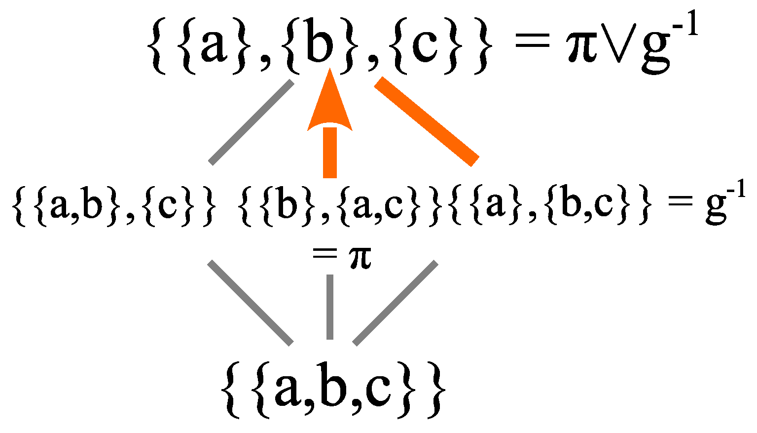
The join of the two inverse-image partitions $f^{-1}$ and $g^{-1}$ always exist if they are compatible in the sense of being defined on the same universe set. That is the QM/Sets version of commuting observables in QM. The QM/Set version of Dirac’s complete set of commuting observables (CSCO) [9] is easily constructed.

QM/Sets: Let $f,g,\dots ,h:U\to \mathbb{R}$ be numerical attributes on U. They are said to be a complete Set of compatible attributes (CSCA) if the join of their (inverse-image) partitions is a partition with all subsets of cardinality one. Then each element $u_i\in U$ can be uniquely characterized by the ordered set of values $f\left(u_i\right),g\left(u_i\right),\dots ,h\left(u_i\right)$.

QM: Let $F,G,\dots ,H:V\to V$ be commuting observables on V. They are said to be a complete set of commuting observables (CSCO) if the join of their vector space partitions (DSDs) is a DSD with all subspaces of dimension one. Then each simultaneous eigenvector can be uniquely characterized by the ordered set of their eigenvalues. If $U=\left\{u_1,\dots ,u_n\right\}$ is a basis of simultaneous eigenvectors and $f:U\to \mathbb{R}$, $g:U\to \mathbb{R}$,…, $h:U\to \mathbb{R}$ are the eigenvalue functions assigning the eigenvalues to the simultaneous eigenvectors of the observables $F,G,\dots ,H$ respectively, then the ordered set of eigenvalues that characterize the eigenvectors $u_i\in U$ is $f\left(u_i\right),g\left(u_i\right),\dots ,h\left(u_i\right)$.

This is a paradigm example of a translation or correlation dictionary between QM/Sets and full QM.

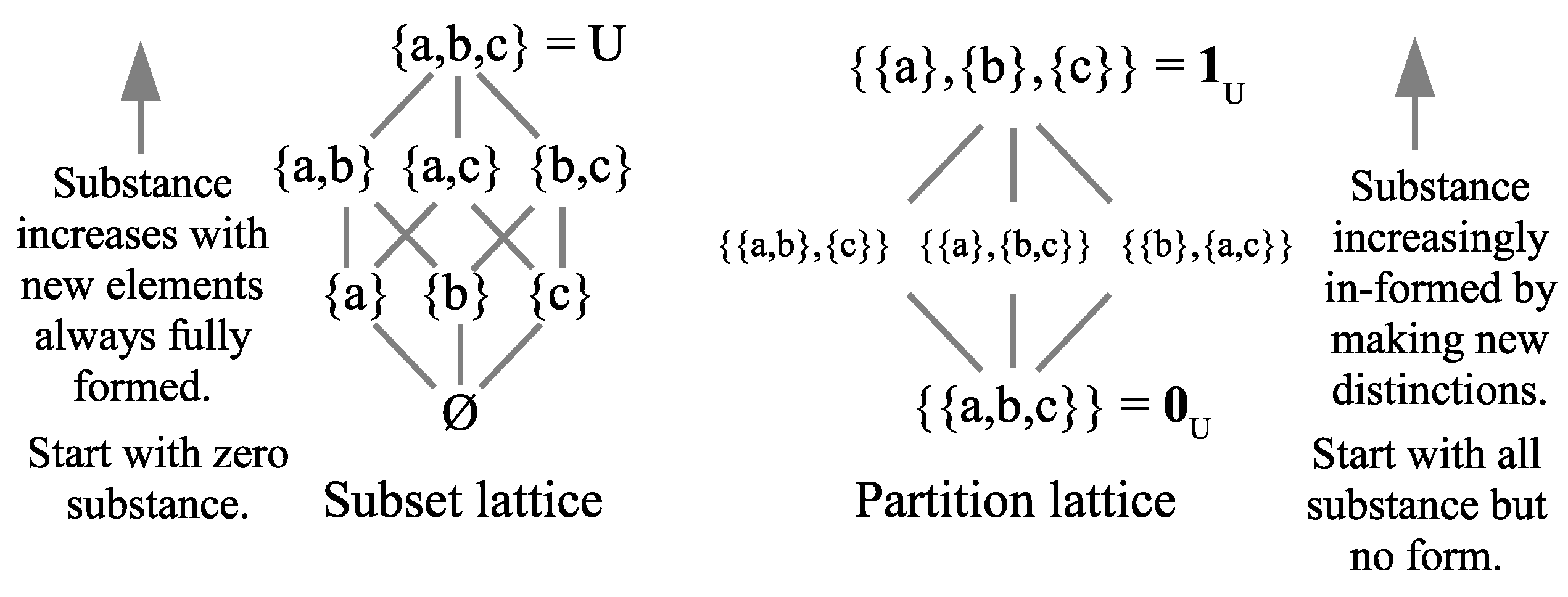
3.4. The Lattice of Partitions

Given a set U ($\left|U\right|\ge 2$), recall that a partition $\pi$ on $U=\left\{u_1,\dots ,u_n\right\}$ is a set of non-empty subsets $\pi =\left\{B_1,\dots ,B_m\right\}$ that are pairwise disjoint and jointly exhaustive of U. It is interesting to note that a partition can be given a DSD-type definition as a set of non-empty subsets $\pi =\left\{B_1,\dots ,B_m\right\}$ so that any non-empty subset $S\subseteq U$ can be uniquely represented as the union of subsets of the blocks $B_1,\dots ,B_m$. If the blocks were not disjoint, say $S=B_j\cap B_k\ne \varnothing$, then that non-empty subset S would have two representations as a subset of the blocks, so uniqueness fails. And if the blocks were not jointly exhaustive, then the non-empty subset $S=U-{\cup }_{j=1}^m{B}_j$ would have no representation as a union of subsets of the blocks. The unique representation of S is given by the union of the projection operators $B_j\cap \left(\right):\wp \left(U\right)\to \wp \left(U\right)$, i.e., ${\cup }_{j=1}^m\left(B_j\cap S\right)=S$. Thus, a set partition is the set version of a vector space DSD. Moreover, when sets are treated as vectors in $\wp \left(U\right)$, then ${\left\{\wp \left(B_j\right)\right\}}_{j=1}^m$ is a DSD of the vector space $\wp \left(U\right)$ if $\left\{B_1,\dots ,B_m\right\}$ is a partition of U.

An indistinction or indit of $\pi$ is an ordered pair of elements $\left(u_i,u_k\right)$ that in the same block of $\pi$. The set of all indits is the indit set $\mathrm{indit}\left(\pi \right)={\cup }_{j=1}^m\left(B_j\times B_j\right)\subseteq U\times U$, which is the equivalence relation associated with the partition $\pi$. A distinction or dit of $\pi$ is an ordered pair of elements $\left(u_i,u_k\right)$ in different blocks of $\pi$, so the set of all dits, the ditset $\mathrm{dit}\left(\pi \right)$, is just the complement of the equivalence relation $\mathrm{indit}\left(\pi \right)$ in $U\times U$.

Let $\Pi \left(U\right)$ be the set of all partitions on U. There is a partial order on $\Pi \left(U\right)$ given by the inclusion of ditsets. That is, for partitions $\pi =\left\{B_1,\dots ,B_m\right\}$ and $\sigma =\left\{C_1,\dots ,C_{m^{\prime }}\right\}$, the partial order is: $\sigma \precsim \pi$ if $\mathrm{dit}\left(\sigma \right)\subseteq \mathrm{dit}\left(\pi \right)$. This is also the equivalent refinement partial ordering where $\pi$ refines $\sigma$ if for every block $B_j\in \pi$, there is a block $C_{j^{\prime }}\in \sigma$ such that $B_j\subseteq C_{j^{\prime }}$. In the partial order on $\Pi \left(U\right)$, there is a maximum or top partition, which is the discrete partition ${\mathbf{1}}_U={\left\{\left\{u_i\right\}\right\}}_{i=1}^n$ where all the blocks are the singletons of the elements $u_i\in U$. And there is a minimum or bottom partition which is the indiscrete partition, ${\mathbf{0}}_U=\left\{U\right\}$ where there is only one block, which is all of U.

For $\pi ,\sigma \in \Pi \left(U\right)$, join operation gives the least upper bound on $\pi$ and $\sigma$ in the refinement ordering. There is also a meet or greatest lower bound of two partitions $\pi$ and $\sigma$. When two blocks $B_j\in \pi$ and $C_{j^{\prime }}\in \sigma$ have a non-empty intersection, they ‘blob’ together like two touching drops of water. Eventually, blobs will form of blocks from both partitions until they intersect no other blocks of the other partition. Those minimal unions of $\pi$-blocks and $\sigma$-blocks are the blocks of the meet $\pi \wedge \sigma$. The meet could also be defined as the partition formed from the equivalence relation that is the intersection of all equivalence relations containing the indit sets of $\pi$ and $\sigma$. The indiscrete partition ${\mathbf{0}}_U$ is nicknamed “The Blob” since like in the Hollywood movie of the same name, it absorbs everything it meets: ${\mathbf{0}}_U\wedge \pi ={\mathbf{0}}_U$.

The join and meet operations on partitions were known in the nineteenth century (e.g., Richard Dedekind and Ernst Schröder) and they turn $\Pi \left(U\right)$ into a lattice (a partial order with joins and meets). The lattice of partitions on $U=\left\{a,b,c\right\}$ is given in Figure 2. The lines between partitions indicate refinement with no partitions in between.

Figure 2. Lattice of partitions on $U=\left\{a,b,c\right\}$.

3.5. Superposition Subsets and Density Matrices

Given a basis U for a vector space V, any vector has the form of a linear combination of the basis vectors ${\sum }_{i=1}^n{\alpha }_i{u}_i$ where the ${\alpha }_i$ are scalars from the field, e.g., $\mathbb{C}$ in QM and ${\mathbb{Z}}_2$ in QM/Sets. The support of the vector is the set of basis vectors with non-zero coefficients ${\alpha }_i$. We can think of taking the support of a vector as ‘skeletionizing’ it to yield a set $S\subseteq U$ of basis vectors. If the support is a singleton, then the vector is a definite state or an eigenstate (perhaps not normalized), and if the support is a multiple-element subset of U, then the vector is a superposition or indefinite state. Hence, we need to mathematically distinguish between two types of subsets of U, the ordinary ‘discrete subsets’ $S\subseteq U$ where the elements are perfectly distinct from one another, and the ‘superposition subsets’, denoted $\Sigma S$, where the elements are blobbed or blurred together in an indefinite state, which represents the support of a superposition state in QM. An event in classical finite probability theory is a subset of the outcome space U. Then superposition subsets can be viewed as an extension of probability theory to include superposition events in addition to the usual discrete events where the outcomes are all distinct, i.e., not blobbed or blurred together.

One way to mathematically distinguish between these two types of subsets or events is to move from representing subsets as one-dimensional vectors to using two-dimensional matrices. We start by using incidence matrices of binary relations. A subset $R\subseteq U\times U$ is a binary relation on U, and it can be represented by the $n\times n$ incidence matrix $\mathrm{In}\left(R\right)$, where each entry in the matrix is $\mathrm{In}{\left(R\right)}_{ij}=1$ if $\left(u_i,u_j\right)\in R$ and otherwise 0. Then for each subset $S\subseteq U$, we use the diagonal $\Delta S=\left\{\left(u_i,u_i\right)|u_i\in S\right\}$ as the binary relation to represent the discrete subset S; we use the Cartesian product $S\times S$ as the binary relation to represent the superposition subset $\Sigma S$. Then for $U=\left\{a,b,c\right\}$, the subset $S=\left\{a,c\right\}$ gives the two incidence matrices:

$$\mathrm{In}\left(\Delta S\right)=\left[\begin{array}{ccc}1& 0& 0\\ 0& 0& 0\\ 0& 0& 1\end{array}\right]\mathrm{and}\mathrm{In}\left(S\times S\right)=\left[\begin{array}{ccc}1& 0& 1\\ 0& 0& 0\\ 1& 0& 1\end{array}\right].$$

The matrix $\mathrm{In}\left(\Delta S\right)$ is always a diagonal matrix and represents the discrete event $S\subseteq U$, and $\mathrm{In}\left(S\times S\right)$ has the same diagonal but also has non-zero off-diagonal elements to indicate which elements of U are blobbed, blurred, or cohered together in the superposition subset $\Sigma S$. In the case of a singleton $S=\left\{u_i\right\}$, then the superposition set is the same as the discrete set since there are no multiple elements to blob together in an indefinite state, and, accordingly, $\Delta S=S\times S$ in the case of singletons.

The inner product of a $1\times n$ row vector and a $n\times 1$ column vector is a $1\times 1$ scalar number, but the outer product (reverse order) of a $n\times 1$ column vector and a $1\times n$ row vector is a $n\times n$ matrix. A better way to construct the matrix representation $\mathrm{In}\left(S\times S\right)$ of the superposition set $\Sigma S$ is the outer product of the column vector representing S (with column entries ${\chi }_S\left(u_i\right)$) and its transpose row vector. For instance, for $S=\left\{a,c\right\}$ in the example,

$$\left[\begin{array}{c}1\\ 0\\ 1\end{array}\right]\left[\begin{array}{ccc}1& 0& 1\end{array}\right]=\left[\begin{array}{ccc}1& 0& 1\\ 0& 0& 0\\ 1& 0& 1\end{array}\right]=\mathrm{In}\left(S\times S\right).$$

If the column vector representing S is written as a ‘ket’ $\left|S\right.⟩$ and its transpose as the ‘bra’ $\left.⟨S\right|$, then $\left|S\right.⟩\left.⟨S\right|=\mathrm{In}\left(S\times S\right)$.

To bring density matrices from QM into the pedagogical model, we allow the matrix entries to be real numbers. Then by dividing $\left|S\right.⟩\left.⟨S\right|=\mathrm{In}\left(S\times S\right)$ through by its trace (=sum of the diagonal elements), we arrive at the density matrix representation $\rho \left(\Sigma S\right)$ of $\Sigma S$ which in the example is:

$$\rho \left(\Sigma S\right)=\frac{\mathrm{In}\left(S\times S\right)}{\mathrm{tr}\left[\mathrm{In}\left(S\times S\right)\right]}=\left[\begin{array}{ccc}\frac{1}{2}& 0& \frac{1}{2}\\ 0& 0& 0\\ \frac{1}{2}& 0& \frac{1}{2}\end{array}\right].$$

Moreover, if we normalize $\left|S\right.⟩$ as $\left|s\right.⟩=\frac{1}{\sqrt{\left|S\right|}}\left|S\right.⟩$, then we obtain the important outer-product formula for the density matrix of superposition sets:

$$\rho \left(\Sigma S\right)=\left|s\right.⟩\left.⟨s\right|.$$

3.6. Probabilities and the Born Rule

The diagonal entries in a density matrix are always non-negative and sum to one so they should be seen as probabilities. Let the universe set $U=\left\{u_1,\dots ,u_n\right\}$ have the (always positive) point probabilities $p=\left(p_1,\dots ,p_n\right)$. For a partition $\pi =\left\{B_1,\dots ,B_m\right\}$ on U, the non-singleton blocks are always viewed as superposition sets so we can construct their density matrix (over the reals) $\rho \left(\Sigma B_j\right)=\left|b_j\right.⟩\left.⟨b_j\right|$ from the normalized column vector $\left|b_j\right.⟩$ whose ith entry is the ‘amplitude’ $\sqrt{p_i/\mathrm{Pr}\left(B_j\right)}$ if $u_i\in B_j$ and 0 otherwise.

There has been some controversy in QM about the origin of the Born rule; see [10] and the references therein. Does it follow from other assumptions of QM, or must it be an extra postulate? We approach that question from a different and simpler angle by asking: What is the simplest mathematical extension of classical probability theory in which the Born rule appears? We have seen in QM/Sets that: $\mathrm{Pr}\left(u_i|S\right)=\frac{\left|\left\{u_i\right\}\cap S\right|}{\left|S\right|}$ in the case of equal probabilities. In the general case of point probabilities, the conditional probability is $\mathrm{Pr}\left(u_i|S\right)=\frac{p_i}{\mathrm{Pr}\left(S\right)}{\chi }_S\left(u_i\right)$. Taking $S=B_j$, we have: $\rho \left(\Sigma S\right)=\left|s\right.⟩\left.⟨s\right|$ where the ith entry of $\left|s\right.⟩$ is $⟨u_i|s⟩=\sqrt{\frac{p_i}{\mathrm{Pr}\left(S\right)}}{\chi }_S\left(u_i\right)$ and then we immediately have:

$$\begin{array}{c}{⟨u_i|s⟩}^2=\frac{p_i}{\mathrm{Pr}\left(S\right)}{\chi }_S\left(u_i\right)=\mathrm{Pr}\left(u_i|S\right)\\ \mathrm{The}\mathrm{Born}\mathrm{rule}.\end{array}$$

The square in the Born rule comes from taking the representation of a superposition set as the two-dimensional matrix $\rho \left(\Sigma S\right)$ obtained as the outer product $\left|s\right.⟩\left.⟨s\right|$ of the one-dimensional ‘amplitude’ vector $\left|s\right.⟩$ with its (conjugate) transpose $\left.⟨s\right|$. Thus, $\left|s\right.⟩$ corresponds to the state vector $\left|\psi \right.⟩$ of amplitudes in QM such that the density matrix representation of that state vector is: $\rho \left(\psi \right)=\left|\psi \right.⟩\left.⟨\psi \right|$.

It might be said that this does not “account” for the Born rule since the square roots of the probabilities were built into the definition of $|s⟩$. But if we start with a real density matrix $\rho$ that represents a superposition and is thus “pure” (defined below) as opposed to “mixed”, then it has one eigenvalue of 1 with the other eigenvalues being zeros, and the normalized eigenvector $|s⟩$ associated with that eigenvalue 1 is such that $\rho =|s⟩⟨s|$ by the spectral decomposition of $\rho$ as a Hermitian matrix. This, of course, only accounts for the origin of the math of the Born rule in superposition; the interpretation of the math in terms of probabilities is empirical.

Tracing the origin of the Born rule back to the simplest example in QM/Sets (enriched with density matrices), we see that it arises out of superposition–which should be no surprise since “superposition, with the attendant riddles of entanglement and reduction, remain the central and generic interpretative problem of quantum theory” [11] (p. 27). The thesis is that the Born rule is a feature of superposition. This is further corroborated by considering the case in QM/sets where there is no superposition, namely, the mixed state represented by the discrete partition ${\mathbf{1}}_U$, which corresponds in full QM to the classical mixture of complete decomposed states (diagonal density matrix) where each state has only a probability associated with it, e.g., “the statistical mixture describing the state of a classical dice before the outcome of the throw” [12] (p. 176). Then we are back in classical probability theory with no superposition and thus no Born rule.

Returning to $\rho {\left(\Sigma B_j\right)}_{ik}=\frac{\sqrt{p_i{p}_k}}{\mathrm{Pr}\left(B_j\right)}$ if $u_i,u_k\in B_j$, and otherwise 0, the density matrix $\rho \left(\pi \right)$ for the partition $\pi$ is the probabilistic sum of the $\rho \left(\Sigma B_j\right)$ for the probabilities $\mathrm{Pr}\left(B_j\right)={\sum }_{u_i\in B_j}{p}_i$:

$$\rho \left(\pi \right)={\sum }_{j=1}^m\mathrm{Pr}\left(B_j\right)\rho \left(\Sigma B_j\right)={\sum }_{j=1}^m\mathrm{Pr}\left(B_j\right)\left|b_j\right.⟩\left.⟨b_j\right|.$$

Then $\rho {\left(\pi \right)}_{ik}=\sqrt{p_i{p}_k}$ if $\left(u_i,u_k\right)\in \mathrm{indit}\left(\pi \right)$, and 0 otherwise. Thus, the non-zero entries of $\rho \left(\pi \right)$ represent the equivalence relation $\mathrm{indit}\left(\pi \right)$ and the zero entries represent the ditset $\mathrm{dit}\left(\pi \right)$. Those non-zero off-diagonal entries represent the superposition of the corresponding diagonal entries and hence “the off-diagonal terms of a density matrix, …are often called quantum coherences because they are responsible for the interference effects typical of quantum mechanics that are absent in classical dynamics”. [12] (p. 177).

As in QM, in QM/Sets we say that a density matrix $\rho$ is a pure state if it is idempotent, i.e., ${\rho }^2=\rho$, and otherwise a mixed state. All the density matrices $\rho \left(\Sigma B_j\right)$ represent pure states. The only partition as a whole in $\Pi \left(U\right)$ that represents a pure state is the indiscrete partition ${\mathbf{0}}_U$; all the other partitions $\pi \in \Pi \left(U\right)$ represent mixed states.

For example, consider $U=\left\{a,b,c\right\}$ with the point probabilities $p=\left(p_a,p_b,p_c\right)=\left(\frac{1}{2},\frac{1}{3},\frac{1}{6}\right)$. Then for the partition $\pi =\left\{B_1,B_2\right\}=\left\{\left\{a,c\right\},\left\{b\right\}\right\}$, the superposition state $\left\{a,c\right\}$ is represented by the pure state density matrix $\left|b_1\right.⟩\left.⟨b_1\right|$ where $\left|b_1\right.⟩={\left[\sqrt{\frac{1/2}{2/3}},0,\sqrt{\frac{1/6}{2/3}}\right]}^t={\left[\frac{\sqrt{3}}{2},0,\frac{1}{2}\right]}^t$:

$$\rho \left(\Sigma \left\{a,c\right\}\right)=\left|b_1\right.⟩\left.⟨b_1\right|=\left[\begin{array}{c}\frac{\sqrt{3}}{2}\\ 0\\ \frac{1}{2}\end{array}\right]\left[\frac{\sqrt{3}}{2},0,\frac{1}{2}\right]=\left[\begin{array}{ccc}\frac{3}{4}& 0& \frac{\sqrt{3}}{4}\\ 0& 0& 0\\ \frac{\sqrt{3}}{4}& 0& \frac{1}{4}\end{array}\right]$$

and

$$\rho \left(\pi \right)={\sum }_{j=1}^2\mathrm{Pr}\left(B_j\right)\rho \left(\Sigma B_j\right)=\frac{2}{3}\left[\begin{array}{ccc}\frac{3}{4}& 0& \frac{\sqrt{3}}{4}\\ 0& 0& 0\\ \frac{\sqrt{3}}{4}& 0& \frac{1}{4}\end{array}\right]+\frac{1}{3}\left[\begin{array}{ccc}0& 0& 0\\ 0& 1& 0\\ 0& 0& 0\end{array}\right]=\left[\begin{array}{ccc}\frac{1}{2}& 0& \frac{1}{2\sqrt{3}}\\ 0& \frac{1}{3}& 0\\ \frac{1}{2\sqrt{3}}& 0& \frac{1}{6}\end{array}\right].$$

The indit set of $\pi$ is $\mathrm{indit}\left(\pi \right)=\left\{\left(a,a\right),\left(b,b\right),\left(c,c\right),\left(a,c\right),\left(c,a\right)\right\}$, which corresponds to the five non-zero entries in $\rho \left(\pi \right)$ and the ditset, is $\mathrm{dit}\left(\pi \right)=\left\{\left(a,b\right),\left(b,a\right),\left(b,c\right),\left(c,b\right)\right\}$, which corresponds to the four zeros in $\rho \left(\pi \right)$.

In general for a partition $\pi$ on U, the diagonal entries are the point probabilities, and the eigenvalues of $\rho \left(\pi \right)$ are the block probabilities and zeros, i.e., $\mathrm{Pr}\left(B_1\right),\dots ,\mathrm{Pr}\left(B_m\right),0,\dots ,0$ (with $n-m$ zeros).

3.7. Projective Measurement

By enriching the QM/Sets model with these density matrices over the reals, we can deal with any point probabilities on U and have simplified models of a broader range of results in QM such as projective measurement.

A measurement (always projective) in QM turns a pure state into a mixed state (or a mixed state into a more mixed state) according to the Lüders mixture operation ([12] (p. 279); [13]), and then one of the states in the mixture is realized according to their probabilities. We take $\rho \left(\pi \right)$ as the state being measured. The measurement observable is given by a numerical attribute $g:U\to \mathbb{R}$ whose inverse-image partition is $g^{-1}={\left\{g^{-1}\left(s\right)\right\}}_{s\in g\left(U\right)}$. The $n\times n$ projection matrix $P_{g^{-1}\left(s\right)}$ is the diagonal matrix with the diagonal entries ${\chi }_{g^{-1}\left(s\right)}\left(u_i\right)$. Then the density matrix $\rho \left(\pi \right)$ being measured is pre- and post-multiplied by those projection matrices and then summed to give the post-measurement density matrix $\widehat{\rho }\left(\pi \right)$:

$$\begin{array}{c}\widehat{\rho }\left(\pi \right)=\sum _{s\in g\left(U\right)}{P}_{g^{-1}\left(s\right)}\rho \left(\pi \right)P_{g^{-1}\left(s\right)}\\ \mathrm{L}ü\mathrm{ders}\mathrm{mixture}\mathrm{operation}.\end{array}$$

Continuing the example, let $g\left(a\right)=1$ and $g\left(b\right)=g\left(c\right)=2$ so that $g^{-1}=\left\{\left\{a\right\},\left\{b,c\right\}\right\}$. Then the Lüders calculation is:

$$\begin{array}{c}\widehat{\rho }\left(\pi \right)=\left[\begin{array}{ccc}1& 0& 0\\ 0& 0& 0\\ 0& 0& 0\end{array}\right]\left[\begin{array}{ccc}\frac{1}{2}& 0& \frac{1}{2\sqrt{3}}\\ 0& \frac{1}{3}& 0\\ \frac{1}{2\sqrt{3}}& 0& \frac{1}{6}\end{array}\right]\left[\begin{array}{ccc}1& 0& 0\\ 0& 0& 0\\ 0& 0& 0\end{array}\right]+\left[\begin{array}{ccc}0& 0& 0\\ 0& 1& 0\\ 0& 0& 1\end{array}\right]\left[\begin{array}{ccc}\frac{1}{2}& 0& \frac{1}{2\sqrt{3}}\\ 0& \frac{1}{3}& 0\\ \frac{1}{2\sqrt{3}}& 0& \frac{1}{6}\end{array}\right]\left[\begin{array}{ccc}0& 0& 0\\ 0& 1& 0\\ 0& 0& 1\end{array}\right]\end{array}$$

$$=\left[\begin{array}{ccc}\frac{1}{2}& 0& 0\\ 0& \frac{1}{3}& 0\\ 0& 0& \frac{1}{6}\end{array}\right]=\rho ({\mathbf{1}}_U).$$

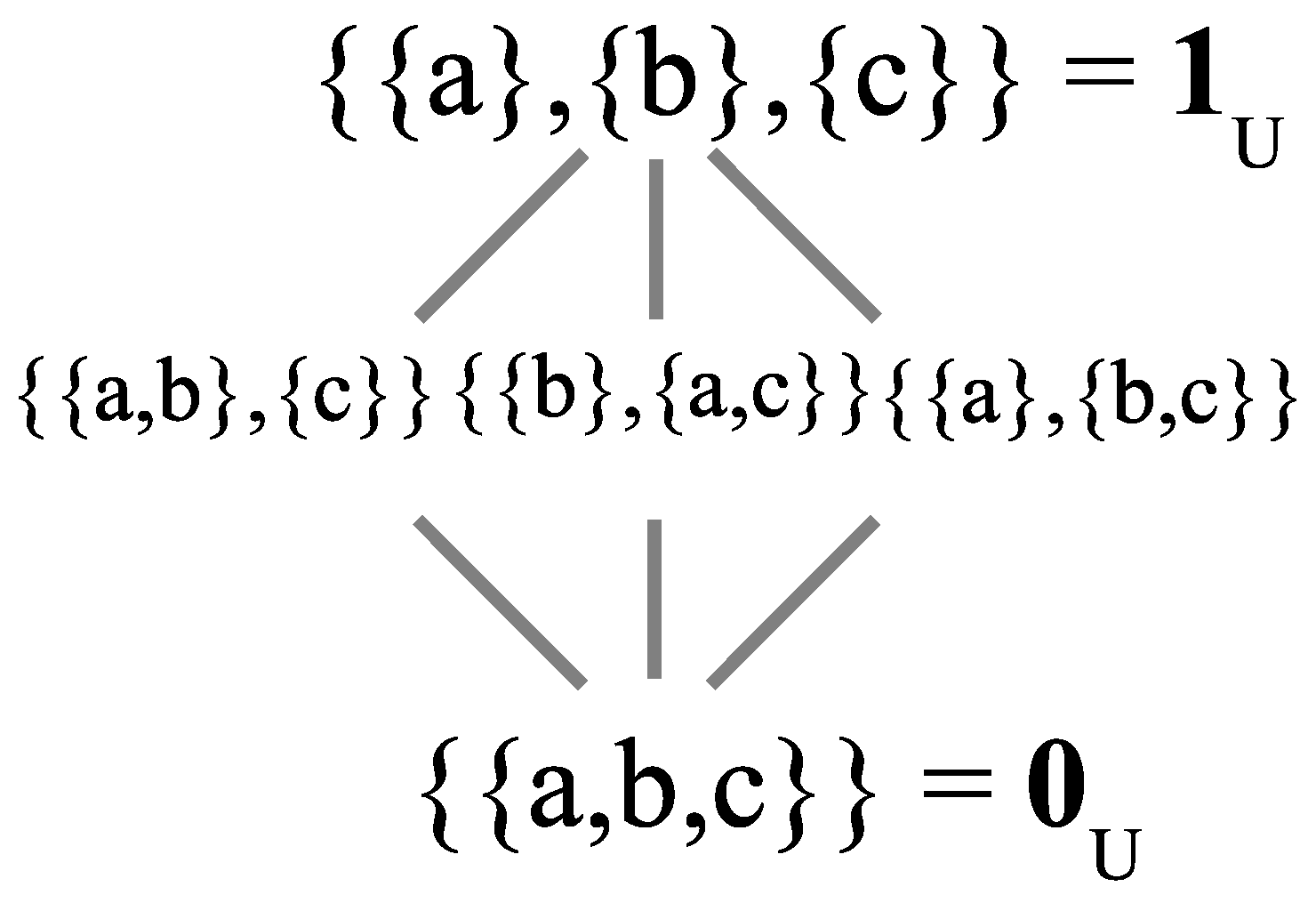
In this case, the more-mixed state is the density matrix for the discrete partition ${\mathbf{1}}_U$. This measurement operation is illustrated in Figure 3 where the change from $\rho \left(\pi \right)$ to $\widehat{\rho }\left(\pi \right)$ is indicated by the arrow from $\pi$ to ${\mathbf{1}}_U$. That movement from an indefinite state to a more definite state, like the arrow in Figure 3 is the skeletal representation of the infamous quantum jump in full QM.

Figure 3. Illustration of measurement (or state reduction) as a join operation.

It is easily shown in the general case, [1], that:

$$\widehat{\rho }\left(\pi \right)=\rho \left(\pi \vee g^{-1}\right),$$

namely, that in QM/Sets, the projective measurement operation is just the partition join, where one partition represents the state being measured, and the other partition represents the measurement that is observable or numerical attribute.

3.8. A New Information Measure: Logical Entropy

There is a natural notion of ‘classical’ and quantum entropy based on the notion of information as distinctions or distinguishings. As Charles Bennett, one of the founders of quantum information theory put it, “information really is a very useful abstraction. It is the notion of distinguishability abstracted away from what we are distinguishing, or from the carrier of information….” [14] (p. 155) Ordinary logic is based on the Boolean logic of subsets (usually presented in the special case of propositional logic). The notion of a subset is category-theoretically dual to the notion of a partition, and there is a dual logic of partitions [2]. The quantitative version of Boole’s logic of subsets started as finite ‘logical’ probability theory [15] with equiprobable outcomes, i.e., $\mathrm{Pr}\left(S\right)=\frac{\left|S\right|}{\left|U\right|}$, the normalized number of elements in a subset or event. In the duality between subsets and partitions, distinctions of a partition are dual to elements of a subset. Hence, the quantitative notion of a partition is the normalized number of distinctions, and that is the first definition of logical entropy [16,17] with equiprobable outcomes:

$$h\left(\pi \right)=\frac{\left|\mathrm{dit}\left(\pi \right)\right|}{\left|U\times U\right|}=\frac{\left|U\times U-{\Sigma }_j\left(B_j\times B_j\right)\right|}{\left|U\times U\right|}=1-{\sum }_j{\left(\frac{\left|B_j\right|}{\left|U\right|}\right)}^2=1-{\sum }_j\mathrm{Pr}{\left(B_j\right)}^2$$

where $\mathrm{Pr}\left(B_j\right)=\frac{\left|B_j\right|}{\left|U\right|}$ in this equiprobable case. In the general case of point probabilities, $\mathrm{Pr}\left(B_j\right)={\sum }_{u_i\in B_j}{p}_i$ and

$$h\left(\pi \right)=1-{\sum }_j\mathrm{Pr}{\left(B_j\right)}^2={\sum }_{j\ne j^{\prime }}\mathrm{Pr}\left(B_j\right)\mathrm{Pr}\left(B_{j^{\prime }}\right)$$

where the last equation holds since $1={\left({\sum }_{j=1}^m\mathrm{Pr}\left(B_j\right)\right)}^2={\sum }_j\mathrm{Pr}{\left(B_j\right)}^2+{\sum }_{j\ne j^{\prime }}\mathrm{Pr}\left(B_j\right)\mathrm{Pr}\left(B_{j^{\prime }}\right)$.

The logical entropy has a natural interpretation; just as $\mathrm{Pr}\left(S\right)={\sum }_{u_i\in S}{p}_i$ is the probability that one random draw from U will yield an element of S, so $h\left(\pi \right)$ is the probability that two random draws from U will yield a distinction of $\pi$. The information in a partition $\pi$ is reproduced in the density matrix $\rho \left(\pi \right)$, and the logical entropy can thus be calculated in terms of the density matrix:

$$h\left(\pi \right)=1-{\sum }_j\mathrm{Pr}{\left(B_j\right)}^2=1-\mathrm{tr}\left[\rho {\left(\pi \right)}^2\right]=h\left(\rho \left(\pi \right)\right)$$

i.e., as one minus the trace of the density matrix squared–which is the matrix version of $1-{\sum }_j\mathrm{Pr}{\left(B_j\right)}^2$.

For our purposes at hand, the important thing is that logical entropy measures the increase in information-as-distinctions that takes place in projective measurement. In general, the ditset of a join is just the union of the ditsets of two partitions, i.e., $\mathrm{dit}\left(\pi \vee \sigma \right)=\mathrm{dit}\left(\pi \right)\cup \mathrm{dit}\left(\sigma \right)$. Thus, projective measurement will, in general, increase the logical entropy of the state being measured. And since logical entropy is based on information-as-distinctions, and the density matrix represents distinctions as the zero entries, the increase in logical entropy can be calculated directly from the new zero entries in the post-measurement density matrix $\widehat{\rho }\left(\pi \right)$ compared to pre-measurement $\rho \left(\pi \right)$. The “measuring measurement theorem” in both the simplified pedagogical model of QM/Sets and in the full QM version is that the increase in logical entropy due to a projective measurement is the sum of the (absolute) squares of the non-zero entries (i.e., coherences) in the pre-measurement density matrix that are zeroed (i.e., decohered) in the post-measurement density matrix.

In the example, the two logical entropies are:

$$\begin{array}{c}h\left(\rho \left(\pi \right)\right)=1-\mathrm{tr}\left[\rho {\left(\pi \right)}^2\right]=1-\mathrm{tr}\left[{\left[\begin{array}{ccc}\frac{1}{2}& 0& \frac{1}{2\sqrt{3}}\\ 0& \frac{1}{3}& 0\\ \frac{1}{2\sqrt{3}}& 0& \frac{1}{6}\end{array}\right]}^2\right]=1-\mathrm{tr}\left[\left[\begin{array}{ccc}\frac{1}{3}& 0& \frac{\sqrt{3}}{9}\\ 0& \frac{1}{9}& 0\\ \frac{\sqrt{3}}{9}& 0& \frac{1}{9}\end{array}\right]\right]=\\ 1-\frac{5}{9}=\frac{4}{9}\mathrm{and}\\ h\left(\widehat{\rho }\left(\pi \right)\right)=1-\mathrm{tr}\left[\widehat{\rho }\left(\pi \right)\right]=1-\mathrm{tr}\left[{\left[\begin{array}{ccc}\frac{1}{2}& 0& 0\\ 0& \frac{1}{3}& 0\\ 0& 0& \frac{1}{6}\end{array}\right]}^2\right]=1-\mathrm{tr}\left[\left[\begin{array}{ccc}\frac{1}{4}& 0& 0\\ 0& \frac{1}{9}& 0\\ 0& 0& \frac{1}{36}\end{array}\right]\right]=1-\frac{14}{36}=\frac{11}{18}.\end{array}$$

In the transition from $\rho \left(\pi \right)$ to $\widehat{\rho }\left(\pi \right)$, only two entries of $\frac{1}{2\sqrt{3}}$ were zeroed. The sum of their squares is $\frac{2}{12}=\frac{1}{6}$, and the increase in logical entropy is $h\left(\widehat{\rho }\left(\pi \right)\right)-h\left(\rho \left(\pi \right)\right)=\frac{11}{18}-\frac{8}{18}=\frac{3}{18}=\frac{1}{6}$. These results in QM/Sets enriched with density matrices are the simplified version of the corresponding results in full QM [16] (p. 83).

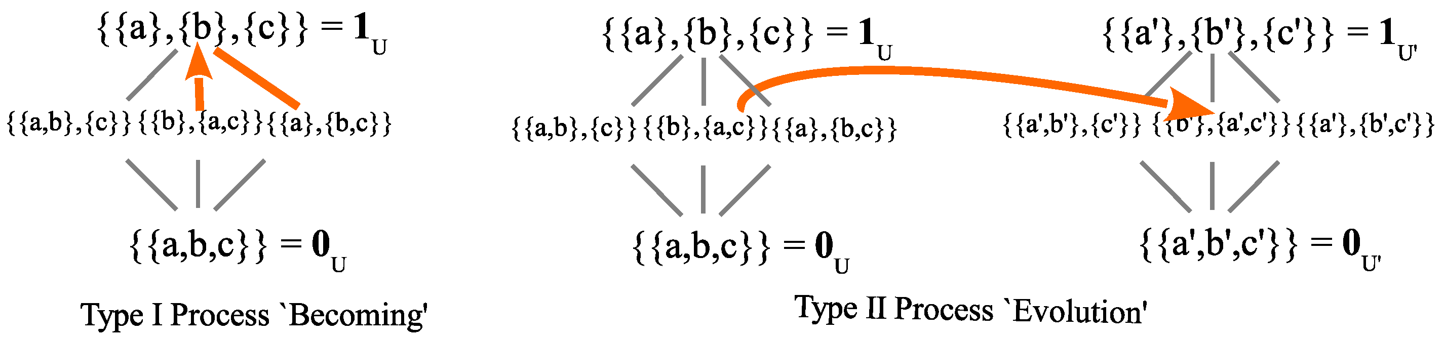
3.9. Quantum Processes

John von Neumann famously divided quantum processes into two types [18]. Type I was the process of measurement (state reduction), which we have seen involves the making of distinctions to transform an indefinite state into a more definite state. This is the quantum notion of “becoming”. The Type II processes were the solutions to the time-dependent Schrödinger equation. But how might the Type II processes be characterized using the notion of information-as-distinctions? Since the Type I processes make distinctions, the simplest description of Type II processes would be ones that do not make distinctions. The extent to which two normalized states $\left|\psi \right.⟩$ and $\left|\varphi \right.⟩$ in QM are distinguished is given by their inner product $⟨\varphi |\psi ⟩$; if $⟨\varphi |\psi ⟩=0$, they are maximally distinct (i.e., orthogonal), and if $⟨\varphi |\psi ⟩=1$, they are not distinguished. Hence the natural description of Type II processes is one that does not change the distinctness of quantum states, i.e., that preserve the inner product, which are the unitary transformations. The connection to the solutions of Schrödinger’s equation is given by Stone’s Theorem [19].

One of the controversial aspects of the Type I measurement process is its indeterminancy. The Lüder mixture operation turns a pure (or mixed) state being measured into a mixed (or more mixed) state, and then one of the states in the mixture occurs, according to its probability. The transformation from the pre-measurement state to the post-measurement state is not unitary; it is a “state reduction”. It is known in misleading and archaic language as “collapse of the wave packet”. In the previous example in QM/Sets, measurement turned the mixed state $\pi =\left\{\left\{b\right\},\left\{a,c\right\}\right\}$ into the more mixed state ${\mathbf{1}}_U=\left\{\left\{a\right\},\left\{b\right\},\left\{c\right\}\right\}$. There is no indeterminacy in $\left\{b\right\}⇝\left\{b\right\}$; the indeterminacy is in $\left\{a,c\right\}⇝\left\{a\right\}$ or $\left\{a,c\right\}⇝\left\{c\right\}$.

This indeterminacy comes out clearly at the set level in the notion of a “choice function” [20] (p. 60). In axiomatic set theory, the axiom of choice states that for any set of non-empty sets, there is a choice function for it. Given a set of non-empty sets, a choice function takes each non-empty set to one of its elements. In QM, there is no indeterminacy in the measurement of an eigenstate in the measurement basis; the result is that eigenstate with probability one. Similarly, there is no indeterminacy in a choice function applied to a singleton, e.g., $\left\{b\right\}⇝\left\{b\right\}$. The indeterminacy arises in set theory only when the choice is made out of a multiple-element set, e.g., $\left\{a,c\right\}⇝\left\{c\right\}$. Similarly, the indeterminacy arises in QM only when the measurement is made of a state that is a superposition (in the measurement basis). Perhaps this is a case where the set version of a QM operation helps to remove some of the ‘mystery’, e.g., in what is called the “collapse postulate”.

What is the QM/Sets version of a unitary transformation since there are no inner products in vector spaces over finite fields like ${\mathbb{Z}}_2$? A unitary transformation can be defined as a linear transformation that takes an orthonormal basis to an orthonormal basis. Hence, the corresponding transformation for ${\mathbb{Z}}_2^n$ would be a linear transformation that takes a basis set to a basis set–which is simply a non-singular linear transformation. For instance, using the U-basis and the $U^{\prime }$-basis of Table 1, the transformation defined by $\left\{a\right\}⇝\left\{a^{\prime }\right\}=\left\{a,b\right\}$, $\left\{b\right\}⇝\left\{b^{\prime }\right\}=\left\{a,b,c\right\}$, and $\left\{c\right\}⇝\left\{c^{\prime }\right\}=\left\{b,c\right\}$ is a non-singular linear transformation that takes the U-basis to the $U^{\prime }$-basis. It might be noted that such non-singular transformations do preserve the value of the brackets when we take into account their basis-dependency. For instance, if the sets $S,T\subseteq U$ of U-basis elements transform into the corresponding sets $S^{\prime },T^{\prime }\subseteq U^{\prime }$ in the $U^{\prime }$-basis, then $⟨{S|}_{U}T⟩=⟨S^{\prime }{|}_{U^{\prime }}{T}^{\prime }⟩$. Such non-singular linear transformations on ${\mathbb{Z}}_2^n$ are the QM/Sets version of the Type II quantum processes.

The Type I processes of becoming were represented in a skeletal form on the left-hand side, and the Type II processes of evolution can be applied to pure or mixed states on the right-hand side in Figure 4. The arrow on the right-hand side pictures the transformation of the mixed state $\left\{\left\{b\right\},\left\{a,c\right\}\right\}$ into the mixed state $\left\{\left\{b^{\prime }\right\},\left\{a^{\prime },c^{\prime }\right\}\right\}=\left\{\left\{a,b,c\right\},\left\{a,c\right\}\right\}$.

Figure 4. Anschaulich (intuitive) model of Type I and Type II processes using partition lattices.

The very important thing to notice about the Type II transformations is that they can operate on pure states or mixed states involving superpositions like $\left\{a,c\right\}$; they do not just operate on fully distinguished states like ${\mathbf{1}}_U⇝{\mathbf{1}}_{U^{\prime }}$ like in classical physics. We see in Figure 4 why there are two fundamental processes in QM: Type I (making an indefinite state more definite) and Type II (transforming a state to another state at the same level of indefiniteness).

Some quantum philosophers have questioned how there can be two fundamental processes in QM when there is only one in classical physics since “it seems unbelievable that there is a fundamental distinction between “measurement” and “non-measurement” processes. Somehow, the true fundamental theory should treat all processes in a consistent, uniform fashion” [21] (p. 245). Our analysis gives an explanation why there is only one fundamental process (transforming definite states into definite states) in classical mechanics—in terms of the two processes in QM. When is the Type I process no longer possible? There can be no transformation of indefinite to more definite if the state is already fully definite, i.e., in a classical mixed state represented by ${\mathbf{1}}_U$. Then only the Type II process of transforming definite states into definite states is possible, as in classical mechanics.

As we will also see in the QM/Sets treatment of the double-slit experiment, that aspect is the key to understanding how a particle in the superposition state $\left|\mathrm{Slit}1\right.⟩+\left|\mathrm{Slit}2\right.⟩$ can evolve without first becoming the more-definite states of $\left|\mathrm{Slit}1\right.⟩$ or $\left|\mathrm{Slit}2\right.⟩$, i.e., can evolve without going through Slit 1 or going through Slit 2. And it is that evolution of the superposition that involves the characteristic interference effects.

3.10. The Double-Slit Experiment in QM/Sets

We focus on the double-slit experiment since, according to Feynman, “it contains the only mystery” and it illustrates “the basic peculiarities of quantum mechanics” [22] (Section 1-1).

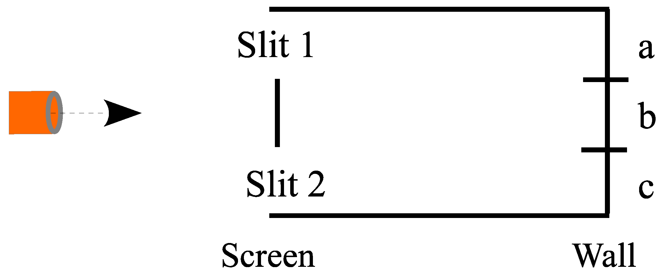
To model the essential aspects (and only those aspects), we consider the setup in Figure 5 where the three states in $U=\left\{a,b,c\right\}$ stand for vertical positions. A particle is sent from $\left\{b\right\}$ towards a screen with two slits in it at positions $\left\{a\right\}$ and $\left\{c\right\}$. The dynamics are the aforementioned transformations of the U-basis into the $U^{\prime }$-basis each time period. One time period takes the particle to the screen, and the next time period takes the particle to the wall.

Figure 5. Setup for the two-slit experiment model in QM/Sets.

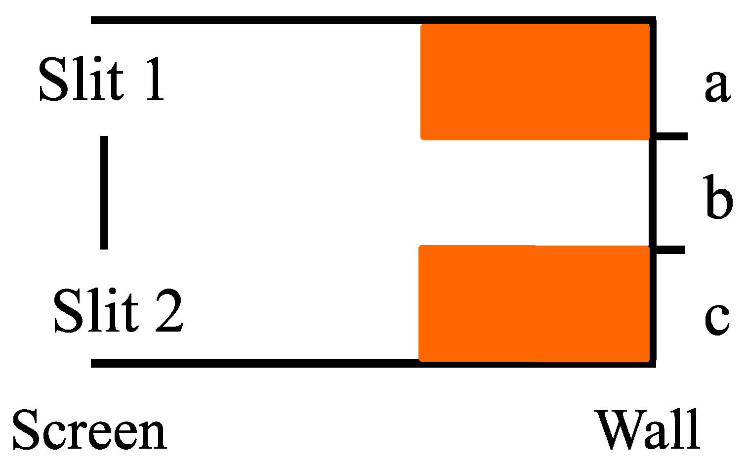
In the first time period, the particle evolves $\left\{b\right\}⇝\left\{b^{\prime }\right\}=\left\{a,b,c\right\}$. One-third of the time the particle hits the barrier between the slits; we are concerned with the alternative case where the particle’s state is reduced to the superposition state $\left|\mathrm{Slit}1\right.⟩+\left|\mathrm{Slit}2\right.⟩$, which in the model is $\left\{a,c\right\}$. Then there are two cases to consider: Case 1 of detection at the slits, and Case 2 of no detection at the slits–both starting with $\left\{a,c\right\}$ at the screen.

Case 1. With detection at the slits, the superposition state $\left\{a,c\right\}$ is reduced to $\left\{a\right\}$ (i.e., going through Slit 1) with probability $\frac{1}{2}$ or to $\left\{c\right\}$ (i.e., going through Slit 2) with probability $\frac{1}{2}$ so we have:

$$\mathrm{Pr}\left(\left\{a\right\}\mathrm{at}\mathrm{screen}|\left\{a,c\right\}\right)=\frac{1}{2}=\mathrm{Pr}\left(\left\{c\right\}|\left\{a,c\right\}\right)=\frac{\left|\left\{a\right\}\cap \left\{a,c\right\}\right|}{\left|\left\{a,c\right\}\right|}.$$

Then in the next time period, we have either $\left\{a\right\}$ evolving to $\left\{a^{\prime }\right\}=\left\{a,b\right\}$ and hitting the detection wall at $\left\{a\right\}$ or $\left\{b\right\}$ each with probability $\frac{1}{2}$, or similarly, $\left\{c\right\}$ evolving to $\left\{b,c\right\}$ and hitting the wall at $\left\{b\right\}$ or $\left\{c\right\}$ each with probability $\frac{1}{2}$. Then the computation of the probabilities to reach the three positions at the wall are as follows:

$$\begin{array}{c}\mathrm{Pr}\left(\left\{a\right\}\mathrm{at}\mathrm{wall}|\left\{a,b\right\}\mathrm{at}\mathrm{wall}\right)\mathrm{Pr}\left(\left\{a\right\}\mathrm{at}\mathrm{screen}|\left\{a,c\right\}\right)\hfill \\ +\mathrm{Pr}\left(\left\{a\right\}\mathrm{at}\mathrm{wall}|\left\{b,c\right\}\mathrm{at}\mathrm{wall}\right)\mathrm{Pr}\left(\left\{c\right\}\mathrm{at}\mathrm{screen}|\left\{a,c\right\}\right)\hfill \\ =\frac{\left|\left\{a\right\}\cap \left\{a,b\right\}\right|}{\left|\left\{a,b\right\}\right|}\frac{\left|\left\{a\right\}\cap \left\{a,c\right\}\right|}{\left|\left\{a,c\right\}\right|}+\frac{\left|\left\{a\right\}\cap \left\{b,c\right\}\right|}{\left|\left\{b.c\right\}\right|}\frac{\left|\left\{c\right\}\cap \left\{a,c\right\}\right|}{\left|\left\{a,c\right\}\right|}=\frac{1}{2}\times \frac{1}{2}+0\times \frac{1}{2}=\frac{1}{4};\hfill \\ \mathrm{Pr}\left(\left\{b\right\}\mathrm{at}\mathrm{wall}|\left\{a.b\right\}\mathrm{at}\mathrm{wall}\right)\mathrm{Pr}\left(\left\{a\right\}\mathrm{at}\mathrm{screen}|\left\{a,c\right\}\right)\hfill \\ +\mathrm{Pr}\left(\left\{b\right\}\mathrm{at}\mathrm{wall}|\left\{b,c\right\}\mathrm{at}\mathrm{wall}\right)\mathrm{Pr}\left(\left\{c\right\}\mathrm{at}\mathrm{screen}|\left\{a,c\right\}\right)\hfill \\ =\frac{\left|\left\{b\right\}\cap \left\{a,b\right\}\right|}{\left|\left\{a,b\right\}\right|}\frac{\left|\left\{a\right\}\cap \left\{a,c\right\}\right|}{\left|\left\{a,c\right\}\right|}+\frac{\left|\left\{b\right\}\cap \left\{b,c\right\}\right|}{\left|\left\{b.c\right\}\right|}\frac{\left|\left\{c\right\}\cap \left\{a,c\right\}\right|}{\left|\left\{a,c\right\}\right|}=\frac{1}{2}\times \frac{1}{2}+\frac{1}{2}\times \frac{1}{2}=\frac{1}{2};\hfill \\ \mathrm{Pr}\left(\left\{c\right\}\mathrm{at}\mathrm{wall}|\left\{b,c\right\}\mathrm{at}\mathrm{wall}\right)\mathrm{Pr}\left(\left\{c\right\}\mathrm{at}\mathrm{screen}|\left\{a,c\right\}\right)\hfill \\ +\mathrm{Pr}\left(\left\{c\right\}\mathrm{at}\mathrm{wall}|\left\{a,b\right\}\mathrm{at}\mathrm{wall}\right)\mathrm{Pr}\left(\left\{a\right\}\mathrm{at}\mathrm{screen}|\left\{a,c\right\}\right)\hfill \\ =\frac{\left|\left\{c\right\}\cap \left\{b,c\right\}\right|}{\left|\left\{b,c\right\}\right|}\frac{\left|\left\{c\right\}\cap \left\{a,c\right\}\right|}{\left|\left\{a,c\right\}\right|}+\frac{\left|\left\{c\right\}\cap \left\{a,b\right\}\right|}{\left|\left\{a,b\right\}\right|}\frac{\left|\left\{a\right\}\cap \left\{a,c\right\}\right|}{\left|\left\{a,c\right\}\right|}=\frac{1}{2}\times \frac{1}{2}+0\times \frac{1}{2}=\frac{1}{4}.\hfill \end{array}$$

The resulting probability distribution is pictured in Figure 6.

Figure 6. Case 1 of probability distribution of hits at wall from detection at the slits.

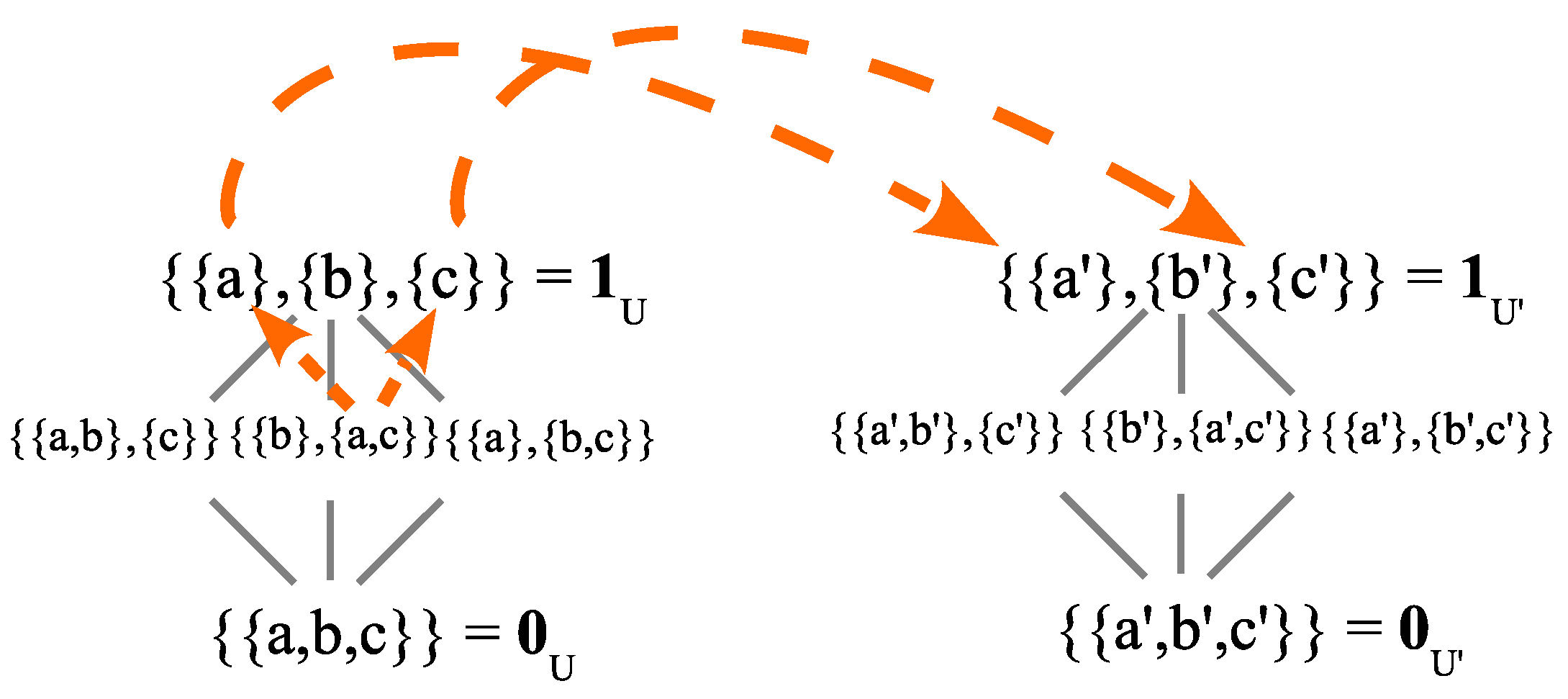
In Case 1, the detection at the slits forces the state reduction of $\left\{a,c\right\}$ to either $\left\{a\right\}$ (i.e., going through slit 1) or $\left\{c\right\}$ (i.e., going through slit 2), and then one or the other evolves respectively to $\left\{a^{\prime }\right\}=\left\{a,b\right\}$ or $\left\{c^{\prime }\right\}=\left\{b,c\right\}$. These state reductions and evolutions are (dashed arrows) illustrated in Figure 7.

Figure 7. State reductions and evolutions in Case 1.

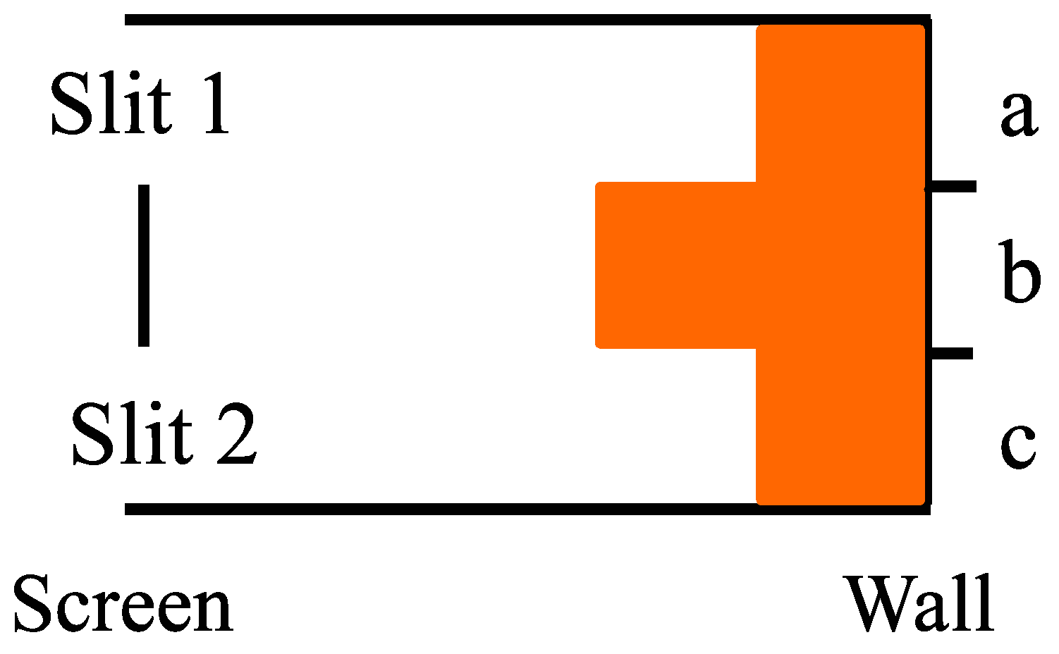
Case 2. With no detection at the slits, the superposition state $\left\{a,c\right\}$ evolves as an indefinite or superposition state since there was no state reduction at the slits. Hence, the evolution is:

$$\left\{a,c\right\}⇝\left\{a^{\prime },c^{\prime }\right\}=\left\{a^{\prime }\right\}+\left\{c^{\prime }\right\}=\left\{a,b\right\}+\left\{b,c\right\}=\left\{a,c\right\}.$$

Then the probability distribution for the hits at the wall are as follows:

$$\begin{array}{c}\mathrm{Pr}\left(\left\{a\right\}\mathrm{at}\mathrm{wall}|\left\{a,c\right\}\mathrm{at}\mathrm{wall}\right)\mathrm{Pr}\left(\left\{a,c\right\}\mathrm{at}\mathrm{wall}|\left\{a,c\right\}\right)=\frac{\left|\left\{a\right\}\cap \left\{a,c\right\}\right|}{\left|\left\{a,c\right\}\right|}\frac{\left|\left\{a,c\right\}\cap \left\{a,c\right\}\right|}{\left|\left\{a,c\right\}\right|}=\frac{1}{2}\times 1=\frac{1}{2};\hfill \\ \mathrm{Pr}\left(\left\{b\right\}\mathrm{at}\mathrm{wall}|\left\{a,c\right\}\mathrm{at}\mathrm{wall}\right)\mathrm{Pr}\left(\left\{a,c\right\}\mathrm{at}\mathrm{wall}|\left\{a,c\right\}\right)=\frac{\left|\left\{b\right\}\cap \left\{a,c\right\}\right|}{\left|\left\{a,c\right\}\right|}\frac{\left|\left\{a,c\right\}\cap \left\{a,c\right\}\right|}{\left|\left\{a,c\right\}\right|}=0\times 1=0;\hfill \\ \mathrm{Pr}\left(\left\{c\right\}\mathrm{at}\mathrm{wall}|\left\{a,c\right\}\mathrm{at}\mathrm{wall}\right)\mathrm{Pr}\left(\left\{a,c\right\}\mathrm{at}\mathrm{wall}|\left\{a,c\right\}\right)=\frac{\left|\left\{c\right\}\cap \left\{a,c\right\}\right|}{\left|\left\{a,c\right\}\right|}\frac{\left|\left\{a,c\right\}\cap \left\{a,c\right\}\right|}{\left|\left\{a,c\right\}\right|}=\frac{1}{2}\times 1=\frac{1}{2}.\hfill \end{array}$$

The resulting probability distribution is pictured in Figure 8.

Figure 8. Case 2 of probability distribution of hits at wall with no detection at the slits.

Figure 8 shows the stripes characteristic of the interference pattern, i.e., $\left\{a,b\right\}+\left\{b,c\right\}=\left\{a,c\right\}$, resulting from no detection at the slits.

The hardest point to understand is that our classical intuitions ‘insist’ that the particle has to go through Slit 1 or Slit 2 (which would yield the Figure 6 distribution of hits), but the distribution is as in Figure 8 showing the stripes resulting from interference. The problem with our classical intuitions is that they operate at the classical level of all states being distinguished from each other (i.e., no superpositions), so one or the other of the distinguished states “going through Slit 1” and “going through Slit 2” has to occur. In the quantum notion of becoming, states are constructed from below, as it were, by making distinctions to go from indefinite to more definite states. 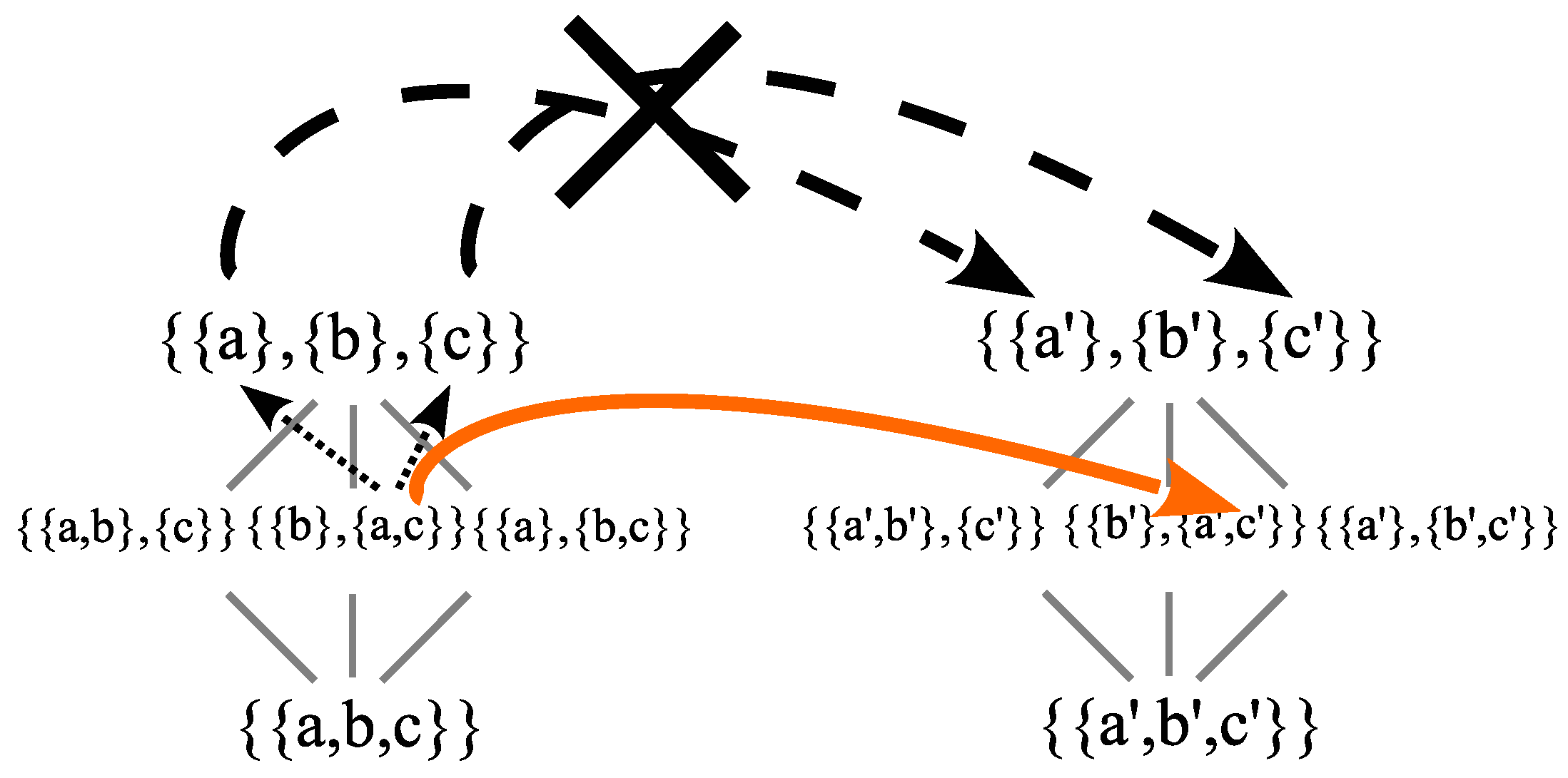But the indefinite state $\left\{a,c\right\}$ was not distinguished in Case 2. The classical level evolution of the distinguished states that do not occur in Case 2 is marked with an X in Figure 9. As Richard Feynman put it: “We must conclude that when both holes are open, it is not true that the particle goes through one hole or the other” [23] (p. 536).

Figure 9. The evolution of distinguished states $\left\{a\right\}$ or $\left\{c\right\}$ does not occur in Case 2.

But with no distinction at the slits in Case 2, it is the non-classical superposition state $\left|\mathrm{Slit}1\right.⟩+\left|\mathrm{Slit}2\right.⟩$, or $\left\{a,c\right\}$ in the model that evolves, which incurs the cancellation in the linear non-singular transformation resulting in the interference stripes of Figure 8:

$$\left\{a,c\right\}=\left\{a\right\}+\left\{c\right\}⇝\left\{a^{\prime }\right\}+\left\{c^{\prime }\right\}=\left\{a,b\right\}+\left\{b,c\right\}=\left\{a,c\right\}.$$

That is how the particle can ultimately hit the wall without going through one of the slits, i.e., without the state reductions $\left\{a,c\right\}⇝\left\{a\right\}$ (going through slit 1) or $\left\{a,c\right\}⇝\left\{c\right\}$ (going through slit 2). Distinguishing between the alternatives in an interaction involving a superposition will wipe out any interference effects, i.e., will give Case 1 instead of Case 2.

Any determination of the alternative taken by a process capable of following more than one alternative destroys the interference between alternatives.

([24], p. 9)

The lattice of partitions gives a skeletal representation of the rising levels of definiteness going from the bottom to the top. The top represents the fully definite or distinguished states. In Case 2, the evolution takes place at a lower level, a level of indefiniteness where those states $\left\{a,c\right\}$ are not distinguished. In classical physics, all states are distinguished, so classical evolution always takes definite states to definite states (as in the evolution marked by X in Figure 9). Here we see, in terms of the simplified model, the answer to the key question: “How does the particle get to the detection wall without passing through slit 1 or slit 2?”.

3.11. The Feynman Rules

3.11.1. The Fundamental Role of Distinguishability

The formulation of QM that shows the fundamental role of distinctions or distinguishings was developed by Richard Feynman [24] who encapsulated the rules for working with amplitudes in the “Feynman rules” ([6,25] (pp. 314–315)) such as the one involved in analyzing the double-slit experiment.

The probability of an event (in an ideal experiment where there are no uncertain external disturbances) is the absolute square of a complex quantity called the probability amplitude. When the event can occur in several alternative ways, the probability amplitude is the sum of the probability amplitude for each alternative considered separately…. If an experiment capable of determining which alternative is actually taken is performed, the interference is lost and the probability becomes the sum of the probability for each alternative.

([23], p. 538)

John Stachel gives the application to the double-slit experiment.

Feynman’s approach is based on the contrast between processes that are distinguishable within a given physical context and those that are indistinguishable within that context. A process is distinguishable if some record of whether or not it has been realized results from the process in question; if no record results, the process is indistinguishable from alternative processes leading to the same end result. In my terminology, a registration of the realization of a process must exist for it to be a distinguishable alternative. In the two-slit experiment, for example, passage through one slit or the other is only a distinguishable alternative if a counter is placed behind one of the slits; without such a counter, these are indistinguishable alternatives. Classical probability rules apply to distinguishable processes. Nonclassical probability amplitude rules apply to indistinguishable processes.

([25], p. 314)

In QM/Sets, the ‘amplitudes’ are given by the vectors in the vector space over ${\mathbb{Z}}_2$ where the cancellations occur, e.g., $\left\{a,b\right\}+\left\{b,c\right\}=\left\{a,c\right\}$, in the non-distinguished Case 2, and then the probabilities are computed from the resulting amplitudes by the Born rule. In the distinguished Case 1, the probabilities from the distinct alternatives are added, e.g., the probabilities of the two distinct ways of $\left\{a,c\right\}$ at the screen eventually resulting in $\left\{b\right\}$ at the wall are added:

$$\begin{array}{c}\mathrm{Pr}\left(\left\{b\right\}\mathrm{at}\mathrm{wall}|\left\{a.b\right\}\mathrm{at}\mathrm{wall}\right)\mathrm{Pr}\left(\left\{a\right\}\mathrm{at}\mathrm{screen}|\left\{a,c\right\}\right)+\\ \mathrm{Pr}\left(\left\{b\right\}\mathrm{at}\mathrm{wall}|\left\{b,c\right\}\mathrm{at}\mathrm{wall}\right)\mathrm{Pr}\left(\left\{c\right\}\mathrm{at}\mathrm{screen}|\left\{a,c\right\}\right)=\frac{1}{2}\frac{1}{2}+\frac{1}{2}\frac{1}{2}=\frac{1}{2}.\end{array}$$

By following the Feynman rules, probabilities can be computed without “being confused by things such as the ‘reduction of a wave packet’ and similar magic” [26] (p. 76). Using the rules to calculate probabilities, of course, does not eliminate state reductions since “a registration of the realization of a process must exist for it to be a distinguishable alternative” [25] (p. 314). The point is what causes the state reduction, namely the distinguishability of the previously superposed alternatives undergoing an interaction.

3.11.2. Weyl’s Use of the Yoga

In his popular writing about QM, Arthur Eddington used the notion of a sieve.

In Einstein’s theory of relativity, the observer is a man who sets out in quest of truth, armed with a measuring rod. In quantum theory, he sets out armed with a sieve.

([27], p. 267)

Hermann Weyl quotes Eddington about the idea of a sieve, which Weyl calls a “grating” [8] (p. 255). Weyl then, in effect, uses the Yoga of linearization to develop the idea of a grating both as a set partition (or equivalence relation) and as a vector space direct-sum decomposition (DSD) [8] (pp. 255–257). He starts with a numerical attribute, e.g., $g:U\to \mathbb{R}$, which defines a partition on a set or “aggregate [which] is used in the sense of ‘set of elements with equivalence relation’” [8] (p. 239). Then he goes to the quantum case where the “aggregate of n states has to be replaced by an n-dimensional Euclidean vector space” [8] (p. 256. “Euclidean” is older terminology for an inner product space). He describes the vector space notion of a grating as the “splitting of the total vector space into mutually orthogonal subspaces” so that “each vector $\overrightarrow{x}$ splits into r component vectors lying in the several subspaces” [8] (p. 256), i.e., a direct-sum decomposition of the space. 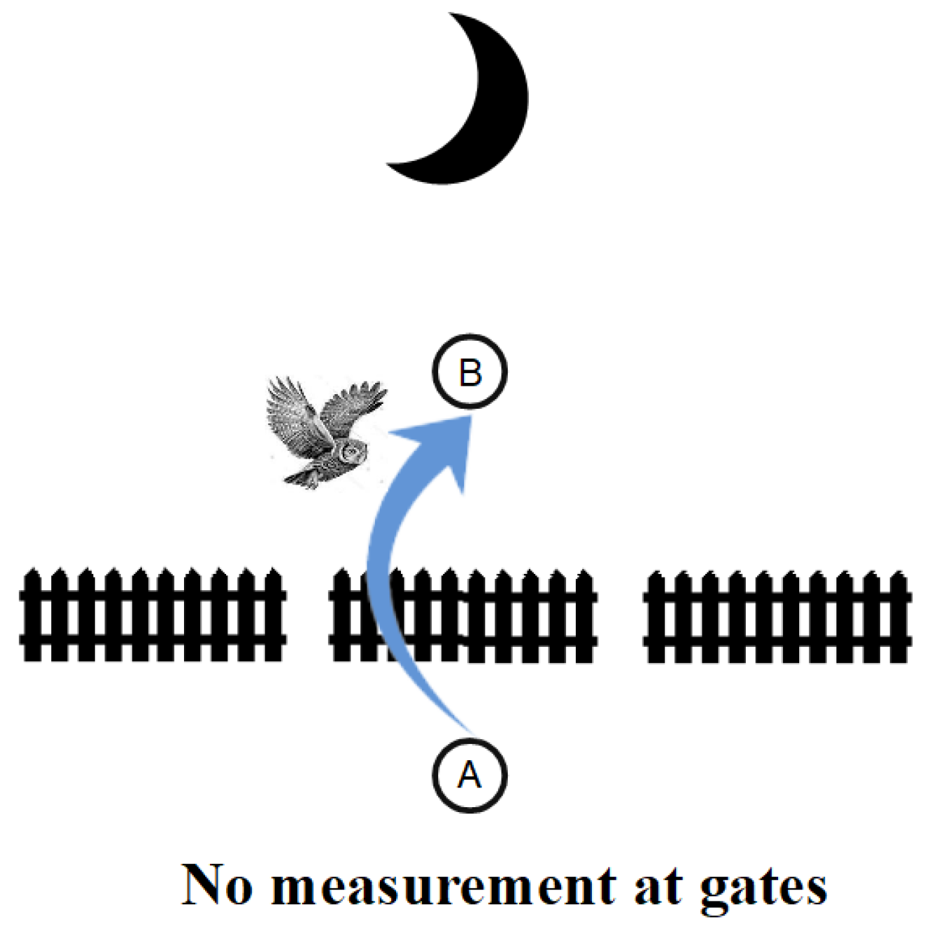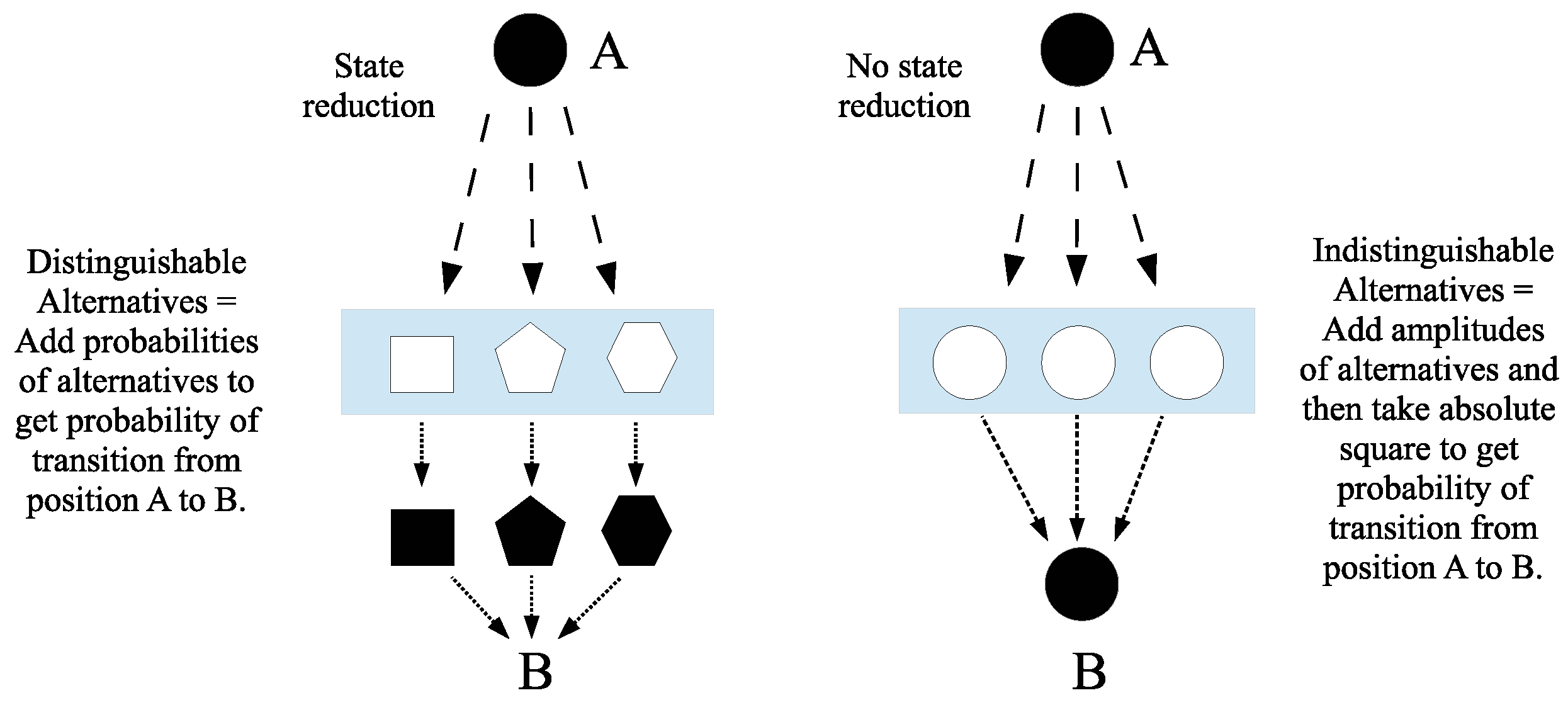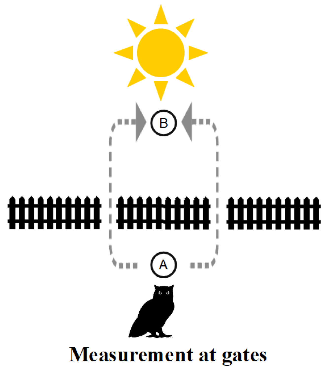Finally, Weyl notes that “Measurement means application of a sieve or grating” [8] (p. 259). In Figure 10, this idea of measurement as a superposition state passing through a grating or sieve is illustrated (on the left side) along with a similar image (on the right side) where no distinctions or distinguishings take place, so there is no measurement.

Figure 10. Visual illustration of Feynman’s rule with measurement seen as applying a grating.

The doughball-shaped figure at position A visually illustrates the superposition of the definite shapes in the left-side grating. As the doughball falls through one of the holes, it “collapses” or reduces from its indefinite or superposition state to one of the definite eigenstates. To get the total probability of going from A to B, one has to add the three probabilities of each distinguishable path from A to B. On the right side of Figure 10, no distinctions are made at a ‘null-grating’ so the amplitudes to go from A to B are added, and the (absolute) square gives the probability.

4. Discussion

4.1. Metaphors for the Quantum World

There are a number of (always imperfect) metaphors that might help to better visualize the quantum world as opposed to the classical world of fully definite or distinguished states.

• Flipping through a police mugbook, going from one definite face to another, is like change in classical physics going from one definite state to another. There is no ‘becoming’ (from indefinite to more definite) in the classical world; all states are fully definite.
• A police sketchpad illustrates Type I quantum-becoming, starting from an indefinite picture of a face and using witness information to make a more distinct and realistic face.
• Similarly, the painter starts with a white (= superposition of all colors) canvas and then becomes a painting as white spaces are ‘collapsed’ into definite colors.
• Perhaps another metaphor for the Type I process of becoming is the modern process of 3D printing. The object is constructed or printed from below and becomes more definite as more layers are printed.

Werner Heisenberg, in his more popular writings, was fond of formulating his philosophical thinking in terms of ancient Greek philosophy, e.g., the Aristotelian notions, such as substance and form.

Just as the Greeks had hoped, so we have now found there is only one fundamental substance of which all reality consists. If we have to give this substance a name, we can only call it ‘energy.’ But this fundamental ‘energy’ is capable of existence in different forms.

([28], p. 116)

He saw this energy substance as “a kind of indefinite corporeal substratum, embodying the possibility of passing over into actuality by means of the form” ([3], p. 148). This is a fine description of the Type I process of quantum becoming, where more definiteness is created through in-forming the substance with more information-as-distinctions, illustrated on the right side of Figure 11, by moving up the lattice of partitions from the pure unformed substance of the indiscrete partition at the bottom eventually to the fully in-formed discrete partition at the top. Given the duality of elements and distinctions, the quantum notion of becoming could be juxtaposed to the dual notion of becoming, illustrated on the left side of Figure 11, of moving from the bottom to the top of the Boolean lattice of subsets by the ex-nihilo creation of fully-formed elements of substance.

Figure 11. The two dual notions of becoming.

In the partition notion of becoming (Type I process), a quantum state $\pi$ is informed by the information-as-distinctions of an observable $g^{-1}$ to create the more-definite state of $\pi \vee g^{-1}$ with the new distinctions of $\mathrm{dit}\left(g^{-1}\right)-\mathrm{dit}\left(\pi \right)$. In cosmology, starting with the perfect symmetry [29] of the pre-Big Bang state, distinctions are created by symmetry-breaking. When a partition is formed by a group of symmetries, e.g., the orbit partition of a set representation of a group, then making a distinction (i.e., distinguishing between states previously equated as being symmetrical) takes the form of symmetry-breaking and moving to a smaller symmetry group with a more refined orbit partition.

Yet another metaphor is provided by Edwin Abbott’s Flatland fantasy [30], where creatures living in a two-dimensional world (like the classical world) find changes brought about using the third dimension (like the quantum world) to be unintuitive, if not incomprehensible. Kastner [31] uses the flatlander metaphor to make similar points. In the two-dimensional world, consider Hegel’s Owl of Minerva, who only flies at night [32] (p. 13), at point A facing a fence with two gates or slits in it. During the daytime, one can see (like detection at the slits in the double-slit experiment) which gate the owl has to walk through to get to point B on the other side, as illustrated in Figure 12.

Figure 12. With measurement at the gates, the Owl of Minerva has to go through one gate or the other.

But at night, it is like having no detection or observation at the slits in the double-slit experiment, then the Owl of Minerva takes to flight, i.e., has access to another realm of travel (like evolution in the indefinite quantum world) to get from A to B—as illustrated in Figure 13.

Figure 13. The Owl of Minerva takes advantage of the extra dimension to get from A to B.

Our classical-world intuitions correspond to the flatlander’s intuitions that the owl has to go through one gate or the other to get from A to B.

4.2. Whither Waves?

Other applications of QM/Sets include Bell’s Theorem. A treatment of Bell’s Theorem [33] intended for a popular audience can be reworked into QM/Sets. Still more applications include the treatment of indistinguishable particles and group representation theory [1]. But even this introduction to QM/Sets raises some interesting questions that go far beyond its pedagogical use.

For many years, quantum mechanics was called “wave mechanics”—although this usage is now largely in a welcome decline. The mathematics of QM is quite distinctive when compared to classical mechanics. But one must differentiate between the aspects of QM math that are essential and those that are more ‘incidental.’ One distinctive feature is that QM mathematics is formulated in Hilbert spaces over complex numbers. One might say the reason for this is that the complex numbers are algebraically complete so that all observable operators will have a full set of eigenvectors. ‘Coincidentally’, as it were, the complex numbers are the natural mathematics to describe waves, i.e., each complex number in its polar representation has an amplitude and a phase. Hence, QM mathematics abounds in wave-like machinery such as the Schrödinger wave equation and its wave-function solutions. Yet, quantum theorists have largely given up on seeing the wave function as a physical or ontic wave; it is only a “probability wave”, a computational device that allows the computation of probabilities by the Born rule. In terms of the attempts to understand the mysteries of QM, the ‘false leads’ of so-called “wave mechanics” may nuance Einstein’s famous saying that the “The Lord is subtle, but not malicious”. If not malicious, He at least seems to be a trickster.

As Feynman noted: “it must be emphasized that the wave function that satisfies the equation is not like a real wave in space; one cannot picture any kind of reality to this wave as one does for a sound wave” [22] (Section 3.7). In this respect, the classroom ripple-tank model of the two-slit experiment is seriously misleading. Those water waves are matter waves; the ‘waves’ of the wave functions are not. Moreover, in the absence of detection at the slits, the particle does not “go through both slits” (like ‘the wave’ is pictured as doing); instead, the superposition evolves at a non-classical level of indefiniteness. In that case, the particle does not rise to the definiteness of going through one slit or the other, not to mention both. The treatment of the double-slit experiment in QM/Sets explains the results without using the misleading mathematical machinery of waves, machinery that is necessarily there when working in a vector space over $\mathbb{C}$ instead of ${\mathbb{Z}}_2$. Instead of the so-called “wave-particle duality”, a quantum particle is in an indefinite superposition state or is in a definite- or eigen-state.

I want to emphasize that light comes in this form–particles. It is very important to know that light behaves like particles, especially for those of you who have gone to school, where you were probably told something about light behaving like waves. I am telling you the way it behaves–like particles.

([26], p. 15)

The constructive or destructive interference is not just a so-called “wave phenomena”; it occurs in the addition of vectors over any field whatsoever, from $\mathbb{C}$ to ${\mathbb{Z}}_2$. We have seen how so much of the essential structure and relationships (e.g., double-slit experiment) can be expressed in the simplified model of QM/Sets (i.e., QM over ${\mathbb{Z}}_2$, not $\mathbb{C}$) without any $\mathbb{C}$-based wave-math whatsoever. This is another difficult point to understand. The $\mathbb{C}$-based wave-math is not wrong but does not describe ontic waves, and that is why the “wave mechanics” interpretation has been misleading for a century. By seeing how the essential ideas (superposition) and simplified versions of crucial experiments (double-slit) can be formulated in a pedagogical model over ${\mathbb{Z}}_2$ without any wave-math, we can see that quantum reality is Indefinite World, not Wave World (see Figure 14 below where we have used a shorthand notation of removing the innermost curly brackets, so the partition $\left\{\left\{a,b\right\},\left\{c,d\right\}\right\}$ is represented simply as $\left\{ab,cd\right\}$).

Figure 14. The classical and quantum worlds skeletally represented in a partition lattice.

5. Conclusions: Ontological Intimations

The simplified model (QM/Sets with density matrices) is “Exhibit A” in the thesis [1] that the distinctive mathematics of QM is the Hilbert space version of the mathematics of partitions–with the Yoga of Linearization providing the main bridge from partition math to QM math. We are ‘cutting at the joints’ between the math and the physics of QM. The physics of QM involves Planck’s constant, which accordingly has no role in QM/Sets based on the distinctive mathematics of QM. The century-old problem with quantum mechanics is seeing the nature of the quantum-level reality that the theory seems to describe so well. Yet we know what the mathematical notion of a partition or equivalence relation describes, namely, what is described in different vocabularies as:

• distinctions or inequivalences (ordered pairs of elements in different partition blocks or in different equivalence classes) versus indistinctions or equivalences (ordered pairs of elements in the same block or in the same equivalence class),
• definiteness (singleton block or equivalence class) versus indefiniteness (multiple element block), and
• distinguishability versus indistinguishability (e.g., of paths from A to B).

These concepts are not thought up to jury-rig another interpretation of QM; they are logical concepts based on the logic of partitions dual to the classical Boolean logic of subsets. These concepts start at the logical level, move through being quantified by logical entropy, and end up in the Feynman rules applying to quantum interactions. The simplified model using partition math implies that quantum reality is characterized by the presence of indistinctions, indefiniteness, and indistinguishability, i.e., superpositions.

One way to see this is to consider the various metaphysical characterizations of the world of classical physics. That classical world is seen to be ‘definite all the way down’ in the sense that by digging deep enough (i.e., by taking more and more joins of partitions), there is always some attribute to distinguish different entities (i.e., the different entities end up in different blocks of a partition). If there was no attribute to distinguish two seemingly different entities, then they were the same entity. This was expressed in Leibniz’s Principle of Identity of Indistinguishables (PII) ([34], Fourth letter, p. 22).

The simplified model provides a ‘skeletal’ model of both classical and quantum reality in the partition lattice (e.g., Figure 2, Figure 3 and Figure 4, Figure 7 and Figure 9). Using an iceberg metaphor, the tip of the iceberg ([35], p. 3) above the water represents the classical world with the unseen quantum world under the water. In the lattice of partitions, that “tip of the iceberg” is the top of the lattice, the discrete partition ${\mathbf{1}}_U$, with only singleton blocks and thus fully distinguished or classical states with no superposition. Accordingly, the discrete partition gives the partition logic version of the PII as the characteristic of classicality:

$$\begin{gathered} \begin{array}{c}\mathrm{If}\left(u,u^{\prime }\right)\in \mathrm{indit}\left({\mathbf{1}}_U\right),\mathrm{then}u=u^{\prime }\end{array} \\ \mathrm{Partition}\mathrm{logic}\mathrm{Principle}\mathrm{of}\mathrm{Identity}\mathrm{of}\mathrm{Indistinguishables}. \end{gathered}$$

That is, if u and $u^{\prime }$ in U are indistinguishable by the discrete partition, then they are the same element of U. Mathematically, this is trivial since $\mathrm{indit}\left({\mathbf{1}}_U\right)=\Delta ={\left\{\left(u_i,u_i\right)\right\}}_{u_i\in U}$. Every other partition $\pi$ has some multiple-element block, so PII fails for it, indicating its quantum nature as a mixed or pure state containing at least one superposition state. In terms of density matrices, the classical states are represented by diagonal density matrices with no non-zero off-diagonal elements, i.e., no coherences representing superpositions.

In quantum physics, reality is not definite all the way down, so even when a definite state is maximally specified by a CSCO, there is no further specification to distinguish quantum particles (bosons) that have the same state.

In quantum mechanics, however, identical particles are truly indistinguishable. This is because we cannot specify more than a complete set of commuting observables for each of the particles; in particular, we cannot label the particle by coloring it blue.

([36], p. 446)

Heisenberg [3], Shimony [37], Kastner [35], Jaeger [6], and many others have described a quantum-level world in terms of real potentialities, and Margenau [38] and Hughes [5] have described such a world in terms of latencies. In both cases, the potentialities and latencies are realized by the actual outcome of a measurement. And in all the cases, the other characteristic of the potentiality-latency view of the quantum world is the indefiniteness of superpositions. Even the non-philosophical practicing quantum physicist recognizes that a superposition in the measurement basis does not have a definite value prior to measurement. The potentiality-latency approach reformulated in terms of indefiniteness–plus the widespread recognition of superpositions having indefinite values prior to measurement–point to the dominant characteristic of the quantum world, objective indefiniteness.

From these two basic ideas alone–indefiniteness and the superposition principle–it should be clear already that quantum mechanics conflicts sharply with common sense. If the quantum state of a system is a complete description of the system, then a quantity that has an indefinite value in that quantum state is objectively indefinite; its value is not merely unknown by the scientist who seeks to describe the system. Furthermore, since the outcome of a measurement of an objectively indefinite quantity is not determined by the quantum state, and yet the quantum state is the complete bearer of information about the system, the outcome is strictly a matter of objective chance–not just a matter of chance in the sense of unpredictability by the scientist. Finally, the probability of each possible outcome of the measurement is an objective probability. Classical physics did not conflict with common sense in these fundamental ways.

([4], p. 47)

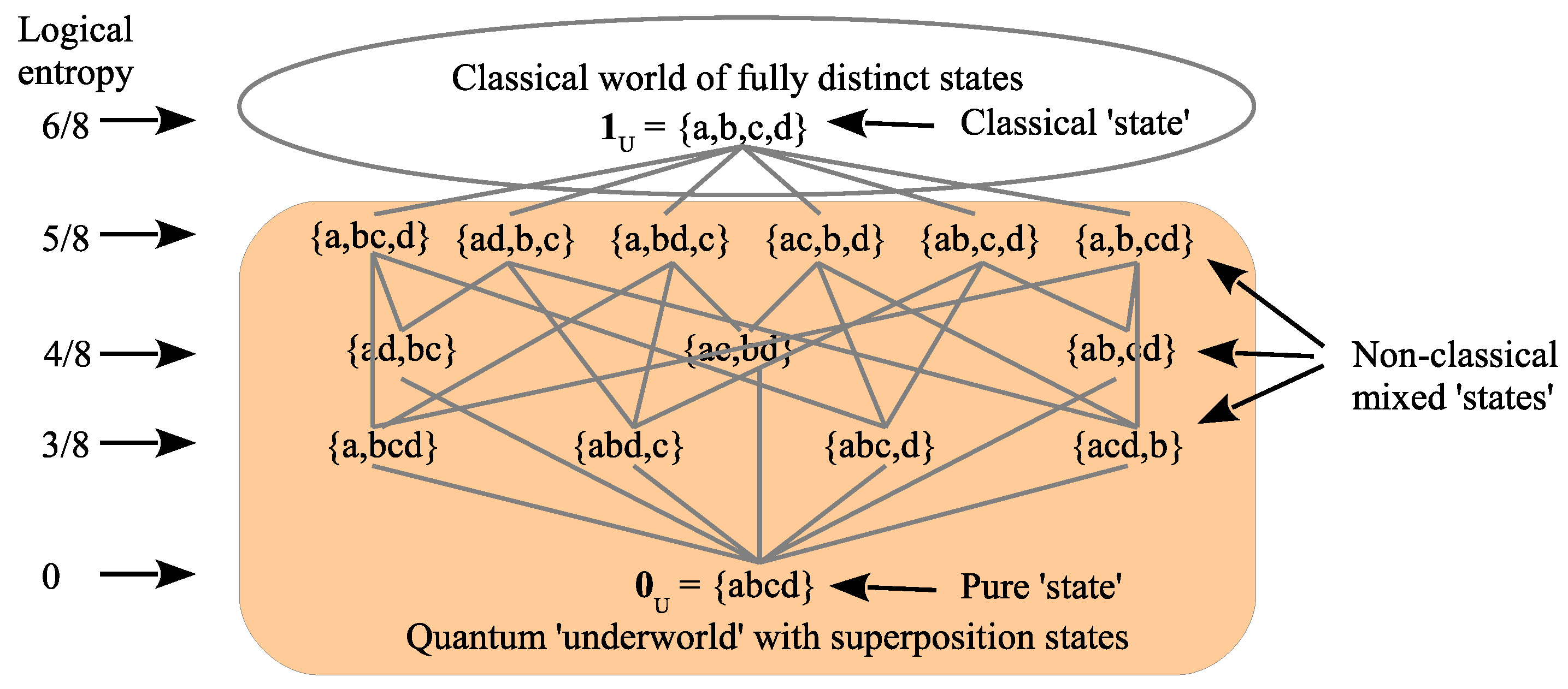
The simplified pedagogical model allows us to use the lattice of partitions to attach an intuitive image to the classical world of fully distinguished states and the quantum ‘underworld’ of indefinite states–as in Figure 14. This model uses the lattice of partitions on the four state universe $U=\left\{a,b,c,d\right\}$. The logical entropies are for the equiprobable case and show how logical entropy, as the measurement of information-as-distinctions, increases as more distinctions are made moving up in the lattice.

The fact that the model ‘works’ (as a pedagogical model) is corroboration for the thesis that the mathematical machinery of full QM is the Hilbert space version of the mathematics of partitions that is expressed in the model. That view of the quantum world as ‘Indefinite World’ (not ‘Wave World’) might be described as the objective indefiniteness interpretation of quantum mechanics.