Sums of Independent Circular Random Variables and Maximum Likelihood Circular Uniformity Tests Based on Nonnegative Trigonometric Sums Distributions

Abstract

The sum of independent circular uniformly distributed random variables is also circular uniformly distributed. In this study, it is shown that a family of circular distributions based on nonnegative trigonometric sums (NNTS) is also closed under summation. Given the flexibility of NNTS circular distributions to model multimodality and skewness, these are good candidates for use as alternative models to test for circular uniformity to detect different deviations from the null hypothesis of circular uniformity. The circular uniform distribution is a member of the NNTS family, but in the NNTS parameter space, it corresponds to a point on the boundary of the parameter space, implying that the regularity conditions are not satisfied when the parameters are estimated by using the maximum likelihood method. Two NNTS tests for circular uniformity were developed by considering the standardised maximum likelihood estimator and the generalised likelihood ratio. Given the nonregularity condition, the critical values of the proposed NNTS circular uniformity tests were obtained via simulation and interpolated for any sample size by the fitting of regression models. The validity of the proposed NNTS circular uniformity tests was evaluated by generating NNTS models close to the circular uniformity null hypothesis.

1. Introduction

A circular random variable takes values on the unit circle, and its density function must be periodic. Generally, a circular random variable represents an angle in the interval $(0,2\pi ]$, and it is important to model many random phenomena in different areas, such as in meteorology for the wind direction, in biology for the dihedral angles defining the spatial structure of a protein, in ecology for camera trap data that records the time of the day at which different animals are observed and in many other examples in other disciplines.

The circular distributions based on nonnegative trigonometric sums (NNTS) developed by ref. [1] are flexible distributions capable of modelling circular data that present multimodality and/or skewness (asymmetry). Fernández-Durán and Gregorio-Domínguez in [2] developed an efficient optimisation algorithm for manifolds to obtain maximum likelihood estimates of the parameters of an NNTS model. This algorithm was implemented by using the R package $CircNNTSR$ [3]. The NNTS family of distributions includes the uniform distribution as a special case (M = 0). One of the most important hypothesis tests in the study of circular statistics is testing for circular uniformity [4,5]. In addition, for absolutely continuous circular density functions, the circular uniform density is closed under summation, that is, the sum of independent circular uniformly distributed random variables has a circular uniform distribution [5]. Additionally, if at least one member of the sum of independent circular random variables is uniformly distributed, then the sum of these random variables is also circular uniformly distributed. This is a consequence of the characteristic function of a circular uniformly distributed random variable, ${\varphi }_{unif}\left(t\right)$, defined for $t\in \mathbb{R}$ as:

$${\varphi }_{unif}\left(t\right)=I(t=0)$$

(1)

where $I(t=0)$ is an indicator function that takes the value of one for $t=0$ and zero otherwise.

There are many different tests for circular uniformity, such as the Rayleigh test, Watson’s test, Kuiper’s test, and Rao’s spacing test, among others [6,7,8]. Many of these tests were designed with unimodal distributions as an alternative hypothesis and presented low power when applied to multimodal datasets. The Hermans-Rasson test, Bogdan test and Pycke test consider multimodal circular distributions as alternative hypotheses and have more power to detect deviations from circular uniformity when applied to multimodal circular data [9,10,11]. In this study, two tests are developed with alternative hypotheses NNTS distributions to account for the cases that present multimodality but also asymmetry. The NNTS tests are based on the maximum likelihood method: The first test is based on the standardised maximum likelihood estimator, and the second is based on the generalised likelihood ratio statistic. The power of the NNTS tests was compared to that of the Hermans-Rasson and Pycke tests. The results of the sums of NNTS random variables allow us to identify NNTS densities that are close to the uniform distribution, and we use these results to compare the power of the tests in simulated datasets where the degree of closeness to the circular uniform distribution can be controlled. This study is divided into seven sections, including the introduction. In the second section, mathematical formulas for the characteristic function of an NNTS circular random variable are developed. In the third section, the NNTS family is shown to be closed under summation; that is, the sum of independent NNTS circular random variables is also NNTS distributed, and how to obtain the parameters of the NNTS density of the sum and numerical examples with graphs is explained. In the fourth section, the two proposed circular uniformity tests, taking an NNTS distribution as an alternative hypothesis are developed. Considering the parameter space of NNTS densities, the null circular uniformity distribution corresponds to a parameter on the boundary of the parameter space. Then, the regularity conditions of maximum likelihood estimation are not satisfied because the parameters of the NNTS densities are estimated by maximum likelihood, and the critical values of the NNTS circular uniformity test are obtained by simulation. Ref. [12] showed the inconsistency of the bootstrap method when the parameter is on the boundary of the parameter space. Alternative bootstrap methods have been developed by Cavaliere, Nielsen and Rahbek to apply the bootstrap method when some or all the elements of the parameter vector are on the boundary of the parameter space [13,14]. They applied the proposed modified bootstrap method to the family of ARCH models for modelling the volatility of financial time series. These modified bootstrap methods require the simulation of bootstrap samples from the model in which the parameter estimates are specified with a shrinkage towards the boundary values at an appropriate rate. In this paper, since the null hypothesis with parameters on the boundary of the parameter space is completely specified, we considered a simpler approach in which we sampled from the null circular uniform distribution, calculated the test statistic and repeated this process for many null samples to estimate the critical values at significance levels of 10%, 5% and 1%. This procedure is repeated for samples of different sizes. The estimated critical values for different sample sizes are used in a regression model to obtain interpolated values of the critical values for any sample size, as suggested by Cuddington and Navidi [15]. Finally, we obtained a regression formula for the critical values for any sample size that satisfies the asymptotic values of the critical values of the test statistic observed for very large simulated samples sizes. In the fifth section, the power of the NNTS circular uniformity tests is examined by considering the results of the sums of the NNTS random variables in the third section to consider alternative circular distributions that are close to the null circular uniform distribution. The practical application of the proposed tests to real data on the time of occurrence of earthquakes and the flying orientation of home pigeons is presented in the sixth section. Finally, in the seventh section, conclusions are presented.

2. Characteristic Function of an NNTS Circular Random Variable

A circular random variable $\mathrm{\Theta }$ is defined as a random variable with unit circle support. These random variables are relevant when modelling seasonal patterns in many different scientific areas. Let $\mathrm{\Theta }$ be a circular random variable with an NNTS distribution with support interval $[0,2\pi )$ with a density function defined as the squared norm of a sum of complex trigonometric terms:

$$f_{\mathrm{\Theta }}\left(\theta \right)=\frac{1}{2\pi }{\left|\left|\sum _{k=0}^M{c}_k{e}^{ik\theta }\right|\right|}^2=\frac{1}{2\pi }\sum _{k=0}^M\sum _{m=0}^M{c}_k{\overline{c}}_m{e}^{i(k-m)\theta }$$

(2)

where $i=\sqrt{-1}$ and $e^{ik\theta }=cos\left(k\theta \right)+isin\left(k\theta \right)$. Complex parameter vector $\underline{c}=(c_0,c_1,\dots ,c_M)$ with complex numbers $c_k=c_{rk}+i{c}_{ik}$ and ${\overline{c}}_k=c_{rk}-i{c}_{ik}$, where $c_{rk}$ and $c_{ik}$ are the real and imaginary parts of the complex number $c_k$, respectively. The parameter vector $\underline{c}$ must satisfy ${\sum }_{k=0}^M\left|\right|c_k{\left|\right|}^2=1$ where $\left|\right|c_k{\left|\right|}^2=c_{rk}^2+c_{ik}^2$ is the squared norm of the complex number $c_k$. Given this parameter constraint, $c_0$ must be a positive real number related to the density concentration around its modes. The parameter set is a subset of the surface of a complex unit hypersphere in the space of complex numbers of dimension $M+1$, ${\mathbb{C}}^{M+1}$ because $\underline{c}$ and $-\underline{c}$ produce the same NNTS density. In addition, the vector of parameters $\underline{c}$ written in reverse order, produces the same NNTS density. For identifiability, we considered the parameter vectors $\underline{c}$ with $c_0$ positive and $c_0^2>\left|\right|c_{M+1}{\left|\right|}^2$. The number of terms in the sum M is an additional parameter that determines the maximum number of modes of the NNTS density function. By increasing M, it is possible to increase the number of modes and/or the concentration around the modes in the NNTS density function. The case $M=0$ corresponds to a circular uniform distribution, $f_{\mathrm{\Theta }}\left(\theta \right)=\frac{1}{2\pi }$. The NNTS density satisfies the periodicity constraint for a circular density $f\left(\theta \right)=f(\theta +(2\pi \left)r\right)$ for any integer r.

The characteristic function of a circular random variable, ${\varphi }_{\mathrm{\Theta }}\left(t\right)$, is defined as

$${\varphi }_{\mathrm{\Theta }}\left(t\right)=E\left(e^{it\theta }\right)={\int }_0^{2\pi }{e}^{it\theta }{f}_{\mathrm{\Theta }}\left(\theta \right)d\theta .$$

(3)

The characteristic function of an NNTS circular random variable is obtained as

$${\varphi }_{\mathrm{\Theta }}\left(t\right)=E\left(e^{it\theta }\right)={\int }_0^{2\pi }{e}^{it\theta }\frac{1}{2\pi }\sum _{k=0}^M\sum _{m=0}^M{c}_k{\overline{c}}_m{e}^{i(k-m)\theta }d\theta =\frac{1}{2\pi }\sum _{k=0}^M\sum _{m=0}^M{c}_k{\overline{c}}_m{\int }_0^{2\pi }{e}^{i(k-m+t)\theta }d\theta$$

(4)

then

$${\varphi }_{\mathrm{\Theta }}\left(t\right)=I(t=0)+\underset{k\ne m}{\sum _{k=0}^M\sum _{m=0}^M}{c}_k{\overline{c}}_{m}I(t=m-k)$$

(5)

where $I(t=a)$ is an indicator function that takes the value of one if $t=a$ and zero otherwise. This result is obtained because the integral ${\int }_0^{2\pi }{e}^{ir\theta }d\theta$ is zero for $r\ne 0$ and equal to $2\pi$ for $r=0$. Rearranging the terms in Equation (5), we obtain

$${\varphi }_{\mathrm{\Theta }}\left(t\right)=I(t=0)+\sum _{k=-M}^{-1}\left(\sum _{j=0}^{M-k}{c}_j{\overline{c}}_{j+k}\right)I(t=k)+\sum _{k=1}^M\left(\sum _{j=0}^{M-k}{c}_{j+k}{\overline{c}}_j\right)I(t=k).$$

(6)

Thus, the characteristic function of an NNTS circular random variable takes values on the integers $-M,-M+1,\dots ,-1,0,1,\dots ,M$, and these values are functions of the vector of parameters $\underline{c}={(c_0,c_1,\dots ,c_M)}^{\top }$.

3. Distribution of the Sum of Independent NNTS Circular Random Variables

Let ${\mathrm{\Theta }}_1,{\mathrm{\Theta }}_2,\dots ,{\mathrm{\Theta }}_S$ be independent NNTS circular random variables with parameter vectors ${\underline{c}}^{\left(1\right)}$, ${\underline{c}}^{\left(2\right)}$, …, ${\underline{c}}^{\left(S\right)}$ and $M_1, M_2, \dots , M_S$, respectively. For independent random variables, the characteristic function of ${\sum }_{k=1}^S{\mathrm{\Theta }}_k$, ${\varphi }_{{\sum }_{k=1}^S{\mathrm{\Theta }}_k}\left(t\right)$, satisfies

$${\varphi }_{{\sum }_{k=1}^S{\mathrm{\Theta }}_k}\left(t\right)=\prod _{k=1}^S{\varphi }_{{\mathrm{\Theta }}_k}\left(t\right).$$

(7)

In particular, for the case of two summands, $S=2$, ${\varphi }_{{\mathrm{\Theta }}_1+{\mathrm{\Theta }}_2}\left(t\right)={\varphi }_{{\mathrm{\Theta }}_1}\left(t\right){\varphi }_{{\mathrm{\Theta }}_2}\left(t\right)$ and for the NNTS case,

$$\begin{array}{ccc}\hfill {\varphi }_{{\mathrm{\Theta }}_1+{\mathrm{\Theta }}_2}\left(t\right)& =& \left(I(t=0)+\sum _{k=-M_1}^{-1}\left(\sum _{j=0}^{M_1-k}{c}_j^{\left(1\right)}{\overline{c}}_{j+k}^{\left(1\right)}\right)I(t=k)+\sum _{k=1}^{M_1}\left(\sum _{j=0}^{M_1-k}{c}_{j+k}^{\left(1\right)}{\overline{c}}_j^{\left(1\right)}\right)I(t=k)\right)\hfill \\ & \times & \left(I(t=0)+\sum _{k=-M_2}^{-1}\left(\sum _{j=0}^{M_2-k}{c}_j^{\left(2\right)}{\overline{c}}_{j+k}^{\left(2\right)}\right)I(t=k)+\sum _{k=1}^{M_2}\left(\sum _{j=0}^{M_2-k}{c}_{j+k}^{\left(2\right)}{\overline{c}}_j^{\left(2\right)}\right)I(t=k)\right).\hfill \end{array}$$

Finally, obtaining

$$\begin{array}{ccc}\hfill {\varphi }_{{\mathrm{\Theta }}_1+{\mathrm{\Theta }}_2}\left(t\right)& =& I(t=0)+\sum _{k=-min\{M_1,M2\}}^{-1}\left(\sum _{j=0}^{min\{M_1,M-2\}-k}{c}_j^{\left(1\right)}{\overline{c}}_{j+k}^{\left(1\right)}{c}_j^{\left(2\right)}{\overline{c}}_{j+k}^{\left(2\right)}\right)I(t=k)+\hfill \\ & & \sum _{k=1}^{min\{M_1,M_2\}}\left(\sum _{j=0}^{min\{M_1,M_2\}-k}{c}_{j+k}^{\left(1\right)}{\overline{c}}_j^{\left(1\right)}{c}_{j+k}^{\left(2\right)}{\overline{c}}_j^{\left(2\right)}\right)I(t=k).\hfill \end{array}$$

Extending this result to the case of S summands, the characteristic function of the sum ${\sum }_{k=1}^S{\mathrm{\Theta }}_k$ of the independent NNTS circular random variables is given by

$$\begin{array}{ccc}\hfill {\varphi }_{{\sum }_{k=1}^S{\mathrm{\Theta }}_k}\left(t\right)& =& I(t=0)+\hfill \\ & & \sum _{k=-min\{M_1,M2,\dots ,M_S\}}^{-1}\left(\sum _{j=0}^{min\{M_1,M-2,\dots ,M_S\}-k}\prod _{s=1}^S{c}_j^{\left(s\right)}{\overline{c}}_{j+k}^{\left(s\right)}\right)I(t=k)+\hfill \\ & & \sum _{k=1}^{min\{M_1,M_2,\dots ,M_S\}}\left(\sum _{j=0}^{min\{M_1,M_2,\dots ,M_S\}-k}\prod _{s=1}^S{c}_{j+k}^{\left(s\right)}{\overline{c}}_j^{\left(s\right)}\right)I(t=k).\hfill \end{array}$$

Thus, the NNTS family of circular distributions is closed under summation; that is, the sum of independent NNTS circular random variables is an NNTS circular random variable with parameter $M_{sum}=min\{M_1,M_2,\dots ,M_S\}$ and parameter ${\underline{c}}^{sum}$, which is a function of the vectors of parameters ${\underline{c}}^{\left(s\right)}$, $s=1,\dots ,S$.

To obtain the vector of parameters ${\underline{c}}^{sum}$, the following system of $M_{sum}$ equations involving the real parameter $c_0^{sum}$ is considered.

$$\prod _{s=1}^S{c}_k^{\left(s\right)}{\overline{c}}_0^{\left(s\right)}=c_0^{sum}{c}_k^{sum}$$

(8)

for $k=1,\dots ,M_{sum}$ and the norm equation

$${\left(c_0^{sum}\right)}^2+\sum _{k=1}^{M_{sum}}\left|\right|c_k^{sum}{\left|\right|}^2=1.$$

(9)

By considering the real and imaginary parts in Equations (8) and (9), this system of $2M_{sum}+1$ nonlinear real equations can be solved numerically. In particular, one can use the R package $rootSolve$ considering the vector with one in its first entry and zeroes in the other entries that correspond to the uniform distribution case as initial values [16].

For the sum of more than two NNTS circular random variables, the result for two random variables can be applied recursively.

3.1. Case $M=1$

If both summands are NNTS random variables with $M=1$, then the density function of their sum can be obtained analytically as follows: By considering the squared norm in the equations defined in Equation (8), we obtain

$$\left|\right|\prod _{s=1}^S{c}_k^{\left(s\right)}{\overline{c}}_0^{\left(s\right)}{\left|\right|}^2={\left(c_0^{sum}\right)}^2\left|\right|c_k^{sum}{\left|\right|}^2.$$

(10)

Substituting these equations into Equation (9), the following equation for $c_0^{sum}$ is obtained:

$${\left(c_0^{sum}\right)}^2+\sum _{k=1}^{M_{sum}}\frac{\left|\right|{\prod }_{s=1}^S{c}_k^{\left(s\right)}{\overline{c}}_0^{\left(s\right)}{\left|\right|}^2}{{\left(c_0^{sum}\right)}^2}=1$$

(11)

which is equivalent to the following biquadratic equation on $c_0^{sum}$:

$${\left(c_0^{sum}\right)}^4-{\left(c_0^{sum}\right)}^2+\sum _{k=1}^{M_{sum}}\left|\right|\prod _{s=1}^S{c}_k^{\left(s\right)}{\overline{c}}_0^{\left(s\right)}{\left|\right|}^2=0$$

(12)

with the largest positive solution given by

$$c_0^{sum}=\sqrt{\frac{1+\sqrt{1-4{\sum }_{k=1}^{M_{sum}}\left|\right|{\prod }_{s=1}^S{c}_k^{\left(s\right)}{\overline{c}}_0^{\left(s\right)}{\left|\right|}^2}}{2}}.$$

(13)

Once the value of $c_0^{sum}$ is determined, the values of $c_1^{sum},\dots ,c_{M_{sum}}^{sum}$ can be obtained by using the system of equations in Equation (8).

Thus, for the sum of two NNTS circular random variables with $M=$ 1, the c parameters are given by

$$c_0^{sum}=\sqrt{\frac{1+\sqrt{1-4\left|\right|c_1^{\left(1\right)}{\overline{c}}_0^{\left(1\right)}{c}_1^{\left(2\right)}{\overline{c}}_0^{\left(2\right)}{\left|\right|}^2}}{2}}$$

(14)

and

$$c_1^{sum}=\frac{c_0^{\left(1\right)}{c}_1^{\left(2\right)}{c}_0^{\left(2\right)}}{c_0^{sum}}.$$

(15)

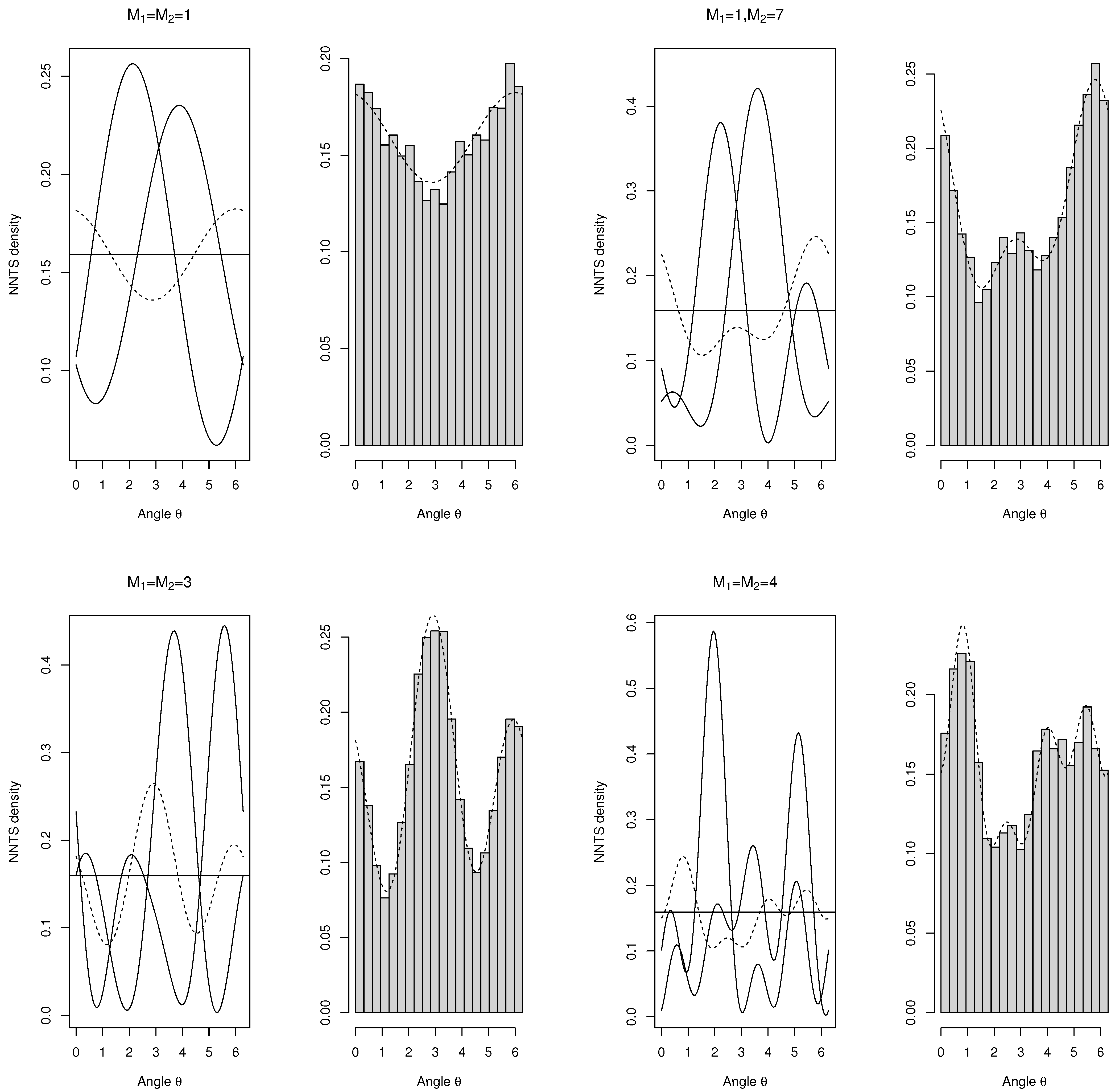
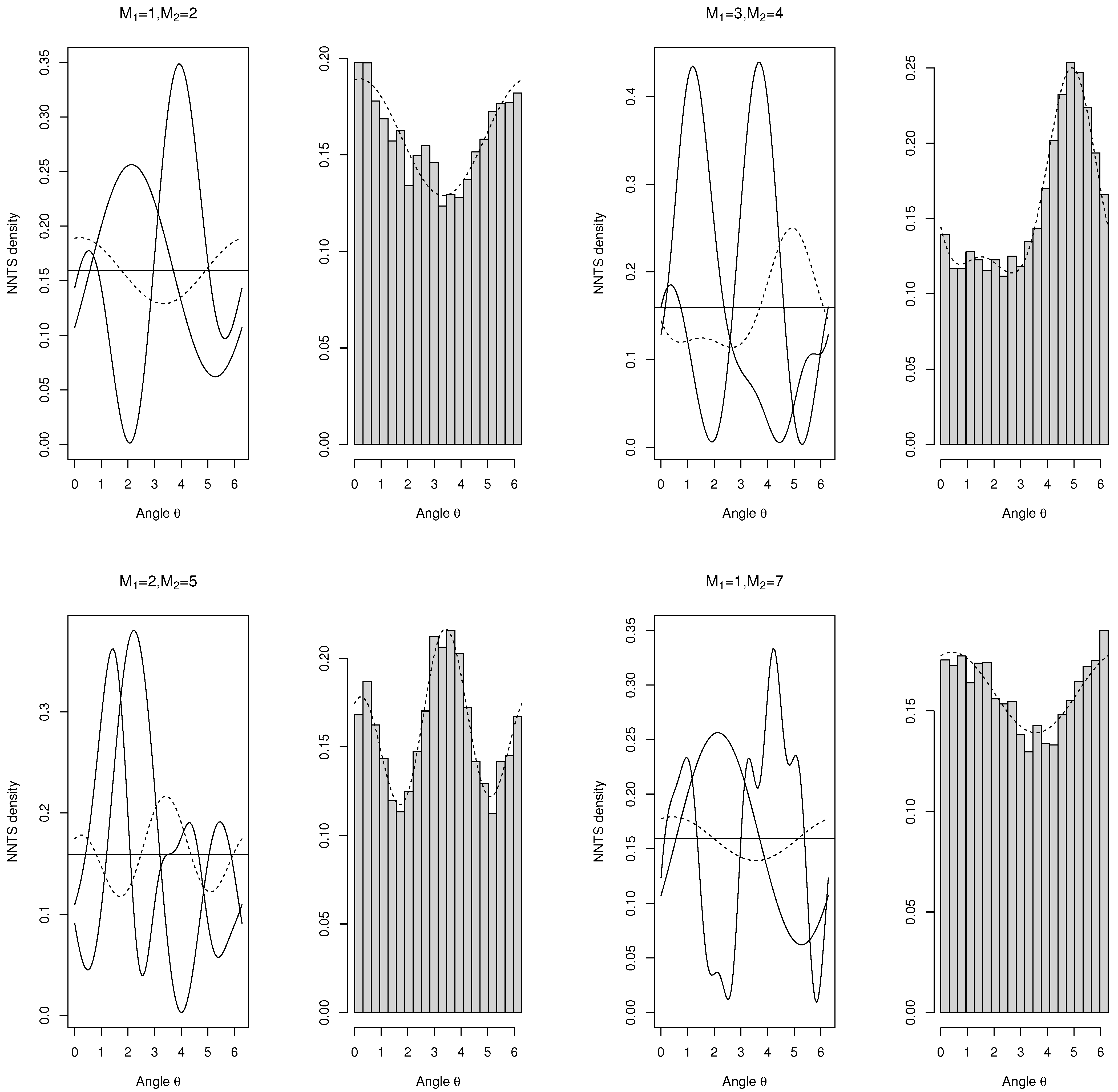
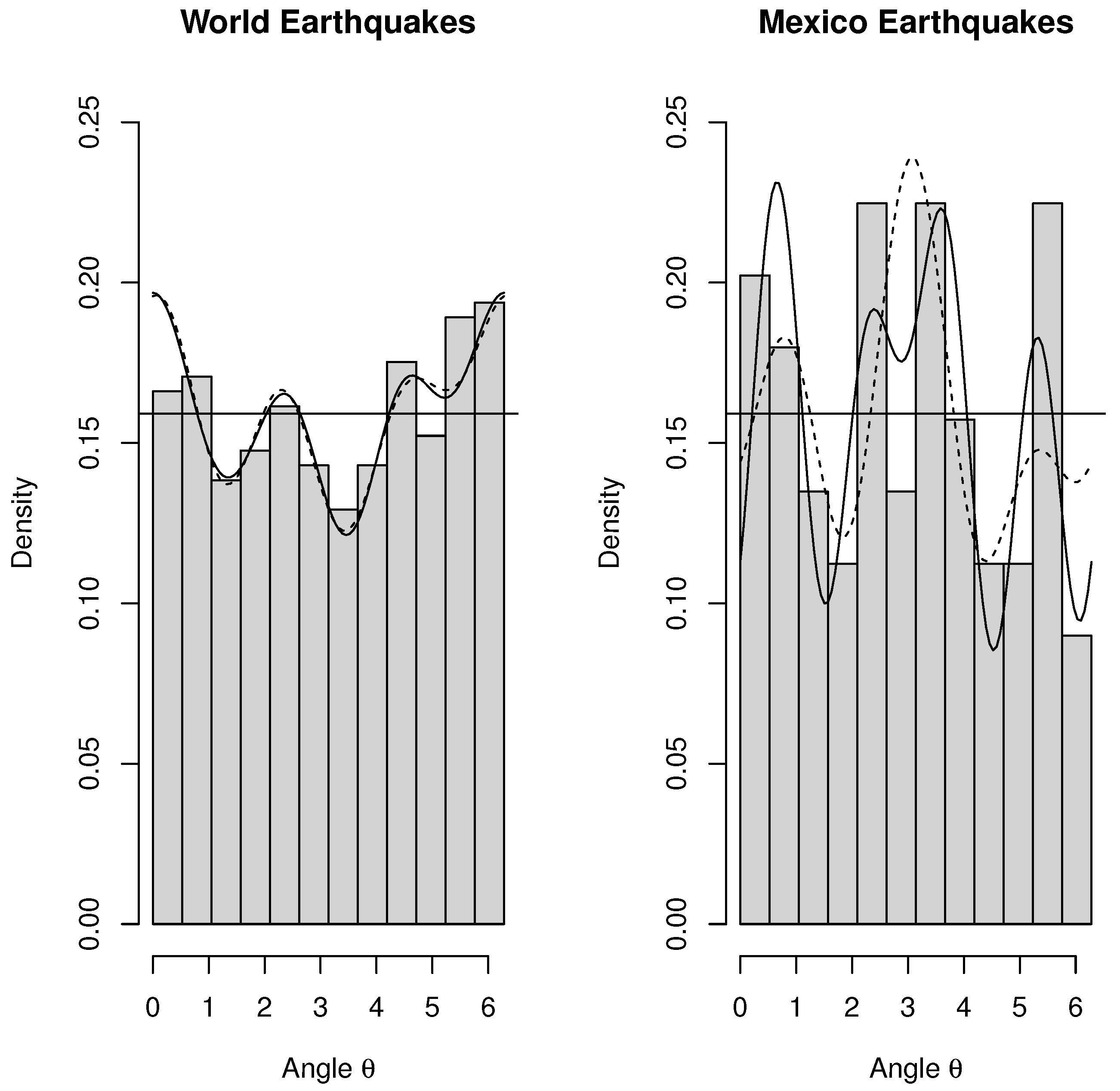
3.2. Numerical Examples

In the case of the sum of two NNTS circular random variables with different values of M, Figure 1 and Figure 2 show the density functions of the two random variables and their sum. In addition, the horizontal line corresponding to the circular uniform density ($M=0$) was included to appreciate the convergence of the sum to the circular uniform density. The plots on the right of Figure 1 and Figure 2 include the histograms of 1000 realisations from the sum of the two univariate NNTS densities; considering realisations from each of the summands and then their sum (modulus 2$\pi$), the NNTS density of the sum is superimposed on the histograms.

Figure 1. Examples of plots of the density functions of the sum of two NNTS elements with the same value of M for M = 1, 2, 3, and 4. The left plots show the plots of the NNTS densities of the variables in the sum and the NNTS density of the resulting sum. The right plots show the histograms of 1000 realisations from the resulting NNTS model of the sum superimposed with the NNTS density of the sum.

Figure 2. Examples of plots of the density functions of the sum of two NNTS elements with different values of M, $M_1$ and $M_2$, for the combinations $(M_1,M_2)$ = (1, 2), (3, 4), (2, 5), and (1, 7). The right plots show the histograms of 1000 realisations from the resulting NNTS model of the sum superimposed with the NNTS density of the sum.

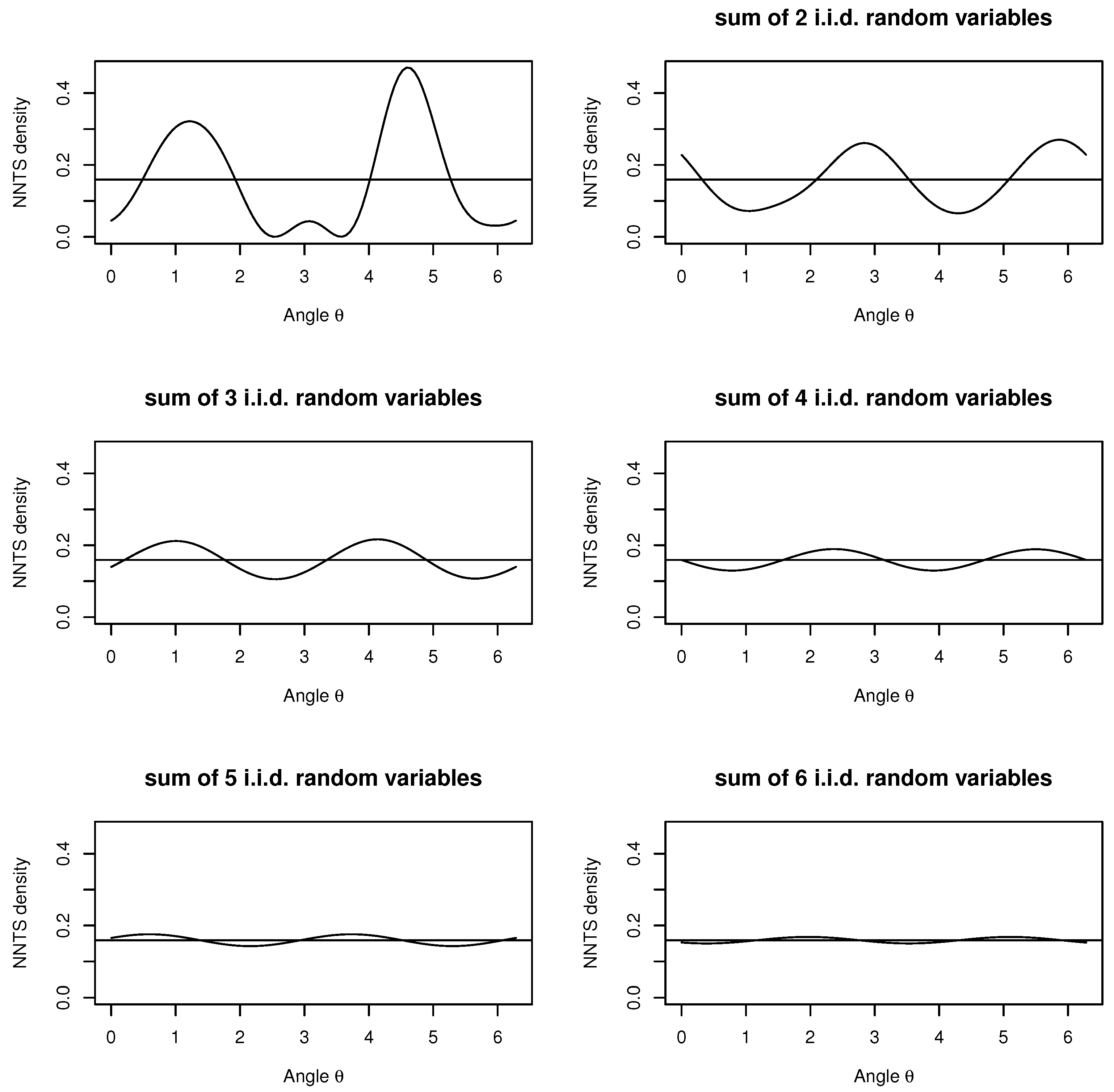
Figure 3 presents, for a simulated case with $M=5$, the plots of the NNTS densities for the case of independent and identically distributed random variables, in which we add recursively to obtain the density function of the sum of 2, 3, 4, 5, and 6 random variables. From Figure 3, it is clear how the convergence to the circular uniform distribution occurs very fast, with the sum of three or more random variables appearing almost circularly uniformly distributed.

Figure 3. Examples of plots of densities of sums of i.i.d. NNTS random variables with M = 5. The first plot shows the NNTS density with M = 5.

4. Two Circular Uniformity Tests with NNTS as Alternative Hypotheses

Many tests for circular uniformity have been reported in the literature. Among the most used in practice, one finds the Rayleigh test against a unimodal alternative, Kuiper’s test, Watson’s test, and the range test among many others [4,5,17]. As noted by Fisher, circular uniformity tests depend on the specification of the model in the alternative hypothesis, and one wants to have an alternative model that has a different number of modes to detect any departure from uniformity ([4], p. 65). Given that the family of NNTS circular distributions is nested, that is, all models with $M=M^{*}$ are particular cases of NNTS circular distributions with $M=M^{**}$ with $M^{**}>M^{*}$, NNTS circular distributions are suitable models for detecting any departure from uniformity for a sufficiently large sample size. Various studies have been conducted on the low power of many circular uniformity tests. For example, ref. [18] compared the power of the Rayleigh test, Watson’s test, Kuiper’s test, Rao’s spacing test, Bogdan test, and Hermans-Rasson test. Their main conclusions are that the Rayleigh test is preferred for unimodal departures from circular uniformity and that for multimodal departures from circular uniformity, the Hermans-Rasson test is recommended when considering mixtures of von Mises distributions as alternative models and eight different sample sizes (10, 15, 20, 25, 30, 40, 80, and 100). In the case of symmetric multimodality, the transformation of the data to a unimodal distribution and application of the Rayleigh test is recommended. Later, Landler et al. compared the power of the Rayleigh test, the Hermans-Rasson original test, a modification of the Hermans-Rasson test, and the Pycke test when considered as alternative model mixtures of von Mises distributions with modes equally distributed in the interval $[0,2\pi )$ with different proportions assigned to the different elements of the mixture and a sample size of 60 [19]. The final recommendations are to use the Rayleigh tests for unimodal departures from circular uniformity, the original Hermans-Rasson test for alternative distributions with at least two modes, and when the sample size is large and one considers at least two modes in the alternative distribution, the recommendation is to use the Pycke test instead. In addition, they point to the difficulty of testing for circular uniformity when the number of modes is greater than two and the alternative distribution is unknown and recommend substantially increasing the sample size and running the Pycke test with the constraint that the observed angles are supposed to show a high concentration around the modes. Given these results, we compared the power of the two proposed NNTS tests against four different tests: the Rayleigh test, the original and modified Hermans-Rasson tests, and the Pycke test. For a random sample of angles ${\theta }_1,{\theta }_2,\dots ,{\theta }_n$, the test statistic, as presented in [19], of the original Hermans-Rasson test is

$$T_{HRo}=\frac{n}{\pi }-\left(\frac{1}{2n}\right)\sum _{i=1}^n\sum _{j=1}^n|sin({\theta }_1-{\theta }_j)|,$$

(16)

the modified Hermans-Rasson test is

$$T_{HRm}=\left(\frac{1}{n}\right)\sum _{i=1}^n\sum _{j=1}^n\left(\left|\right|{\theta }_i-{\theta }_j|-\pi |-\frac{\pi }{2}-2.895\left(\right|sin({\theta }_i-{\theta }_j)|-\frac{2}{\pi })\right)$$

(17)

while the Pycke test is

$$T_P=\left(\frac{1}{n}\right)\sum _{i=1}^n\sum _{j=1}^n\left(\frac{2(cos({\theta }_i-{\theta }_j)-\sqrt{0.5})}{1.5-(2\sqrt{0.5}cos({\theta }_i-{\theta }_j))}\right).$$

(18)

The Hermans-Rasson tests belong to the family of circular uniformity tests of Beran, also known as Sobolev’s tests, in which the mean resultant length of the observations is p-fold wrapped on the unit circle, which is equivalent to considering the powers of the unit complex vectors with arguments given by the observed angles and calculating their mean resultant lengths, thereby obtaining weighted sums of Rayleigh statistics for different powers [5,20]. Like this study, ref. [11] considered multimodal alternative distributions that correspond to Fourier transformations that are equivalent to NNTS densities but Pycke did not consider the constraints in the parameter space to obtain a valid density function that is positive and integrates to one. Pycke found that the distribution of his test statistic is of a nonstandard form and corresponds to a weighted sum of chi-square distributions in which the weights are unknown complex functions of the observations [11]. Given the convergence of the distribution of the sum of circular random variables to the circular uniform distribution and, for the case of NNTS circular random variables, it is possible to investigate and compare the properties of the proposed NNTS test for cases where the parameter vector is close to the value specified to the null hypothesis. A circular uniformity test with NNTS distributions as alternative hypotheses exploits the flexibility of NNTS densities, which can model very different patterns for the alternative distribution in terms of the number of modes and asymmetry. For the NNTS test, the null and alternative hypotheses were specified as follows:

$$H_0:M=0 \mathrm{vs}. H_a:M=M^{*}>0.$$

(19)

or, equivalently,

$$H_0:f_{\mathrm{\Theta }}\left(\theta \right)=\frac{1}{2\pi } \mathrm{vs}. H_a:f_{\mathrm{\Theta }}\left(\theta \right)=\frac{1}{2\pi }{\left|\left|\sum _{k=0}^{M^{*}}{c}_k{e}^{ik\theta }\right|\right|}^2=\frac{1}{2\pi }\sum _{k=0}^{M^{*}}\sum _{m=0}^{M^{*}}{c}_k{\overline{c}}_m{e}^{i(k-m)\theta }.$$

(20)

In terms of the $\underline{c}$ parameter vector of an NNTS density with a fixed value of $M=M^{*}$, the null and alternative hypotheses are as follows:

$$H_0:\underline{c}={(1,0,0,\dots ,0)}^{\top } \mathrm{vs}. H_a:\underline{c}\ne {(1,0,0,\dots ,0)}^{\top }.$$

(21)

This hypothesis test is nonregular because the null hypothesis specifies the parameter vector on the boundary of the parameter space, and the maximum likelihood asymptotic results under regularity conditions do not apply. In particular, the likelihood ratio test statistic does not converge in distribution to a chi-squared distribution, and common bootstrap procedures are not applicable. Because the null hypothesis corresponds to the circular uniform distribution, the critical values of the NNTS test are obtained by simulating samples from the circular uniform distribution and, for each sample, fitting the NNTS model specified under the alternative hypothesis by maximum likelihood to calculate the value of the test statistic. For the first NNTS test for circular uniformity ($NNTS1$), we considered test statistic the standardised maximum likelihood estimator, $\widehat{\underline{c}}$, of the vector of parameters $\underline{c}$ defined as:

$$T_{NNTS1}={(\widehat{\underline{c}}-\underline{c})}^{H}j\left(\widehat{\underline{c}}\right)(\widehat{\underline{c}}-\underline{c})$$

(22)

where ${\underline{c}}^H$ is the Hermitian (conjugate and transpose) of the vector $\underline{c}$ and $j\left(\widehat{\underline{c}}\right)$ is the observed information that is proportional to the Hessian matrix that includes the second derivatives of the log-likelihood function, and for the NNTS density, it is equal to the projection matrix [2]

$$j\left(\widehat{\underline{c}}\right)=n(\mathbb{I}-\widehat{\underline{c}}{\widehat{\underline{c}}}^H)$$

(23)

where n is the sample size and $\mathbb{I}$ is the $(M+1)\times (M+1)$ identity matrix. Because $j\left(\widehat{\underline{c}}\right)$ is a projection matrix that is not an identity matrix, it is not invertible, making this a nonregular maximum likelihood estimation problem. Then,

$$T_{NNTS1}=n{(\widehat{\underline{c}}-{\underline{c}}_0)}^H(\mathbb{I}-\widehat{\underline{c}}{\widehat{\underline{c}}}^H)(\widehat{\underline{c}}-{\underline{c}}_0)=n{(\widehat{\underline{c}}-{\underline{c}}_0)}^H(\widehat{\underline{c}}-{\underline{c}}_0)-n{(\widehat{\underline{c}}-{\underline{c}}_0)}^H\left(\widehat{\underline{c}}{\widehat{\underline{c}}}^H\right)(\widehat{\underline{c}}-{\underline{c}}_0).$$

(24)

By partitioning the maximum likelihood estimator as ${\widehat{\underline{c}}}^H={({\widehat{c}}_0,{\widehat{c}}_1,\dots ,{\widehat{c}}_M)}^H={({\widehat{c}}_0,{\widehat{c}}_{1:M})}^H$ with ${\widehat{c}}_{1:M}^H={({\widehat{c}}_1,\dots ,{\widehat{c}}_M)}^H$ and considering that ${\sum }_{k=0}^M\left|\right|{\widehat{c}}_k{\left|\right|}^2=1$, one obtains ${(\widehat{\underline{c}}-{\underline{c}}_0)}^H(\widehat{\underline{c}}-{\underline{c}}_0)={({\widehat{c}}_0-1)}^2+1-{\widehat{c}}_0^2$ and ${(\widehat{\underline{c}}-{\underline{c}}_0)}^H\left(\widehat{\underline{c}}{\widehat{\underline{c}}}^H\right)(\widehat{\underline{c}}-{\underline{c}}_0)={(1-{\widehat{c}}_0)}^2$. Then,

$$T_{NNTS1}\left(\widehat{\underline{c}}\right)=n(1-{\widehat{c}}_0^2).$$

(25)

$T_{NNTS1}$ depends only on the first component of the maximum likelihood vector and, intuitively, because the sum of the norms of the components of the parameter vector, $\underline{c}$, should be equal to one, $T_{NNTS1}$ measures (scaled by the sample size) how far is ${\widehat{c}}_0^2$ of being equal to one that corresponds to the circular uniform distribution case.

Table 1 lists the critical values for $T_{NNTS1}$ obtained by the simulation for significance levels of 10%, 5%, and 1% for different sample sizes. We used a total of 10,000 simulated samples to obtain critical values. Given the recommendations in [15] for the number of simulated samples to produce critical values, the critical values in Table 1 and Table 2 are reported with a precision of 0.1.

Table 1. Critical values for significance levels of 10%, 5%, and 1% and sample sizes of 25, 50, 100, 200, and 500 for the NNTS circular uniformity test based on the standardised maximum likelihood estimator ($NNTS1$) with test statistic $T_{NNTS1}$. The critical values were obtained from 10,000 simulations from the null circular uniform distribution. For each simulated dataset, the alternative NNTS model is fitted, and the test statistic is calculated.

		Sample Size
$\mathit{M}$	$\mathit{\alpha }$	25	50	100	200	500
1	0.10	2.7	2.5	2.4	2.3	2.3
	0.05	3.7	3.3	3.1	3.1	3.1
	0.01	8.0	5.3	4.8	4.8	4.7
2	0.10	8.6	4.6	4.3	4.1	3.9
	0.05	9.2	5.9	5.2	5.0	4.9
	0.01	10.7	10.1	7.6	7.2	6.8
3	0.10		7.9	6.1	5.6	5.4
	0.05		13.1	7.3	6.7	6.4
	0.01		15.4	10.1	9.0	8.7
4	0.10		12.5	7.9	7.3	6.8
	0.05		13.9	9.6	8.4	7.9
	0.01		18.1	15.0	11.3	10.4
5	0.10			10.1	8.6	8.2
	0.05			13.0	10.0	9.4
	0.01			20.9	13.4	12.1

Table 2. Critical values for significance levels of 10%, 5%, and 1% and different sample sizes for the NNTS circular uniformity test based on the generalised likelihood ratio ($NNTS2$) with test statistic $T_{NNTS2}$. The critical values were obtained from 10,000 simulations from the null circular uniform distribution. For each simulated dataset, the alternative NNTS model is fitted, and the test statistic is calculated.

		Sample Size
$\mathit{M}$	$\mathit{\alpha }$	20	30	40	50	60	70	80	90	100	110	120	130	140	150	200	300	400	500	600	700	∞
1	0.10	5.0	4.9	4.9	4.7	4.7	4.7	4.6	4.6	4.6												4.6
	0.05	6.6	6.3	6.3	6.1	6.1	6.1	6.1	6.1	6.1												6.1
	0.01	10.3	9.8	9.8	9.5	9.5	9.4	9.4	9.3	9.3												9.3
2	0.10		8.5	8.3	8.1	8.1	8.0	8.0	8.0	7.9	7.9											7.9
	0.05		10.5	10.2	9.9	9.8	9.8	9.7	9.7	9.7	9.7											9.7
	0.01		14.5	14.3	14.0	13.8	13.7	13.7	13.6	13.5	13.5											13.5
3	0.10			11.6	11.3	11.2	11.1	11.0	11.0	10.9	10.9	10.9	10.8	10.8	10.8	10.8	10.8					10.8
	0.05			13.7	13.5	13.2	13.1	13.1	13.0	12.9	12.9	12.9	12.8	12.8	12.8	12.8	12.8					12.8
	0.01			17.9	17.9	17.9	17.6	17.5	17.4	17.3	17.3	17.3	17.2	17.1	17.1	17.0	17.0					17.0
4	0.10				14.5	14.2	14.1	13.9	13.9	13.8	13.7	13.7	13.7	13.7	13.6	13.6	13.5	13.5				13.5
	0.05				16.7	16.6	16.4	16.3	16.1	16.0	15.9	15.9	15.9	15.8	15.8	15.8	15.7	15.7				15.7
	0.01				21.4	21.4	21.3	20.9	20.9	20.8	20.8	20.7	20.6	20.5	20.5	20.3	20.3	20.3				20.3
5	0.10					17.3	17.1	16.9	16.8	16.7	16.6	16.5	16.5	16.4	16.3	16.3	16.2	16.1	16.1			16.1
	0.05					19.7	19.6	19.5	19.2	19.1	19.0	18.9	18.9	18.8	18.7	18.6	18.6	18.5	18.5			18.5
	0.01					24.6	24.6	24.5	24.4	24.3	24.2	24.0	24.0	23.8	23.6	23.6	23.5	23.4	23.4			23.4
6	0.10						20.0	19.9	19.7	19.5	19.4	19.3	19.2	19.1	19.1	18.9	18.8	18.7	18.7	18.7		18.7
	0.05						22.6	22.4	22.4	22.1	22.0	21.9	21.9	21.8	21.7	21.5	21.3	21.2	21.2	21.2		21.2
	0.01						27.9	27.8	27.8	27.6	27.6	27.3	27.3	27.1	27.1	26.7	26.6	26.5	26.5	26.5		26.5
7	0.10							22.7	22.6	22.4	22.2	22.1	22.0	21.9	21.9	21.6	21.4	21.2	21.2	21.2	21.2	21.2
	0.05							25.4	25.4	25.1	25.0	24.9	24.9	24.7	24.6	24.3	24.1	24.0	24.0	23.9	23.9	23.9
	0.01							31.0	31.0	30.9	30.8	30.6	30.6	30.5	30.5	29.9	29.8	29.6	29.6	29.6	29.6	29.6

The second maximum likelihood NNTS test for circular uniformity is based on the generalised likelihood ratio statistic defined as

$$T_{NNTS2}=-2ln\left(\frac{{\widehat{L}}_{H_0}}{{\widehat{L}}_{H_a}}\right)=-2ln\left(\frac{{\widehat{L}}_{M=0}}{{\widehat{L}}_{M=M^{*}}}\right)=2ln\left({\widehat{L}}_{M=M^{*}}\right)+2nln\left(2\pi \right)$$

(26)

where ${\widehat{L}}_{M=M^{*}}$ is the maximised likelihood under the alternative hypothesis $H_a:M=M^{*}$, which corresponds to the maximised likelihood of the NNTS model with $M=M^{*}>0$. Again, because the maximum likelihood of the NNTS model does not satisfy the regularity conditions under the null hypothesis of uniformity, the critical values are obtained by simulation and are included in Table 2 for various values of M (1, 2, …, 7), significance levels $\alpha$ (10%, 5%, and 1%), and various sample sizes. Again, given the nonregular maximum likelihood estimation for NNTS models under the null hypothesis ($M=0$), the statistic $T_{NNTS2}$ does not converge to a chi-squared distribution for large sample sizes, and commonly used bootstrap procedures are not applicable. Table 2 contains a larger number of sample sizes than Table 1 since, as shown later in the paper, the NNTS2 has more power than the NNTS1 test and is recommended for use in practice. Running in parallel for different simulated samples in different cores of the processor, ten thousand simulated datasets are used to estimate the critical values of the $NNTS2$ statistic took, for sample sizes of 500, from approximately 38 min for $M=1$ to approximately 68 min for $M=5$ in an 8 core CPU at a speed of 3 GHz.

Following MacKinnon, Table 3 includes the fitted regression models to interpolate the critical values for any sample size with a precision of 0.1 (one decimal place) [21,22]. In this case, the regression models for the critical values considered as explanatory variables the reciprocal of the sample size and the NNTS parameter M and their interaction and the reciprocal of the squared sample size. The interaction between the squared sample size and M was not significant for all the considered models. Initially, a single regression model for all the values of M was considered, but for the cases $M=$ 1 and $M=$ 2, it did not present a good fit. Then, two separate regression models were fitted for the cases $M=$ 1 and $M=$ 2, in which only the sample size and M had significant coefficients. For the other considered values of M, 3 to 7, a common regression model was sufficient. As shown in Table 3, the fitted regression models had a good fit since their coefficients of determination are very high and their maximum absolute and relative errors are quite small. The relative errors are less than 2.1% for the model with $M=$ 1 and less than 1.3% for the other models ($M\ge 2$). Given these results, the critical values for all sample sizes can be interpolated for any sample size by using the fitted regression models. Given the observed precision of the regression models, in the case of an observed NNTS2 statistic, $T_{NNTS2}$, with a value that differs from the interpolated critical value by less than 0.1, the test can be considered inconclusive. Table 3 also includes the sample sizes at which the interpolated critical values by regression reach the asymptotic critical values observed in the simulations in Table 2. From these identified sample sizes, the asymptotic values obtained in the simulation are used in the implementation of the test. These asymptotic critical values were determined in the simulations by identifying many consecutive sample sizes at which the critical values obtained by simulation did not change. For the fitting of the regression models, we considered only the first two consecutive sample sizes at which the critical values did not change. From the simulations and by considering the critical values as a decreasing function of the sample size, the minimum sample size to apply the NNTS2 test for $M\ge$ 3 was found to be $10(M+1)$ which implies that we have at least 5 observations for each of the 2M NNTS parameters to be estimated. For cases $M=$ 1 and $M=$ 2, we found that the required minimum sample sizes are 15 and 25, respectively.

Table 3. Fitted regression models for the critical values in Table 2 to interpolate critical values of the generalised likelihood ratio test (NNTS2) for any sample size in terms of the reciprocal of the sample size ($SS$), the NNTS parameter M and their interaction and, the reciprocal of the squared sample size. The predictions of the regression models must be rounded to one decimal (precision 0.1). The minimum sample size for which the critical values are valid ($S{S}_{min}$) and the sample size at which the asymptotic critical values are reached ($S{S}_{asymptotic}$) are included. Also, the coefficient of determination ($R^2$) of the regression models and the maximum absolute and relative errors of the predicted critical values for the sample sizes in Table 2 are presented.

				Regression Models Estimated Coefficients						Abs.	Rel.
$\mathit{M}$	${\mathit{SS}}_{\mathit{min}}$	${\mathit{SS}}_{\mathit{asymptotic}}$	$\mathit{\alpha }$	Intercept	$\mathit{M}$	$\frac{\mathbf{1}}{\mathit{SS}}$	$\mathit{M}\left(\frac{\mathbf{1}}{\mathit{SS}}\right)$	${\left(\frac{\mathbf{1}}{\mathit{SS}}\right)}^{\mathbf{2}}$	${\mathit{R}}^{\mathbf{2}}$	Error	Error
1	15	85	0.10	4.5128		10.8062			0.8737	0.1	2.04%
			0.05	5.9269		12.7461			0.9229	0.1	1.59%
			0.01	9.0630		24.5377			0.9670	0.1	1.05%
2	25	98	0.10	7.6807		24.1698			0.9714	0.1	1.25%
			0.05	9.3118		34.1750			0.9539	0.1	1.03%
			0.01	13.1063		43.7094			0.9791	0.1	0.70%
3 to 7			0.10	3.2703	2.5317	−108.3235	32.8331	1618.5535	0.9999	0.1	0.93%
			0.05	4.6077	2.7291	−91.8270	31.8820	1368.6187	0.9997	0.2	1.03%
			0.01	7.2135	3.1555	26.9335	21.0319	−1549.4894	0.9995	0.2	1.12%
3	40	173
4	50	203
5	60	278
6	70	386
7	80	562

5. Power and Size Comparisons

We compared the Rayleigh (RT), modified Hermans-Rasson (HRmT), Pycke (PT), and NNTS ($NNTS1$ and $NNTS2$) tests in terms of their power and size by simulating samples from the null circular uniform distribution and the alternative NNTS distribution for sample sizes (SS) of 25, 50, 100, 200, and 500. We compared the power of the tests for significance levels $\alpha$ of 10%, 5%, and 1%. The R package $circular$ was used to calculate the test statistic of the Rayleigh test [23]. The Hermans-Rasson and Pycke tests were performed by using the R package $CircMLE$ [19,24]. Finally, for the $NNTS1$ and $NNTS2$ the R package $CircNNTSR$ was used [3]. To speed up the calculation of the NNTS tests, the computations were implemented in parallel by using the R package $parallel$ in an 8 core CPU at a speed of 3 GHz [25].

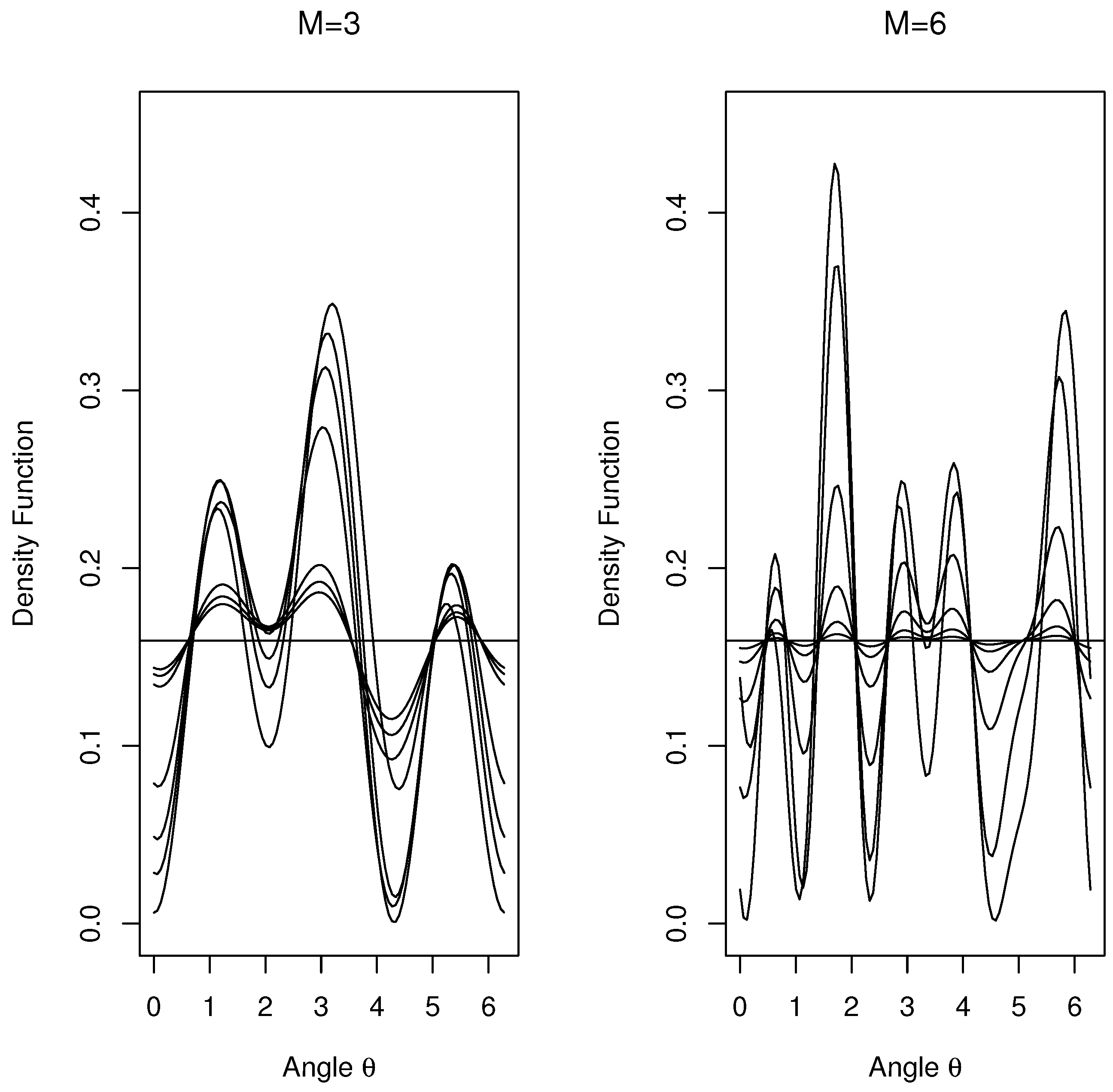
Figure 4 shows plots of the two NNTS alternative models with $M=3$ and $M=6$. For each of the two NNTS alternative models, we considered various values of the parameter $c_0$ to obtain alternative models that are close to the null circular uniform distribution. As shown in Figure 4, by increasing the value of parameter $c_0$, we obtain distributions that are closer to the circular uniform distribution. In terms of size, when simulating samples from the null circular uniform distribution and applying the tests, all the considered tests obtained an adequate observed frequency of rejection of the null hypothesis that was practically identical to the significance level. We used 1000 simulated samples from the null and alternative models in our simulations, and the frequencies corresponding to the observed power are reported in rounded percentages ranging from 0% to 100%.

Figure 4. Cases used for the power and size study for NNTS densities with $M=3$ (left) and $M=6$ (right). Note the convergence to the circular uniform distribution as $c_0$ approaches one.

Table 4, Table 5 and Table 6 contain the results for the power of the tests by using the observed frequencies, in percentage, for rejecting the null hypothesis of circular uniformity when simulating random samples from the alternative model with $M=3$ with eight different values of parameter $c_0$. The considered eight cases of the $c_0$ parameter range from 0.59 to 0.9959, with $c_0$ values near one representing densities closer to the circular uniform distribution, as shown in the left plot in Figure 4. Basically, in all cases and sample sizes where the power takes an acceptable value, the Hermans-Rasson (HRmT) test presented lower power than that for the Pycke (PT) test, and we then compared the NNTS ($NNTS1$ and $NNTS2$) tests against the Pycke (PT) test. For the sample size of 25, the Pycke test has the largest power, although it is below 0.6. For cases 1 to 5 and sample sizes of 25 and 50, the $NNTS2$ with $M=3$ had the largest power, followed by the $NNTS2$ test with $M=4$, which was followed by the Pycke test. In many cases and sample sizes, the $NNTS2$ test with $M=5$ has a very similar power to the Pycke test. This implies that when applying the generalised likelihood ratio $NNTS2$ test, there is some flexibility in the selection of the M value to be used in the test; in case of doubt between $M=M^{*}$ and $M=M^{*}+1$, it is recommended using $M=M^{*}+1$ to avoid a situation in which a smaller M is used and the power decreases considerably, as shown for the power values for the $NNTS2$ test with $M=2$ or $M=1$. For the largest sample sizes of 200 and 500 in Table 5 and Table 6, $NNTS1$ and $NNTS2$ present similar power values, showing that the two tests are equivalent for large sample sizes and significance levels of 5% and 1%, respectively. This convergence was achieved earlier for sample sizes of 100, 200, and 500 for a significance level of 10%, as shown in Table 4.

Table 4. Power comparison of the $NNTS1$ with $M=1,2,3,4, \mathrm{and} 5$, $NNTS2$ with $M=1,2,3,4, \mathrm{and} 5$, Rayleigh test ($RT$), modified Hermans-Rasson ($HRmT$), and Pycke ($PT$) tests considering a significance level $\alpha =10\%$. The power of the tests is obtained from the simulation of 1000 datasets from an NNTS density with $M=3$ (see left plot in Figure 4), applying the various tests to each of the datasets and, calculating the frequency at which the null hypothesis of circular uniformity is rejected. Underlined numbers are examples for which the $NNTS1$ or $NNTS2$ power is greater than the Pycke power by at least 3 (3%).

				$\mathit{NNTS}1$ Std. Max. Lik. Est.					$\mathit{NNTS}2$ Likelihood Ratio
Case	SS	${\mathit{c}}_{\mathbf{0}}$	$\mathbf{1}-{\mathit{c}}_{\mathbf{0}}^{\mathbf{2}}$	1	2	3	4	5	1	2	3	4	5	BIC	RT	HRmT	PT
1	25	0.59	0.6519	46	33				46	35				49	46	41	56
2	25	0.67	0.5511	37	30				39	32				44	41	37	55
3	25	0.75	0.4375	30	35				33	33				39	36	37	55
4	25	0.83	0.3111	29	38				33	37				42	36	37	53
5	25	0.91	0.1719	28	34				30	32				38	30	30	40
6	25	0.9899	0.0201	14	13				13	15				18	15	15	16
7	25	0.9939	0.0122	12	13				12	13				16	12	11	12
8	25	0.9959	0.0082	10	11				10	11				14	11	11	11
1	50	0.59	0.6519	71	63	92	85		72	61	95	92		86	71	67	89
2	50	0.67	0.5511	64	57	92	87		65	58	95	93		84	67	67	89
3	50	0.75	0.4375	55	62	91	85		59	56	96	93		82	63	63	88
4	50	0.83	0.3111	50	72	95	90		53	63	96	93		82	57	64	87
5	50	0.91	0.1719	43	67	83	75		46	59	86	80		71	47	55	70
6	50	0.9899	0.0201	17	19	17	17		18	19	20	18		23	18	18	19
7	50	0.9939	0.0122	12	14	15	16		12	14	17	17		16	12	14	16
8	50	0.9959	0.0082	12	13	13	13		12	12	14	13		15	12	11	12
1	100	0.59	0.6519	96	90	100	100	100	96	90	100	100	100	100	95	95	100
2	100	0.67	0.5511	90	84	100	100	100	91	84	100	100	100	98	91	93	100
3	100	0.75	0.4375	87	88	100	100	100	89	86	100	100	100	99	90	93	100
4	100	0.83	0.3111	83	95	100	100	100	86	92	100	100	100	99	87	94	100
5	100	0.91	0.1719	74	93	100	99	99	76	89	100	99	99	95	78	90	98
6	100	0.9899	0.0201	25	29	35	32	28	25	28	35	33	31	29	24	27	31
7	100	0.9939	0.0122	20	21	24	21	21	20	20	24	21	22	22	19	21	23
8	100	0.9959	0.0082	17	19	20	19	18	17	19	21	21	18	21	17	19	20
1	200	0.59	0.6519	100	100	100	100	100	100	100	100	100	100	100	100	100	100
2	200	0.67	0.5511	99	99	100	100	100	100	99	100	100	100	100	100	100	100
3	200	0.75	0.4375	100	99	100	100	100	100	99	100	100	100	100	100	100	100
4	200	0.83	0.3111	98	100	100	100	100	99	100	100	100	100	100	99	100	100
5	200	0.91	0.1719	95	100	100	100	100	95	99	100	100	100	100	95	100	100
6	200	0.9899	0.0201	40	50	63	57	55	41	47	62	57	53	45	40	48	57
7	200	0.9939	0.0122	31	34	43	37	37	31	33	43	37	36	34	30	33	39
8	200	0.9959	0.0082	24	28	32	28	27	23	27	31	29	27	25	23	26	29
1	500	0.59	0.6519	100	100	100	100	100	100	100	100	100	100	100	100	100	100
2	500	0.67	0.5511	100	100	100	100	100	100	100	100	100	100	100	100	100	100
3	500	0.75	0.4375	100	100	100	100	100	100	100	100	100	100	100	100	100	100
4	500	0.83	0.3111	100	100	100	100	100	100	100	100	100	100	100	100	100	100
5	500	0.91	0.1719	100	100	100	100	100	100	100	100	100	100	100	100	100	100
6	500	0.9899	0.0201	76	87	97	96	94	75	84	97	96	94	80	74	87	95
7	500	0.9939	0.0122	54	66	82	79	75	53	65	82	78	74	57	53	65	76
8	500	0.9959	0.0082	45	54	68	63	58	46	52	67	62	57	48	46	52	61

Table 5. Power comparison of the $NNTS1$ with $M=1,2,3,4, \mathrm{and} 5$, $NNTS2$ with $M=1,2,3,4, \mathrm{and} 5$, Rayleigh test ($RT$), modified Hermans-Rasson ($HRmT$), and Pycke ($PT$) tests considering a significance level $\alpha =5\%$. The power of the tests is obtained from the simulation of 1000 datasets from an NNTS density with $M=3$ (see left plot in Figure 4), applying the various tests to each of the datasets and, calculating the frequency at which the null hypothesis of circular uniformity is rejected. Underlined numbers are examples for which the $NNTS1$ or $NNTS2$ power is greater than the Pycke power by at least 3 (3%).

				$\mathit{NNTS}\mathbf{1}$ Std. Max. Lik. Est.					$\mathit{NNTS}\mathbf{2}$ Likelihood Ratio
Case	SS	${\mathit{c}}_{\mathbf{0}}$	$\mathbf{1}-{\mathit{c}}_{\mathbf{0}}^{\mathbf{2}}$	1	2	3	4	5	1	2	3	4	5	BIC	RT	HRmT	PT
1	25	0.59	0.6519	32	24				33	21				35	32	28	43
2	25	0.67	0.5511	25	24				27	21				29	30	25	41
3	25	0.75	0.4375	20	26				22	23				28	24	26	40
4	25	0.83	0.3111	18	27				22	24				29	25	26	37
5	25	0.91	0.1719	17	23				18	19				24	19	19	27
6	25	0.9899	0.0201	8	8				8	9				10	8	9	9
7	25	0.9939	0.0122	6	7				6	6				9	6	5	6
8	25	0.9959	0.0082	5	5				5	5				7	5	5	6
1	50	0.59	0.6519	58	50	80	76		59	49	89	85		79	58	56	80
2	50	0.67	0.5511	50	46	76	78		54	45	92	88		78	55	53	80
3	50	0.75	0.4375	40	48	76	77		46	44	91	86		74	49	50	79
4	50	0.83	0.3111	35	60	84	80		40	50	91	87		76	43	50	76
5	50	0.91	0.1719	30	56	69	61		31	47	75	68		60	34	40	57
6	50	0.9899	0.0201	10	11	10	10		9	11	11	10		14	9	10	11
7	50	0.9939	0.0122	7	8	9	9		6	6	9	9		10	6	6	8
8	50	0.9959	0.0082	6	8	7	6		6	7	7	7		9	6	6	7
1	100	0.59	0.6519	92	83	100	100	99	92	84	100	100	100	99	91	92	100
2	100	0.67	0.5511	83	75	100	100	98	85	76	100	100	100	97	84	86	100
3	100	0.75	0.4375	76	82	100	100	99	81	79	100	100	100	98	83	87	99
4	100	0.83	0.3111	71	91	100	100	100	76	85	100	100	100	99	79	88	99
5	100	0.91	0.1719	63	89	99	98	95	66	83	99	99	97	93	67	82	96
6	100	0.9899	0.0201	15	18	23	20	13	16	17	24	20	20	19	16	16	19
7	100	0.9939	0.0122	12	12	14	12	11	12	11	15	12	14	14	12	12	13
8	100	0.9959	0.0082	11	13	13	11	7	10	12	14	11	11	14	11	12	12
1	200	0.59	0.6519	100	99	100	100	100	100	99	100	100	100	100	100	100	100
2	200	0.67	0.5511	98	98	100	100	100	99	98	100	100	100	100	99	100	100
3	200	0.75	0.4375	98	99	100	100	100	98	99	100	100	100	100	99	100	100
4	200	0.83	0.3111	96	100	100	100	100	97	99	100	100	100	100	97	100	100
5	200	0.91	0.1719	90	100	100	100	100	91	98	100	100	100	100	91	99	100
6	200	0.9899	0.0201	27	37	50	44	41	27	35	50	44	40	32	27	34	43
7	200	0.9939	0.0122	19	24	30	26	25	19	23	29	26	24	26	19	22	25
8	200	0.9959	0.0082	15	19	21	18	17	15	18	20	18	17	16	15	16	19
1	500	0.59	0.6519	100	100	100	100	100	100	100	100	100	100	100	100	100	100
2	500	0.67	0.5511	100	100	100	100	100	100	100	100	100	100	100	100	100	100
3	500	0.75	0.4375	100	100	100	100	100	100	100	100	100	100	100	100	100	100
4	500	0.83	0.3111	100	100	100	100	100	100	100	100	100	100	100	100	100	100
5	500	0.91	0.1719	100	100	100	100	100	100	100	100	100	100	100	100	100	100
6	500	0.9899	0.0201	64	79	95	92	88	63	76	95	92	87	71	63	77	90
7	500	0.9939	0.0122	41	56	73	70	64	41	53	72	69	64	45	41	54	66
8	500	0.9959	0.0082	32	39	55	50	45	32	37	55	50	44	35	32	38	47

Table 6. Power comparison of the $NNTS1$ with $M=1,2,3,4, \mathrm{and} 5$, $NNTS2$ with $M=1,2,3,4, \mathrm{and} 5$, Rayleigh test ($RT$), modified Hermans-Rasson ($HRmT$), and Pycke ($PT$) tests considering a significance level $\alpha =1\%$. The power of the tests are obtained from the simulation of 1000 datasets from an NNTS density with $M=3$ (see left plot in Figure 4), applying the various tests to each of the datasets and, calculating the frequency at which the null hypothesis of circular uniformity is rejected. Underlined numbers are examples for which the $NNTS1$ or $NNTS2$ power is greater than the Pycke power by at least 3 (3%).

				$\mathit{NNTS}\mathbf{1}$ Std. Max. Lik. Est.					$\mathit{NNTS}\mathbf{2}$ Likelihood Ratio
Case	SS	${\mathit{c}}_{\mathbf{0}}$	$\mathbf{1}-{\mathit{c}}_{\mathbf{0}}^{\mathbf{2}}$	1	2	3	4	5	1	2	3	4	5	BIC	RT	HRmT	PT
1	25	0.59	0.6519	9	10				12	9				12	14	12	20
2	25	0.67	0.5511	7	9				10	7				11	12	10	17
3	25	0.75	0.4375	6	11				9	9				11	11	11	17
4	25	0.83	0.3111	4	11				8	8				10	10	9	15
5	25	0.91	0.1719	5	7				6	6				8	6	5	8
6	25	0.9899	0.0201	2	2				2	2				3	2	1	1
7	25	0.9939	0.0122	2	2				1	1				2	1	1	1
8	25	0.9959	0.0082	1	1				1	1				1	1	1	1
1	50	0.59	0.6519	35	23	53	41		36	26	74	65		64	35	31	54
2	50	0.67	0.5511	25	17	56	45		29	24	74	66		64	31	29	55
3	50	0.75	0.4375	18	20	56	48		23	25	71	63		61	26	28	50
4	50	0.83	0.3111	14	31	49	44		20	28	73	64		64	22	22	46
5	50	0.91	0.1719	13	28	31	25		15	24	49	40		44	16	17	29
6	50	0.9899	0.0201	2	3	3	2		2	4	3	3		4	2	3	2
7	50	0.9939	0.0122	2	2	2	2		2	2	3	3		3	2	2	1
8	50	0.9959	0.0082	2	2	2	2		1	2	2	1		3	2	1	1
1	100	0.59	0.6519	79	66	99	96	89	77	64	99	99	98	96	75	74	96
2	100	0.67	0.5511	62	52	99	95	84	65	53	99	99	97	93	66	68	94
3	100	0.75	0.4375	51	62	99	96	87	58	60	100	99	98	96	62	67	95
4	100	0.83	0.3111	46	77	100	98	94	51	67	100	99	99	96	56	68	95
5	100	0.91	0.1719	39	72	96	87	79	39	6	96	94	90	85	39	54	82
6	100	0.9899	0.0201	5	7	9	5	5	5	5	9	8	5	9	5	5	6
7	100	0.9939	0.0122	3	4	4	3	3	3	4	5	3	4	4	3	3	4
8	100	0.9959	0.0082	3	4	4	2	2	4	4	4	4	2	6	3	4	3
1	200	0.59	0.6519	98	97	100	100	100	99	98	100	100	100	100	98	99	100
2	200	0.67	0.5511	95	92	100	100	100	96	93	100	100	100	100	96	98	100
3	200	0.75	0.4375	91	96	100	100	100	93	95	100	100	100	100	94	99	100
4	200	0.83	0.3111	86	99	100	100	100	89	97	100	100	100	100	91	97	100
5	200	0.91	0.1719	74	97	100	100	100	77	94	100	100	100	100	78	94	100
6	200	0.9899	0.0201	12	16	28	21	17	11	15	28	23	19	17	12	14	19
7	200	0.9939	0.0122	7	9	13	10	8	7	8	14	12	9	10	7	7	8
8	200	0.9959	0.0082	5	5	8	5	4	5	4	8	6	5	6	5	4	5
1	500	0.59	0.6519	100	100	100	100	100	100	100	100	100	100	100	100	100	100
2	500	0.67	0.5511	100	100	100	100	100	100	100	100	100	100	100	100	100	100
3	500	0.75	0.4375	100	100	100	100	100	100	100	100	100	100	100	100	100	100
4	500	0.83	0.3111	100	100	100	100	100	100	100	100	100	100	100	100	100	100
5	500	0.91	0.1719	100	100	100	100	100	100	100	100	100	100	100	100	100	100
6	500	0.9899	0.0201	38	60	82	76	72	37	55	80	74	71	56	38	55	69
7	500	0.9939	0.0122	21	34	49	42	37	21	31	48	41	38	26	22	30	38
8	500	0.9959	0.0082	13	21	31	25	22	13	18	30	25	22	16	13	18	23

For cases 6, 7 and 8 and sample sizes of 25, 50, and 100, none of the tests showed acceptable power, implying that a larger sample size is required to detect small deviations from circular uniformity. For example, for case 6 with $c_0=0.9899$, one obtains acceptable power for the $NNTS2$ test with $M=3,4,or5$ only for a sample size equal to 500. As suggested by one of the reviewers, we tried an automatic implementation of the $NNTS2$ test in which the alternative model was considered the best AIC (Akaike Information Criterion) and BIC (Bayesian Information Criterion) NNTS model. For the case of the AIC alternative model, the simulations showed that the size of the test is larger than the specified significance level, although the power increases with respect to the $NNTS2$ test, making the $NNTS2$ AIC test unsuitable for practical application. For the $NNTS2$ BIC test, the opposite effect is observed: the size of the test is correct, but the power is reduced, as shown in Table 4, Table 5 and Table 6.

Table 7 presents a comparison of the generalised likelihood ratio $NNTS2$ test with $M=6$ and $M=7$ and the Pycke test for simulated data from the NNTS alternative model with $M=6$ and six cases with values of the parameter $c_0$ from 0.5072892 to 0.9999601 presented in the right plot in Figure 4. For cases 4, 5 and 6, it is clear from the low power of the tests that sample sizes larger than 500 are required to detect very small deviations from circular uniformity implied by the $c_0$ values that are very close to one. For cases 1, 2 and 3, the $NNTS2$ tests with $M=6$ are the ones that almost in all cases, present the largest power followed by the $NNTS2$ test with $M=7$, and this test is followed by the Pycke test. The difference between the powers of the $NNTS2$ test and the Pycke test can be large, as shown in case 3. Again, the use of the $NNTS2$ test is recommended, and the value of M can be larger than the true value, and still one obtains a larger power than that for the Pycke test. As shown in Table 8, we confirm that the $NNTS2$ test outperforms or has a similar power to the Hermans-Rasson (HRmT) and Pycke (PT) tests when the alternative model corresponds to a model different from a member of the NNTS family. In Table 8, the observed frequency of rejection for some cases of the von Mises distribution, a mixture of two von Mises distributions and wrapped Cauchy alternative models are presented.

Table 7. Power comparison of the likelihood ratio $NNTS2$ with $M=6$, likelihood ratio $NNTS2$ with $M=7$, and Pycke tests considering significance levels $\alpha$ = 10%, 5%, and 1%. The power of the tests are obtained from the simulation of 1000 datasets from an NNTS density with $M=6$ (see right plot in Figure 4), applying the various tests to each of the datasets and, calculating the frequency at which the null hypothesis of circular uniformity is rejected. Underlined numbers are examples for which the $NNTS1$ or $NNTS2$ power is greater than the Pycke test power by at least 3 (3%).

Case		$\mathit{\alpha }=0.10$			$\mathit{\alpha }=0.05$			$\mathit{\alpha }=0.01$
${\mathit{c}}_{\mathbf{0}}$	Test	100	200	500	100	200	500	100	200	500
1	$M=6$	100	100	100	100	100	100	100	100	100
0.5072892	$M=7$	100	100	100	100	100	100	100	100	100
	Pycke	100	100	100	99	100	100	96	100	100
2	$M=6$	100	100	100	100	100	100	99	100	100
0.8594613	$M=7$	100	100	100	100	100	100	98	100	100
	Pycke	97	100	100	92	100	100	69	100	100
3	$M=6$	52	85	100	41	74	100	16	50	99
0.9789961	$M=7$	50	82	100	37	71	100	14	46	98
	Pycke	34	58	99	22	43	95	6	20	78
4	$M=6$	14	21	39	8	10	26	3	3	12
0.9973522	$M=7$	15	17	37	8	10	26	2	3	10
	Pycke	14	15	25	8	8	16	2	1	4
5	$M=6$	11	10	13	6	5	6	1	1	2
0.9996743	$M=7$	11	10	14	5	5	7	1	1	2
	Pycke	11	10	12	5	5	6	1	1	2
6	$M=6$	11	10	11	6	5	6	1	1	2
0.9999601	$M=7$	10	10	11	6	5	6	1	1	1
	Pycke	11	9	11	5	5	5	1	1	1

Table 8. Power comparison of the generalized likelihood ratio ($NNTS2$), Hermans-Rasson (HRmT), and Pycke (PT) tests considering significance levels $\alpha =$ 10%, 5% and 1% and sample sizes (SS) of 25, 50, 100, 200 and 500. The power of the tests is obtained from the simulation of 1000 datasets from von Mises distributions with mean direction $\mu =0$ and concentration $\kappa =0.1$ ($vM1$, which is very close to a circular uniform distribution), $\mu =0$ and $\kappa =0.5$ ($vM2$) and $\mu =0$ and $\kappa =1$ ($vM3$). For wrapped Cauchy distributions with $\rho =0.09$ ($wC1$, which is very close to a circular uniform distribution), $\rho =0.3$ ($wC2$) and $\rho =0.9$ (for this case, $wC3$, the results are not shown in the table since the rejection rate is equal to 100 for all the considered tests, sample sizes and significance levels). Finally, from a mixture of two von Mises distributions with mean directions ${\mu }_1=5\pi /4$ and ${\mu }_2=\pi /4$, the concentrations ${\kappa }_1=2$ and ${\kappa }_2=1$ and the proportion of the first distribution in the mixture is $\pi =0.3$ ($mvM1$). For the $NNTS2$ test, we specified the value of $M=M^{*}$ as the number of modes in the alternative model and presented the $NNTS2$ test with $M^{*}=1$ (von Mises and wrapped Cauchy cases), 2 (mixture of two von Mises case) and 3. The observed power of the tests is calculated as the frequency at which the null hypothesis of circular uniformity is rejected.

		$\mathit{NNTS}2$   $\mathit{M}=1$			$\mathit{NNTS}2$   $\mathit{M}=2$			$\mathit{NNTS}2$   $\mathit{M}=3$			$\mathit{HRmT}$			$\mathit{PT}$
Case	SS	10%	5%	1%	10%	5%	1%	10%	5%	1%	10%	5%	1%	10%	5%	1%
$vM1$	25	10	5	1	12	5	1	10	5	1	10	5	1	10	5	1
	50	14	8	2	12	6	1	12	7	1	13	6	1	13	7	2
	100	15	10	2	13	6	1	12	6	1	13	6	1	13	7	2
	200	23	15	5	19	11	2	18	11	2	19	11	2	19	12	4
	500	37	25	10	29	19	6	24	15	4	29	19	7	32	20	7
$vM2$	25	43	31	12	35	22	6	43	31	12	37	26	8	36	26	9
	50	70	55	31	58	45	21	51	38	17	59	46	23	59	47	25
	100	93	88	74	88	80	59	82	73	50	88	80	58	88	81	62
	200	100	100	98	100	99	94	99	97	90	100	99	94	100	99	95
	500	100	100	100	100	100	100	100	100	100	100	100	100	100	100	100
$vM3$	25	92	84	62	83	72	49	92	84	62	84	75	52	84	76	54
	50	100	99	96	99	98	92	98	95	82	99	98	92	99	98	92
	100	100	100	100	100	100	100	100	100	100	100	100	100	100	100	100
	200	100	100	100	100	100	100	100	100	100	100	100	100	100	100	100
	500	100	100	100	100	100	100	100	100	100	100	100	100	100	100	100
$wC1$	25	11	7	2	12	6	1	11	7	2	13	7	2	13	7	2
	50	17	10	4	15	9	3	15	9	3	15	10	3	15	9	3
	100	28	18	6	23	14	5	19	11	4	22	14	4	24	14	5
	200	48	35	17	38	27	12	35	22	10	40	28	12	40	30	14
	500	83	74	51	74	63	38	68	55	30	76	64	14	76	65	40
$wC2$	25	56	43	21	46	34	14	56	43	21	50	38	18	51	39	18
	50	85	75	51	77	66	40	70	57	34	80	68	45	79	69	46
	100	99	97	92	98	95	86	96	93	78	98	96	87	97	96	89
	200	100	100	100	100	100	100	100	100	100	100	100	100	100	100	100
	500	100	100	100	100	100	100	100	100	100	100	100	100	100	100	100
$mvM1$	25	14	7	2	24	15	3	14	7	2	24	15	5	22	13	3
	50	20	13	4	40	28	12	37	25	10	41	30	14	36	26	10
	100	31	21	8	68	57	25	63	51	28	68	56	36	61	50	28
	200	33	39	18	93	89	73	91	84	67	94	89	74	90	84	67
	500	86	77	54	100	100	100	100	100	99	100	100	100	100	100	99

6. Practical Applications

6.1. Time of Occurrence of Earthquakes

In Mexico, three large-intensity earthquakes occurred on September 19, in recent years: in 1985, 2017, and 2022. Moreover, the 2017 and 2022 earthquakes occurred a few minutes after a simulation drill, which is mandatory by law to prepare the general population for this kind of natural phenomenon. These events have raised concerns among the public about the fact that a large earthquake occurs randomly with respect to time; thus, it is not possible to predict the specific time at which an earthquake of high intensity will occur. It is possible to predict the occurrence of replicas of large earthquakes. We applied the two NNTS ($NNTS1$ and $NNTS2$) and the two Hermans-Rasson and Pycke uniformity tests to test the circular uniformity of the times of occurrence of large intensity earthquakes since 1900, when more precise instruments to record the time of occurrence of earthquakes became commonly used. The occurrences of earthquakes with magnitudes greater than 7 (Richter scale) were obtained from the Global Significant Earthquake Database [26]. There were a total of 414 earthquakes in the world, and 85 occurred at latitudes from 33.7828 to 8.8243 and longitudes from −118.8281 to −95.2734, which are mainly earthquakes occurring along the Mexican coast of the Pacific Ocean or in the interior of Mexico. The times of occurrence were transformed into angles by multiplying by $2\pi$ the fraction of the year in Julian years at which the earthquake occurred. Figure 5 presents the histograms of the angular values for large earthquakes occurring worldwide and in Mexico from 1900 onwards. By applying the $NNTS2$ test with $M=4$, we found that we do not reject the null hypothesis of circular uniformity at a 5% significance level with p-values equal to 0.584 for the world earthquakes and 0.635 for the Mexico earthquakes. When using the $NNTS2$ test with $M=3$, the same conclusion was reached with p-values of 0.366 for the world earthquakes and 0.780 for the Mexico earthquakes. In addition, the modified Hermans-Rasson (p-values of 0.407 and 0.728) and Pycke (p-values of 0.424 and 0.797) tests did not reject the null hypothesis of circular uniformity. In terms of the analysis in this study, detecting small deviations from uniformity requires very large sample sizes, and there is no evidence to reject the null hypothesis of circular uniformity with total sample sizes observed from 1900 onwards.

Figure 5. Earthquakes data: histograms and fitted NNTS densities with $M=3$ and $M=4$ for the angles of occurrence (fraction of the year in Julian years multiplied by $2\pi$) for the world (left) and Mexico (right) earthquakes.

6.2. Orientations Taken by Pigeons after Treatment

Ref. [27] measured the azimuth of vanishing bearings obtained by young homing pigeons randomly assigned to three different groups. The first group (C) consisted of 41 unmanipulated homing pigeons. The second group (ON) consisted of 27 birds that underwent bilateral olfactory nerve sectioning, and the third group (V1) included 40 birds that underwent bilateral sectioning of the ophthalmic branch of the trigeminal nerve. The main hypothesis is that, after an intensive training flight program, pigeons that were deprived of the olfactory nerves (ON) show a circular uniform distribution for their directions of displacement in contrast to the control (C) and deprived ophthalmic branch of the trigeminal nerve (V1) groups, which show a similar distribution with a preferred direction of displacement. Later, ref. [28] considered a subset of the original data of ref. [27] to test for homogeneity of the circular distributions of the control (25 birds) and deprived olfactory nerve (25 birds) groups. We applied the Rayleigh, $NNTS2$ with $M=1$ and $M=2$, Hermans-Rasson, and Pycke tests to both datasets, expecting not to reject the null hypothesis of uniformity for the ON group and to reject the hypothesis of circular uniformity for the C and V1 groups. Table 9 contains the observed bearings in degrees and the p-values of the different tests applied to each group in both datasets. The Rayleigh test was implemented because for the C and V1 groups, there appear to be at most two modes (preferred directions). All tests generated p-values in agreement with the expectation of not rejecting the null hypothesis of circular uniformity for the ON group, in contrast to rejecting it for the C and V1 groups. The only exceptions were in the reduced dataset of Lander et al. [28]. First, if a researcher considers a significance level equal to 1%, then only the $NNTS2$ with $M=1$ rejects the null hypothesis of uniformity for the C group, and if a researcher considers a significance level equal to 10%, then the modified Hermans-Rasson ($HRmT$) rejects the null hypothesis of uniformity for the ON group.

Table 9. Observed p-values for the Rayleigh ($RT$), modified Hermans-Rasson ($HRmT$), Pycke ($PT$), likelihood-ratio $NNTS2$ with $M=1$ ($M=1$) and likelihood-ratio $NNTS2$ with $M=2$ ($M=2$) tests for the datasets reported by ref. [28] from the original experiment of ref. [27] in which they measured the azimuth of vanishing bearings obtained by young homing pigeons randomly assigned to three different groups. The first group (C) consisted of 41 unmanipulated homing pigeons. The second group (ON) consisted of 27 birds that underwent bilateral olfactory nerve sectioning, and the third group (V1) included 40 birds that underwent bilateral sectioning of the ophthalmic branch of the trigeminal nerve. Landler et al. considered subsets only of the C and ON groups [28]. The observed value of the $NNTS2$ test statistic is included below its corresponding p-value.

Reduced Dataset in [28]		Test p-Value
Group	Observed Bearings (Azimuth) in Degrees	$\mathit{RT}$	$\mathit{HRmT}$	$\mathit{PT}$	$\mathit{M}=\mathbf{1}$	$\mathit{M}=\mathbf{2}$
C	5, 20, 45, 50, 145, 170, 205, 210, 210, 210, 215, 230, 230,	0.017	0.032	0.031	0.006	0.022
(25)	240, 240, 270, 270, 300, 310, 310, 310, 320, 330, 340, 350				11.26	12.53
ON	20, 40, 45, 50, 60, 60, 60, 70, 80, 90, 90, 90, 110, 130,	0.222	0.078	0.125	0.321	0.175
(25)	140, 170, 210, 210, 215, 230, 270, 270, 295, 320, 325				2.42	6.96
Complete Dataset in [27]		Test p-Value
Group	Observed Bearings (Azimuth) in Degrees	$\mathit{RT}$	$\mathit{HRmT}$	$\mathit{PT}$	$\mathit{M}=\mathbf{1}$	$\mathit{M}=\mathbf{2}$
C	1, 2, 3, 8, 10, 10, 10, 12, 14, 18, 18, 19, 42, 46, 46, 48,	0.000	0.000	0.000	0.000	0.000
(41)	52, 54, 58, 86, 92, 108, 131, 274, 306, 310, 320, 324, 327,				43.10	53.75
	328, 333, 334, 334, 336, 342, 346, 350, 350, 352, 354, 358
ON	4, 11, 38, 47, 52, 79, 106, 106, 120, 126, 138, 142, 146, 154,	0.796	0.275	0.598	0.725	0.170
(27)	158, 182, 194, 252, 268, 292, 292, 298, 308, 323, 324, 338, 344				0.69	7.08
V1	3, 4, 4, 4, 6, 6, 8, 16, 17, 21, 22, 24, 24, 40, 44, 46, 70,	0.000	0.000	0.000	0.000	0.000
(40)	80, 81, 84, 88, 102, 124, 267, 294, 304, 322, 334, 336,				41.80	51.82
	338, 339, 342, 344, 349, 353, 354, 354, 356, 358, 358

7. Conclusions

Two flexible circular uniformity tests based on maximum likelihood and NNTS multimodal and/or asymmetric distributions were developed as alternative hypotheses, and their power properties were studied. The null and alternative distributions of the NNTS circular uniformity test statistic are nonstandard asymptotic distributions, and the common bootstrap procedures are not applicable, given the nonregularity of the maximum likelihood estimator under the null hypothesis of circular uniformity that occurs on the boundary of the parameter space. Then, the critical values of the test, or even the p-value, can be obtained by simulation that can be implemented in a reasonable time given the efficient optimisation algorithm developed by Fernández-Durán and Gregorio-Domínguez, making the NNTS circular uniformity test suitable for use in practice [2]. The power of the NNTS circular uniformity test based on the generalised likelihood ratio ($NNTS2$) presents the largest power over the NNTS test based on the standardised maximum likelihood estimator, $NNTS1$, Pycke test, and modified Hermans-Rasson test in our simulation studies. Then, in circular datasets in which multimodality and/or asymmetry are present, the NNTS ($NNTS2$) circular uniformity test with an adequate value for parameter M is recommended. In case of doubt regarding the value of the parameter M to use in the NNTS tests, it is recommended to use the largest value from the set of considered values obtained from theory or from the exploratory inspection of the number of modes in the data. The interpolated critical values for the generalized likelihood ratio NNTS2 test for any sample size were obtained by using regression models that showed an excellent fit with coefficients of determination near one. The generalized likelihood ratio test $NNTS2$ is implemented in the R package $CircNNTSR$ in the function $nntsuniformitytestlikelihoodratio$.