Probabilistic Procedures for SIR and SIS Epidemic Dynamics on Erdös-Rényi Contact Networks

Abstract

This paper introduces the mathematical formalization of two probabilistic procedures for susceptible-infected-recovered (SIR) and susceptible-infected-susceptible (SIS) infectious diseases epidemic models, over Erdös-Rényi contact networks. In our approach, we consider the epidemic threshold, for both models, defined by the inverse of the spectral radius of the associated adjacency matrices, which expresses the network topology. The epidemic threshold dynamics are analyzed, depending on the global dynamics of the network structure. The main contribution of this work is the relationship established between the epidemic threshold and the topological entropy of the Erdös-Rényi contact networks. In addition, a relationship between the basic reproduction number and the topological entropy is also stated. The trigger of the infectious state is studied, where the probability value of the stability of the infected state after the first instant, depending on the degree of the node in the seed set, is proven. Some numerical studies are included and illustrate the implementation of the probabilistic procedures introduced, complementing the discussion on the choice of the seed set.

1. Introduction and Motivation

Over the centuries, the world faced the emergence of several infectious diseases. An epidemic is when the number of people infected in a specific area grows more than expected within a short period of time. Epidemics can be classified as common-source or propagated. An epidemic is propagated if the infectious disease is passed within the individuals of a given population, which can be through direct contact, through sharing an item or through a vector. On the other hand, when a group of individuals is infected after being exposed to a virus, bacteria, toxin, or other infectious agent from the same source, then this is the case of a common-source epidemic. For more details on spread of diseases, see, for example, Refs. [1,2,3,4,5,6] and references therein.

Through the years, mathematical modelling in infectious diseases has attracted much attention, particularly in the acclaimed work of Kermack and McKendrick, see [7], where the modern mathematical modelling in this area was introduced. In order to model the behaviour of epidemics, it is usual to consider that all individuals are susceptible of being infected. According to these considerations, the disease under study will spread among the susceptible individuals. Each disease has particular features, such as the possibility of reinfection or recovery. Furthermore, if an individual recovers, there is also the possibility of achieving immunity or not. There are several classical models that have been studied and applied in different scientific areas, such as biology, medicine, computer science, physics and mathematics. See [8] for a survey on the evolution of the research in epidemic modelling and see also [9,10]. Among these classical epidemic models lie the SIR and SIS that will be focused in our work. In general, the propagation process does not only depend on the type of individuals of the population and the interactions between them, but also on the number of elements of the population and also on external factors, such as, climate, region or even natural disasters, see [7,11]. Therefore, it is a matter of extreme importance to implement and adapt strategies to contain or eradicate the spreading of the epidemic.

The devastating effects of an epidemic, formerly felt, have been mitigated in present time, due to scientific advances in medicine, biology and also as a result of the improvement in the quality of life. On the other hand, the propagation speed of some infectious diseases has increased, owing to technological advances in means of human transportation and globalization. The epidemic that is currently occuring is COVID-19 and its spread is an example of an epidemic that was propagated very quickly in the recent years. For example, a person who contracts COVID-19 on a continent can easily travel to another continent and transmit the virus to a large number of individuals, unaware of the fact that he carries the virus. For more details on this topic see, for example, Refs. [12,13,14] and references therein.

Despite the advances in medicine and technology that have been achieved, infectious diseases are still a major cause of suffering and mortality. As previously mentioned, along with the technological developments, several different types of spreading phenomena emerged, besides biological ones. Namely computer viruses, malware introduced on the internet, viruses transmitted via messaging services, bluetooth and so on. With the blooming of social media, the spread of rumours, fake news and conspiracy theories increased. The information dissemination behaviour has many similarities with epidemic processes, see [11,15] and references therein. Mathematical modelling does not provide definite answers, however, it stimulates the discussion under different perspectives that complement each other.

Dynamic process analysis in random contact networks explains the evolution of real propagation and diffusion phenomena, such as ideas, information, influence and epidemics. In our present time, the study of epidemic diseases is a crucial and emerging topic. Understanding the interplay between the network properties on the contagion process in a given population, allows us to comprehend and identify how diseases are likely to spread from one individual to another, see [11,16,17]. In this sense, social contact networks can be modelled using complex random networks where epidemic phenomena are simulated through the SIR and SIS models. These phenomena are being studied from various perspectives, among them, the epidemic networks. Through networks, we can model the propagation of a specific disease. The individuals are represented by the nodes and the connections between individuals (or groups of individuals) are represented by the links. Besides being able to model them, we can understand the epidemiological dynamics and decide where to act in order to understand where and how to diminish the propagation, see [18,19].

In this sense, there are several approaches such as stochastic, deterministic or through differential equations. In particular, it is our understanding that the probabilistic procedures may describe the propagation phenomena in contact networks according to the implemented model and its parameters. In this sense, it was our purpose to present a new formalization of these theoretical procedures applied to SIR and SIS discrete epidemics models over contact networks.

Structure of the Paper and Main Result

Motivated by the interest and relevance of the study of epidemic propagation in random network models, we propose to study in this work the SIR and SIS epidemic models over Erdös Rényi contact random networks. This paper is organized as follows. In Section 2, we are going to introduce both the SIR and the SIS models, and the contact networks used along with them. We aim to establish the population dynamics in these epidemic models, as well as review preliminary notions on complex networks, namely, the phase transition regimes in Erdös Rényi networks, focusing on the connected giant component.

Section 3 is devoted to the study of the epidemic threshold dynamics for the SIR and SIS models on contact Erdös-Rényi networks. In this context, the definition of the epidemic threshold that we adopt is given by the inverse of the spectral radius of the adjacency matrices of the Erdös-Rényi networks. Therefore, this definition reflects the global dynamics of the networks. Resorting to an asymptotic approach, we prove a characterization of the epidemic threshold through the network parameters. This result requires sufficient conditions on the network parameters, namely that the connection probability be restricted to an interval in the probability definition domain of the giant component, and that the network order be sufficiently large, according to the different regimes of the contact Erdös-Rényi networks. Consequently, some properties about the epidemic threshold dynamics are proven and a relationship between the epidemic threshold and the topological entropy of the contact Erdös-Rényi networks is obtained.

Section 4 elaborates on the establishment of the theoretical procedures for the infectious diseases via the SIR and SIS models over contact Erdös-Rényi networks. The set of individuals in the infected state at the initial instant is defined as the seed set. These probabilistic procedures mathematically formalize the epidemic laws established in the SIR and SIS discrete models, using various evolution steps throughout time. The infection and recovery rates are constant throughout time, which allow the probabilities of the different states of these compartmentalized models to be defined. The computational implementation of these procedures at each step implies an analysis of the neighbours of each individual of the population. Therefore, the local dynamics of the topological network structure is taken into account when defining each probability. In this context, the main result of this work is established.

Theorem 1.

Let ${\mathcal{G}}_{(n,p)}$ be a contact Erdös-Rényi network, A the adjacency matrix associated with spectral radius ${\lambda }_A$ and $h_{top}\left({\mathcal{G}}_{(n,p)}\right)$ the topological entropy of ${\mathcal{G}}_{(n,p)}$. If the network order n is sufficiently large and p satisfies the following condition,

$$c_0(logn/n)\le p\le {(logn)}^{5/3}{n}^{-2/3}$$

with $c_0\in ]1-ϵ,1+ϵ[$ and $ϵ>0$, then the epidemic threshold τ in both SIR and SIS epidemic models over the contact network ${\mathcal{G}}_{(n,p)}$ is given by,

$$\tau =e^{-h_{top}\left({\mathcal{G}}_{(n,p)}\right)}.$$

Furthermore, the basic reproduction number $R_0$ on ${\mathcal{G}}_{(n,p)}$ is given by,

$$R_0=\frac{\beta }{\gamma }{e}^{h_{top}\left({\mathcal{G}}_{(n,p)}\right)}$$

where β and γ are the infection and recovery rates of the SIR and SIS epidemic models, respectively.

In Section 5 we analyze the trigger of the infectious state. The proven results give us the probability of the stability of the infected state after the first instant, depending on the degree of the only node in the seed set. This probability attains a minimum for the nodes with the highest degree centrality. The results obtained in this section motivated us for the study presented in Section 6. In this section, several numerical case studies are performed, according to different choices of the seed set, considering random or chosen seeds within the centrality measures: degree and closeness. The simulations results are done in Python. Finally, in Section 7, we discuss our work, provide some conclusions and outline future research.

2. Generalities and Preliminary Notions

In this section, we introduce the definition of the SIR model and its parameters. The discrete form of this model will also be explained along with its characteristics and the notation used throughout the paper. The same will be done for the SIS discrete epidemic model. Finally, we will present the Erdös-Rényi random contact networks, define its parameters and present some properties, emphasizing the difference between a classical epidemic model and an epidemic model acting in a contact network.

2.1. The SIR Discrete Model

Analyzing an epidemic through modelling leads to the identification of certain properties and to describe its behaviour. Particularly, in compartmental models the population is divided in a partition meaning that each individual, at each instant t, lies in only one of the possible subsets of the population, see [7,9,10,20,21]. The susceptible-infected-recovered (SIR) model is a compartmental model, which means, that an individual of a population can be moved from state to state, throughout time. This model is a classical model for disease spread, all the individuals of the population are in one of three possible states: susceptible (S) (able to be infected), infected (I) or recovered (R) (no longer able to infect or be infected), see [2,11,18,22,23,24] and references therein.

In classic epidemiology, it is assumed that every individual has an equal chance of coming into contact with every other individual in the population, this is usually referred as the full mixing assumption. At each instant $t\in \mathbb{N}$, the individuals in the infected state are able infect the individuals that lie in a susceptible state, with proportion $\beta$. The connection between two individuals will depend on the situation, but since we are studying epidemic propagation, we will consider the existence of a connection when two individual have been in some kind of direct contact with each other. On the other hand, $\gamma$ is the proportion of infected individuals at time t which recover at time $t+1$. These proportions $\beta$ and $\gamma$, previously mentioned, are designated as the infection rate and the recovery rate, respectively.

The sets for each of the states of the SIR model in discrete time $t\in \mathbb{N}$ will be represented by,

• $S\left(t\right)\equiv$ the set of individuals in the susceptible state at the instant t;
• $I\left(t\right)\equiv$ the set of individuals in the infected state at the instant t;
• $R\left(t\right)\equiv$ the set of individuals in the recovered state in the instant t.

The proportion of elements in the previous sets will be denoted by,

$$s\left(t\right)=\frac{\#S\left(t\right)}{n},i\left(t\right)=\frac{\#I\left(t\right)}{n}\mathrm{and}r\left(t\right)=\frac{\#R\left(t\right)}{n}.$$

(1)

We will consider the SIR model with the population size constant throughout the time, i.e.,

$$s\left(t\right)+i\left(t\right)+r\left(t\right)=1,\forall t\in \mathbb{N}.$$

(2)

In this discrete epidemic model, three equations will be considered, one for each group, where we can obtain the number of elements of a given group ($s\equiv$ susceptible, $i\equiv$ infected or $r\equiv$ recovered) in the next instant $t+1$, based on the elements of instant t. Those equations are defined as follows,

$$\left\{\begin{array}{c}s(t+1)=s\left(t\right)-\beta \left(t\right)s\left(t\right)i\left(t\right)\hfill \\ \\ i(t+1)=i\left(t\right)+\beta \left(t\right)s\left(t\right)i\left(t\right)-\gamma \left(t\right)i\left(t\right)\hfill \\ \\ r(t+1)=r\left(t\right)+\gamma \left(t\right)i\left(t\right)\hfill \end{array}\right..$$

(3)

Both the infection and recovery rates will also be considered constant throughout time, i.e,

$$\beta \left(t\right)\equiv \beta \mathrm{and}\gamma \left(t\right)\equiv \gamma ,\forall t\in \mathbb{N}.$$

For more details and different approaches on the SIR epidemic model see, for example, Refs. [21,25,26,27,28] and references therein. We remark that, in Equation (3) the term $s\left(t\right)-\beta \left(t\right)s\left(t\right)i\left(t\right)$ is an approximation of the actual term $e^{-\beta \left(t\right)i\left(t\right)}s\left(t\right)$, corresponding to a Poisson distribution for the number of contacts per unit of time (e.g., day), see [29,30].

Generally in ecological and epidemiological models, in particular for the SIR model, the ratio between $\beta$ and $\gamma$ gives the information about the behaviour of the propagation throughout time, which will be denoted by $R_0$, see [31,32] and references therein. The ratio $R_0=\frac{\beta }{\gamma }$ is also known as the basic reproduction number and there are three possibilities for the potential transmission or decline of a disease, depending on its values:

• if $R_0>1$, than the number of infected individuals increases, that is, each infected individual has the ability to infect more than one susceptible individual, so there is a possibility of existing an epidemic in the population;
• if $R_0=1$, each existing infection causes a new infection. The disease will remain alive and stable, but there will be no outbreak or epidemic;
• whereas it decreases when that ratio is smaller than one, $R_0<1$, because the propagation is slower and it causes natural eradication over time.

Note that, the basic reproduction number $R_0$ could be approached in a much more complex way, particularly through the characterization of the spectral radius $\rho$ of specific operators $(R_0=\frac{\beta }{\gamma }\rho )$ associated to structured populations or heterogeneous metapopulations, see, for example, Refs. [33,34].

2.2. The SIS Discrete Model

The susceptible-infected-susceptible (SIS) model is also a compartmental model, but in this model, the individuals lie only between two states: susceptible (S) and infected (I), see [11,18]. Similarly to the last model, at each instant, it is considered the full mixing assumption for every individual. The main difference between SIS and SIR lies in the fact that, an individual in the infected state can return to the susceptible state, with probability $\gamma$. Just like previously, we are going to have a infection rate $\beta$ and a recovery rate $\gamma$. We will also work with the SIS model in discrete time $t\in \mathbb{N}$, see [22,26,35]. The sets for the two states will be represented as in the SIR model.

Again, we use lowercase letters to denote $s\left(t\right)=\frac{\#S\left(t\right)}{n}$ and $i\left(t\right)=\frac{\#I\left(t\right)}{n}$, also we assume

$$s\left(t\right)+i\left(t\right)=s(t+1)+i(t+1)=1,\forall t\in \mathbb{N}$$

that is, the population size is constant throughout time. When considering the discrete form of the SIS model, two equations are defined, where are obtained the proportion of susceptible or infected elements in the instant $t+1$, through the elements at instant t,

$$\left\{\begin{array}{c} s(t+1)=s\left(t\right)-\beta \left(t\right)s\left(t\right)i\left(t\right)+\gamma \left(t\right)i\left(t\right)\hfill \\ \\ i(t+1)=i\left(t\right)+\beta \left(t\right)s\left(t\right)i\left(t\right)-\gamma \left(t\right)i\left(t\right)\hfill \end{array}\right..$$

(4)

The infection and recovery rates will be considered constant $\beta \left(t\right)\equiv \beta$ and $\gamma \left(t\right)\equiv \gamma$, just as in the SIR model, given by Equation (3).

2.3. Erdös-Rényi Random Contact Networks

In the previous sections we considered the full mixing assumption for each individual, when defining the classical discrete models for SIR and SIS. It is our purpose to drop this assumption and use an underlying contact network, that usually leads to more realistic models over networks.

In this section, we are going to use random contact networks, in particular the well-known Erdös-Rényi networks. The mathematical model of Erdös-Rényi (ER) random networks, also referred to as random ER-graphs and denoted by ${\mathcal{G}}_{(n,p)}=\left(V,E\right)$, is the family of all simple undirected graphs of order $n\in \mathbb{N}$, with $p\in [0,1]$. Where the constant p represents the probability of two nodes being connected by one edge, see [36,37]. Note that, $V=\left\{x_1,x_2,\dots ,x_n\right\}$ is the node set and represents the individuals, $\left|V\right|=n$ indicates that there are $n\in \mathbb{N}$ individuals, and the edge set E represents the connections between different individuals. The connectivity of an Erdös-Rényi network depends on the number of nodes n and the probability p of existing a connection between two nodes. The expected degree of the nodes represented by $〈k〉$, i.e., the average number of edges per node, is given by $〈k〉=p(n-1)$, see [38,39]. For more details on Erdös-Rényi networks see, for example, Refs. [16,18,40,41,42] and references therein.

A connected component in a network is a set of nodes where every two nodes are joined by a path. In many theoretical and real-life networks, in particular in an Erdös-Rényi network for certain values of n and p, the largest connected component has a much larger proportion of nodes than any other component, hence the name giant component, see [41,42,43]. The emergence of the giant component is obviously related with the connectivity of the Erdös-Rényi network and its structure, along with the remaining components, define phase transitions, which are given by different values of p.

The structural properties of Erdös-Rényi networks can be studied by varying the number of links in the largest connected component of the network, which means assigning different values to $〈k〉$. According to the different values of $〈k〉$, there are different structures of the Erdös-Rényi networks, which are divided in four regimes, from the less connected to the most connected. Those regimes are the subcritical regime, the critical regime, the supercritical regime and the connected regime. In this work we are only going to focus on the last two regimes, the supercritical and the connected, since we intend to study the propagation of a disease it makes sense using only the networks that have the biggest number of connections, so that we can see how the propagation process evolves. The supercritical and connected regimes can be defined as follows:

• Supercritical regime: when $〈k〉>1$ and $p>p_c=\frac{1}{n}$, there is a single giant component with cycles and the other connected components are trees. The order of the largest connected component is $N_{\mathcal{G}}\cong (p-p_c)n$ (estimate valid only in a neighbourhood of $〈k〉=1$) and the distribution of the number of connections of the connected components is $\mathbb{P}\left(s\right)\cong e^{-\alpha s}$, where $\alpha =np$ is the parameter associated with the exponential distribution.
• Connected regime: when $\frac{ln\left(n\right)}{n}<p<1$, there is a single giant connected component with cycles and almost no isolated nodes or connected components. The order of this giant component is $N_{\mathcal{G}}=n$. In particular, when $〈k〉=n-1$, we obtain a complete network.

With the choice made of the networks that will be used during this work, and the epidemic models that will be applied to them, already defined and presented previously, the next step is to understand the effects that a network has in an epidemic model.

3. The Epidemic Threshold Dynamics for the SIR and SIS Models on Erdös-Rényi Contact Networks

In this section we define and characterize some properties of an epidemic threshold for the SIR and SIS models over Erdös-Rényi contact networks. Generically, an epidemic threshold $\tau$ is a value such that a viral outbreak dies out quickly and the infection dies out over time, if $\frac{\beta }{\gamma }<\tau$, where $\beta$ and $\gamma$ are the infection and recovery rates, respectively. On the other hand, if this ratio is greater than the threshold $\tau$, i.e., $\frac{\beta }{\gamma }>\tau$, then the infection will survive and becomes an epidemic. In particular, if $\frac{\beta }{\gamma }=\tau$ an epidemic transition is said to occur. We remark that, there are several definitions of and approaches to the epidemic threshold, see the following works and references therein. Different approaches to determine the epidemic threshold are analyzed in [11], establishing the respective differences between deterministic and stochastic systems. The calculation of the epidemic threshold value for a given complex network and the discussion of the various centrality measures used for this purpose, can be seen at [24]. A unique threshold provides ease in simulation and hence is commonly used in most influence maximization models. An exhaustive list of models, references and comments on the various values of epidemic thresholds is compiled in [44]. Using percolation theory, in [45] is derived an analytical expression for the SIS epidemic threshold. In [46] a relationship between the epidemic threshold and the largest eigenvalue of the adjacency matrix of the network is proven.

It is important to remenber that the existence of an epidemic threshold is related with the appearance of a contact network. Associated with the epidemic model, there are several approaches when calculating the value of $\tau$. However, all the different approaches for the values of $\tau$ rely on the network topology, mainly in degree distribution or spectral values, see [38]. Let $A=\left[a_{ij}\right]$, $n\times n$ be the adjacency matrix of the random Erdös-Rényi networks ${\mathcal{G}}_{(n,p)}$, with $a_{ij}=1$ if an edge or connection exists between nodes i and j, $a_{ij}=0$ otherwise, and where ${\lambda }_A$ denotes the spectral radius of A. In [46], a necessary and sufficient condition is proved for the epidemic threshold in arbitrary graphs, which depends on the largest eigenvalue ${\lambda }_A$ of the adjacency matrix A of the graph, see also [25,44] and references therein. The necessary condition which ensures that over time, the infection probability of each node in a network goes to zero, i.e., the epidemic dies out, is that $\frac{\beta }{\gamma }<\tau$. Furthermore, the sufficient condition states that if $\frac{\beta }{\gamma }<\tau$, then the epidemic will die out over time, the infection proportion or ratio will go to zero, regardless of the size of the initial infection outbreak. In this work, we adopt the same characterization of the epidemic threshold for a Erdös-Rényi contact network in an epidemic spread of the SIR or SIS type.

Definition 1.

Let ${\mathcal{G}}_{(n,p)}$ be a contact Erdös-Rényi network and A be the adjacency matrix associated with spectral radius ${\lambda }_A$. The epidemic threshold τ of the network ${\mathcal{G}}_{(n,p)}$ is defined by,

$$\tau =\frac{1}{{\lambda }_A}.$$

(5)

In this approach, the epidemic threshold $\tau$ of the Erdös-Rényi network ${\mathcal{G}}_{(n,p)}$, through the spectral radius ${\lambda }_A$ of corresponding adjacency matrices A, is characterized by the topological dynamics of this type of network. Note that, the topology of the random networks ${\mathcal{G}}_{(n,p)}$ is typified by their parameters n and p. In this sense, we will use the asymptotic behaviour of the spectral radius ${\lambda }_A$ of the adjacency matrix A of ${\mathcal{G}}_{(n,p)}$. We say that a graph property $\mathcal{P}$ holds almost surely in ${\mathcal{G}}_{(n,p)}$, if the probability that ${\mathcal{G}}_{(n,p)}$ has $\mathcal{P}$ tends to one as the number of vertices n tends to infinity. Let us denote by $\Delta$ the maximum degree in ${\mathcal{G}}_{(n,p)}$. In [47] is stated a general result on the spectral radius of the adjacency matrices A of the Erdös-Rényi networks ${\mathcal{G}}_{(n,p)}$,

$${\lambda }_A=(1+\mathit{o}\left(1\right))max\{\sqrt{\Delta },np\}$$

where $\mathit{o}\left(1\right)\to 0$, as $\max \{\sqrt{\Delta },np\}\to \infty$. This result was improved in [48], when there were considered certain values for the probability p. If there exists $c_0>0$ and $c_0\in ]1-ϵ,1+ϵ[$, with $ϵ>0$, and the probability p satisfies the following condition,

$$c_0(logn/n)\le p\le {(logn)}^{5/3}{n}^{-2/3}$$

(6)

for the network order n sufficiently large, then the spectral radius of the adjacency matrices A of the Erdös-Rényi network ${\mathcal{G}}_{(n,p)}$ is almost surely given by,

$${\lambda }_A=np+O\left(\sqrt{np}\right).$$

(7)

Note that, the interval of the variation of probability p, given by Equation (6), means that probability p belongs to the supercritical regime, in this case the probability interval is given by,

$$(1-ϵ)(logn/n)\le p<logn/n$$

and then p belongs to the connected regime, i.e,

$$logn/n<p\le {(logn)}^{5/3}{n}^{-2/3}.$$

Therefore, the condition given by Equation (6) implies that we are working in phase regimes for which there is a giant component in Erdös-Rényi networks.

Considering the results established in Definition 1 and Equation (7), we are in a position to establish the following characterization for the epidemic threshold $\tau$ for a contact Erdös-Rényi network, dependent on the network parameters n and p.

Proposition 1.

Let ${\mathcal{G}}_{(n,p)}$ be a contact Erdös-Rényi network and A be its adjacency matrix whose spectral radius is ${\lambda }_A$. If p satisfies Equation (6) and the network order n is sufficiently large, then the epidemic threshold τ of ${\mathcal{G}}_{(n,p)}$ is given by,

$$\tau =\frac{1}{np+O\left(\sqrt{np}\right)}.$$

(8)

Thus, the epidemic threshold $\tau$ of a Erdös-Rényi contact network ${\mathcal{G}}_{(n,p)}$ is characterized by the network parameters n and p, with p satisfying Equation (6) and n sufficiently large. Consequently, this epidemic threshold is dependent on the network order n and the connection probability p. Note that, in some approaches, the topology of the network is not considered, implicitly taken to be a complete clique, or a homogeneous graph, that is, all nodes have similar degrees, see [46]. In the following results some properties on the epidemic threshold are established.

Proposition 2.

Let ${\mathcal{G}}_{(n,p)}$ be an Erdös-Rényi network and τ be the epidemic threshold of ${\mathcal{G}}_{(n,p)}$, given by Equation (5). The following properties hold true:

(P1) 

if the network order n is fixed and sufficiently large and p satisfies Equation (6), with $c_0\in ]1-ϵ,1+ϵ[$ and $ϵ>0$, then the epidemic threshold τ decreases with the increase of p and satisfies,

$$\frac{1}{{(logn)}^{5/3}{n}^{1/3}+O\left(\sqrt{np}\right)}\le \tau \le \frac{1}{c_{0}logn+O\left(\sqrt{np}\right)};$$

(9)

(P2) 

if the network order $n\to \infty$ and p satisfies Equation (6), then the epidemic threshold $\tau \to 0$.

Proof. 

Considering the characterization of the epidemic threshold of ${\mathcal{G}}_{(n,p)}$, given by Equation (12), and attending to the monotony of rational function, we are able to conclude that the epidemic threshold $\tau$ decreases with the growth of p, with p satisfying Equation (6) and the network order n fixed and sufficiently large. On the other hand, again following the hypothesis that p satisfies Equation (6), the inequalities of Equation (9) are established using the equality given by Equation (12). Thus, item (P1) is proved.

The proof of the property in item (P2) follows from Equation (12) and the behaviour of the rational function, when $n\to \infty$ and p satisfies Equation (6). This completes the proof of the desired results. □

The results presented in Proposition 2 characterize properties of the epidemic threshold $\tau$ as a function of the parameters n and p of the contact network ${\mathcal{G}}_{(n,p)}$. Therefore, the topological structure of each family of networks ${\mathcal{G}}_{(n,p)}$ determines the value of the epidemic threshold considered, also the threshold dynamics are described. Figure 1a illustrates the results of Proposition 2. In particular, we can observe the approximation between the definitions set out in Definition 1 and Proposition 1 of the epidemic threshold $\tau$, since in the red graphic is plotted $\tau \cong \frac{1}{np+O\left(\sqrt{np}\right)}$ where the approximation value given by $O\left(\sqrt{np}\right)$ is not used.

From the comments presented in Section 2.1, about the basic reproduction number $R_0$, and the definition of epidemic threshold of ${\mathcal{G}}_{(n,p)}$ considered in this work, given by Equation (5), we can establish that an epidemic transition occurs when,

$$\frac{\beta }{\gamma }=\tau \iff \frac{\beta }{\gamma }{\lambda }_A=1$$

(10)

In this general setting, on SIR and SIS epidemic models on Erdös-Rényi contact networks, we present the characterization of the basic reproduction number $R_0$ as the spectral radius of the adjacency matrix A associated to ${\mathcal{G}}_{(n,p)}$, i.e.,

$$R_0=\frac{\beta }{\gamma }{\lambda }_A.$$

(11)

Considering the results established in Equations (7) and (11), and in order to overcome serious obstacles to the practical determination of the basic reproduction number, as mentioned in [33,34], in particular, because of the matrix dimension, in the following result we established an efficient numerical computation of the basic reproduction number $R_0$ over contact Erdös-Rényi networks.

Proposition 3.

Let ${\mathcal{G}}_{(n,p)}$ be a contact Erdös-Rényi network and A be its adjacency matrix whose spectral radius is ${\lambda }_A$. If p satisfies Equation (6) and the network order n is sufficiently large, then the basic reproduction number $R_0$ of ${\mathcal{G}}_{(n,p)}$ is given by,

$$R_0=\frac{\beta }{\gamma }\left(np+O\left(\sqrt{np}\right)\right).$$

(12)

Topological Entropy and Epidemic Threshold

Usually, the network entropy is the entropy of a stochastic matrix associated with the adjacency matrix A, as set out in [49,50] and references therein. Following this framework, we use the following definition of network entropy for the random networks ${\mathcal{G}}_{(n,p)}$, already used in [51] for complete networks.

Definition 2.

Let ${\mathcal{G}}_{(n,p)}$ be an Erdös-Rényi network and A the adjacency matrix associated with spectral radius ${\lambda }_A$. The topological entropy of ${\mathcal{G}}_{(n,p)}$ is defined by,

$$h_{top}\left({\mathcal{G}}_{(n,p)}\right)=ln\left({\lambda }_A\right).$$

(13)

Some properties for this topological invariant have been presented and proved in [50,51]. In particular, Figure 1b suggests that the topological entropy $h_{top}\left({\mathcal{G}}_{(n,p)}\right)$ of the contact Erdös-Rényi networks is an increasing function of p, maintaining the network order n constant and varying the value of the connection probability p.

Consequently, considering Definitions 1 and 2, we can establish a relationship between the epidemic threshold $\tau$ and the topological entropy $h_{top}\left({\mathcal{G}}_{(n,p)}\right)$.

Property 1.

Let ${\mathcal{G}}_{(n,p)}$ be an Erdös-Rényi network, τ the epidemic threshold, given by Equation (5), and $h_{top}\left({\mathcal{G}}_{(n,p)}\right)$ the topological entropy, given by Equation (13). The following equality holds true,

$$\tau =e^{-h_{top}\left({\mathcal{G}}_{(n,p)}\right)}.$$

(14)

This result is extremely important from the point of view of epidemiological dynamics and from discrete dynamical systems theory. It relates the infection and recovery rates, $\beta$ and $\gamma$, respectively, to the topological entropy $h_{top}\left({\mathcal{G}}_{(n,p)}\right)$ of the contact networks, over which the epidemic infection is being assessed. Therefore, the epidemic threshold $\tau$ is characterized by the global dynamics of the topological structure of the Erdös-Rényi contact networks.

Thus, the proof of the main result of this paper, Theorem 1, is complete with the results established in Section 2 and Section 3.

4. Probabilistic Procedures for the SIR and SIS Models on Erdös-Rényi Contact Networks

When studying certain types of diseases and their propagation, it is important to use a model that reflects a more realistic behaviour. Two of the most used epidemic models are the SIR and SIS models. These classical epidemic models have been studied by many researchers in several areas such as optimization, algorithms, physics and applied to different scenarios. The SIR and SIS models are explained according to several perspectives, namely through differential equations, probability or stochastic approaches. For more details on SIR and SIS epidemic models see, for example, Refs. [52,53,54,55] and references therein. In this section, we aim to describe the theoretical procedures for epidemic propagation in contact Erdös-Rényi networks based on mathematical formalization. Therefore, the goal of this section is to define probabilistic procedures for both models, SIR and SIS, taking in consideration the laws of propagation, given by Equations (3) and (4), according to the network structure.

In the initial instant $t_0$ of the procedures there must be a certain number of infected individuals, so that the disease spreads, or not. This subset of the initial infected individuals is referred as the seed set, where the number of nodes varies from one to n, and can be chosen randomly or according to some criteria, namely centrality measures, see [25].

Definition 3.

Let ${\mathcal{G}}_{(n,p)}$ be a contact Erdös-Rényi network, $I\left(t\right)$ be the set of individuals in the infected state at the instant t and $t_0$ be the initial instant. The seed set $\mathcal{H}$ of the network ${\mathcal{G}}_{(n,p)}$ is defined by,

$$\mathcal{H}=\left\{x_i\in V:x_i\in I\left(t_0\right)\right\}$$

(15)

where $\varnothing \ne \mathcal{H}\subset V$.

Let us now describe the theoretical procedure for each of the epidemic models. First we introduce the probabilistic procedure on the SIR model over Erdös-Rényi contact networks. We note that, we will use throughout this paper the initial instant as $t_0=0$.

4.1. Probabilistic Procedure for the SIR Model

Consider ${\mathcal{G}}_{(n,p)}$ a contact Erdös-Rényi network, where $V=\{x_1,\dots ,x_n\}$ is the set of n nodes, $\mathcal{H}$ is the seed set, given by Equation (15), and $N\left(x_i\right)$ is the neighbourhood of the node $x_i$, i.e, the set of nodes in V connected to node $x_i$. We assume that, at each step, the infection and recovery events are independent of each other. The probabilistic procedure of the epidemic SIR model, over the network ${\mathcal{G}}_{(n,p)}$ with $0\le p\le 1,$ follows the next steps.

• Step 1:  At the initial instant $t=t_0$, with $\mathcal{H}=\left\{x_i\in V:x_i\in I\left(t_0\right)\right\}$:
  If $x_i\in \mathcal{H}$, then:

  $$\left\{\begin{array}{c} \mathbb{P}\left[x_i\in S(t_0+1)|x_i\in I\left(t_0\right)\right]=0\hfill \\ \\ \mathbb{P}\left[x_i\in I(t_0+1)|x_i\in I\left(t_0\right)\right]=1-\gamma \hfill \\ \\ \mathbb{P}\left[x_i\in R(t_0+1)|x_i\in I\left(t_0\right)\right]=\gamma \hfill \end{array}\right.$$

  (16)
  and if $x_j\in N\left(x_i\right)$, with $x_i\in \mathcal{H}$ and $i\ne j$, then:

  $$\left\{\begin{array}{c} \mathbb{P}\left[x_j\in S(t_0+1)|x_i\in I\left(t_0\right)\right]=1-\beta \hfill \\ \\ \mathbb{P}\left[x_j\in I(t_0+1)|x_i\in I\left(t_0\right)\right]=\beta \hfill \\ \\ \mathbb{P}\left[x_j\in R(t_0+1)|x_i\in I\left(t_0\right)\right]=0\hfill \end{array}\right..$$

  (17)
  At the initial instant $t_0$ we must consider two different cases: the node(s) initially infected (seeds) and the nodes connected to the seeds. The first three probabilities, given by Equation (16), consider the first case. Since these nodes are in the infected state, then the nodes remain infected, with probability $1-\gamma$, or recover, with probability $\gamma$. The other three probabilities, given by Equation (17), refer to the nodes in the neighbourhood of the seeds. In the initial instant $t_0$ these nodes are susceptible, therefore the nodes remain susceptible, with probability $1-\beta$, or change to the infected set, with probability $\beta$. The nodes that are not on the seed set neither in its neighbourhood remain susceptible. Note that the analysis of the neighbouring nodes $N\left(x_i\right)$ of node $x_i$ is directly dependent on the network topology.
• Step 2:  For $t\ne t_0$, with $t\in \mathbb{N}$:

  –

  If $x_j\in S\left(t\right)$, then:

  $$\left\{\begin{array}{c} \mathbb{P}\left[x_j\in S(t+1)|N\left(x_j\right)\cap I\left(t\right)=\varnothing \right]=1\hfill \\ \\ \mathbb{P}\left[x_j\in S(t+1)|N\left(x_j\right)\cap I\left(t\right)\ne \varnothing \right]=1-\beta \hfill \\ \\ \mathbb{P}\left[x_j\in I(t+1)|N\left(x_j\right)\cap I\left(t\right)=\varnothing \right]=0\hfill \\ \\ \mathbb{P}\left[x_j\in I(t+1)|N\left(x_j\right)\cap I\left(t\right)\ne \varnothing \right]=\beta \hfill \\ \\ \mathbb{P}\left[x_j\in R(t+1)\right]=0\hfill \end{array}\right..$$

  (18)

  –

  If $x_j\in I\left(t\right)$, then:

  $$\left\{\begin{array}{c} \mathbb{P}\left[x_j\in S(t+1)\right]=0\hfill \\ \\ \mathbb{P}\left[x_j\in I(t+1)\right]=1-\gamma \hfill \\ \\ \mathbb{P}\left[x_j\in R(t+1)\right]=\gamma \hfill \end{array}\right..$$

  (19)

  –

  If $x_j\in R\left(t\right)$, then $\mathbb{P}\left[x_j\in R(t+1)\right]=1$.

  In step 2 of this procedure, we describe the transitions of the individuals among the three possible sets (SIR) in the other instants $t\ne t_0$. If that node belongs to the susceptible group, then we are going analyze its connections, see Equation (18). If one of the neighbours is infected, then the susceptible node is infected, with probability $\beta$ or stays susceptible with probability $1-\beta$. In the case where none of its neighbours is infected, then the node remains susceptible. Considering the nodes infected at the instant t, then in the instant $t+1$ the nodes remain infected, with probability $1-\gamma$ or recover, with probability $\gamma$, see Equation (19). Finally, the case where the node belongs to the recovered group. There is no transition for this set, if a node is recovered at instant t then the node remains recovered for every instant $t^{*}>t$.
• Step 3:  The procedure stops:

  $$If\forall x\in I\left(t\right),N\left(x\right)\cap S\left(t\right)=\varnothing or r\left(t\right)\gg i\left(t\right).$$

  This process stops when none of the infected nodes has susceptible neighbours, or when the number of recovered nodes is large enough (represented by ≫) than the infected ones.

Thus, we conclude the theoretical procedure for the SIR model on an Erdös-Rényi contact network. Each of the steps were written recurring to conditional probabilities which are related with the connections of the nodes that lie in the infected set $I\left(t\right)$, at each instant t, according to the topology of the network considered.

4.2. Probabilistic Procedure for the SIS Model

Let us now define the theoretical probabilistic procedure for the SIS model over a network. Let ${\mathcal{G}}_{(n,p)}$ be an Erdös-Rényi contact network. We assume that, at each step, the infection and recovery events are independent of each other. The contagion procedure for the epidemic SIS model over the network ${\mathcal{G}}_{(n,p)}$, with $0\le p\le 1$, follows the next steps:

• Step 1:  At the initial instant $t=t_0$, with $\mathcal{H}=\left\{x_i\in V:x_i\in I\left(t_0\right)\right\}$:
  If $x_i\in \mathcal{H}$, then:

  $$\left\{\begin{array}{c} \mathbb{P}\left[x_i\in S(t_0+1)|x_i\in I\left(t_0\right)\right]=\gamma \hfill \\ \\ \mathbb{P}\left[x_i\in I(t_0+1)|x_i\in I\left(t_0\right)\right]=1-\gamma \hfill \end{array}\right..$$

  (20)
  and if $x_j\in N\left(x_i\right)$, with $x_i\in \mathcal{H}$ and $i\ne j$, then:

  $$\left\{\begin{array}{c} \mathbb{P}\left[x_j\in S(t_0+1)|x_j\in N\left(x_i\right)\wedge x_i\in I\left(t_0\right)\right]=1-\beta \hfill \\ \\ \mathbb{P}\left[x_j\in I(t_0+1)|x_j\in N\left(x_i\right)\wedge x_i\in I\left(t_0\right)\right]=\beta \hfill \end{array}\right..$$

  (21)
  At the initial instant $t_0$, we have to focus on two cases of the seed set $\mathcal{H}$, which contains the infected nodes, and on the nodes that have connections with the seed set. The first two probabilities, given by Equation (20), refer to the nodes in the seed set, that in instant $t_0+1$ are either susceptible, with probability $\gamma$ or infected with probability $1-\gamma$. In the second system of conditions, given by Equation (21), we consider the neighbours of the elements in the seed set. At the instant $t_0$ the nodes are susceptible, so they remain susceptible at the instant $t_0+1$, with probability $1-\beta$ or infected, with probability $\beta$.
• Step 2:  For $t\ne t_0$, with $t\in \mathbb{N}$:

  –

  If $x_j\in S\left(t\right)$, then:

  $$\left\{\begin{array}{c} \mathbb{P}\left[x_j\in S(t+1)|N\left(x_j\right)\cap I\left(t\right)=\varnothing \right]=1\hfill \\ \\ \mathbb{P}\left[x_j\in S(t+1)|N\left(x_j\right)\cap I\left(t\right)\ne \varnothing \right]=1-\beta \hfill \\ \\ \mathbb{P}\left[x_j\in I(t+1)|N\left(x_j\right)\cap I\left(t\right)=\varnothing \right]=0\hfill \\ \\ \mathbb{P}\left[x_j\in I(t+1)|N\left(x_j\right)\cap I\left(t\right)\ne \varnothing \right]=\beta \hfill \end{array}\right..$$

  (22)

  –

  If $x_j\in I\left(t\right)$, then:

  $$\left\{\begin{array}{c} \mathbb{P}\left[x_j\in I(t+1)\right]=1-\gamma \hfill \\ \\ \mathbb{P}\left[x_j\in S(t+1)\right]=\gamma \hfill \end{array}\right..$$

  (23)

  Step 2 states the probabilities for every instant $t\ne t_0$ in the following way. If a node is susceptible at instant t, there are two cases, according to the connections in the network. If the susceptible node does not have infected neighbours, then it remains susceptible. If it is connected with infected nodes, then either remains susceptible, at the instant $t+1$ with probability $1-\beta$ or infected with probability $\beta$. In Equation (22) lies also the probabilities of the nodes infected at instant t. If a node is infected, then at instant $t+1$ is infected, with probability $1-\gamma$ or recovers and transition to the susceptible set $S(t+1)$, with probability $\gamma$, see Equation (23).
• Step 3:  The procedure stops:

  $$If \forall x\in I\left(t\right),N\left(x\right)\cap S\left(t\right)=\varnothing or I\left(t\right)=\varnothing .$$

  The process stops when we reach an instant t, where all the infected nodes no longer have susceptible neighbours or there are not infected nodes.

Thus, we conclude the probabilistic procedure for the SIS model on Erdös-Rényi contact networks, in which of the steps, just like previously for the SIR model, are based in the calculation of conditional probabilities. The outline of these procedures helps us understand in a better way how the models are going to work, that is, how the disease will spread in a certain contact network.

Remark 1.

The former probabilistic procedures are presented with no restrictions on both SIR and SIS epidemic models, and also no restrictions on the underlying contact network. Nevertheless, it is important to emphasize the following features:

1. 

The connectivity of the Erdös-Rényi network depends on the value of the connection probability p and on the order of the network n. If $p<\frac{1}{n}$, then there is no giant component. Consequently, there will be no spread, regardless of the epidemic model considered.

2. 

Considering the parameters of the epidemic models β and γ, if $\frac{\beta }{\gamma }$ is smaller than the epidemic threshold τ, again the epidemic does not occur.

Remark 2.

The procedures presented above, in the equations where there is the passage of a node from the susceptible state to the infected state, we consider that at time t, only one neighbour was infected. However, when the susceptible node has k infected neighbours, the probability of a susceptible becomes infected in a single time step is equal to $1-{(1-\beta )}^k$.

5. Triggering the Infectious State $\mathit{I}\left(\mathit{t}\right)$

The initial infected individuals, defined by the seed set $\mathcal{H}$, also play an important role in both procedures presented in Section 4.1 and Section 4.2, respectively. With them, we can figure out which specific individuals are more dangerous for the population and apply measures to slow down the process of dissemination. Also we can see the differences in the propagation of the disease, when starting the process with many infected individuals or just a few, and the impact of the position that they have in the structure of the network.

Considering all these characteristics, we can observe the behaviour of the spread of an infectious disease in random contact networks. Regarding the literature, this is a very hard problem, due to the random variables related with the dynamics of the spreading and also concerning the network topology, see [11,24,25]. Another feature that is interesting to study is, under which conditions the groups remain equal to the initial instant, meaning all the compartments are stable. Both SIR and SIS discrete models have the same conditions for a susceptible node to became infected.

Throughout this section we will consider a single seed, i.e., $\left|\mathcal{H}\right|=1$ over the contact network ${\mathcal{G}}_{(n,p)}$, with p satisfying $p>p_c=\frac{1}{n}$, in order to have a network that has a giant component and $\tau$ represents the epidemic threshold, given by Equation (5). Suppose, without loss of generality, that $\mathcal{H}=\left\{x_i\right\}$ with $i\in \left\{1,2,\dots ,n\right\}$ and that $x_i$ lies in the giant component of the network ${\mathcal{G}}_{(n,p)}$. Let us also suppose that $\delta \left(x_i\right)=1$, i.e., $x_i$ has degree one. Let $x_{i_1}\in V$ be the single node in $N\left(x_i\right)$. In both SIS and SIR discrete models, at instant $t_0+1$ we have that,

$$\mathbb{P}\left[x_{i_1}\in I(t_0+1)\right]=\beta \mathrm{and}\mathbb{P}\left[x_{i_1}\in S(t_0+1)\right]=1-\beta .$$

(24)

The second equality gives us the probability of not having any changes in the dynamic of the network after the first iteration.

Let us now calculate the probability of having the node $x_{i_1}$ infected only after l iterations, with $l\in \mathbb{N}$, at the instant $t_0+l$. In this conditions, we can write that,

$$\mathbb{P}\left[x_{i_1}\in I(t_0+l)|x_{i_1}\in S\left(t\right),\forall t<t_0+l\right]={(1-\beta )}^{l-1}\beta .$$

(25)

Note that, the previous equality follows a geometric distribution with parameter $\beta$ and again the probability of not having any changes in the dynamics after l iterations is given by Equation (25).

In a more general case, we consider that the seed has a bigger neighbourhood. The following result generalizes the previous cases.

Proposition 4.

Let ${\mathcal{G}}_{(n,p)}=(V,E)$ be an Erdös-Rényi networks and $\mathcal{H}=\left\{x_i\right\}$ be the seed set, where $x_i\in V$ is in the giant component of ${\mathcal{G}}_{(n,p)}$, $\delta \left(x_i\right)=k$ and $N\left(x_i\right)=\{x_{i_1},x_{i_2},\dots ,x_{i_k}\}$, with $k\in \left\{1,2,\dots ,n-1\right\}$. In both SIR and SIS epidemic models over the contact network ${\mathcal{G}}_{(n,p)}$, the following properties hold true:

(P1) 

$P[I(t_0+1)=\mathcal{H}]={(1-\beta )}^k;$

(P2) 

the value of the probability given in (P1) attains a minimum if and only if $x_i\in \mathcal{H}$ is the node with the highest degree centrality.

Proof. 

Under the considered hypothesis, we can write that,

$$\mathbb{P}\left[I(t_0+1)=\mathcal{H}\right]=\mathbb{P}\left[x_{i_1}\in S(t_0+1))\wedge x_{i_2}\in S(t_0+1)\wedge \dots \wedge x_{i_k}\in S(t_0+1)\right]$$

$$=\mathbb{P}\left[x_{i_1}\in S(t_0+1)\right]\times \mathbb{P}\left[x_{i_2}\in S(t_0+1)\right]\times \dots \times \mathbb{P}\left[x_{i_k}\in S(t_0+1)\right]={(1-\beta )}^k.$$

The second equality results from the fact that the events are independent and the third equality results from the definition of the theoretical procedure of the SIS and SIR models, see Equations (18) and (22), respectively. Thus, item (P1) is proved.

Since $1-\beta <1$, then ${(1-\beta )}^k$ is a decreasing sequence, with $k\in \left\{1,2,\dots ,n-1\right\}$, and has a minimum value for the highest value for k, which is the highest degree of the nodes $\delta \left(x_i\right)$ of the network ${\mathcal{G}}_{(n,p)}$. This completes the proof of the proposition. □

The former result gives the probability of the stability of the infected state after the first instant, depending on the degree of the only node in the seed set.

The computation of the probability which generalizes Equation (25) is a very complex combinatorial problem, related to the size k of the neighbourhood of the seed $x_i$ and also with the number of iterations l. It is also interesting to discuss the choice of seeds according to other criteria, namely centrality measures, such as closeness or other measures. Therefore, in the next section we will present some case studies to confirm the aforementioned conditions and register new events.

6. Numerical Simulations for the SIR and SIS Models on Erdös-Rényi Contact Networks

In this section it is our purpose to present some numerical simulations concerning different goals. On one hand, we intend to illustrate the results proved in the previous sections for the SIR and SIS models. On the other hand, we wish to analyze the results given by the simulations, where we wish to visualize the propagation process in Erdös-Rényi contact networks. We present four case studies, that have the same parameters for the underlying network ${\mathcal{G}}_{(n,p)}=(V,E)$ and for the epidemic threshold model, with $n=200$, $p=0.028$, $\beta =0.105$, $\gamma =0.1$ and $\tau =0.15$. They differ in the choice of the seed element: random, degree, and closeness centrality measures. Note that, we use the colors red, yellow and green for the susceptible, infected and recovered states, respectively.

Definition 4.

Let ${\mathcal{G}}_{(n,p)}=(V,E)$ be a Erdös-Rényi random network and $x_k\in V$ with $k\in \{1,2,\dots ,n\}$:

1. 

the degree centrality is $c_D\left(x_k\right)={\displaystyle \frac{\delta \left(x_k\right)}{n-1}}$, where $\delta \left(x_k\right)$ is the degree of the node $x_k$;

2. 

the closeness centrality is $c_C\left(x_k\right)={\displaystyle \frac{1}{{\sum }_{u\in V}d(u,x_k)}}$, where $d(u,x_k)$ represents the distance from $u\in V$ to $x_k$.

The propagation relies, among other features, on the network connectivity and on the threshold value. Concerning the connectivity, we perform the numerical studies considering the most connected regime of the Erdös-Rényi contact networks, where there is the presence of a giant connected component. That regime is the connected regime, for $\frac{ln\left(n\right)}{n}<p<1$. Recall that in the connected regime the order of the giant component is almost n. As for the prospect of epidemic spread, we consider in all simulations the case where the disease becomes an epidemic, i.e., $\frac{\beta }{\gamma }>\tau$.

6.1. Case Study 1: Random Seeds

In this section we present the numerical simulation of two case studies with the seed set $\mathcal{H}$ random and $\left|\mathcal{H}\right|=1$. In both cases, the procedures has 30 iterations. We use an Erdös-Rényi network ${\mathcal{G}}_{(n,p)}$, with $n=200$ nodes and connection probability $p=0.028$, where the epidemic threshold is $\tau =0.15$. We chose the epidemic parameters as $\beta =0.105$ and $\gamma =0.1$, ensuring that $\frac{\beta }{\gamma }=1.05>\tau$.

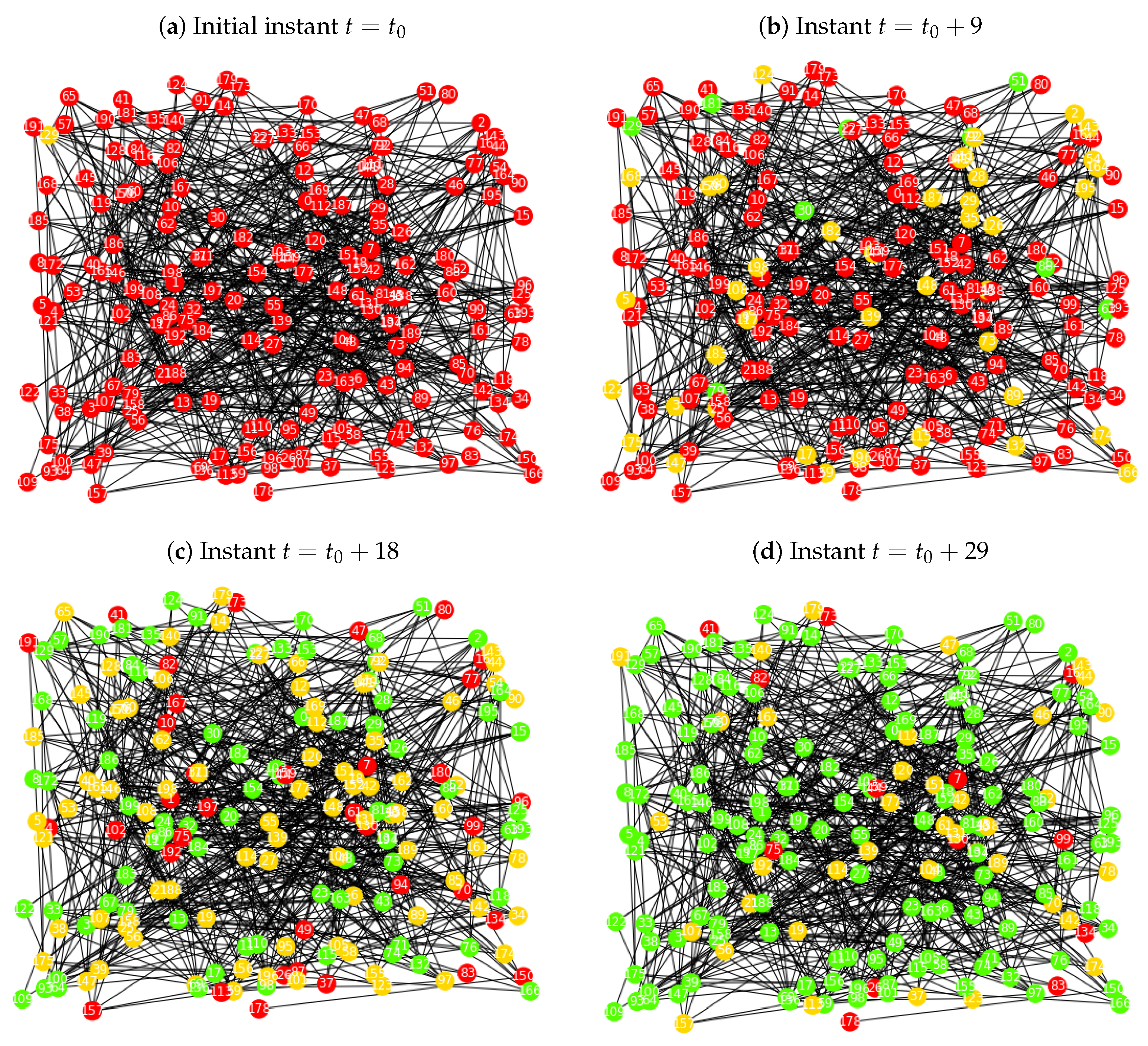
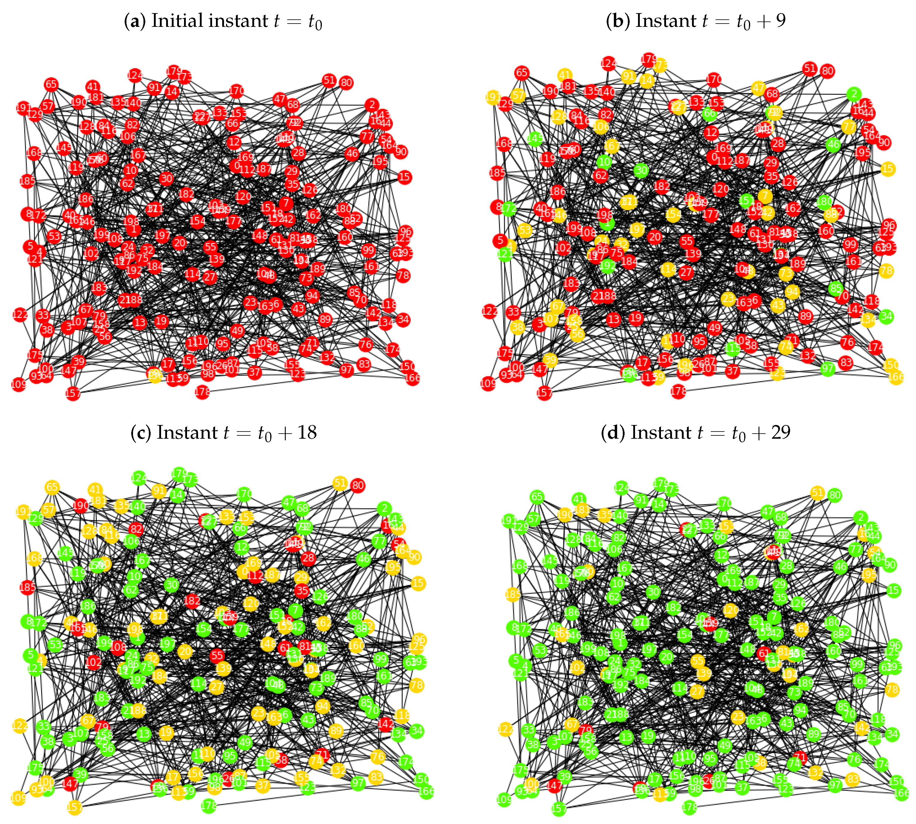
In Figure 2a is plotted the Erdös-Rényi network ${\mathcal{G}}_{(n,p)}$, at the initial instant $t=t_0$, where the node $x_{129}$ is the infected node or seed (yellow colour), which was chosen randomly, and has 9 neighbours, nodes $x_{13}$, $x_{35}$, $x_{65}$, $x_{79}$, $x_{91}$, $x_{92}$, $x_{103}$, $x_{170}$ and $x_{181}$. In the beginning of the process we have 1 infected node and 199 susceptibles (red colour). When we observe Figure 2b, which corresponds to iteration 9, at this point, there are individuals in all of the sets. Namely, 149 susceptibles, 42 infected and 9 recovered (green colour).

At instant $t=t_0+18$, Figure 2c, we observe that the proportion of nodes in the susceptible state is decreasing and that the proportion in the recovered state is increasing, as expected. At this instant there are 36 susceptible individuals, 86 infected and 78 recovered. In the last instant, the proportion of recovered nodes, is much greater than the other two, which means that the majority of the population is not able to get infected anymore and eventually the disease will disappear. In that way, we can see that 148 individuals belong in $R\left(t\right)$, 39 have the disease and 13 are still susceptible.

Note that, in the simulations presented in the different case studies, from the moment that the SIR epidemic process is initiated, there is a gradual change in the presence of the colours associated with the different states as time passes, starting with red, moving to yellow and ending with green. This graphical information translates into the initial predominance in the network of susceptible nodes, with a large number going on to become infected and then recovered.

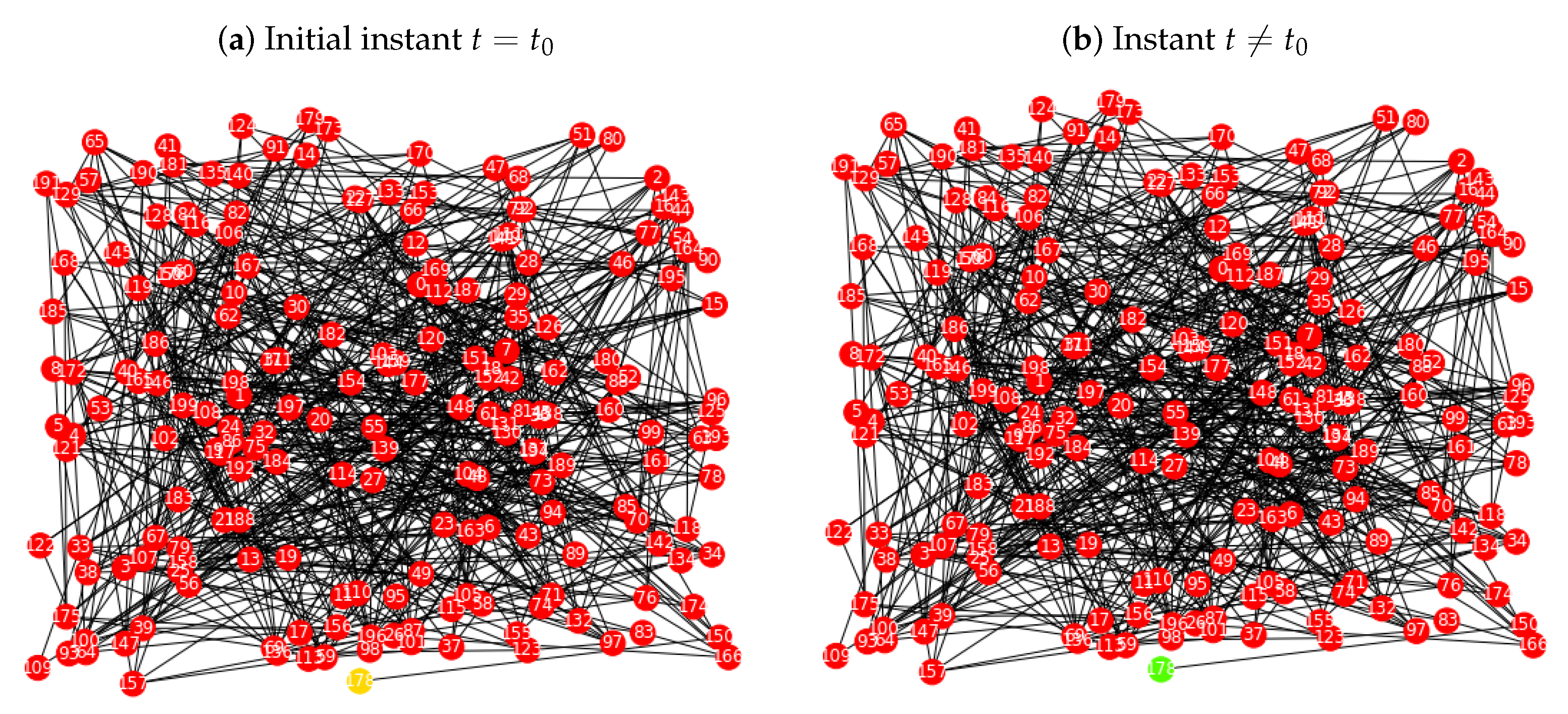
By contrast, in Figure 3a the same network is triggered by the node $x_{178}$, which was also randomly selected, and has only one neighbour, node $x_{150}$. In this case, there is no propagation of the disease and the process stops in step 2., see Figure 3b. In conclusion, in Figure 2 the propagation process exists, and in Figure 3 there is no epidemic occurring.

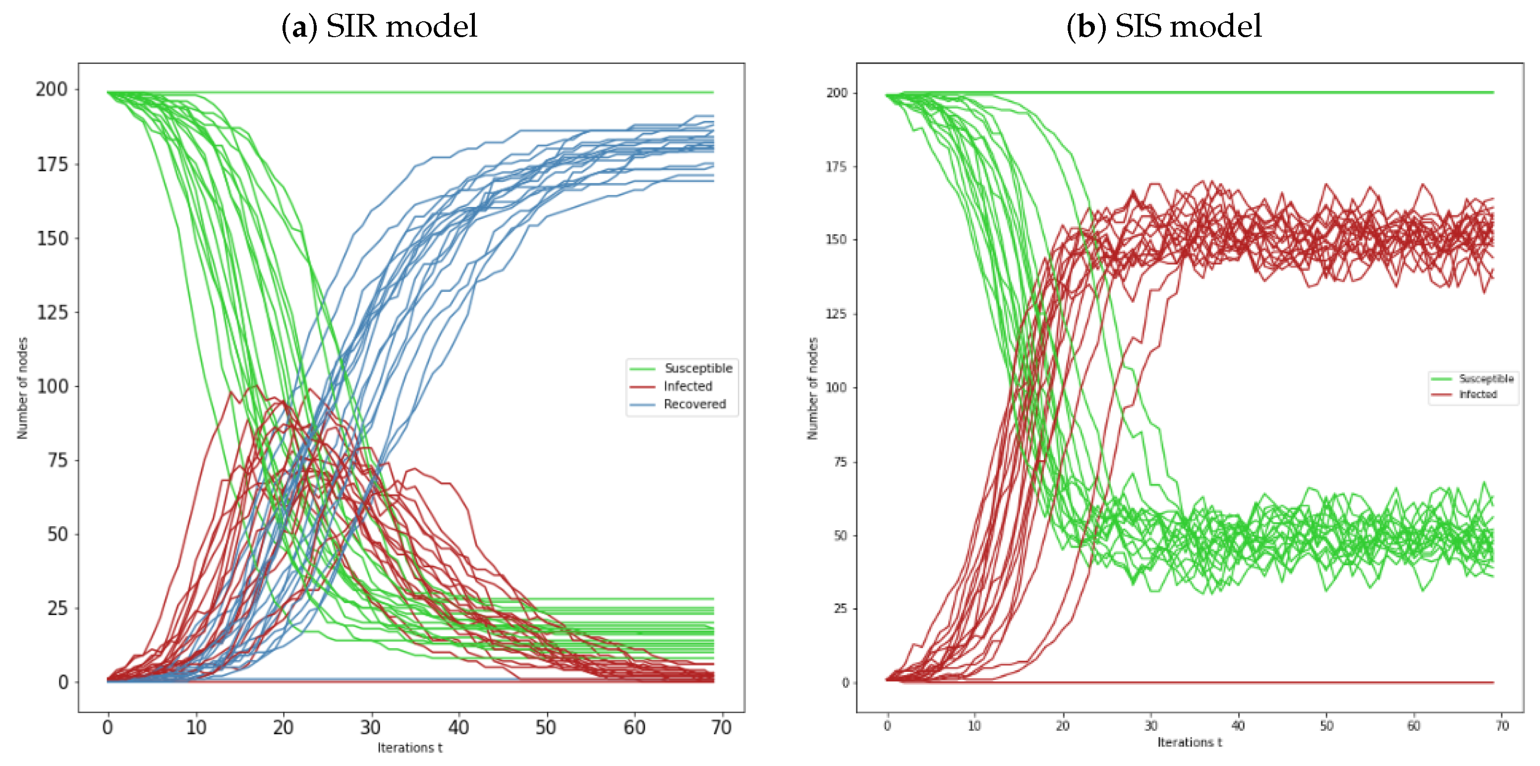
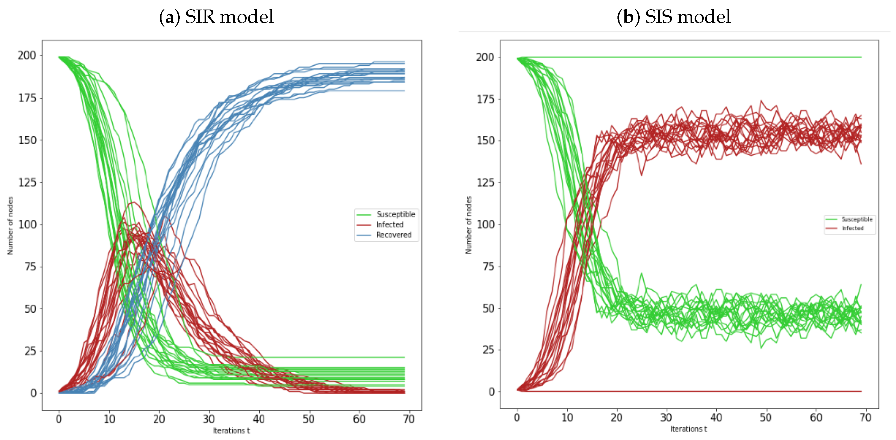
Now we consider the numerical simulations of 20 Erdös-Rényi networks, during 70 iterations, we maintained the same value for the networks order, $n=200$. For the SIR and SIS models represented by Figure 4a,b, we still have $p=0.028$ and $\tau =0.15$. Note that, we consider these values throughout all the subsections. In the first figure, we can see that most of the networks behave in a similar manner. The susceptible sets decrease (inverse sigmoid type) throughout time and the recovered size increases (sigmoid type). The infected sets increase and reach a peak, after that they start decreasing, reaching zero most of the time. Note that, there is at least one case where there is no epidemic spread, which graphically corresponds to the parallel lines.

In the SIS model, all the networks also behave similarly. In general, we see that both curves of this model decrease and increase in the same proportion, with behaviour of inverse sigmoid and sigmoid types, respectively. In both models, exist cases where there is no propagation. Note that, for the SIS model the curves of susceptible and infected individuals, after some iterations, have an oscillatory behaviour, which can be interpreted as peaks of infection.

6.2. Case Study 2: Seeds with Higher Degree Centrality

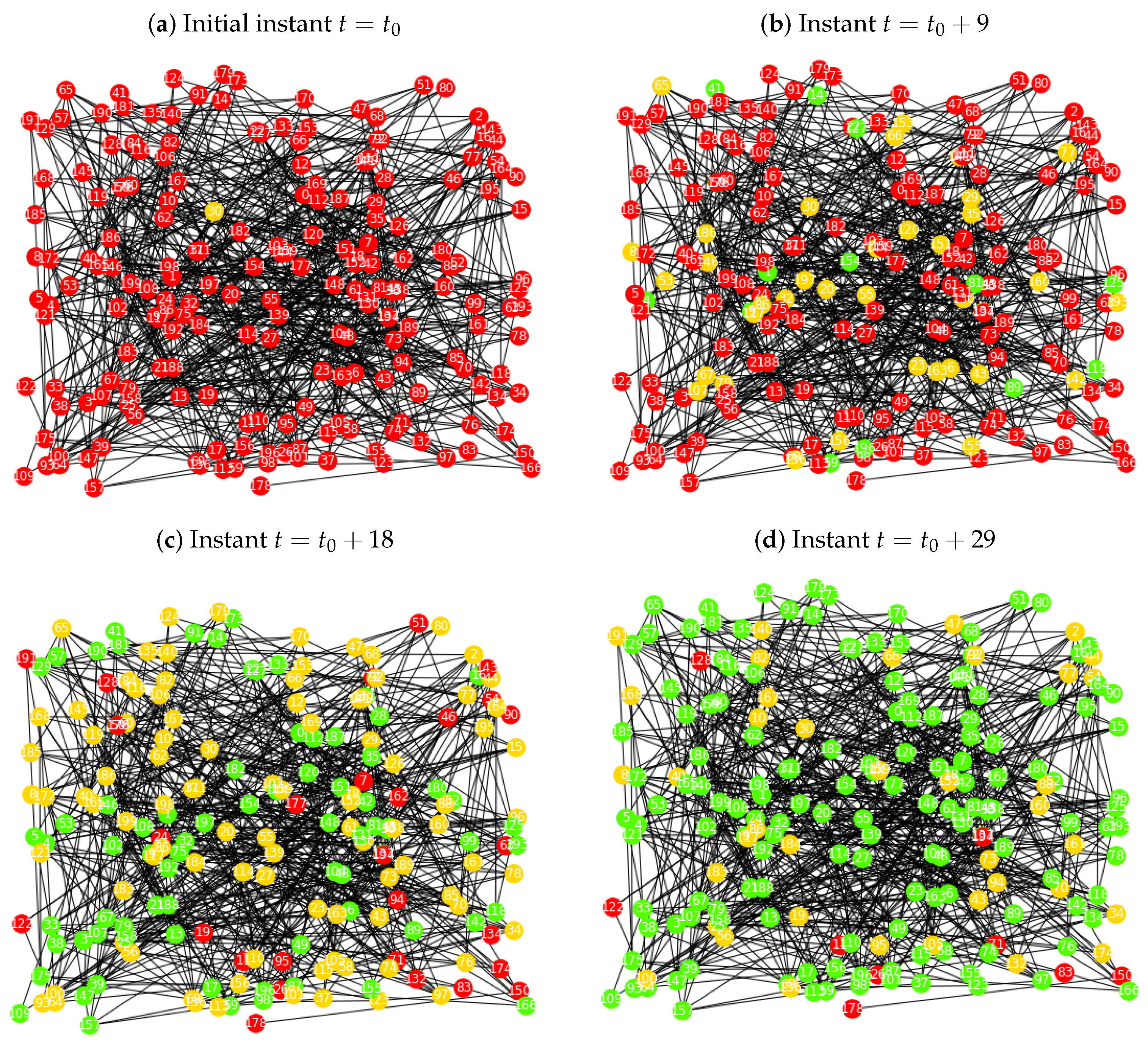
In order to compare the different choices for the only seed, throughout the case studies, we will preserve the network topology and the epidemic threshold $\tau =0.15$, established in case study 1. In Figure 5a is plotted the Erdös-Rényi network ${\mathcal{G}}_{(n,p)}$, at the initial instant $t=t_0$, where the node $x_{30}$ is the node with highest degree centrality, with 11 neighbours, nodes $x_8$, $x_9$, $x_{43}$, $x_{53}$, $x_{79}$, $x_{107}$, $x_{118}$, $x_{154}$, $x_{180}$, $x_{192}$ and $x_{196}$.

As we can observe in Figure 5b, after nine iterations there exists some infected individual and recovered, but very few in the last set. In the instant $t=t_0+18$, there are a large number of elements in the recovered group, and the proportion of infected elements is decreasing. In the last iteration, $t_{29}$, the majority of the population belongs to the recovered set, even though there are still a few elements in the infected and susceptible states. In this case study, the last iteration appears to have less elements in the susceptible set, when compared to the case study for a random seed.

Considering the degree centrality, we can observe in Figure 6a that a great amount of networks behave in the same manner, even though there exist cases where the propagation process happens faster. However, in this set of simulations for the SIR model, we have a case where strong epidemic spread only occurs after 20 iterations. In Figure 6b, most networks for the SIS model behave similarly. In both cases there are also examples where there is no epidemic.

6.3. Case Study 3: Seeds with Higher Closeness Centrality

In Figure 7a is plotted the Erdös-Rényi network ${\mathcal{G}}_{(n,p)}$, at the initial instant $t=t_0$, where the node $x_{136}$ is the node with highest closeness centrality value, with 11 neighbours. As we can observe in Figure 7b, in $t_9$, there are infected and recovered individuals (131 susceptible nodes, 50 infected and 19 recovered), but very few in the last set. At instant $t_{18}$, there are a large number of elements in the recovered group, and the number of infected elements is decreasing (28 susceptible nodes, 77 infected and 95 recovered). In the last iteration, $t_{29}$, the majority of the population belongs to the recovered set, even though there are still a few elements in the infected and susceptible state (9 susceptible nodes, 34 infected and 157 recovered). Note that, the last iteration of this simulation has similar outcomes as the last iteration of case study 2 presented in Figure 5d.

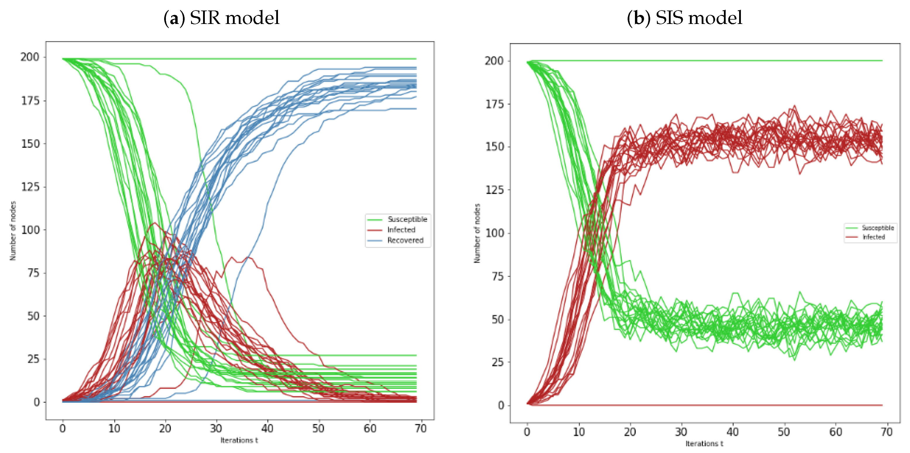
For this centrality measure, we can observe in Figure 8a a most of the networks for the SIR model have similar behaviour. However, we can again observe that there are some cases where strong epidemic spread occurs only after a higher number of iterations. The same can be seen in Figure 8b, for the SIS model. Only for the last model there were cases of no epidemic occurring. We observe that after the strong epidemic infection, there are several cases in which infection peaks occur. This phenomenon is justified by the presence of the oscillatory behaviour of the graphics.

In conclusion, we came across different choices of seeds, and in each example provided very similar simulations occurred. However, the network topology was preserved and perhaps this situation led to these results.

7. Discussion and Conclusions

In this paper we have considered the discrete form of SIR and SIS epidemic models, as general laws of epidemic spread in a population, with constant infection and recovery rates $\beta$ and $\gamma$, respectively, over Erdös-Rényi contact random networks ${\mathcal{G}}_{(n,p)}$. These propagation processes are also referred to as social contagion, as they are reminiscent of how a disease is transmitted among individuals. There are several approaches to define mathematical models for infectious diseases over networks. In our approach, we consider and formalize mathematically new probabilistic procedures for both SIR and SIS epidemic models, under very general conditions, regarding the topological structure of these random networks and the epidemic threshold, the rate of infection $\beta$ and recovery rate $\gamma$, associated with the studied models. However, we would highlight that an analogous formulation of these models in continuous-time can be found in [56].

With respect to the epidemic threshold $\tau$, defined by the spectral radius of the adjacency matrices associated with the contact networks ${\mathcal{G}}_{(n,p)}$, we obtained in Proposition 1 a characterization of $\tau$ depending on the network order n and for certain values of the probability p. The result is obtained by considering an asymptotic spectral approach and a sufficient condition on the connection probability p that restricts it to the phase regimes corresponding to the connected giant component. This result allowed us to establish some properties about the epidemic threshold dynamics in Proposition 2, reflecting an analysis on the global dynamics of the topological structure of the random networks under study. On the other hand, from the point of view of dynamical systems, we considered an explicit expression for the topological entropy of the Erdös-Rényi random networks, given by Definition 2. Consequently, a relationship between the epidemic threshold $\tau$ and the topological entropy $h_{top}\left({\mathcal{G}}_{(n,p)}\right)$ has been established. In addition, a relationship between the basic reproduction number $R_0$ and the topological entropy $h_{top}\left({\mathcal{G}}_{(n,p)}\right)$ was also stated. These relations are the main contributions of this work along with the establishment of the theoretical probabilistic procedures. Thus, the main result of this paper, Theorem 1, is proved. This connection reinforces the importance of dynamical systems theory in the epidemiology studies.

In Proposition 4 we presented conditions to trigger the infectious state $I\left(t\right)$, for the case when the seed node is a terminal node and for the general case. Furthermore, we concluded that the probability of initiating this state increases according to the degree of the seed node. At this point the maximum value for triggering the procedures is discussed, depending on the greater centrality degree of the networks. Thus, this result led us to use other centrality measures as a criterion of choice for the seed node, that have been presented in the numerical studies in Section 6. The paper is concluded with the discussion on the application specific centrality measures for the seed set and possible advantages of this choice over a random network. At the same time, the use of centrality measures in this context raises the analysis of local and global dynamics of the contact networks.

As a final observation, concerning the validation of the models, the computational implementation is evaluated according to the parameters considered, using the results established in Section 5. In other words, it is analyzed whether or not there is epidemic propagation for the parameters chosen. On the other hand, its implementation is strictly dependent on the local topology of the network, due to the epidemic propagation that is established in the theoretical procedures defined. This validation phase of the procedures is carried out in the computer implementation.