Stochastic Delay Differential Equations: A Comprehensive Approach for Understanding Biosystems with Application to Disease Modelling

Abstract

Mathematical models have been of great importance in various fields, especially for understanding the dynamical behaviour of biosystems. Several models, based on classical ordinary differential equations, delay differential equations, and stochastic processes are commonly employed to gain insights into these systems. However, there is potential to extend such models further by combining the features from the classical approaches. This work investigates stochastic delay differential equations (SDDEs)-based models to understand the behaviour of biosystems. Numerical techniques for solving these models that demonstrate a more robust representation of real-life scenarios are presented. Additionally, quantitative roles of delay and noise to gain a deeper understanding of their influence on the system’s overall behaviour are analysed. Subsequently, numerical simulations that illustrate the model’s robustness are provided and the results suggest that SDDEs provide a more comprehensive representation of many biological systems, effectively accounting for the uncertainties that arise in real-life situations.

1. Introduction

Over the years, many models have been formulated to closely represent the behaviour of biological systems using different forms of differential equations [1,2]. Until recently, many such models have ignored the potential impact of randomness within the system, which may be due to the complexity inherent in solving these models. Similarly, several models have not adequately included the effect of time delays in the system representations, and it is only recently that there has been a growing interest in understanding the implications of delays in dynamic systems. However, there is still relatively less work on models that combine both the influences of randomness and delay within the system, a gap that warrants attention [3]. Notably, the limited application of stochastic delay differential equations (SDDEs) is partly attributed to their inherent complexity in finding solutions, which can be particularly challenging when real-time simulation or rapid iterative modelling is required [4,5,6]. Moreover, SDDEs may demand significant computational resources and specialised numerical methods to ensure accuracy, rendering them less accessible to researchers with limited computational capabilities. These challenges underscore the imperative need for ongoing research aimed at developing more efficient numerical techniques and strategies to enhance the usability of SDDEs, particularly in large-scale and computationally demanding scenarios. Nevertheless, it is known that many real-life physical and biological systems are often exposed to the influences of several conditions that are not fully understood, making the explicit modelling of such a scenario less feasible. As such, there is an increasing need to extend the existing deterministic models into a more rigorous model that could incorporate the variations in the system dynamics. One of the ways of modelling such dynamics is an inclusion of the stochastic influence often referred to as the noise [7]. The natural extension of the deterministic model based on the ordinary differential equations (ODEs) could be an inclusion of delay or noise which leads to the system of stochastic or delay differential equation where the basic difference is that the SDEs account for the influence of randomness while DDEs account for the impact of pauses within the system [8]. Similarly, the standard extension of the DDEs-based model would therefore be a stochastic delay differential equation where these equations incorporated the effect of both noise and delay. However, the SDDEs are not just considered as the extension of the DDEs or SDEs, it is widely regarded as the generalisation of both the deterministic delay differential equations and the stochastic ordinary differential equations (SODEs) [9,10]. To date, it has been widely accepted that stochastic differential equations play a significant role in the modelling of several physical phenomena such as population dynamics, epidemiology, ecology, and many more. In the same way, the delay differential equation has been greatly used for the analysis and predictions in various areas of life sciences. The time delays included in the models often account for the dependency of the present state on the history [10]. Without loss of generality, both noise and delays are increasingly inevitable in biological systems and, due to their importance, an important part of the literature is now devoting attention towards the development and solutions. Some of the early references that discussed the SDDEs are the books by [11] which presented the small delay approximation of the equation and considered the effects of noise on the model equation. The basic introduction to the numerical analysis of these types of equations was presented by [3], where they considered Itô’s form of the SDDE and provided a numerical simulation of the solution using the Euler–Maruyama scheme. The survey of results involving the theory and stability of the differential equations involving perturbation and delays are documented in [12]. In their work, they discussed the survey of the existence and uniqueness of the solution of SDDEs together with the Markov properties, stochastic stability, and parameter estimations. Many more authors further extend the popular stochastic differential equation to incorporate delays and are used to describe technical devices such as control circuits, where the delay represents the time taken by a signal to travel to the control object together with the reaction time, while the noise accounts for the significant impact of randomness in the circuit performance that could influence the application with high precision. In finance, this equation could be used in developing an option pricing formula which will lead to the delayed Geometric Brownian Motion (GBM) and subsequently help obtain a modified Black–Scholes formula popularly used in economics for pricing European options. In summary, a delay is primarily introduced due to hidden processes that are not fully understood but are known to cause time lag [13,14], while the stochastic part is often included to account for the effect of randomness or behavioural representation which cannot be easily determined, and this could affect the overall dynamics of the system. In the subsequent section, we shall present the mathematical representation of this form of equation with their illustration in various physical modellings.

2. General Formulation

Since SDDEs emerge from both delay and stochastic differential equations, it is expected that some of the properties of stochastic and delay differential equations would apply to stochastic delay differential equations. Thus, we define an SDDE as a differential equation that includes at least one stochastic process term denoted by $W\left(t\right)$ and at least one time delay represented by $\tau$. Mathematically, let $0\le t_0<t_1,\cdots ,t_n<T<\infty$, and let $W\left(t\right)$ be a one-dimensional Wiener process defined on a filtered probability space $(\mathsf{\Omega },\mathcal{F},\mathbb{P})$, where $\mathsf{\Omega }$ represents the sample space, $\mathcal{F}$ denotes the filtration, and $\mathbb{P}$ is the probability. Then, a stochastic delay differential equation can be represented as follows:

$$\begin{array}{c}\hfill \left\{\begin{array}{cc}dy\left(t\right)\hfill & =f\left(t,y\left(t\right),y(t-\tau )\right)dt+g\left(t,y\left(t\right),y(t-\tau )\right)dW\left(t\right),t\in [0,T],\hfill \\ \\ y\left(t\right)\hfill & =\mathsf{\Phi }\left(t\right),t\in [-\tau ,0],y\in \mathbb{R},\mathsf{\Phi }\left(t\right)\in \mathbb{R}.\hfill \end{array}\right.\end{array}$$

(1)

$W\left(t\right)$ represent the Wiener process with zero mean and variance ${\sigma }^2$, while the drift coefficient $f:[0,T]\times {\mathbb{R}}^d\times {\mathbb{R}}^d⟶{\mathbb{R}}^d$ and the diffusion coefficient $g:[0,T]\times {\mathbb{R}}^d\times {\mathbb{R}}^d⟶{\mathbb{R}}^d$ are d-dimensional and assumed to be Lipschitz continuous.

Furthermore, the equation given in (1) can be expressed in an integral form as

$$\begin{array}{c}\hfill \left\{\begin{array}{cc}y\left(t\right)-y\left(0\right)\hfill & ={\int }_0^{t}f\left(s,y\left(s\right),y(s-\tau )\right)ds+g\left(s,y\left(s\right),y(s-\tau )\right)dW\left(s\right),t\in [0,T]\hfill \\ \\ y\left(t\right)\hfill & =\mathsf{\Phi }\left(t\right),t\in [-\tau ,0],y\in \mathbb{R},\mathsf{\Phi }\left(t\right)\in \mathbb{R}.\hfill \end{array}\right.\end{array}$$

(2)

The second integral in (2) is often referred to as the stochastic integral in the Itô sense [15].

2.1. Numerical Scheme for SDDEs

In this section, we outline the numerical approach for solving Equation (2). To begin, we establish a set of equidistant mesh points within the interval $[0,T]$, denoted as $h=\frac{T}{N}$ and $t_n=nh$, where n ranges from 0 to N. Additionally, we assume that, for a given step size h, there exists an integer value, denoted as m, such that the time delay can be expressed as $\tau =mh$. For all instances where the indices satisfy $n-m\le 0$, we set ${\tilde{y}}_{n-m}$ equal to $\mathsf{\Phi }(t_n-\tau )$. In all other cases, the numerical approximation of (1) takes the following form:

$${\tilde{y}}_{n+1}={\tilde{y}}_n+\varphi (h,{\tilde{y}}_n,{\tilde{y}}_{n-m},I_{\varphi }),n=0,\cdots ,N-1.$$

(3)

We note that the increment function $\varphi (h,{\tilde{y}}_n,{\tilde{y}}_{n-m},I_{\varphi })$ represents the computation which updates the numerical approximation of the solution at the next time step based on the information available at the current time step n and the delayed information from time step $n-m$. Similarly, the increment function $\varphi (h,{\tilde{y}}_n,{\tilde{y}}_{n-m},I_{\varphi })$: $\mathbb{R}\times \mathbb{R}⟶\mathbb{R}$ includes a finite number of multiple Itô-integrals [9,16,17] of the form:

$$I_{(j_1,\cdots ,j_l),h}={\int }_t^{t+h}{\int }_t^{s_l}\cdots {\int }_t^{s_2}d{W}^{j_1}\left(s_1\right)\cdots d{W}^{j_{l-1}}\left(s_{l-1}\right)d{W}^{j_l}\left(s_l\right),$$

(4)

where $j_i\in \{0,1\}$ and $d{W}^0\left(t\right)=dt$ , and with $t=t_n$ for (3), we denote $I_{\varphi }$ the collection of Itô-integrals required to compute the increment function $\varphi$.

2.1.1. Euler–Maruyama Scheme

The Euler–Maruyama scheme is a popular method for numerically solving Stochastic Differential Equations (SDEs). It is also widely used for solving Stochastic Delay Differential Equations (SDDEs). The basic idea behind the method is to discretise the time domain into small intervals and approximate the solution at the end of each interval by adding the deterministic and stochastic terms. The method is derived from the Taylor expansion of the solution, and it is a first-order weak scheme that converges in the mean-square sense. Suppose we consider the SDDE given in (1), where $Y\left(t\right)$ is the state variable at time t, $f(t,Y(t),Y(t-\tau \left)\right)$ is the drift term, $g(t,Y(t),Y(t-\tau \left)\right)$ is the diffusion term, $W\left(t\right)$ is the Wiener process, and $\tau$ is the delay time. The delay term makes the numerical solution more challenging since it involves the state variable at a previous time. To apply the Euler–Maruyama scheme to SDDEs, we first discretise the time domain into N equal intervals of length $\mathsf{\Delta }t=(T-t_0)/N$, where T is the final time and $t_0$ is the initial time. Then, we can approximate the solution at the end of each interval using the following formula:

$$Y\left(t_{n+1}\right)=Y\left(t_n\right)+f(t_n,Y\left(t_n\right),Y(t_n-\tau ))\mathsf{\Delta }t+g(t_n,Y\left(t_n\right),Y(t_n-\tau ))\mathsf{\Delta }W\left(t_n\right).$$

(5)

$Y\left(t_n\right)$ is the numerical solution at time $t_n$, and $\mathsf{\Delta }W\left(t_n\right)$ is the Wiener increment over the time interval $[t_n,t_n+1]$. The Wiener increments are normally distributed with mean 0 and variance $\mathsf{\Delta }t$, which implies that $\mathsf{\Delta }W\left(t_n\right)\sim N(0,\mathsf{\Delta }t)$. To obtain the numerical solution, we start from the initial condition $Y\left(t_0\right)=Y_0$ and compute $Y(t_n+1)$ recursively using the above formula. We generate the Wiener increments using a random number generator, and we use interpolation or extrapolation techniques to evaluate the delay term $f(t_n,Y\left(t_n\right),Y(t_n-\tau ))$ and $f(t_n,Y\left(t_n\right),Y(t_n-\tau ))$. The Euler–Maruyama scheme is a simple and efficient method for solving SDDEs, but it is only a first-order weak scheme that may not be accurate for complex SDDEs. However, it can be extended to higher-order schemes such as the Milstein method to improve the accuracy.

2.1.2. Milstein Scheme

The Milstein scheme is a popular numerical method for approximating the solutions of stochastic delay differential equations. It is an extension of the Euler–Maruyama method, which is a simple but often inaccurate method for approximating solutions of stochastic differential equations [18]. The Milstein scheme improves on the Euler–Maruyama method by including a correction term that takes into account the second-order moments of the Wiener process.

Consider the one-dimensional stochastic delay differential equation given in (1). The Milstein approximation for the solution $Y\left(t\right)$ at a time step $t_n$ with time increment $\mathsf{\Delta }t$ is given by

$$\begin{array}{cc}\hfill Y\left(t_{n+1}\right)& =Y\left(t_n\right)+f(t_n,Y\left(t_n\right),Y(t_n-\tau ))\mathsf{\Delta }t+g(t_n,Y\left(t_n\right),Y(t_n-\tau ))\mathsf{\Delta }W\left(t_n\right)\hfill \\ \hfill & +\frac{1}{2}g(t_n,Y\left(t_n\right),Y(t_n-\tau ))g^{\prime }(t_n,Y\left(t_n\right),Y(t_n-\tau ))[{\left(\mathsf{\Delta }W\left(t_n\right)\right)}^2-\mathsf{\Delta }t],\hfill \end{array}$$

(6)

where $\mathsf{\Delta }{W}_n=W_{t_{n+1}}-W_{t_n}$ is the increment of the Wiener process over the time step $\mathsf{\Delta }t$. The first term on the right-hand side of (6) represents the deterministic drift term, which accounts for the delayed influence of the process. The second term is the random term, which accounts for the stochastic fluctuations in the process. The third term is the correction term, which accounts for the second-order moments of the Wiener process. The fourth term is a further correction term that accounts for the covariance between the Wiener process at different time steps. We present the algorithm used for Milstein scheme in Listing 1.

Listing 1. Implementation algorithm.

1. Define the initial condition Y[0] and the time interval [0,T]. 2. Define the time step and the number of time steps N = (T-t_0)/dt 3. Initialize the solution array Y with Y[0] and the Wiener process array W with increments W(t_n). 4. For n = 1 to N do the following: a. Compute the drift term f(t_n,Y(t_n),Y(t_n−tau)) and the diffusion term g(t_n,Y(t_n),Y(t_n−tau)). b. Generate a Wiener increment W(t_n) using a random no generator. c. Compute the approximation Y(t_{n+1}) using the Euler-Maruyama or Milstein formula . d. Append Y(t_{n+1}) to the solution array Y and W(t_n) to the    Wiener process array W. 5. Return the solution array Y and the Wiener process array W.

The above pseudo-code implements the numerical scheme for a one-dimensional stochastic delay differential equation with the delayed term and the noise term. The solution array Y is initialised with the initial value $Y_0$, and then the scheme is applied iteratively to compute the solution values at each time step. For the Milstein scheme, it includes four terms: the deterministic drift term, the random term, the correction term, and the covariance correction term. Each term is computed using the current solution value and the Wiener process increment at the current time step. The scheme has a strong convergence rate of order 1.5 for linear equations and order 1 for non-linear equations [19].

3. The Evolution of Modelling to SDDEs

Here, we outline the evolution of mathematical modelling, progressing from ordinary differential equations to the system of stochastic delay differential equations. We emphasise the expansion of each model to account for the complexity of overall system behaviour. To begin, we investigate population dynamics. Subsequently, we delve into the applications of SDDEs in various modelling domains, including epidemiology and ecology. Finally, we present the development of the model equations and discuss the rationale behind modifying existing models.

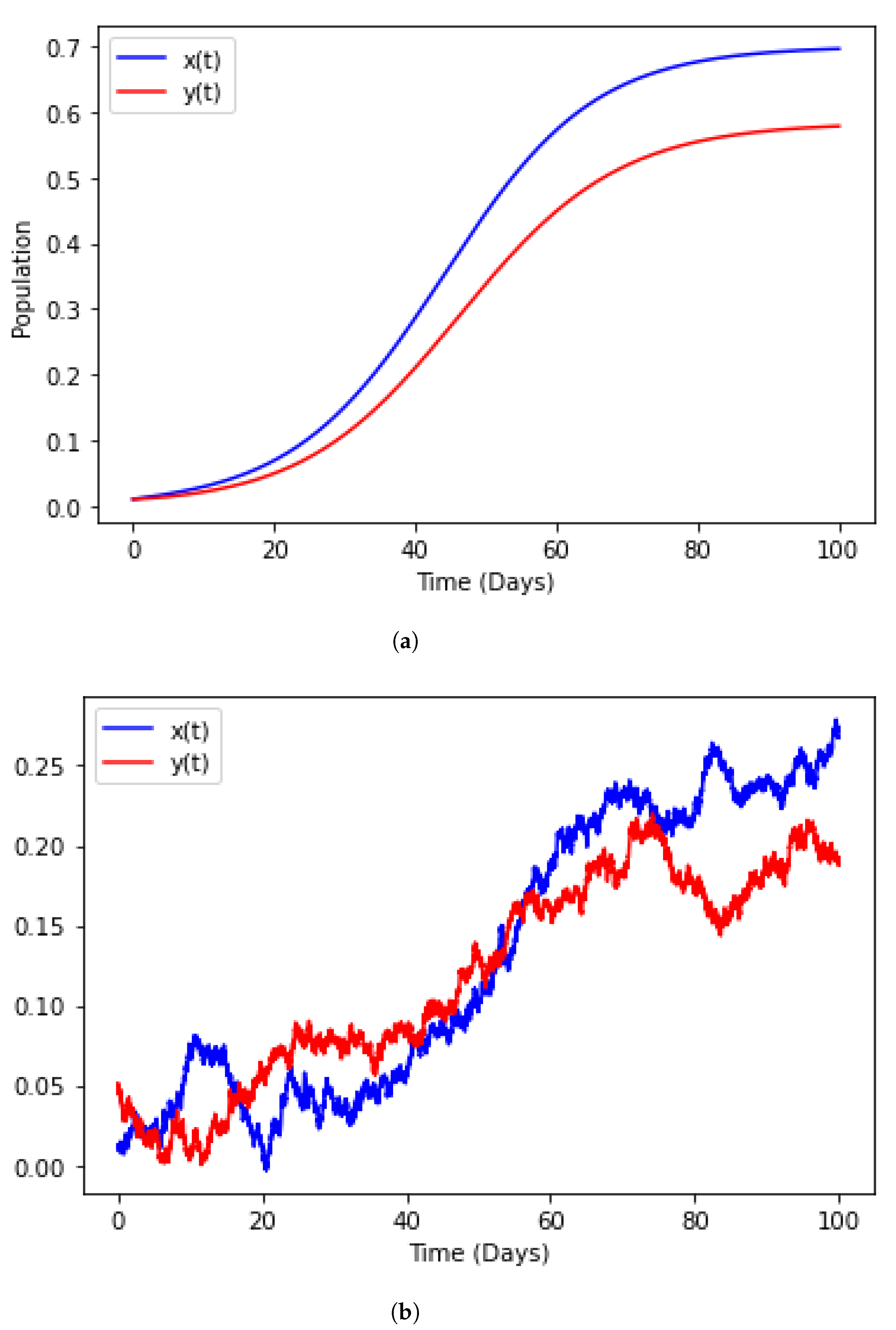
3.1. Population Dynamics

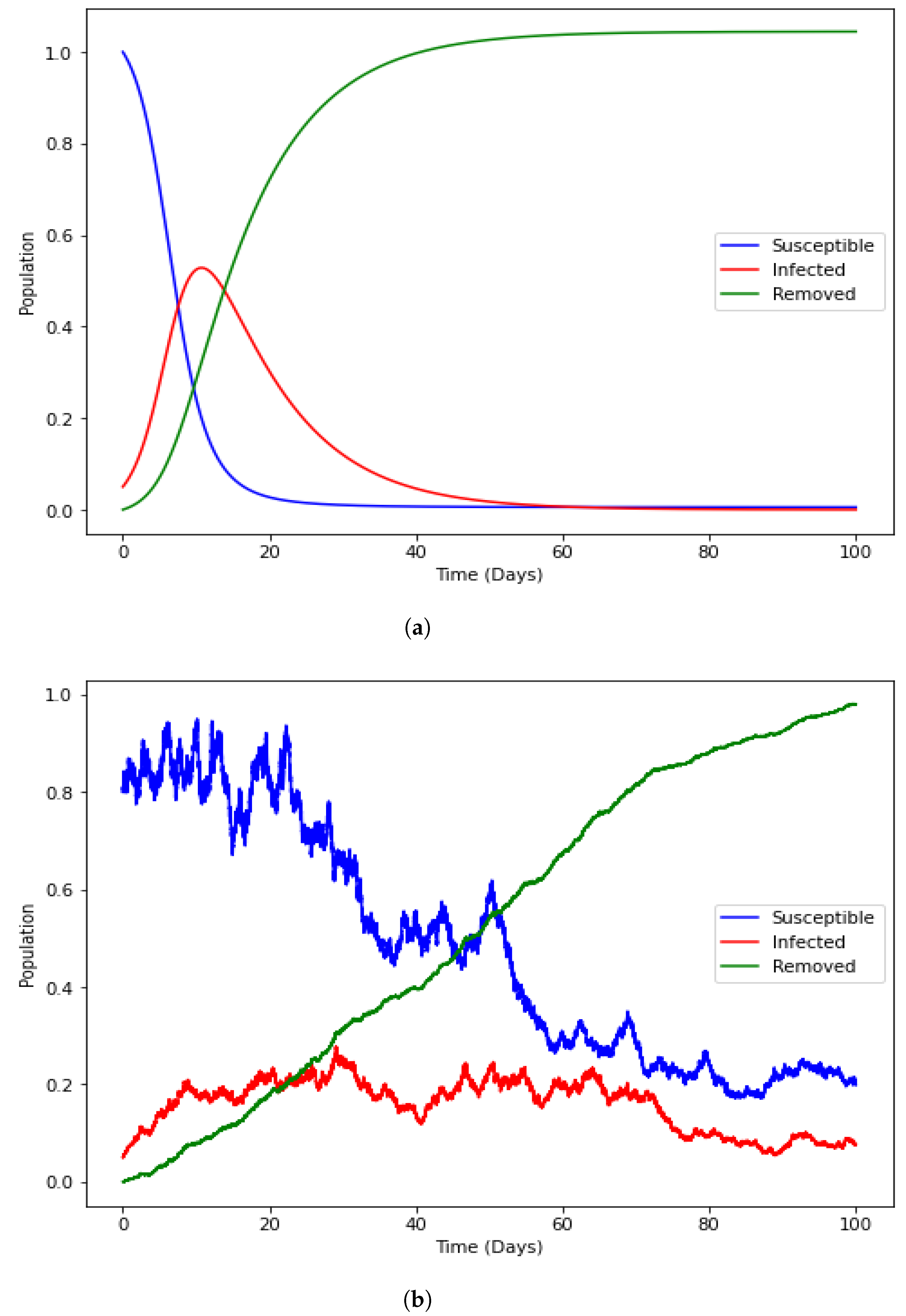
It is well-established that population dynamics discusses the changes in the size and composition of populations over time. The study of population dynamics has a long and fascinating history, from early mathematical models of exponential growth to more recent models that incorporate delays and stochasticity. Here, we will explore the evolution of population dynamics models from exponential growth to stochastic delay differential equations. The simplest model of population growth is the exponential growth model. This model assumes that the rate of population growth is proportional to the size of the population. Mathematically, this can be represented as:

$$\frac{dP}{dt}=rP,$$

(7)

where P is the population size, t is time, and r is the intrinsic growth rate. This model predicts that populations will grow without bounds unless there are limiting factors, such as resource availability [20]. As a result of the limitation of this equation, Verhulst proposed the logistic equation, which is a modification of the exponential growth model that takes into account limiting factors. The logistic equation assumes that as the population size approaches a carrying capacity, the rate of growth slows down. Mathematically, this can be represented as

$$\frac{dP}{dt}=rP\left(1-\frac{P}{K}\right).$$

(8)

The parameter K represents the carrying capacity and the logistic equation predicts that populations will stabilise at a carrying capacity. The equation has been widely used to model growth in different phenomena and was accepted to better explain population dynamics. Even though this model is widely used, it is worth noting that the logistic equation assumes that the effects of limiting factors on population growth are instantaneous. However, in reality, there are often delays between changes in limiting factors and changes in population growth rates. This led to the further modification by Hutchinson [21] to have a delay logistic equation that takes into account these delays. Mathematically, this is represented as

$$\frac{dP}{dt}=rP\left(1-\frac{P(t-\tau )}{K}\right).$$

The difference is the inclusion of the delay parameter $\tau$, which thereby allows for the equation to predict that populations will exhibit oscillatory behaviour before stabilising at a carrying capacity. We note that the delay logistic equation can be transformed to become $\frac{dy}{dt}=ry\left(1-y(t-\tau )\right)$. By considering the equation, we could observe that the equation assumes that the effects of limiting factors on population growth are deterministic. In reality, there are often random fluctuations in the environment that affect population growth rates. Hence, the impact of noise could also be introduced into the system such that we will have $r\left(t\right)=r\left(t\right)+\eta \left(t\right)$, where $\eta \left(t\right)$ is the Gaussian white noise with a time-varying intensity ${\sigma }^2\left(t\right)$ [22]. Thus, we could write $\eta \left(t\right)dt=\sigma \left(t\right)d{W}_t$, with $W_t$ representing the Wiener process. Therefore, the stochastic version of the delay logistic equation could be written as

$$dy\left(t\right)=ry\left(1-y(t-\tau )\right)dt+\sigma y\left(1-y(t-\tau )\right)d{W}_t,$$

(9)

which can therefore predict that populations will exhibit both deterministic and stochastic behaviour. In Figure 1, we present the effect of delay and noise in population dynamics using logistic equation.

3.2. Epidemiology

In infectious disease modelling, the population is often classified into different compartments based on the population status. The epidemic SIR (Susceptible-Infectious-Recovered) model has been widely used to study the spread of infectious diseases in populations. The classical model assumes that the population is well-mixed and that the transmission rate is constant over time. However, in real-world scenarios, there are often time lags between the exposure of individuals to the disease and their infectiousness. The classical SIR model is based on ordinary differential equations (ODEs) and assumes that the transition between compartments occurs instantaneously. However, this assumption is not always realistic, especially for diseases with a long incubation period or with a significant delay in the onset of infectiousness. As a result, the SIR model has been extended to delay differential equations (DDEs) which are used to model such delays in the transmission process [9]. Similarly, SDEs are used to capture the randomness in the transmission process but much work does not consider the scenario wherein there are both delay and randomness in the transmission process. Hence, we shall present the stochastic delayed model for the widely used epidemic SIR model. Mathematically, the classical SIR model is a set of three coupled ODEs that describe the evolution of the three compartments of a population: susceptible (S), infectious (I), and recovered (R). The equations are given by

$$\begin{array}{cc}\hfill \frac{dS}{dt}& =-\beta SI,\hfill \\ \hfill \frac{dI}{dt}& =\beta SI-\gamma I,\hfill \\ \hfill \frac{dR}{dt}& =\gamma I,\hfill \end{array}$$

(10)

where $\beta$ is the transmission rate and $\gamma$ is the recovery rate. The total population size $N=S+I+R$ is assumed to be constant. The delayed version of this model indicates that there may be a time delay between infection and infectiousness. The simple form of the delay inclusion could be given as

$$\begin{array}{cc}\hfill \frac{dS}{dt}& =-\beta S\left(t\right)I(t-\tau ),\hfill \\ \hfill \frac{dI}{dt}& =\beta S\left(t\right)I(t-\tau )-\gamma I\left(t\right),\hfill \\ \hfill \frac{dR}{dt}& =\gamma I(t-\tau ),\hfill \end{array}$$

(11)

where $\tau$ is the time delay between infection and infectiousness. The delay SIR model has been used to model the spread of diseases such as tuberculosis [23], COVID-19 [10,24,25,26] and HIV [27,28], which have a long incubation period. We note that the delay SIR model assumes that the time delay is constant and deterministic. However, in many cases, the time delay may be random and unpredictable. Therefore, to incorporate the randomness in the delay, there is a need for the representation of the system using the stochastic delay SIR model. Hence, the model could take the following form:

$$\begin{array}{cc}\hfill dS\left(t\right)& =-\beta S\left(t\right)I(t-\tau )dt+{\sigma }_{S}d{W}_t,\hfill \\ \hfill dI\left(t\right)& =\beta S\left(t\right)I(t-\tau )-\gamma I\left(t\right)+{\sigma }_{I}d{W}_t,\hfill \\ \hfill dR\left(t\right)& =\gamma I(t-\tau )dt.\hfill \end{array}$$

(12)

where $W_t$ represent independent Wiener processes and $\sigma$ is the strength of the noise, which are motivated by the randomness and uncertainties inherent in the spread of the disease. We present the illustration of the effect of delay and noise in population dynamics using SIR model in Figure 2.

3.3. Ross–Macdonald Malaria Model

The Ross–Macdonald model is a well-known mathematical model used to study the transmission dynamics of malaria. The model started with Ross in 1911 and was designed to describe the transmission of malaria. The concepts were a source of inspiration for a group of medical entomologists, and beginning in 1950, there was a significant advancement in the field. This was largely due to the combination of the theoretical work of George Macdonald and the empirical work of his colleagues [29]. Their work provided a complete understanding of transmission dynamics and control, and successfully linked the models and the metrics. To date, this model serves as the basis of countless models for vector-borne diseases. However, we consider the Aron and May version of the Ross–Macdonald model [30]. This famous model used the ordinary differential equation, which is given as

$$\begin{array}{cc}\hfill \frac{dx}{dt}& =maby(1-x)-rx,\hfill \\ \hfill \frac{dy}{dt}& =acx(1-y)-\mu y.\hfill \end{array}$$

(13)

where $x\left(t\right)$ and $y\left(t\right)$ are the proportion of infected humans and mosquitoes at time t is the prevalence of malaria, m is the number of mosquitoes per human host, the pathogen’s host is denoted by a, the proportion of bites by infectious mosquitoes that infect a human is represented by b. Altogether, the product $mabz$ is the force of infection or “happenings” rate for human infections and the instantaneous death rate is denoted by $\nu$. Further explanation of each parameter can be found in [29,31]. By considering this model, it could be observed that the influence of the time-varying nature of the vector and host populations was not considered. To account for this, there is therefore a need to incorporate a time delay. According to [31], the feedback dynamics from mosquito to human and back to mosquito involve considerable time delays due to the incubation periods of the parasites. Therefore, a delayed model is required to explicitly account for the incubation periods of parasites within the human and the mosquito. Thus, this leads to an extension of the model to a delayed Ross–Macdonald model which is given as [31]

$$\begin{array}{cc}\hfill \frac{dx}{dt}& =maby(t-{\tau }_1)\left(1-x(t-{\tau }_1)\right)e^{-r{\tau }_1}-rx,\hfill \\ \hfill \frac{dy}{dt}& =acx(t-{\tau }_2)\left(1-y(t-{\tau }_2)\right)e^{-r{\tau }_2}-\mu y,\hfill \end{array}$$

(14)

where ${\tau }_1,{\tau }_2$ represents the delays. These delays represent the time it takes for an infected mosquito to transmit the disease to a human, and the time it takes for an infected human to become infectious. Ruan et al. [31] used this model to calculate the basic reproduction number $R_0$ and carry out the sensitivity analysis of the $R_0$ on the incubation periods. As the model adequately accounts for the effect of time delays on the basic reproduction number, it does not include the influence of additional disturbance and randomness. Hence, there is need for a further modification that would include the impact of delays and fluctuations. The delay would capture the fact that infected individuals do not become infectious immediately after being bitten by a mosquito, but instead take a certain amount of time to develop symptoms and become infectious themselves. Similarly, recovered individuals do not immediately lose their immunity to the disease, but instead, retain it for a certain amount of time, while the addition of a stochastic part will account for the random fluctuations in the transmission and recovery rates. This will therefore lead to a stochastic delay differential equation (SDDE) model of the form

$$\begin{array}{cc}\hfill \frac{dx}{dt}& =maby(t-{\tau }_1)\left(1-x(t-{\tau }_1)\right)e^{-r{\tau }_1}-rx+{\sigma }_{x}d{W}_t,\hfill \\ \hfill \frac{dy}{dt}& =acx(t-{\tau }_2)\left(1-y(t-{\tau }_2)\right)e^{-r{\tau }_2}-\mu y+{\sigma }_{y}d{W}_t,\hfill \end{array}$$

(15)

where $W_t$ are independent Wiener processes representing the random fluctuations within the population and ${\sigma }_i$ denoting the corresponding deviations. The illustration of the effect of delay and noise using the malaria model (15) is presented in Figure 3.

4. Numerical Illustration

In this section, we present the numerical simulation of the SIR model with vaccination and quarantine which is presented in [32]. The model considered a population of five compartments which are grouped into Susceptible $S\left(t\right)$, Vaccinated class $V\left(t\right)$, Infected class $I\left(t\right)$, Quarantine class $Q\left(t\right)$, and recovered class $R\left(t\right)$. Total population is expressed as $N\left(t\right)=S\left(t\right)+V\left(t\right)+I\left(t\right)+Q\left(t\right)+R\left(t\right)$. Assuming the population is constant, the birth rate is denoted by $\mu$, while $\beta$ represents the transmission rate (the rate at which susceptible individuals become infected). $\gamma$ is the transmission rate and the rate at which susceptible individuals become vaccinated is represented by ${\omega }_1$. Similarly, the quarantine rate is denoted by ${\theta }_1$, while the rate at which quarantined individuals recovered is represented by ${\alpha }_2$, while ${\alpha }_1$ is the rate at which infected individuals recover and become immune. Hence, the model is presented as

$$\begin{array}{cc}\hfill \frac{dS}{dt}& =\mu -\beta SI-(\gamma +{\omega }_1)S,\hfill \\ \hfill \frac{dV}{dt}& ={\omega }_{1}S-\gamma V,\hfill \\ \hfill \frac{dI}{dt}& =\beta SI-(\gamma +{\theta }_1+{\alpha }_1)I,\hfill \\ \hfill \frac{dQ}{dt}& ={\theta }_{1}I-(\gamma +{\alpha }_2)Q,\hfill \\ \hfill \frac{dR}{dt}& ={\alpha }_{1}I-\gamma R+{\alpha }_{2}Q.\hfill \end{array}$$

(16)

The description of parameters in the model (16) is presented in

Table 1. Description of the model parameters.

Parameter	Description
$S\left(t\right)$	Susceptible population at time t. This is the group of individuals who are not infected but are at risk of becoming infected.
$V\left(t\right)$	Vaccinated population at time t which represents individuals who have been vaccinated against the disease.
$I\left(t\right)$	Infectious population at time t. The group of individuals currently infected and capable of spreading the disease.
$Q\left(t\right)$	Quarantined population at time t. Individuals who are quarantined due to infection.
$R\left(t\right)$	Recovered population at time t. Includes individuals who have recovered from the disease and are no longer infectious.
$\mu$	Recruitment rate of the susceptible population, i.e., the rate at which individuals enter the susceptible group.
$\beta$	Transmission rate of the disease which is the rate at which susceptible individuals become infected when they come into contact with infectious individuals.
$\tau$	Time delay indicating that newly infected individuals do not become infectious immediately but after a delay of $\tau$ time units.
$\gamma$	Recovery rate, i.e., the rate at which infected individuals recover and move to the recovered compartment.
${\omega }_1$	Rate at which susceptible individuals become vaccinated.
${\theta }_1$	Rate at which infected individuals are placed in quarantine.
${\alpha }_1$	Rate at which the quarantined individuals are recovered.
${\alpha }_2$	Rate at which individuals in quarantine transition to the recovered compartment.
${\sigma }_S,{\sigma }_V,{\sigma }_I,{\sigma }_Q,{\sigma }_R$	Represent the level of fluctuation within each model compartment.

.

Firstly, we shall present the quantitative analysis of this model after which we will incorporate the delay parameter and randomness in the model. We will discuss the positivity condition and then examine the equilibria as well as the reproduction number.

4.1. Positivity of the Solution

Here, we show that the model (16) satisfies the positivity condition provided that $N\left(t\right)=S\left(t\right)+V\left(t\right)+I\left(t\right)+Q\left(t\right)+R\left(t\right)$. Then, by considering each compartment of (16), we have that

$$\frac{dN}{dt}=\frac{dS}{dt}+\frac{dV}{dt}+\frac{dI}{dt}+\frac{dQ}{dt}+\frac{dR}{dt}.$$

So,

$$\begin{array}{cc}\hfill \frac{d}{dt}(S+V+I+Q+R)& =\mu -\gamma (S+V+I+Q+R),\hfill \\ \hfill \frac{dN}{dt}& =\mu -\gamma N,\hfill \\ \hfill N{e}^{\gamma t}& =\int \mu e^{\gamma t},\hfill \\ \hfill N\left(t\right)& =\frac{\mu }{\gamma }+c{e}^{-\gamma t}.\hfill \end{array}$$

At $t=0$, $N\left(0\right)=N_0=\frac{\mu }{\gamma }+c$.

Hence, $N\left(t\right)$ at any time t is given by,

$$N\left(t\right)=\frac{\mu }{\gamma }+\left(N_0-\frac{\mu }{\gamma }\right)e^{-\gamma t},$$

(17)

where

$$\underset{t⟶\infty }{lim}N\left(t\right)=\frac{\mu }{\gamma }>0.$$

4.2. Equilibrium

We shall determine both the disease-free equilibrium and the endemic equilibrium. To find the disease-free equilibrium, we take $I=Q=R=0$, which means that there are no infected, quarantined, or recovered individuals in the population. By substituting into the equations, we have

$$\begin{array}{cc}\hfill \frac{dS}{dt}& =\mu -\beta SI-(\gamma +{\omega }_1)S=0.\hfill \\ \hfill \frac{dV}{dt}& ={\omega }_{1}S-\gamma V=0.\hfill \end{array}$$

From the second equation, we obtain $V=\frac{{\omega }_1}{\gamma }S$. Therefore,

$$\begin{array}{cc}\hfill S^{*}& =\frac{\mu }{\gamma +{\omega }_1}.\hfill \end{array}$$

Now, substituting this expression for S into the equation for V, we obtain

$$\begin{array}{cc}\hfill V^{*}& =\frac{{\omega }_1}{\gamma }{S}^{*},\hfill \\ \hfill & =\frac{{\omega }_1}{\gamma }\frac{\mu }{\gamma +{\omega }_1},\hfill \\ \hfill & =\frac{\mu {\omega }_1}{{\gamma }^2+{\omega }_1\gamma }.\hfill \end{array}$$

Thus, the disease-free equilibrium of the system is

$$(S_0,V_0,I_0,Q_0,R_0)=\left(\frac{\mu }{\gamma +{\omega }_1},\frac{\mu {\omega }_1}{{\gamma }^2+{\omega }_1\gamma },0,0,0\right).$$

Similarly, for the endemic equilibrium, we need to solve the system of equations obtained by setting the derivatives to zero:

$$\begin{array}{cc}\hfill \frac{dS}{dt}& =0=\mu -\beta SI-(\gamma +{\omega }_1)S,\hfill \\ \hfill \frac{dV}{dt}& =0={\omega }_{1}S-\gamma V,\hfill \\ \hfill \frac{dI}{dt}& =0=\beta SI-(\gamma +{\theta }_1+{\alpha }_1)I,\hfill \\ \hfill \frac{dQ}{dt}& =0={\theta }_{1}I-(\gamma +{\alpha }_2)Q,\hfill \\ \hfill \frac{dR}{dt}& =0={\alpha }_{1}I-\gamma R+{\alpha }_{2}Q.\hfill \end{array}$$

By Substituting each variable into the equation or alternatively, the equilibrium point could be obtained using the MATLAB command “vpasolve”. Then, we obtain

$$S^{*}=\frac{{\alpha }_1+\gamma +{\theta }_1}{\beta }.$$

Substituting this expression for S into the equation for V, we obtain

$$V^{*}=\frac{{\omega }_1({\alpha }_1+\gamma +{\theta }_1)}{\beta \gamma }.$$

Using the equation for I and the expression for Q obtained by setting the derivative to zero, we have

$$I^{*}=\frac{{\sigma }_1}{\beta ({\alpha }_1+\gamma +{\theta }_1)};\mathrm{where}{\sigma }_1={\alpha }_1\gamma -\beta \mu +{\alpha }_1{\omega }_1+\gamma {\omega }_1+\gamma {\theta }_1+{\omega }_1{\theta }_1+{\gamma }^2.$$

In the same way, we have

$$Q^{*}=\frac{{\theta }_1{\sigma }_1}{\beta ({\gamma }^2+{\alpha }_1{\alpha }_2+{\alpha }_1+{\alpha }_2(\gamma +{\theta }_1)+\gamma {\theta }_1)}.$$

Finally,

$$R^{*}=\frac{{\alpha }_1{\gamma }^3+{\alpha }_1^2{\gamma }^2+{\alpha }_2{\omega }_1{\theta }_1^2+{\alpha }_1{\alpha }_2{\gamma }^2+{\alpha }_1^2{\alpha }_2\gamma +{\alpha }_1^2{\alpha }_2{\omega }_1+{\alpha }_1{\gamma }^2{\omega }_1+{\alpha }_1^2\gamma {\omega }_1+f^{*}+g^{*}}{\beta {\gamma }^3+{\alpha }_1\beta {\gamma }^2+{\alpha }_2\beta {\gamma }^2+\beta {\gamma }^2{\theta }_1+{\alpha }_1{\alpha }_2\beta \gamma +{\alpha }_2\beta \gamma {\theta }_1},$$

where

$$\begin{array}{cc}\hfill f^{*}& ={\alpha }_1{\gamma }^2{\theta }_1+{\alpha }_2\gamma {\theta }_1^2+{\alpha }_2{\gamma }^2{\theta }_1-{\alpha }_2\beta \mu {\theta }_1+2{\alpha }_1{\alpha }_2{\omega }_1{\theta }_1+{\alpha }_1\gamma {\omega }_1{\theta }_1.\hfill \\ \hfill g^{*}& ={\alpha }_2\gamma {\omega }_1{\theta }_1-{\alpha }_2\gamma {\omega }_1{\theta }_1-{\alpha }_1{\alpha }_2\beta \mu -{\alpha }_1\beta \gamma \mu -{\alpha }_1{\alpha }_2\gamma {\omega }_1+2{\alpha }_1{\alpha }_2\gamma {\theta }_1.\hfill \end{array}$$

Therefore, the equilibrium points of the system are given by

$$\left\{\begin{array}{cc}{S}^{*}\hfill & =\frac{{\alpha }_1+\gamma +{\theta }_1}{\beta },\hfill \\ \\ V^{*}\hfill & =\frac{{\omega }_1({\alpha }_1+\gamma +{\theta }_1)}{\beta \gamma },\hfill \\ \\ I^{*}\hfill & =\frac{{\sigma }_1}{\beta ({\alpha }_1+\gamma +{\theta }_1)},\hfill \\ \\ Q^{*}\hfill & =\frac{{\theta }_1{\sigma }_1}{\beta ({\gamma }^2+{\alpha }_1{\alpha }_2+{\alpha }_1+{\alpha }_2(\gamma +{\theta }_1)+\gamma {\theta }_1)},\hfill \\ \\ R^{*}\hfill & =\frac{{\alpha }_1{\gamma }^3+{\alpha }_1^2{\gamma }^2+{\alpha }_2{\omega }_1{\theta }_1^2+{\alpha }_1{\alpha }_2{\gamma }^2+{\alpha }_1^2{\alpha }_2\gamma +{\alpha }_1^2{\alpha }_2{\omega }_1+{\alpha }_1{\gamma }^2{\omega }_1+{\alpha }_1^2\gamma {\omega }_1+f^{*}+g^{*}}{\beta {\gamma }^3+{\alpha }_1\beta {\gamma }^2+{\alpha }_2\beta {\gamma }^2+\beta {\gamma }^2{\theta }_1+{\alpha }_1{\alpha }_2\beta \gamma +{\alpha }_2\beta \gamma {\theta }_1}.\hfill \end{array}\right.$$

(18)

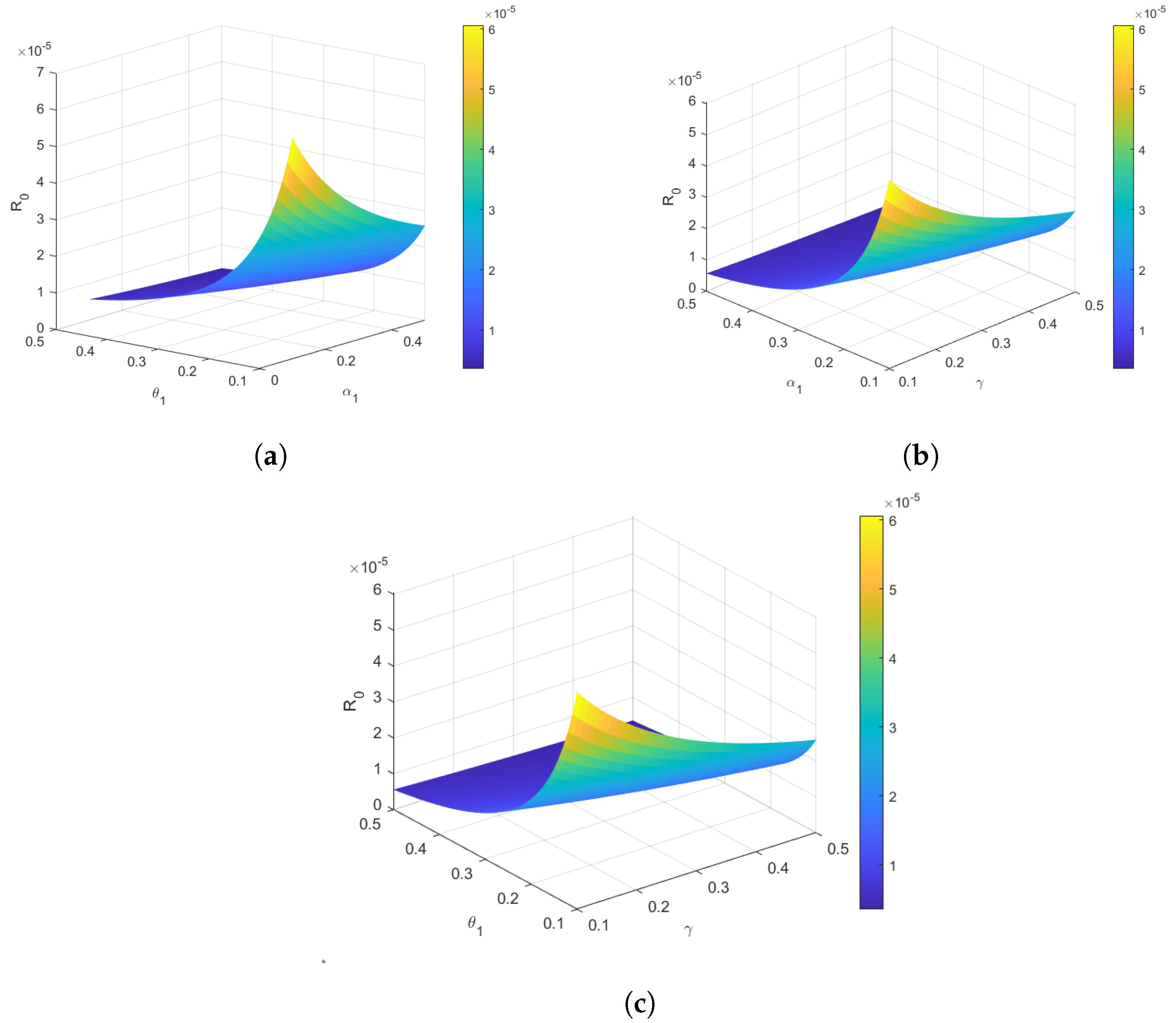
4.3. Reproduction Number $\left(R_0\right)$

To calculate the basic reproduction number for this model, we need to determine the expected number of secondary infections caused by one infected individual in a completely susceptible population. The derivation of $R_0$ involves finding the spectral radius of the next-generation matrix (NGM), which is a matrix that describes the expected number of secondary infections caused by each compartment. The NGM for this model is

$$\mathcal{F}=\left(\begin{array}{ccccc}\frac{\beta S}{\gamma +{\omega }_1}& 0& 0& 0& 0\\ \\ 0& 0& 0& 0& 0\\ \\ \frac{\beta S}{\gamma +{\omega }_1}& 0& \frac{\beta S}{\gamma +{\theta }_1+{\alpha }_1}& 0& 0\\ \\ 0& 0& \frac{{\theta }_{1}I}{\gamma +{\gamma }^2}& 0& 0\\ \\ 0& 0& \frac{{\alpha }_{1}I+{\alpha }_{2}Q}{\gamma }& 0& 0\end{array}\right)$$

Next, we find the spectral radius of this matrix where we need to find the eigenvalues and choose the one with the largest absolute value. Thus, we have the eigenvalues as

$${\lambda }_1=0,{\lambda }_2=\frac{\beta S}{\gamma +{\omega }_1},{\lambda }_3=\frac{\beta S}{\gamma +{\theta }_1+{\alpha }_1},{\lambda }_4=0,{\lambda }_5=0$$

The spectral radius of the NGM, which represents the basic reproduction number $R_0$ for the SVIQR model, is given by

$$\rho \left(\mathcal{F}\right)=max\left\{\mid {\lambda }_2\mid ,\mid {\lambda }_3\mid \right\}=max\left\{\left|\frac{\beta S}{\gamma +{\omega }_1}\right|,\left|\frac{\beta S}{\gamma +{\theta }_1+{\alpha }_1}\right|\right\}=\frac{\beta S}{\gamma +{\theta }_1+{\alpha }_1},{\omega }_1>{\theta }_1+{\alpha }_1$$

Hence,

$$R_0=\frac{\beta S}{\gamma +{\theta }_1+{\alpha }_1}.$$

(19)

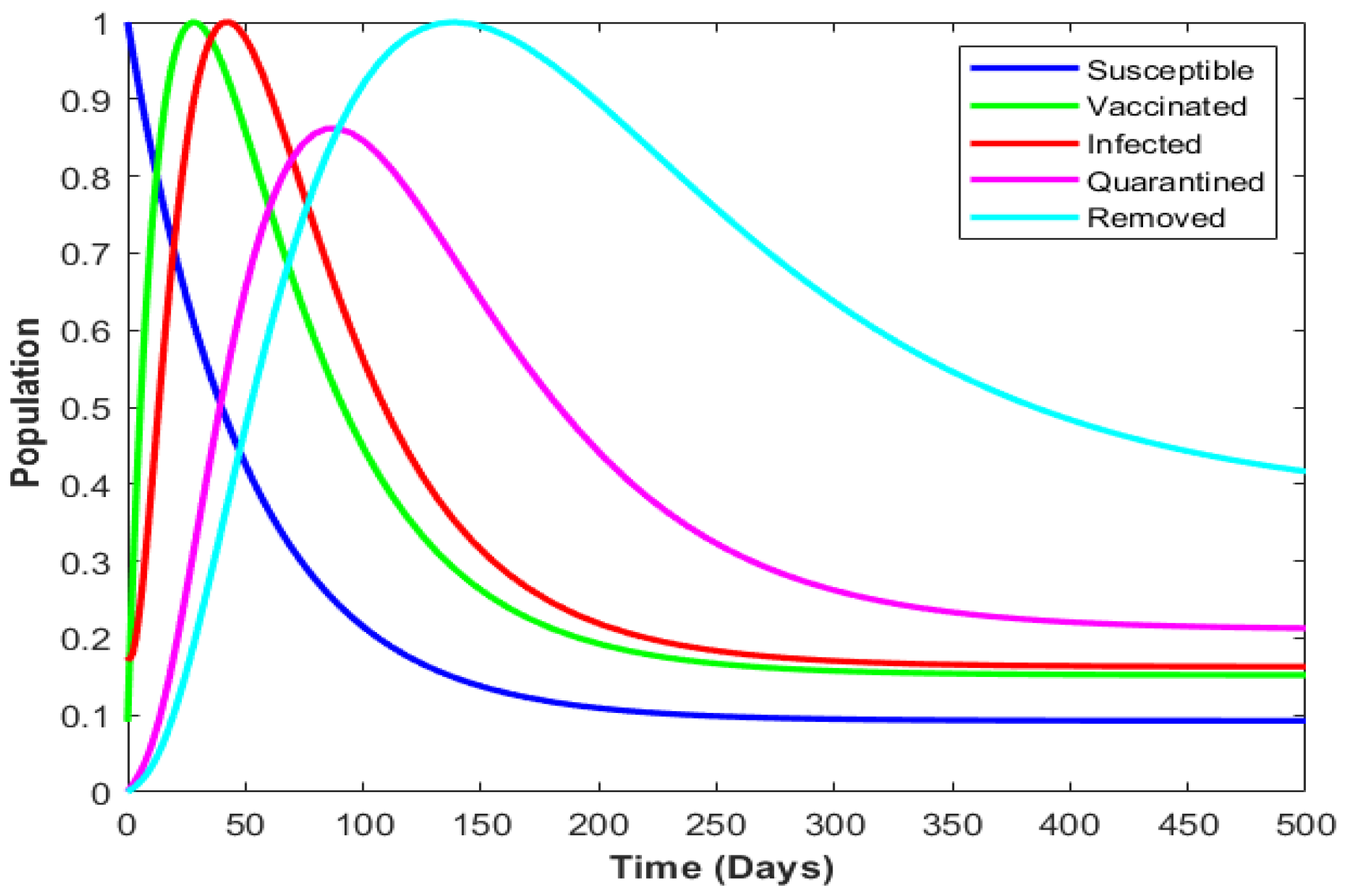
4.4. Numerical Illustration

We display the model behaviour for each compartment, and to further understand the contributions of the parameters on $R_0$, we shall perform the sensitivity analysis.

Figure 4 shows the behaviour of individuals within the population. It shows that most of the population is in the susceptible compartment, meaning they have not been exposed to the disease and are susceptible to infection. By considering the susceptible curve, it indicates that, as time progresses, the number of infected individuals increases as the disease spreads from person to person. This increase in the number of infected individuals leads to a decrease in the number of susceptible individuals as some people become infected and move from the susceptible compartment to the infected compartment. Eventually, the number of infected individuals reaches a peak and begins to decline as some individuals recover from the disease or die. As the number of infected individuals decreases, the number of removed individuals (those who have recovered from the disease or died) increases. In addition, the result also shows that, as the number of vaccinated individuals increases over time, there is a slow spread of the disease, which therefore reduces the number of susceptible individuals. From a biological perspective, this result shows how vaccination can be an effective strategy for reducing the spread of infectious diseases. By increasing the number of vaccinated individuals, we can reduce the number of susceptible individuals and slow the spread of the disease. Furthermore, it also suggests how the number of infected individuals can peak and decline over time as individuals recover from the disease or die.

Next, we plot the reproduction number against the dependent parameters to understand how the $R_0$ changes with a change in parameter values. The output displayed in Figure 5 shows how $R_0$ varies with different values of $[\gamma ,{\theta }_1,{\alpha }_1]$. As the value of these parameters increases, the transmission potential of the disease decreases, which leads to a lower value of $R_0$. The result exhibits a curve that starts high at low values of the parameters, and then gradually decreases as the parameter increases. This behaviour of the curve can be interpreted as a trade-off between the transmission potential of the disease and the ability of the population to mount an immune response. At low values of $[\gamma ,{\theta }_1,{\alpha }_1]$, the transmission potential is high, but the population has a weak immune response, so $R_0$ is high. Similarly, at high values of $[\gamma ,{\theta }_1,{\alpha }_1]$, the transmission potential is low, which implies that the population has a strong immune response, and therefore $R_0$ will be low. Hence, the minimum value of $R_0$ would correspond to the optimal balance between transmission potential and immune response.

Figure 5 shows the relationship between the reproduction number $\left(R_0\right)$ and the transmission rate ($\beta$) for different values of the recovery rate ($\gamma$), quarantine rate $\left({\theta }_1\right)$, and quarantine recovery rate $\left({\alpha }_1\right)$. The result shows that $R_0$ decreases with $\gamma$, ${\theta }_1$, and ${\alpha }_1$. In addition, it shows that the effect of ${\alpha }_1$ on $R_0$ is more pronounced at lower values of $\gamma$ and ${\theta }_1$. This implies that when $\gamma$ and ${\theta }_1$ are low, infected individuals are more likely to remain infectious and transmit the disease.

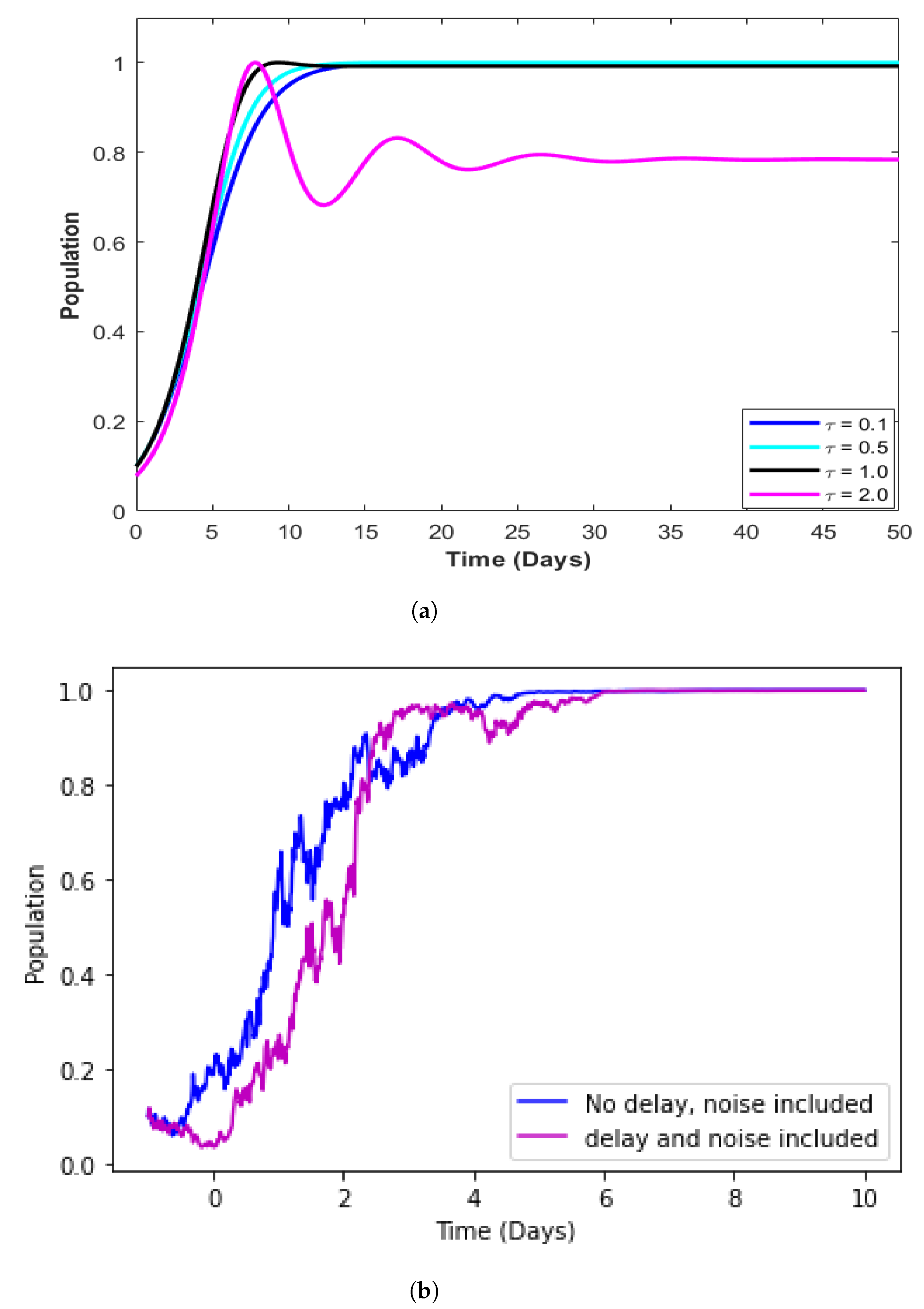
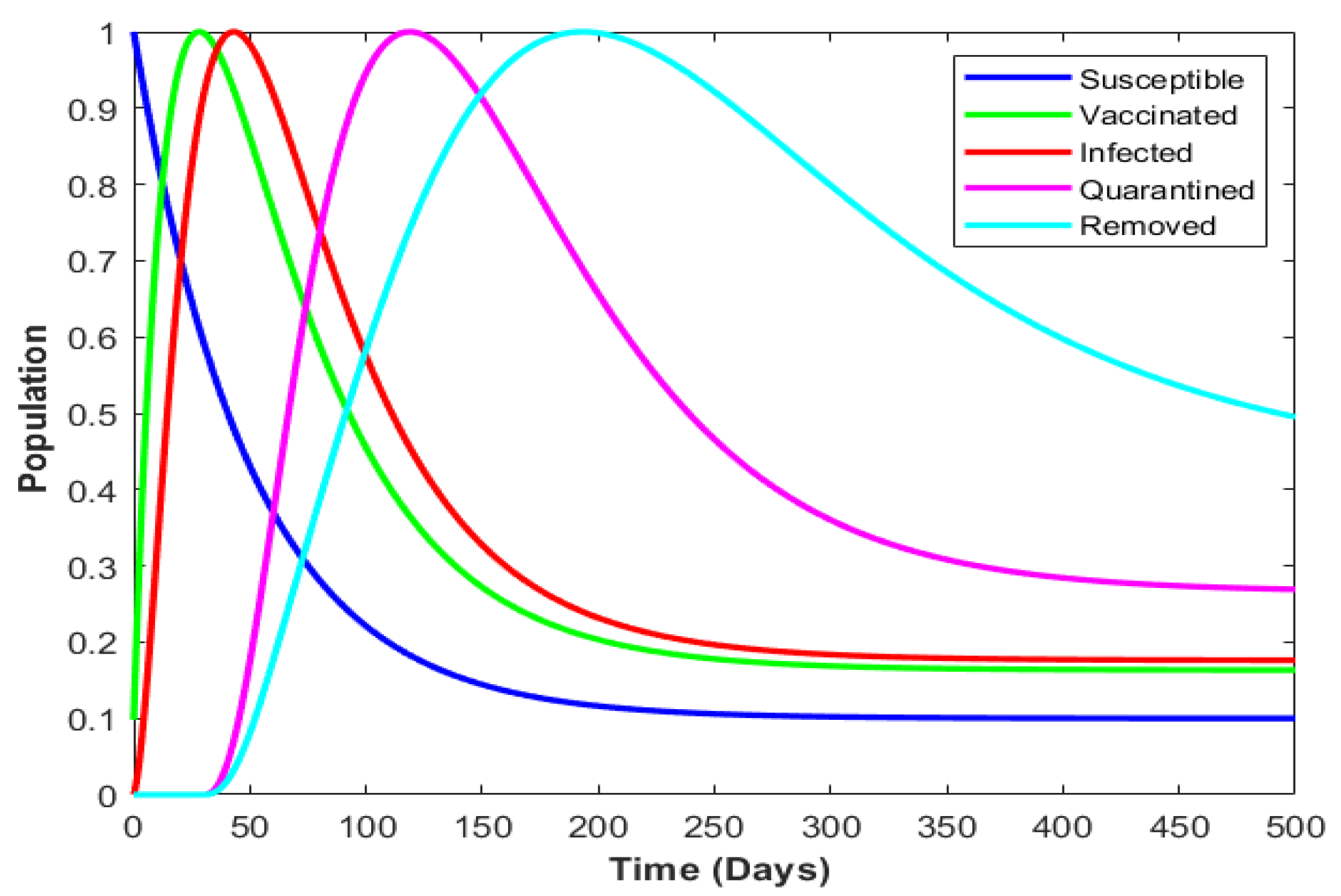
4.5. Model with Incorporated Delay

Here, we present the modification of this model to incorporate the time delay with the assumption that it takes a time period for the population to move from one compartment to the other. Hence, a modified version of (16), is given as

$$\begin{array}{cc}\hfill \frac{dS}{dt}& =\mu -\beta S(t-\tau )I(t-\tau )-(\gamma +{\omega }_1)S\left(t\right)\hfill \\ \hfill \frac{dV}{dt}& ={\omega }_{1}S\left(t\right)-\gamma V\left(t\right)\hfill \\ \hfill \frac{dI}{dt}& =\beta S(t-\tau )I(t-\tau )-(\gamma +{\theta }_1+{\alpha }_1)I\left(t\right)\hfill \\ \hfill \frac{dQ}{dt}& ={\theta }_{1}I(t-\tau )-(\gamma +{\alpha }_2)Q\left(t\right)\hfill \\ \hfill \frac{dR}{dt}& ={\alpha }_{1}I(t-\tau )-\gamma R\left(t\right)+{\alpha }_{2}Q(t-\tau )\hfill \end{array}$$

(20)

In the model (20), we have added a time delay $\tau$ to the terms involving the past values of S, I, and Q. The time delay is introduced to account for the fact that there is a lag between the time a person is infected with the disease and the time they become infectious. The delay also allows for the time it takes for an infected person to seek treatment and be moved to a quarantine centre. The modified model for the susceptible population includes a delay term $\beta S(t-\tau )I(t-\tau )$, which accounts for the time delay between the time an individual becomes infected and the time they become infectious. The recovered populations also include delay term ${\alpha }_{1}I(t-\tau )$, which represents the delay between the time an individual becomes infected and the time they recover. ${\theta }_{1}I(t-\tau )$ accounts for the delay between the time an individual is diagnosed with the disease and the time they are quarantined. The vaccinated population does not include a delay term, since vaccination is assumed to take effect immediately. Additionally, it is important to note that the choice of time delays depends on the specific disease and its transmission dynamics, and may require careful analysis or calibration to obtain accurate results. Additionally, incorporating time delays can make the model more complex and may require additional assumptions or parameters.

By comparing the output of Figure 4 with the result obtained in Figure 6, it could be observed that the delay has a significant impact on the behaviour of the system. In the model which does not incorporate any delay, the epidemic peaks rapidly and then gradually declines as the population becomes immune. The overall duration of the epidemic is relatively short, and the peak of the epidemic occurs at a relatively early time point. In contrast, the model which incorporates a delay in the transmission of the disease shows that the epidemic peak is delayed, and the epidemic lasts for a longer time. This delay is due to the time required for individuals to become infectious after being exposed to the disease. As a result, the epidemic spreads more slowly and gradually, and the peak of the epidemic occurs at a later time point. Therefore, we can conclude that incorporating delay in the transmission of the disease has a significant impact on the behaviour of the epidemic and can lead to different outcomes compared to a system without delay.

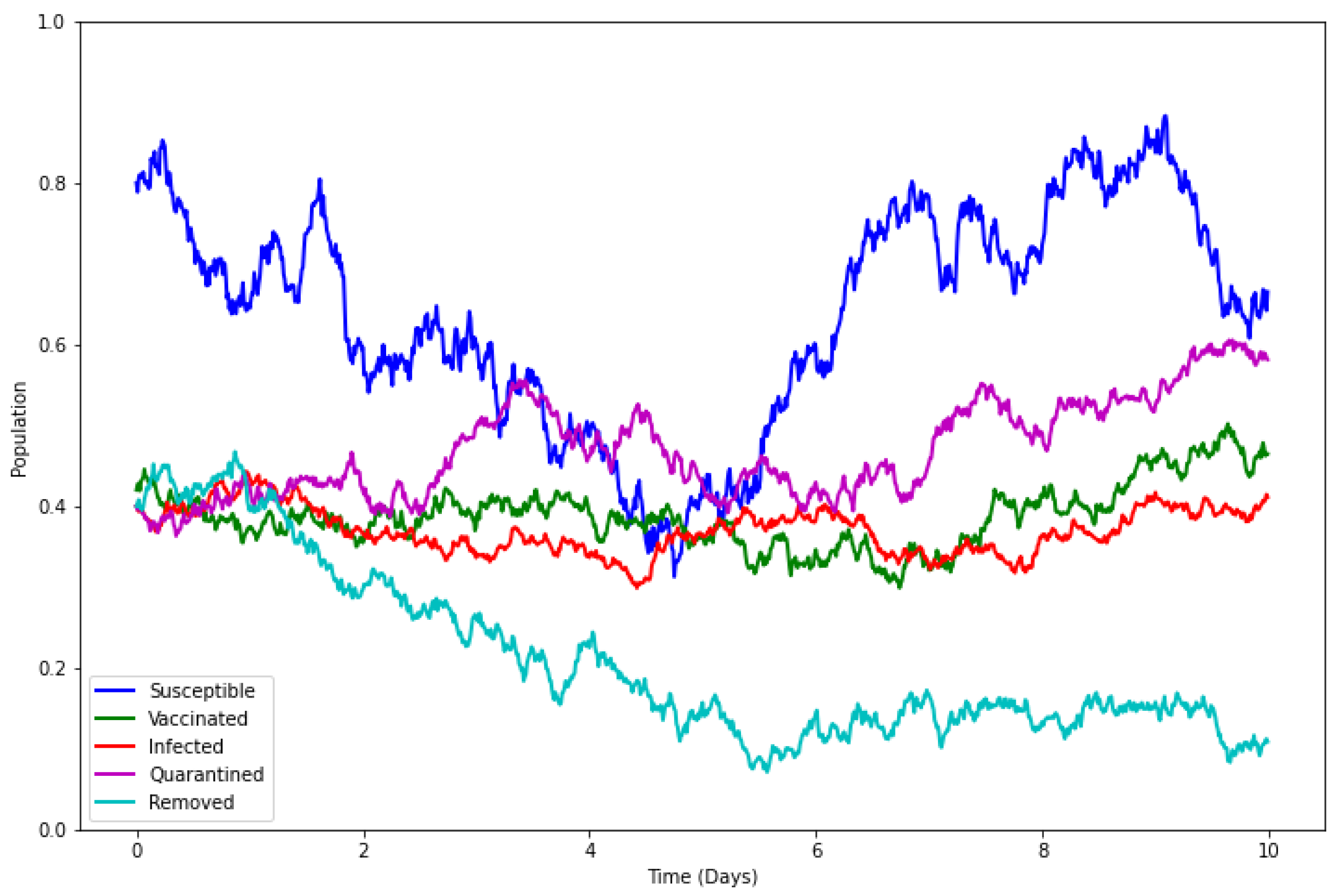
4.6. Model with Incorporated Delay and Additive Noise

The idea of incorporating noise into the system is born from the understanding that many real-world systems exhibit complex behaviour and are inherently noisy, with many exhibiting stochastic behaviour due to the presence of random fluctuations. In infectious disease models, the spread of disease is influenced by a multitude of factors that are difficult to model precisely. To account for some of the uncertainty in the system, noise can be added to the model. Moreover, many of the parameters in infectious disease models are uncertain or difficult to estimate precisely, adding further uncertainty to the model. By adding noise to the model, this uncertainty can be accounted for, resulting in a more realistic representation of the system. Additionally, non-linear dynamics can also contribute to the complexity of the system, even in the absence of external noise. The interactions between the various components of the system can give rise to hidden patterns and structures that may be difficult to discern otherwise. Hence, adding noise to the model can reveal these patterns and structures, allowing for a deeper understanding of the system. However, there are some challenges in adding noise to a model as there could be difficulty in determining the appropriate level of noise to add without overfitting or underfitting the data. Additionally, the choice of noise distribution can also have an impact on the model results. Therefore, when adding noise to infectious disease models, it is important to consider the characteristics of the disease being modelled and the specific research question being addressed. The type of disease, the available data, and the research objectives all play a role in determining the appropriate level and type of noise to incorporate into the model. Here, we are not looking into a specific dataset and we will only add a sample representation of noise into our system to show how the system behaviour changes when noise is included. Hence, we will represent our model as

$$\begin{array}{cc}\hfill \frac{dS}{dt}& =\mu -\beta S(t-\tau )I(t-\tau )-(\gamma +{\omega }_1)S\left(t\right)+{\sigma }_{S}d{W}_t\hfill \\ \hfill \frac{dV}{dt}& ={\omega }_{1}S\left(t\right)-\gamma V\left(t\right)+{\sigma }_{V}d{W}_t\hfill \\ \hfill \frac{dI}{dt}& =\beta S(t-\tau )I(t-\tau )-(\gamma +{\theta }_1+{\alpha }_1)I\left(t\right)+{\sigma }_{I}d{W}_t\hfill \\ \hfill \frac{dQ}{dt}& ={\theta }_{1}I(t-\tau )-(\gamma +{\alpha }_2)Q\left(t\right)+{\sigma }_{Q}d{W}_t\hfill \\ \hfill \frac{dR}{dt}& ={\alpha }_{1}I(t-\tau )-\gamma R\left(t\right)+{\alpha }_{2}Q(t-\tau )+{\sigma }_{R}d{W}_t\hfill \end{array}$$

(21)

${\sigma }_{S,V,I,Q,R}$ represent the noise associated to each model category. The assumption adopted here is that there is a level of uncertainty in the spread of the diseases and each compartment does exhibit random behaviour. A biological justification for noise inclusion in vaccination could be attributed to the existing knowledge that the efficacy of vaccines could vary based on factors such as the age and health status of the individual, the timing and number of vaccine doses, and the prevalence of different strains of the disease, etc. Thus, including noise in the vaccinated compartment $V\left(t\right)$ can help account for this uncertainty and provide a more realistic representation of the effects of vaccination on the spread of the disease. A similar argument can be generated for other compartments depending on the type of disease under consideration. Figure 7 displays the behaviour of the model with the noise. We could note that without the noise term, the model would be deterministic and assume that all individuals follow the same path of infection and recovery. However, in reality, there are always variations and uncertainties in how individuals are infected, vaccinated, or recover. The result here, therefore, captures the level of randomness exhibited in the system. Also, the result of the inclusion of noise in the model allows for the assessment of the variability in the predicted outcomes of the model, which can provide valuable insights into the robustness of the system and help identify areas of improvement for disease control measures.

5. Conclusions

Mathematical models have played a crucial role in the understanding of various biosystems. However, classical approaches based on ordinary differential equations (ODEs), delay differential equations (DDEs), or stochastic differential equations (SDEs) may not fully capture the real-life scenarios of these systems. Thus, the need arises for a more comprehensive approach that combines the features of these classical approaches, and this leads to the development of Stochastic Delay Differential Equations (SDDEs). In this work, we have investigated the application of SDDE-based models in understanding the behaviour of biosystems, particularly in epidemiology. We have presented a numerical technique for solving the model and shown that the SDDEs provide a more robust representation of real-life scenarios. The analysis of the quantitative and qualitative role of delay and noise reveals their significant influence on the overall behaviour of the system. The inclusion of delay terms in the model helps to capture the dynamics of the system, particularly in cases where there is a time lag between the infection and the manifestation of symptoms or the recovery process.

Similarly, the incorporation of stochasticity accounts for the uncertainty that arises in real-life scenarios and provides a more realistic representation of the system. We have presented numerical simulations to illustrate the robustness of the model, and the results suggest that the SDDEs provide a richer representation of many biological systems. Furthermore, the effects of delay and noise on the system have been investigated, and our results show that both delay and noise significantly impact the system’s behaviour. Delay leads to oscillatory behaviour in the system, and the amplitude of the oscillations depends on the size of the delay. On the other hand, the stochasticity introduced by noise leads to fluctuations in the system, and the size of the fluctuations depends on the strength of the noise. The combined effect of delay and noise leads to complex behaviour in the system, with a greater degree of variability and unpredictability than in deterministic systems.

Hence, the model devised in this study stands poised to significantly enhance our understanding of biosystem dynamics, with a particular focus on epidemiology. The utilisation of SDDE-based models offers a substantial leap towards crafting a more resilient representation of real-world scenarios by adeptly encompassing the dual factors of delay and stochasticity. Our numerical simulations robustly affirm that the model not only furnishes precise and efficient solutions but also holds substantial potential in predicting the intricate behaviours exhibited by biological systems. Furthermore, the insights garnered from this model can be instrumental in advancing the development of intervention strategies for combating diseases, thereby fortifying our ability to safeguard public health.

For future research directions, a pivotal area of exploration is the development of robust parameter estimation techniques tailored specifically for SDDEs. The accurate determination of model parameters from empirical data is critical for the practical application of SDDEs in epidemiology and other fields. Therefore, innovative approaches and methodologies for estimating these parameters will undoubtedly contribute to the model’s refinement and its ability to address real-world challenges effectively. In addition, we acknowledge that, in more practical scenarios, individual variables may indeed have different time delays. Future extensions of our work would be to explore the variations in delay values to provide a more nuanced understanding of the system’s behaviours.

References

1. Kammegne, B.; Oshinubi, K.; Babasola, O.; Peter, O.J.; Longe, O.B.; Ogunrinde, R.B.; Titiloye, E.O.; Abah, R.T.; Demongeot, J. Mathematical Modelling of the Spatial Distribution of a COVID-19 Outbreak with Vaccination Using Diffusion Equation. Pathogens 2023, 12, 88. [Google Scholar] [CrossRef] [PubMed]
2. Oshinubi, K.; Peter, O.J.; Addai, E.; Mwizerwa, E.; Babasola, O.; Nwabufo, I.V.; Sane, I.; Adam, U.M.; Adeniji, A.; Agbaje, J.O. Mathematical Modelling of Tuberculosis Outbreak in an East African Country Incorporating Vaccination and Treatment. Computation 2023, 11, 143. [Google Scholar] [CrossRef]
3. Buckwar, E. Introduction to the numerical analysis of stochastic delay differential equations. J. Comput. Appl. Math. 2000, 125, 297–307. [Google Scholar] [CrossRef]
4. Kloeden, P.E.; Platen, E. A survey of numerical methods for stochastic differential equations. Stoch. Hydrol. Hydraul. 1989, 3, 155–178. [Google Scholar] [CrossRef]
5. Higham, D.J.; Mao, X.; Yuan, C. Almost sure and moment exponential stability in the numerical simulation of stochastic differential equations. SIAM J. Numer. Anal. 2007, 45, 592–609. [Google Scholar] [CrossRef]
6. Mao, X. Robustness of exponential stability of stochastic differential delay equations. IEEE Trans. Autom. Control 1996, 41, 442–447. [Google Scholar] [CrossRef]
7. Bayram, M.; Partal, T.; Orucova Buyukoz, G. Numerical methods for simulation of stochastic differential equations. Adv. Differ. Equ. 2018, 2018, 17. [Google Scholar] [CrossRef]
8. Akutsah, F.; Mebawondu, A.A.; Babasola, O.; Pillay, P.; Narain, O.K. D-Iterative Method for Solving A Delay Differential Equation and a Two-Point Second-Order Boundary Value Problems in Banach Spaces. Aust. J. Math. Anal. Appl. 2022, 19, 6. [Google Scholar]
9. Rihan, F.A. Delay Differential Equations and Applications to Biology; Springer: Berlin/Heidelberg, Germany, 2021; pp. 123–141. [Google Scholar]
10. Bocharov, G.A.; Rihan, F.A. Numerical modelling in biosciences using delay differential equations. J. Comput. Appl. Math. 2000, 125, 183–199. [Google Scholar] [CrossRef]
11. Guillouzic, S.; L’Heureux, I.; Longtin, A. Small delay approximation of stochastic delay differential equations. Phys. Rev. E 1999, 59, 3970. [Google Scholar] [CrossRef]
12. Ivanov, A.; Kazmerchuk, Y.; Swishchuk, A. Theory, stochastic stability and applications of stochastic delay differential equations: A survey of results. Differ. Equ. Dynam. Syst. 2003, 11, 55–115. [Google Scholar]
13. Cooke, K.L.; Grossman, Z. Discrete delay, distributed delay and stability switches. J. Math. Anal. Appl. 1982, 86, 592–627. [Google Scholar] [CrossRef]
14. Murray, J.D. Mathematical Biology: I. An Introduction; Springer: Berlin/Heidelberg, Germany, 2002. [Google Scholar]
15. Benth, F.E.; Di Nunno, G.; Lindstrom, T.; Øksendal, B.; Zhang, T. Stochastic Analysis and Applications: The Abel Symposium 2005; Springer Science & Business Media: Berlin, Germany, 2007; Volume 2. [Google Scholar]
16. Milstein, G.N. Numerical Integration of Stochastic Differential Equations; Springer Science & Business Media: Berlin, Germany, 1994; Volume 313. [Google Scholar]
17. Kloeden, P.E.; Platen, E.; Kloeden, P.E.; Platen, E. Stochastic Differential Equations; Springer: Berlin/Heidelberg, Germany, 1992. [Google Scholar]
18. Saito, Y. Stability analysis of numerical methods for stochastic systems with additive noise. Rev. Econ. Inf. Stud 2008, 8, 119–123. [Google Scholar]
19. Mil’shtejn, G. Approximate integration of stochastic differential equations. Theory Probab. Its Appl. 1975, 19, 557–562. [Google Scholar] [CrossRef]
20. May, R.M. Simple mathematical models with very complicated dynamics. Nature 1976, 261, 459–467. [Google Scholar] [CrossRef] [PubMed]
21. Hutchinson, G.E. Circular causal systems in ecology. Ann. N. Y. Acad. Sci 1948, 50, 221–246. [Google Scholar] [CrossRef]
22. Golec, J.; Sathananthan, S. Stability analysis of a stochastic logistic model. Math. Comput. Model. 2003, 38, 585–593. [Google Scholar] [CrossRef]
23. Silva, C.J.; Maurer, H.; Torres, D.F. Optimal control of a Tuberculosis model with state and control delays. Math. Biosci. Eng. 2016, 14, 321–337. [Google Scholar] [CrossRef]
24. Yang, H.; Wang, Y.; Kundu, S.; Song, Z.; Zhang, Z. Dynamics of an SIR epidemic model incorporating time delay and convex incidence rate. Results Phys. 2022, 32, 105025. [Google Scholar] [CrossRef]
25. Babasola, O.; Kayode, O.; Peter, O.J.; Onwuegbuche, F.C.; Oguntolu, F.A. Time-delayed modelling of the COVID-19 dynamics with a convex incidence rate. Inform. Med. Unlocked 2022, 35, 101124. [Google Scholar] [CrossRef]
26. Tipsri, S.; Chinviriyasit, W. The effect of time delay on the dynamics of an SEIR model with nonlinear incidence. Chaos Solitons Fractals 2015, 75, 153–172. [Google Scholar] [CrossRef]
27. Culshaw, R.V.; Ruan, S. A delay-differential equation model of HIV infection of CD4+ T-cells. Math. Biosci. 2000, 165, 27–39. [Google Scholar] [CrossRef]
28. Nelson, P.W.; Perelson, A.S. Mathematical analysis of delay differential equation models of HIV-1 infection. Math. Biosci. 2002, 179, 73–94. [Google Scholar] [CrossRef] [PubMed]
29. Smith, D.L.; Battle, K.E.; Hay, S.I.; Barker, C.M.; Scott, T.W.; McKenzie, F.E. Ross, Macdonald, and a theory for the dynamics and control of mosquito-transmitted pathogens. PLoS Pathog. 2012, 8, e1002588. [Google Scholar] [CrossRef] [PubMed]
30. Aron, J.L.; May, R.M. The population dynamics of malaria. The Population Dynamics of Infectious Diseases: Theory and Applications; Springer: Boston, MA, USA, 1982; pp. 139–179. [Google Scholar]
31. Ruan, S.; Xiao, D.; Beier, J.C. On the delayed Ross–Macdonald model for malaria transmission. Bull. Math. Biol. 2008, 70, 1098–1114. [Google Scholar] [CrossRef]
32. Fosu, G.O.; Akweittey, E.; Adu-Sackey, A. Next-generation matrices and basic reproductive numbers for all phases of the Coronavirus disease. Open J. Math. Sci. 2020, 4, 261–272. [Google Scholar] [CrossRef]
Figure 1. Illustration of the effect of delay and noise in population dynamics. (a) Logistic equation with varying delay for y 0 = 0.1 , r = 0.5 . (b) Logistic equation incorporated with noise y 0 = 0.1 , r = 0.5 , τ = 1 , and σ = 0.5 .
Appliedmath 03 00037 g001
Figure 2. Illustration of the effect of delay and noise in population dynamics. (a) SIR model without noise and delay with β = 0.5 , γ = 0.1 . (b) SIR model incorporated with noise and delay with β = 0.5 , γ = 0.1 , τ = 3 , σ S = σ I = σ R = 2 .
Appliedmath 03 00037 g002
Figure 3. Illustration of the effect of delay and noise in the malaria model. (a) Model without delay for m = 2 , a = 0.2 , b = 0.5 , c = 0.5 , r = 0.05 , μ = 0.05 . (b) SIR model incorporated with noise and delay where τ 1 = 15 , τ 2 = 9 , σ x = σ y = 1 .
Appliedmath 03 00037 g003
Figure 4. Result of the SVIQR model without incorporated delays for μ = 0.02 , β = 0.0001 , γ = 0.01 , ω 1 = 0.01 ,   θ 1 = 0.05 ,   α 1 = 0.03 , and α 2 = 0.01 .
Appliedmath 03 00037 g004
Figure 5. The sensitivity analysis of R 0 with respect to the recovery and quarantine rate. (a) R 0 dynamic with varying θ 1 and α 1 . (b) R 0 dynamic with varying α 1 and γ . (c) R 0 dynamic with varying θ 1 and γ .
Appliedmath 03 00037 g005
Figure 6. Result of the SVIQR model with incorporated delays for μ = 0.02 , β = 0.0001 , γ = 0.01 , ω 1 = 0.01 , θ 1 = 0.05 , α 1 = 0.03 ,   α 2 = 0.01 , and τ = 30 .
Appliedmath 03 00037 g006
Figure 7. Result of the SVIQR model with incorporated delays and added noise where μ = 0.02 , β = 0.0001 , γ = 0.01 , ω 1 = 0.01 , θ 1 = 0.05 , α 1 = 0.03 ,   α 2 = 0.01 , τ = 30 and σ S = σ V = σ I = σ Q = σ R = 5 .
Appliedmath 03 00037 g007