Abstract
The leftmost column entries of RNA arrays I and II count the RNA numbers that are related to RNA secondary structures from molecular biology. RNA secondary structures sometimes have mutations and wobble pairs. Mutations are random changes that occur in a structure, and wobble pairs are known as non-Watson–Crick base pairs. We used topics from RNA combinatorics and Riordan array theory to establish connections among combinatorial objects related to linear trees, lattice walks, and RNA arrays. In this paper, we establish interesting new explicit bijections (one-to-one correspondences) involving certain subclasses of linear trees, lattice walks, and RNA secondary structures. We provide an interesting generalized lattice walk interpretation of RNA array I. In addition, we provide a combinatorial interpretation of RNA array II as RNA secondary structures with bases and base-point mutations where ω of the structures contain wobble base pairs. We also establish an explicit bijection between RNA structures with mutations and wobble bases and a certain subclass of lattice walks.
MSC:
05A15; 05A19; 05C05; 05C81; 92D20
1. Introduction
RNA combinatorics is one of the mathematical fields used for RNA sequence analysis and prediction [1,2,3]. This relatively new field combines topics from molecular biology, enumerative combinatorics, and bioinformatics. In this paper, we will interpret and analyze RNA secondary structures using various combinatorial techniques such as analyzing RNA arrays as combinatorial matrices, manipulating generating functions, solving recurrence relations, counting certain linear trees and lattice walks, and establishing explicit bijections. The main motivation for the bijections is that the given combinatorial objects may provide insight into the prediction of optimal RNA secondary structures. These bijections will allow RNA researchers to find and model optimal folding patterns that otherwise would be hard to observe and discover. Finding optimal structures may lead to more biological functionality for certain RNAs. Note that no RNA secondary structure prediction or folding was performed for this paper. Evans [4] used lattice walks to predict optimal RNA secondary folds of microRNAs related to tumor growth and cancer. This paper contributes to the literature on finding bijections between various combinatorial objects and RNA structures. See the following references [1,2,5,6,7,8,9,10] for other bijections between certain trees and RNA secondary structures.
Before we move on to the main results of the paper, we introduce Ribonucleic Acid (RNA) structures, RNA arrays, and the combinatorial objects presented in this paper. RNA plays a vital role in biological processes such as coding, decoding, regulation, and the expression of genes [11]. A single-stranded RNA molecule consists of a sequence of four nucleotides or bases, namely Adenine (A), Cytosine (C), Guanine (G), and Uracil (U). A sequence can be considered as a string of letters defined over where A linear RNA sequence of such bases is a one-dimensional structure called a primary structure. The RNA sequence in Figure 1 is an example of a specific one-dimensional structure.

Figure 1.
Primary RNA Structure.
When RNA molecules fold onto themselves, some nucleotides form base pairs through the creation of hydrogen bonds between complementary bases, where A pairs with U, U pairs with A, G pairs with C, and C pairs with G. These pairings are identified as Watson–Crick base pairs and this folding creates a two-dimensional structure. Uncommon cases where G pairs with U and U pairs with G are identified as non-Watson–Crick base pairs, called wobble pairs. The presence of GU (or UG) pairs occurs in the region of electronegative potential, which is proposed as the recognition site for the binding of metal ions and other positively charged ligands [12]. Molecules formed by the two-dimensional folding of RNA molecules are known as secondary structures. Those formed through the three-dimensional folding of RNA molecules are known as tertiary structures. For more information on RNA secondary structures and molecular biology, see the following references [11,13]. Note that if the nucleotide Uracil (U) is replaced by the nucleotide Thymine (T), then from the four nucleotides we obtain a Deoxyribonucleic Acid (DNA) molecule. DNA molecules are only mentioned in Section 5.
There are various ways to visually represent RNA secondary structures, such as biplanar graphs, arc diagrams, conventional diagrams, bracket notation, and tree representations [14]. As an example of arc diagrams, which are used most often throughout this paper, we start with the primary structure given above in Figure 1. A primary structure is first written along a horizontal line as depicted in Figure 1. Base pairs are represented as non-intersecting chords to form secondary structures. Figure 2 shows examples of two-dimensional RNA secondary structures represented by (a) non-intersecting arc diagrams and a conventional representation where, in (b), the stems are regions of stacked base pairs and the loops are identified as gaps between the stems. RNA secondary structures and RNA sequences are used interchangeably in this paper. Note that pseudoknot RNA secondary structures represented by intersecting arc diagrams are not considered in this paper.
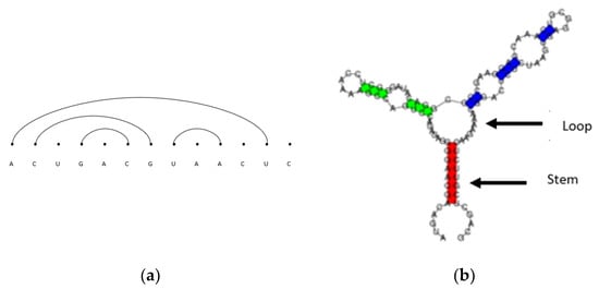
Figure 2.
(a) An arc diagram representation of a longer RNA secondary structure; (b) a conventional diagram representation of RNA secondary structure.
In a non-biological context, secondary structures are of vital consideration in RNA computing, prediction, and analysis since the pattern of base pairs ultimately determine the overall structure of a molecule. Knowing a biomolecule’s precise structure is one of the foremost goals of molecular biology [15]. It is the structure that determines the molecule’s function. Moreover, determining the three-dimensional tertiary structure of RNA has proved to be more difficult [16]. Such a situation has created an intense search for secondary structure prediction methods: methods that can predict the optimal secondary structure of a molecule based on the folding of its one-dimensional primary structure.
We now consider the two infinite lower triangular arrays and —which we call RNA arrays I and II, respectively—that are associated with RNA secondary structures. The first few entries are listed below in Figure 3. The leftmost column entries of the arrays count the sequence of integers {1, 1, 1, 2, 4, 8, 17, …} known as the RNA numbers [17]. Focusing on the leftmost columns, note that the leading ‘1’ in the sequence is not included in . The RNA numbers are also called generalized Catalan numbers [17]. See the following references [18,19,20] for background information on the construction and development of and .

Figure 3.
RNA arrays I and II.
These two lower triangular RNA arrays (or combinatorial matrices) were first introduced by Nkwanta [18,19,20,21]. It is also known that the RNA arrays are proper Riordan arrays [18,19,20]. Riordan arrays form a special subset of infinite lower triangular arrays that are typically used as tools for proving combinatorial identities [22]. The definition of Riordan array is given in Section 4.1. The method used to produce combinatorial interpretations of Riordan arrays and to solve combinatorial recurrence relations related to Riordan arrays is called the Riordan matrix method. Some parts of the method are introduced in this paper. See [7,20,23] for more information on the Riordan matrix method.
We will now explore well-established explicit bijections between RNA secondary structures and the various combinatorial objects, as illustrated in Figure 4.
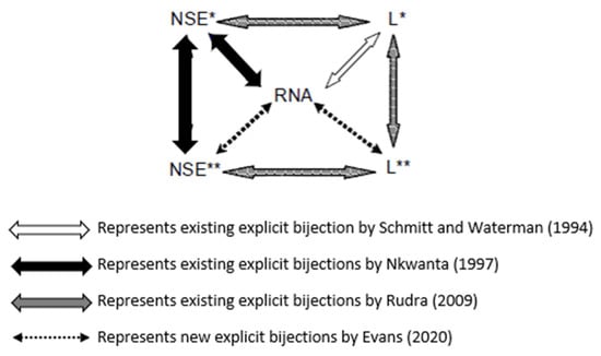
Figure 4.
Refs. [18,19,24,25] Connections among linear trees, lattice walks, and RNA secondary structures.
In 1994, Schmitt and Waterman [24] established an explicit bijection between the set of all secondary structures of a given length with a fixed number of base pairs and a particular set of plane trees. In 1997, Nkwanta [19] introduced a lattice walk interpretation of RNA array I, denoted by , by showing that the entries of the array count the number of a certain subset of lattice walks of length ending at height , denoted by . Consequently, this led to establishing an explicit bijection between lattice walks and RNA secondary structures. Additionally, also in 1997, Nkwanta established another bijection between another subclass of unit-step lattice walks of length n ending at height denoted by and the lattice walks. The lattice walks were given as a combinatorial interpretation of RNA array II, denoted by . Then in 2009, motivated by Nkwanta and Schmitt and Waterman’s correspondences, Rudra [25] established an explicit bijection between the lattice walks and a certain subclass of linear trees denoted by . By establishing another subclass of linear trees denoted by , Rudra introduced an additional bijection between the lattice walks and linear trees. In addition, Rudra established a correspondence between linear trees and linear trees. In 2020, Evans [4] resolved two open problems presented by Rudra [25] by establishing explicit bijections among linear trees, lattice walks, and RNA secondary structures. See the following references [1,2,5,6,7,8,9,10] for other bijections between certain trees and RNA secondary structures. The motivation for the bijections is that the given combinatorial objects may provide insight into the prediction of RNA secondary structures. Note that no RNA secondary structure prediction or folding was performed in this paper.
This paper is organized as follows. In Section 2, a brief introduction describes the combinatorial objects presented in the paper. The new explicit bijections by Evans are proved in Section 3. The motivation for the bijections is that the lattice walks and/or linear trees may provide some insight into the folding (modeling) of RNA secondary structures [26]. In Section 4, we propose an interesting generalized interpretation of . We do this by taking -copies of , denoted by , and proving that the entries of the array count the number of -colored lattice walks, of length , ending at height . This result is not obvious and exhibits a nice pattern of the formation rules of the column entries of the higher dimensional arrays. In Section 5, we combinatorially interpret in terms of RNA base-point mutations and wobble base pairs. We denote as the number of RNA secondary structures of length with base-point mutations that have wobble base pairs. Since the entries of count lattice walks as well as RNA secondary structures with base-point mutations where of the structures contain wobble base pairs, a new explicit bijection is established between these two combinatorial structures. Recall that the definition of wobble base pairs is given earlier in this section. Mutations are defined later in Section 5. For more details on the new results presented in this paper, see reference [4].
2. Combinatorial Objects
2.1. RNA Secondary Structure
Schmitt and Waterman [24] presented the below definition of RNA secondary structure from a graph theoretic point of view.
Definition 1.
“A secondary structure of length is a simple graph on with vertices in and edges in , i.e., a set
of unordered pairs of elements of
that satisfies
- (a)
- degreefor,
- (b)
- if, then
- (c)
- if, whereand, andthen eitheror(wheredenotes the interval
An edge between vertices labeled and is defined as a base pair, and a vertex not adjacent to any edge is defined as an unpaired base. We visually represent these RNA secondary structures starting with the primary structure along a horizontal line and drawing edges as arcs in the upper half-plane. Condition (a) of the definition restricts a single base to pair with only one other base in the structure. Condition (b) guarantees that no two adjacent bases can pair. Condition (c) guarantees that no two arcs cross one another. In addition, if arc is nested in arc then These conditions align well with the Watson–Crick base pairing restrictions placed on an RNA molecule [3].
Let be the sequence of the number of secondary structures on denoted by
Thus, for and initial conditions , we have the following recurrence relation:
The generating function of (of the RNA numbers) is derived from the recurrence relation and given as
Proofs of the generating function and recurrence relations can be found in the following references [27,28].
2.2. Linear Trees
Below is the definition of the linear trees mentioned in this paper.
Definition 2.
[24] A linear tree is defined as a rooted tree with a linear ordering on the set of children of each vertex in the tree. In a linear tree, the number of edges from the current vertex to the root is called the level of . Each vertex has a level from 0 to where
represents the height of the rooted tree. There is exactly one vertex at level 0, which is the root. All vertices adjacent to vertex
on a lower level are called the children of . A vertex is called terminal if it has no children and is called non-terminal otherwise. If vertex
immediately precedes vertex
on the path from the root to
, then
is the parent of
. Vertices that have the same parent vertex are identified as siblings. A linear tree will be depicted with the root at level 0 and with the children of level
arranged on level
. The trees are inverted (that is, flipped upside down) and the root at level 0 is the highest level.
Let be the set of unlabeled linear trees with vertices, with of them being non-terminal. The exact formula for is given in [24] by
For example, Figure 5 shows the six members of the set .

Figure 5.
The set with five vertices, with three of them being non-terminal.
2.3. Lattice Walks
A lattice walk is a sequence of contiguous and reversible unit steps which traverses a d-dimensional integral lattice [18]. Most of the interpretations mentioned in this paper arise from the combinatorial objects called lattice walks: specifically, those walks that have the step directions of north, south, and east, respectively represented by the symbols N, S, and E. The N and S steps are the only reversible unit steps mentioned in this paper.
Definition 3.
[18] An NSE lattice walk is a sequence of adjoining unit steps that covers the two-dimensional integral lattice . An NSE lattice walk of length
and height
begins at (0, 0), remaining above the
-axis in the first quadrant. The step directions are: (0, 1) = N (North or up), (0, -1) = S (South or down), and (1, 0) = E (East or right). The length of each walk is the number of unit steps, and the height corresponds to the
-value at end-point (x, y).
An example of a NSE lattice walk is given below in Figure 6.

Figure 6.
NSE lattice walk: NEESEENEES of length 10 and height 0.
We put additional restrictions on the NSE lattice walks as given by Definition 3 to create the following walks that are also two-dimensional.
Definition 4.
[18,19,20] Let anddenote unit step NSE lattice walks, defined as follows:
- (a)
- are lattice walks that do not have consecutive pairs of N (north) and S (south) steps. For instance, the walk NEESENSEE is not an example of an walk.
- (b)
- are lattice walks that do not have consecutive pairs of S(south) and N(north) steps. For instance, the walk NEESNEES is not an example of an walk.
In the next section, we present explicit bijections among the combinatorial objects given in this section.
3. New Explicit Bijections
The following theorem gives a new explicit bijection between the set of lattice walks and a certain subset of RNA secondary structures.
Theorem 1.
There is an explicit bijection between the set of unit-step lattice walks of length ending at height and the set of RNA secondary structures of length .
Proof.
To establish the required correspondence, let be an arbitrary unit-step lattice walk of length ending at height . Since is an lattice walk, there are no SN steps in the walk. To form an RNA secondary structure of length , we use the rules described below.
Given , insert an additional th step at the end of the walk, restricting this step to an E step only. Beginning with the th step and moving left through the sequence, we move every E step we encounter positions to the left, where is the number of consecutive S steps directly to the left of the E step. E steps can only move if there is a S step to the left of it. Note that some E steps will be fixed depending upon the walk structure of (i.e., if there are no S steps to the left of the E step). In this construction: (1) Walks never go below the -axis; (2) there is no pairing between S and N steps; and (3) since walks are of height k = 0, there is always an E step or a sequence of E steps between consecutive N and S steps.
Next, we form an RNA secondary structure of length and height k = 0. We label corresponding NS steps as th base pairs and they become bonded bases of RNA following the Watson–Crick base pairing rules. We label E steps as th unpaired bases. Additionally, note that the nested innermost NS steps are paired first to avoid base pairs from crossing. Then, we number the positions of the steps of from one to and pair position with position to form the base pairs . Recall that the E steps are unpaired bases. Via the bijection between the walks and RNA secondary structures [19], we obtain a walk of length The trivial case of the correspondence is when there are only E steps in the walk, so the appended step does not move left. Therefore, an RNA structure of length is formed. The correspondence is constructed, and reversing the process illustrated in Figure 7 produces the outline of the proof of the reverse map. As a consequence of the reverse map, by following the Watson–Crick base pairing rules and the way the lattice walk steps are assigned to a walk, no consecutive S and N steps are possible. We move through the example of reversing the steps as follows: let be an arbitrary RNA secondary structure of length and height . We write in its linear form as a sequence of bases, denoted by integers, increasing in order from left to right along a horizontal axis with bases. We identify paired and unpaired bases and arcs are drawn between paired bases. By the correspondence, if an arc links integers and with , we then label the th pairing members as (N,S) steps. If a base is unpaired, label the kth unpaired base as an E (east) step. Moving through the sequence from left to right, we move every E step we encounter positions to the right where is the number of consecutive S steps directly to the right of the E step. Lastly, we remove the right most E step resulting in an lattice walk of length at height . Thus, the correspondence is one-to-one, and the theorem is proved. □
As an example of the correspondence, consider the unit step walk of length. By the rules of the correspondence, a possible RNA secondary structure of length 16 is obtained in the following figure.
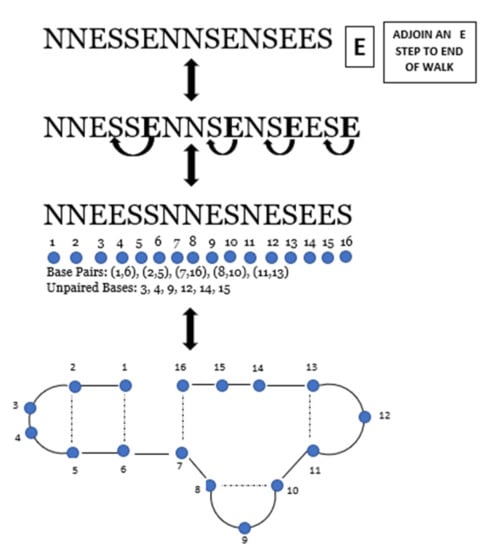
Figure 7.
One-to-one correspondence between and a possible RNA sequence. Dashed lines represent paired bases.
Now, before we move on to the next new theorem, we will discuss the labeling of the linear tree , which we now denote by . Recall that the linear tree was given earlier in Section 2.2. Thus, the linear tree is a modified version of described as follows. Each vertex has a level, ranging from 0 down to level , with exactly one root vertex, which is at level 0. All adjacent vertices differ by exactly one level and each vertex at level is adjacent to exactly one vertex at level h. are labeled linear trees with a linear ordering on the set of children of each vertex in the tree. Vertices are labeled consecutively by searching depth first from left to right, starting with 0 at the root. Vertices are labeled only when they are first encountered and last encountered, thus resulting in each vertex in a linear tree being labeled by two integers. However, there is an exception to the rules of labeling. Children with the same parent vertex will always have every other sibling labeled with one integer. The descriptions for terminal and non-terminal vertices are given in the proof for Theorem 2.
Recall that the notion of bijectivity is an equivalence relation on sets. Since there are explicit bijections between RNA secondary structures and linear trees, and between linear trees and linear trees, there exists an explicit bijection between RNA secondary structures and the set of linear trees, with , given by the following theorem.
Theorem 2.
For all there is an explicit bijection between the set of linear trees
with
vertices,
of which are non-terminal, and
of which are terminal vertices that are labeled by two consecutive integers and the set of RNA secondary structures
of length
that have
base pairs.
Proof.
Suppose and is a rooted labeled linear tree with vertices, of which are non-terminal, and of the terminal vertices are labeled by two consecutive integers. To establish the required correspondence, we begin by considering each vertex at level of , starting at level 0 and moving to the lowest level in the tree. We consider the following cases:
- (a)
- If the vertex at level is non-terminal, then the vertex remains unchanged.
- (b)
- If the vertex at level is terminal and
- (i)
- labeled with two consecutive integers, then a child vertex (terminal) is inserted at the endpoint. This new child will be on level
- (ii)
- labeled with one integer, then the child vertex remains unchanged, except in the case that the vertex is positioned between two vertices that are labeled by two integers, in which case the child vertex (terminal) is removed from in between the vertices. Note that this vertex will be labeled with one integer.
Next, after reconstructing the new linear tree by deleting and/or adding vertices, we remove all labels from . The linear tree receives new labeling rules by a depth-first search moving left to right around the tree. We relabel the vertices as they are encountered by consecutive integers (starting with 0 at the root); however, we label internal vertices only when they are first and last encountered. Note that these will be the non-terminal vertices that are labeled by two integers. Terminal vertices are labeled by one integer. As we leave the linear tree form, we now represent the tree as an RNA secondary structure. The resulting pairs of labels on the non-terminal vertices of the linear tree correspond to the paired bases of the structure. Following the Watson–Crick pairing rules, the unpaired labels on the terminal vertices of the linear tree are associated with the unpaired bases of a secondary structure.
The following properties are observed in the above construction: (i) The length of the RNA secondary structure is composed of all vertices of , in addition to all vertices that are labeled by two integers (paired integers). This includes non-terminal (internal) vertices and terminal vertices that are labeled by two consecutive integers. Therefore, we obtain an RNA secondary structure of length . (ii) The number of base pairs in the RNA secondary structure is composed of all internal vertices of , in addition to all terminal vertices that are labeled by two consecutive integers. Therefore, we obtain an RNA secondary structure that has base pairs. (iii) We also observe that the unpaired bases of the RNA secondary structure correspond to .
Therefore, an RNA secondary structure of length with base pairs is formed and denoted by ). The correspondence is constructed and reversible. Thus, the theorem is proved. □
As an example of the correspondence, consider for and as in Figure 8 below. To construct an RNA secondary structure, we consider each vertex at level of . Starting at the highest level 0 and moving to the lowest level:
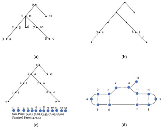
Figure 8.
(a) labeled linear tree. (b) By following the rules of the bijection, a new linear tree is formed by removing all labels, re-attaching the edge (1, 6) denoted by the dotted line to the end of old vertex (3, 4), and adding a new edge denoted by an edge with a tick mark to the end of old vertex (8, 9). (c) Follow the new labeling rules and number the vertices from one to thirteen and associate pairs and unpaired bases with a specific RNA structure. (d) RNA secondary structure (13, 5). Dashed lines represent paired bases.
- Level 0 has one non-terminal vertex 0 (the root), so according to the rules, the vertex remains unchanged.
- Level 1 has one non-terminal vertex (1, 11) and one terminal vertex (12) labeled with one integer. According to the rules of the bijection, both vertices remain unchanged.
- Level 2 has one terminal vertex (6) positioned between two vertices {(2, 5), (7, 10)} that are labeled by two integers; therefore, we remove the terminal vertex (6) from in between the vertices.
- Level 3 has two terminal vertices {(3, 4), (8, 9)}, both labeled with two consecutive integers, so we add a terminal vertex at the end of (3, 4) and at the end of (8, 9).
Next, starting with the root, we move around the tree starting with a depth-first search and relabel vertices using consecutive integers where only non-terminal (internal) vertices are labeled with two integers. Internal vertices are labeled as they are first and last encountered. We ignore the root as we move to form the secondary structure. As a result of relabeling the vertices, vertices labeled by two integers form the set of base pairs {(1, 12), (2, 6), (3, 5), (7, 11), (8, 10)} and vertices labeled by a single integer form the set of unpaired bases {4, 9, 13} for the secondary structure (13, 5) of length 13 with five base pairs.
We note when for we obtain which is the set of unlabeled linear trees that have vertices and of which are non-terminal.
4. Generalized Lattice Walk Interpretation of
A generalized interpretation of is presented in this section. We take higher ordered arrays of and prove that counts -colored lattice walks when . Recall that counts the lattice walks identified according to Definition 4(a). Note that the walks come in -colored E (east) steps. We first prove is a Riordan matrix. Then, we give a combinatorial interpretation of in Section 4.2.
4.1. Recursions for Generalized Array
Consider , the first few entries of which are given below.
here, we give an example for to show how the entries of are formed. We observe that the first column entry is computed by , and the leftmost column entry is computed by . See the following diagrams that illustrate the formation rules shown above, (a) 28, (b) 36.
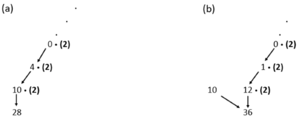
These patterns continue to form all of . In fact, the pattern continues for all of .
In general, the th entry of the array is formed and computed recursively using the following recursions. Let be the initial condition. Then, for , and
where if .
The leftmost column entries of are given by Equations (2) and (3) and produce the other column entries of . The Riordan matrix method will subsequently be used to prove the recursions.
From the recursions, we can derive explicit generating functions whose coefficients make up the column entries of . With these generating functions we can define as a Riordan matrix. The concept of a Riordan matrix was introduced in 1991 by Shapiro [29]. The definition is given below.
Definition 5.
An infinite matrix with complex entries
is called a Riordan array if the kth column satisfies
where corresponds to the leftmost column and the expression corresponds to the kth column, where
From Definition 5, if for g(z) and for , then the Riordan arrays are called proper Riordan arrays. A set of all proper Riordan arrays are Riordan matrices, and they form a group called the Riordan group [29].
Thus, the coefficients of the column-generating functions of the form make up the columns of . In this case, is an infinite lower triangular array, denoted as a pair .
The first few terms of the well-known Pascal triangle, shown below in lower triangular form and denoted by is an example of a typical Riordan matrix.
RNA arrays I and II are defined, respectively, as Riordan matrices by
where is the generating function given by Equation (1).
We now apply the Riordan matrix method to solve the recursion and generating functions associated with . According to the formation rules of given by Equation (3), the th column-generating function of the matrix is defined as
Solving for , we obtain
Then, by using the quadratic formula, solving in terms of and simplifying, becomes
Similarly, according to the formation rules of given by Equation (2), the leftmost column-generating function is defined as
Simplifying this equation and expressing in terms of produces
where is the generating function of the other array columns and is given by Equation (4). By substituting the value of rationalizing the denominator, and simplifying, we obtain
Now, let . Using Equations (4) and (6), we obtain explicit generating functions of given in pair form as the Riordan matrix.
Four remarks are now given for .
Remark 1.
is a Riordan matrix since is an element of the Riordan group, and we know by closure that is an element of the Riordan group. In addition, is a pseudo involution and an element of the Bell subgroup of the Riordan group. See, the references [29,30] for the definition of pseudo involution and Bell subgroup, respectively.
Remark 2.
is related to the Catalan-generating function [31], denoted below by The generalized Riordan form of in [30] is given as
where
is the RNA-generating function given by Equation (1),
However, the correct form is
Remark 3.
The expression
is known for [32]. It generalizes to
and can be shown to hold for
. That is,
Additionally, note that
and
generalize Equations (3) and (4), respectively.
Remark 4.
A generalized form of Equation (5) is given as
4.2. Combinatorial Interpretation of
Before proving Theorem 3 below, we define a generalization of the lattice walks. Recall that are the lattice walks given by Definition 4(a). Let denote the set of all -colored NSE* lattice walks of array , where , of length and height . We will prove later in this subsection. This array is a product of copies of , where each East(E) step is one of j colors. We start with examples of -colored lattice walks (see Figure 9 and Figure 10 below).

Figure 9.
All 10 lattice walks of entry of . Variation of arrows represent different colored E steps.
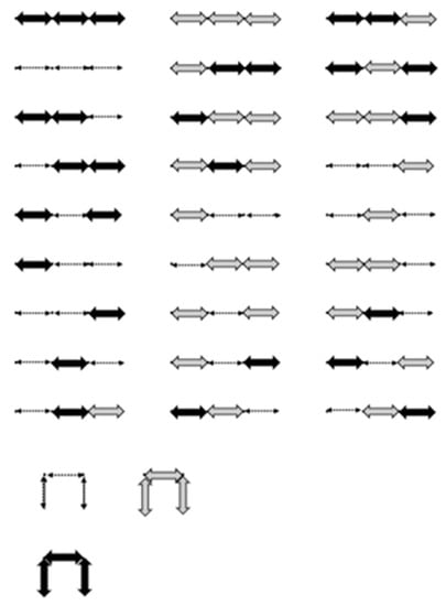
Figure 10.
All 30 lattice walks of entry of . Variation of arrows represent different colored E steps.
Note that we continue with the Riordan matrix method for proving combinatorial interpretations of Riordan arrays. Given Equations (2) and (3), we provide a combinatorial proof that counts -colored lattice walks of length and height of array .
Theorem 3.
Given the initial condition ,
, and
,
then satisfies the following recurrence relation where (a) is defined for the leftmost column of and (b) is defined for the other columns of :
- (a)
- (b)
Proof.
We start by proving (b). Suppose a -colored lattice walk of length and height for array is given. Then, to form a new walk of length and height , consider the following cases:
Case (i): If the given walk has length and height , then on the last step there is one choice for height (the N step). In this case, all walks whose last step is N are counted by .
Case (ii): If the given walk has length and height , then on the last step there is one choice for height (the E step). In this case, there are possible colored E steps. Thus, all walks whose last step is E are counted by .
Case (iii): If the given walk has length and height , then the last possible sequence of steps for height is ES (east, south steps). In this particular case, there are possible colored ES steps. Thus, all walks whose last consecutive sequence of steps is ES are counted by .
Case (iv): If we continue and have a walk of length and height , then the last possible sequence of steps for height (east, south m times). These sequences occur since there are no NS steps allowed. There are also possible colored sequences of steps. Here, all walks whose last sequence of steps is are counted by .
Applying the addition principle and multiplication rule concludes that recurrence relation (b) is proved. Recursion (a) is easy to prove by similar reasoning. □
5. RNA Interpretation of and Bijection
In this section, we give two RNA combinatorial interpretations of . One interpretation is given in terms of RNA secondary structures with mutations and wobble pairs, and the other is in terms of RNA secondary structures with mutations and structures with wobble pairs and non-wobble pairs. Before deriving the interpretations of , we define what we mean by RNA mutation.
In biology, mutations are defined as random changes/alternations in the genomes in a cell, either in DNA or RNA. Mutations occur due to exposure to ultraviolet (UV) light, replication errors, or the degradation of bonds in DNA. Alternations that happen during the DNA replication of a single nucleotide (base) where a base may be substituted, inserted, or deleted are defined as point mutations. The consequences of these mutations lead to protein composition, production, and functionality. Point mutations include several types [33]:
- (a)
- Substitution—when one or more nucleotides (bases) in the sequence are replaced by the same number of bases (for example, a cytosine substituted for an adenine).
- (b)
- Insertion—when one or more nucleotides (bases) are added to the sequence.
- (c)
- Deletion—when one or more nucleotides (bases) are removed from the sequence.
Figure 11 below shows an example of various point mutations of an RNA sequence, where each mutation is underlined and in bold print.

Figure 11.
Examples of point mutations in an RNA sequence.
5.1. RNA Mutations and Wobble Base Pairs
Recall that Rudra proposes an RNA combinatorial interpretation of in terms of RNA structures with mutations in [25]. We now propose, in this subsection, an RNA combinatorial interpretation of in terms of RNA structures with mutations where of the structures contain wobble base pairs. A combinatorial meaning of wobble base pairs is given in terms of arc diagrams. This is completed by labeling consecutive G and U base pairs as G–U pairs and U and G base pairs as U–G pairs. We call the G–U (U–G) pairs ‘wobble base pairs.’ Wobble base pairs are connected by arcs of consecutive base pairs at positions and of an RNA sequence. Recall that RNA sequences and RNA structures are used interchangeably. Wobble pairs are restricted to not allowing consecutive G–U (U–G) base pairs. This means there are no sequences with GUGU (UGUG, UGGU, GUUG) bases. Generally, we mention here that in the biological literature, wobble pairs are not necessarily labeled as G–U (U–G) pairs [34]. In this paper, base-point mutations are represented by ⊙ and restricted to the following conditions:
- (a)
- They do not occur under an arc of two paired bases
 .
. - (b)
- They do not occur as a point of a base pair
 .
. - (c)
- They do not occur to the right of any wobble base pairing, whether that pairing is isolated or nested under an additional base pair that is connected by an arc diagram
 .
.
Proposition 1 below gives a combinatorial interpretation of in terms of RNA secondary structures with mutations that contain wobble base pairs. See Figure 12 for an example where seven RNA sequences contain base-point mutations and wobble base pairs.

Figure 12.
RNA sequences with a length of five and one base-point mutation that contains sequences with wobble base pairs.
Proposition 1.
Given the initial conditions ,
, and
, for
and 0, satisfies the following recurrence relation for all column entries of except for the leftmost column
where
counts the number of RNA secondary structures of length
with
mutations that contain wobble pairs.
See Figure 13 below for an example of the construction of the seven sequences with base-point mutations and wobble base pairs given by Figure 12. By the recursion, the entry associated with w(4, 2) of R** is computed by
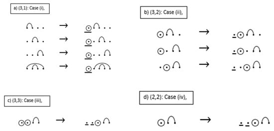
Figure 13.
Example of constructing the seven sequences with mutations and wobble base pairs.
The outline of the proof of Proposition 1 is illustrated by the cases given in the example below. For the given RNA sequences: Case (i) insert one base-point mutation to the leftmost position of the sequence; Case (ii) insert one unpaired base point (base point without a mutation) to the leftmost position of the sequence; Case (iii) delete one base-point mutation from the sequence, starting with the leftmost base-point mutation, substitute the deleted mutation with an unpaired base point at this position in the sequence, then insert an additional unpaired base point at the very beginning of the sequence; Case (iv) insert two unpaired base points to the leftmost position of the sequence. In addition, Proposition 1 and Theorem 4 have the same recurrence relations; thus, the proof of Proposition 1 is similar to the proof for Theorem 4. The proof for Theorem 4 is given after the example.
Thus, the lower triangular RNA array is interpreted as the number of RNA secondary structures with base-point mutations that contain wobble base pairs. Recall that wobble base pairs represent all entries of except for the entries of the leftmost column. Since the combinatorial arguments in the proof for Proposition 1 are similar to the combinatorial arguments in the proof of Theorem 4, we omit a formal proof for Proposition 1.
Let where counts RNA structures of length that have mutations and contain wobble base pairs. Let denote the set of RNA secondary structures of length with base-point mutations, where of the RNA sequences contain wobble base pairs. Before proving Theorem 4, as given below, we give the example = 20 which is illustrated in Figure 14, which has secondary structures with lengths of five and one base-point mutation. Of the twenty RNA sequences, seven sequences contain wobble base pairs and thirteen sequences do not contain wobble base pairs.
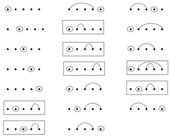
Figure 14.
Twenty RNA secondary structures with lengths of five and one base-point mutation, of which seven sequences contain wobble base pairs and thirteen sequences do not contain wobble base pairs.
Proposition 1, given above, confirms that ω is the entry of that counts the number of RNA secondary structures with mutations that contain wobble base pairs. The entry of w is associated with the entry of . We now give a combinatorial interpretation of in terms of RNA mutations with wobble pairs and non-wobble pairs.
Theorem 4.
Given the initial condition and the condition
, then for
and
,
satisfies the following recurrence relations
- (a)
- (b)
where (a) is defined for the leftmost column of
, (b) is defined for the other columns of
, and
counts RNA secondary structures of length
with
base point mutations where
of the structures contain wobble base pairs.
Proof.
Condition = 1 follows the definition of the restrictions placed on base-point mutations and wobble base pairs, and the way the entries are formed of . By convention, there is only one possibility for the condition . Suppose we have an RNA sequence of length with base-point mutations where of the sequences contain wobble pairs. Then, to form a new sequence of length with base-point mutations where of the structures contain wobble base pairs, we consider the following cases to prove recursion (b).
Case (i): If the given sequence has length with base-point mutations and of the sequences contain wobble pairs, where then there is one choice: to insert one base-point mutation to the leftmost position of the sequence with base-point mutations where of the sequences contain wobble pairs. In this case, all sequences whose leftmost point is a base-point mutation where ω of the sequences contain wobble pairs are counted by .
Case (ii): If the given sequence has length with base-point mutations and of the sequences contain wobble pairs, where then there is one choice: to insert one unpaired base point (base point without a mutation) to the leftmost position of the sequence with k base-point mutations where of the sequences contain wobble pairs. In this case, all sequences whose leftmost point is an unpaired base point where of the sequences contain wobble pairs are counted by .
Case (iii): If the given sequence has length with base-point mutations and of the sequences contain wobble pairs, where then there is one choice: to delete one base-point mutation from the sequence, starting with the leftmost base-point mutation. We substitute the deleted mutation with an unpaired base point at this position in the sequence. Then, we insert an additional unpaired base point at the very beginning of the sequence. We form an arc between the two new base points if they are not successive, and if they are successive, we do not form an arc. Note that from the construction of the sequence, no base-point mutations occur under an arc. In this case, all sequences with a substitution of a base-point mutation where of the sequences contain wobble pairs are counted by .
Case (iv): If the given sequence has a length of and base-point mutations and of the sequences contain wobble pairs, where then there is one choice: to insert two unpaired base points to the leftmost position of the sequence with k base-point mutations. In this case, all sequences whose two leftmost successive points are unpaired base points (base points without a mutation) where ω of the sequences contain wobble pairs are counted by .
Note that in Case (iii) there is an over count and Case (iv) accounts for an over count. This over count occurs in Case (iii) because we are deleting a base-point mutation and this produces, in some cases, the same structure as in Case (ii). Therefore, all sequences are removed from the count by Combining all of the cases accounts for all possible ways of forming where Applying the addition principle concludes that the recurrence relation (b) is proved. By similar reasoning we can prove part (a). □
This provides an elegant connection between RNA array I and RNA array II by the equation
where counts the RNA secondary structures of length with mutations given by [25]. Thus, as a consequence of and counts the number of RNA structures that contain non-wobble base pairs.
5.2. Bijection between Modified Walks and
Recall that are the lattice walks identified by Definition 4(b). In this subsection, we present modified unit-step lattice walks. Modified lattice walks consist of lattice walks with three different kinds of north steps denoted by N, , and , and two different kinds of south steps denoted by S and . These steps are subsequently described in the proof of Theorem 5. Since counts RNA secondary structures with base-point mutations where of the sequences contain wobble pairs and modified unit-step lattice walks, there exists an explicit bijection between these sets of combinatorial objects. See Figure 15 below for an example of the bijection. We now state and prove the following theorem.
Theorem 5.
There exists an explicit bijection between the set of modified unit-step lattice walks of length
ending at height
with consecutive north and south steps and the set of RNA secondary structures of length
with
base-point mutations where
of the sequences contain wobble pairs.
Proof.
To establish the required correspondence, let be an arbitrary secondary structure of length with base-point mutations where of the sequences contain wobble pairs. We write in its linear form as a sequence of bases, denoted by integers, increasing in order from left to right along a horizontal axis with n bases where the base-point mutations are denoted by ⊙. Arcs are drawn between two paired bases, allowing consecutive and non-consecutive bases to be paired. The arcs joining consecutive bases are wobble pairs.
Now, we will form a modified unit-step lattice walk as follows. Consider each ⊙ (i.e., base-point mutation) as an unpaired N (north) step, denoted by of the modified unit-step lattice walk. If a base is unpaired, label the base as an E (east) step. If an arc links non-consecutive integers and with , then label the th pairing members as non-consecutive (N, S) steps (non-wobble pairs). If an arc links consecutive integers and with , then label the th pairing members as consecutive (, ) steps (wobble pairs). Using the definition of , we confirm that the modified unit-step NSE** walks do not have consecutive south and north steps of any type of height and no two arcs intersect. Thus, there are no lattice walks with SN, N, S, or steps. However, S steps are allowed for lattice walks ending at height . To form a modified unit-step walk, we now have the following mappings: steps maps to N steps, (N, S) maps to unconsecutive N and S steps to form unconsecutive NS base pairs, (, ) maps to consecutive and steps to form consecutive steps, and E steps map to E steps. Note that (, ) and (N, S) steps will have the same number of and and N and S steps, respectively. The number of base-point mutations correspond to the height of modified unit-step lattice walks. From , we can obtain from the th entry of . The correspondence is constructed and reversible. Thus, the correspondence is one-to-one, and the theorem is proved. □
See Figure 7 for an example of a lattice walk ending at height . As an example of the bijection of a lattice walk ending at height (Theorem 5), consider one of the sequences of in Figure 15a below, where = w(11, 4) = 2307 is an entry of . Let be one secondary structure of length 12 with three base-point mutations. Of the structures, 2307 contain wobble base pairs. Applying the mapping, the integers are assigned as follows: 1, 2 , 3 , 4 N, 5 , 6 , 7 S, 8 E, 9 N, 10 , 11 , 12 S. We can then apply the rules of the correspondence to obtain one of the possible modified unit-step lattice walks with a length of 12, a height of three, and consecutive north and south steps given by Figure 15b.
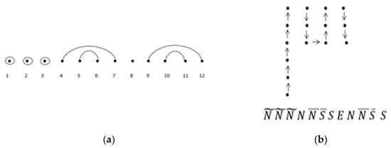
Figure 15.
(a) One representation of ; (b) corresponding modified unit-step NSE** lattice walk with a length of 12, a height of three, and consecutive north and south steps.
6. Concluding Remarks
RNA combinatorics is one of the primary mathematical tools used for RNA secondary structure prediction and analysis. The connection between RNA secondary structures and discrete mathematical biology (a subfield of enumerative combinatorics) is conveyed in this paper by manipulating generating functions, solving recurrence relations, analyzing RNA arrays as combinatorial matrices, and providing explicit bijections. We presented new explicit bijections involving certain subclasses of linear trees, lattice walks, and RNA secondary structures. We gave a generalized interpretation of , by taking -copies of , denoted by , and proved that the entries of the array count the number of -colored NSE* lattice walks. We combinatorically interpreted in terms of RNA base-point mutations and wobble base pairs. Since the entries of counted lattice walks as well as RNA secondary structures with base-point mutations where of the structures contain wobble base pairs, we established a new explicit bijection between these two combinatorial structures. These bijections provide combinatorial structural information that may provide insight into future biological applications of folding and modeling new RNA secondary structures. No RNA secondary structure prediction or folding was performed in this paper. See Evans [4] for applications and predictions of optimal RNA secondary folds of microRNAs related to tumor growth and cancer.
Future work in this field may include finding new bijections between RNA secondary structures, specifically structures that contain wobble base pairs, and modeling these structures to find new optimal viral RNAs. Finding bijections between and other combinatorial objects and modeling for some where are of interest for future work as well.
Author Contributions
Conceptualization, J.R.E.; methodology, J.R.E.; writing—original draft preparation, J.R.E.; writing—review and editing, A.N.; visualization, J.R.E.; supervision, A.N. All authors have read and agreed to the published version of the manuscript.
Funding
This research received no external funding.
Institutional Review Board Statement
Not applicable.
Informed Consent Statement
Not applicable.
Acknowledgments
The authors would like to thank Abdollah Dehzangi, Jonathan Farley, James Wachira, and Sarah Woodson for their support and comments on early versions of the paper. Special thanks to my husband, Eugene Evans, for his encouragement and discussions throughout the development of the paper. We also thank the referees for their useful comments.
Conflicts of Interest
The authors declare no conflict of interest.
References
- Heitsch, C.E. Combinatorics on Plane Trees, Motivated by RNA Secondary Structure Configurations, Preprint; University of Wisconsin: Madison, WI, USA, 2006. [Google Scholar]
- Reidys, C. Combinatorial Computational Biology of RNA: Pseudoknots and Neural Networks, 2011st ed.; Springer: New York, NY, USA, 2010. [Google Scholar]
- Waterman, M.S. Introduction to Computational Biology: Maps, Sequences and Genomes, 1st ed.; Chapman & Hall: London, UK, 1995. [Google Scholar]
- Evans, J. RNA Combinatorics and Secondary Structure Prediction with Applications to MicroRNA Structure Analysis. Ph.D. Thesis, Morgan State University, Baltimore, MD, USA, 2020. [Google Scholar]
- Chen, R. A new bijection between RNA secondary structures and plane trees and its consequences. Electron. J. Comb. 2019, 26, 48–63. [Google Scholar] [CrossRef]
- Barrera-Cruz, F.; Heitsch, C.; Poznanovic, S. On the structure of RNA branching Polytopes. SIAM J. Appl. Algebra Geom. 2018, 2, 444–461. [Google Scholar] [CrossRef]
- Cameron, N.T.; Sullivan, E. Peakless Motzkin paths with marked level steps at fixed height. Discrete Math. 2021, 344, 112154. [Google Scholar] [CrossRef]
- Deutsch, E.; Shapiro, L.W. A bijection between ordered trees and 2-Motzkin paths and its many consequences. Discrete Math. 2002, 256, 655–670. [Google Scholar] [CrossRef]
- Stein, P.R.; Waterman, M.S. On some new sequences generalizing the Catalan and Motzkin numbers. Discrete Math. 1979, 26, 261–272. [Google Scholar] [CrossRef]
- Willenbring, R. RNA secondary structure, permutations, and statistics. Discrete Appl. Math. 2009, 157, 1607–1614. [Google Scholar] [CrossRef]
- Lodish, H.; Berk, A.; Zipursky, S.L.; Krieger, M.; Scott, M.P.; Bretscher, A.; Ploegh, H.; Matsudaira, P. Molecular Cell Biology, 4th ed.; W. H. Freeman: New York, NY, USA, 2000. [Google Scholar]
- Darui, X.; Fenley, M.; Greenbaum, N.; Landon, T. The electrostatic characteristics of G·U wobble base pairs. Nucleic Acids Res. 2007, 35, 3836–3847. [Google Scholar]
- Clote, P.; Backofen, R. Computational Molecular Biology: An Introduction, 1st ed.; Wiley: New York, NY, USA, 2000. [Google Scholar]
- Hofacker, I.; Stadler, P. RNA Secondary Structures. In Encyclopedia of Molecular Cell Biology and MolecularMedicine; Meyers, R.A., Ed.; Wiley: Weinheim, Germany, 2006; pp. 581–603. [Google Scholar]
- Sankoff, D.; Zuker, M. RNA Structures and their prediction. Bull. Math. Biol. 1984, 46, 591–621. [Google Scholar]
- Parisien, M.; Major, F. Determining RNA three-dimensional structures using low-resolution data. J. Struct. Biol. 2012, 179, 252–260. [Google Scholar] [CrossRef]
- Sloane, N.J.A. The On-line Encyclopedia of Integer Sequences. 2001. Available online: http://www.research.att.com/njas/sequences/index.html (accessed on 1 December 2020).
- Nkwanta, A. Lattice paths and RNA secondary structures, DIMACS Series in Discrete Mathematics and Theoretical Computer Science. Am. Math. Soc. 1997, 34, 137–147. [Google Scholar]
- Nkwanta, A. Lattice paths, Riordan Matrices and RNA Numbers. Congr. Numer. 2008, 189, 205–216. [Google Scholar]
- Nkwanta, A. Lattice Paths, Generating Functions, and the Riordan Group. Ph.D. Thesis, Howard University, Washington, DC, USA, 1997. [Google Scholar]
- Cameron, N.T.; Nkwanta, A. Riordan matrices and lattice path enumeration. Not. Am. Math. Soc. 2023, 70, 231–242. [Google Scholar] [CrossRef]
- Luzón, A.; Merlini, D.; Morón, M.; Sprugnoli, R. Identities induced by Riordan arrays. Linear Algebra Appl. 2012, 436, 631–647. [Google Scholar] [CrossRef]
- Nkwanta, A. Riordan matrices and higher dimensional lattice walks. J. Stat. Plan. Infer. 2010, 140, 2321–2334. [Google Scholar] [CrossRef]
- Schmitt, W.R.; Waterman, M.S. Linear trees and RNA secondary structure. Discrete Appl. Math. 1994, 51, 317–323. [Google Scholar] [CrossRef]
- Rudra, S. Bijections among Linear Trees, Lattice Walks and RNA Base-Point Mutations. MA Thesis, Morgan State University, Baltimore, MD, USA, 2009. [Google Scholar]
- Heitsch, C.; Poznanovik, S. Combinatorial Insights into RNA Secondary Structure. In Discrete and Topological Models in Molecular Biology; Natural Computing, Series; Jonoska, N., Saito, M., Eds.; Springer: Berlin/Heidelberg, Germany, 2014; pp. 145–166. [Google Scholar]
- Howell, J.A.; Smith, T.F.; Waterman, M.S. Computation of generating functions for biological molecules. SIAM J. Appl. Math. 1980, 39, 119–133. [Google Scholar] [CrossRef]
- Waterman, M.S. Secondary Structures of single-stranded nucleic acids. In Studies in foundations and combina-torics, vol 1 of Advances in mathematics supplementary studies; Rota, G.C., Ed.; Academic Press: New York, NY, USA, 1978; pp. 167–212. [Google Scholar]
- Shapiro, L.W.; Getu, S.; Woan, W.J.; Woodson, L. The Riordan Group. Discrete Appl. Math. 1991, 34, 229–239. [Google Scholar] [CrossRef]
- Jean-Louis, C.; Nkwanta, A. Some algebraic structure of the Riordan group. Linear Algebra Appl. 2012, 438, 2018–2035. [Google Scholar] [CrossRef]
- Roman, S. An Introduction to Catalan Numbers, 1st ed.; Springer: Berlin/Heidelberg, Germany, 2015. [Google Scholar]
- Nkwanta, A.; Tefera, A. Curious Relations and Identities Involving the Catalan Generating Function and Numbers. J. Integer Seq. 2013, 16, 15. [Google Scholar]
- Loewe, L. Genetic mutation. Nat. Educ. 2008, 1, 113. [Google Scholar]
- Varani, G.; McLain, W.H. The G x U wobble base pair. EMBO Rep. 2000, 1, 18–23. [Google Scholar] [CrossRef] [PubMed]
Disclaimer/Publisher’s Note: The statements, opinions and data contained in all publications are solely those of the individual author(s) and contributor(s) and not of MDPI and/or the editor(s). MDPI and/or the editor(s) disclaim responsibility for any injury to people or property resulting from any ideas, methods, instructions or products referred to in the content. |
© 2023 by the authors. Licensee MDPI, Basel, Switzerland. This article is an open access article distributed under the terms and conditions of the Creative Commons Attribution (CC BY) license (https://creativecommons.org/licenses/by/4.0/).