Computational Optimized Monitoring Methodology to Avoid Crowd Crush Accidents with Scattered Data

Abstract

Recently, a crowd crush accident occurred in Seoul. Mathematics and data science can contribute to understanding this incident and to avoiding future accidents. In this paper, I suggest an optimized monitoring methodology to avoid crowd crush accidents with scattered data by searching the global minimum of the minimax data or minsum data. These scattered data are the position data of cell phones with time t. Mathematically, I find an exact solution of the optimized monitoring region with the suggested methodology by using the minimal constraints. The methodology is verified and validated along with the efficiency.

1. Introduction

Recently, at Itaewon in South Korea, a crowd crush accident occurred on 29 October 2022. This is a kind of crowing safety problem. Mathematics is contributed to analyze the data and to avoid the crowd crush accidents. In this paper, I suggest a mathematical methodology to help avoid these accidents. In real time, one can gather the position data of cell phones or head count data through CCTV. Monitoring centers have dependent variables—the longitude and latitude—and an independent variable—time t. These data are from the signals of satellites. Several local governments, agencies and organizations can gather crowd Geographic Information Systems (crowdGIS) data for public safety.

I suggest a real-time-dependent model using these data. With the longitude data and latitude data, the model is a two-dimensional space problem. If one adds the elevation data, then the model becomes a three-dimensional space problem. In the relative work, I extend this to N-dimensions in the optimization problem using the Kim method [1]. In this two-dimensional monitoring model, the measurement of optimization of these data has the key role in the performance of the methodology to monitor the risk of crowd crush accidents. Here, this paper focuses on the two-dimensional space problem. In the measurement of optimization, I describe either the minimax problem or minsum problem [2]. Here, the focus is on the minimax problem. The constrained optimization problem is then formulated as an unconstrained minimax problem of finding ${\mathbf{C}}^{*}$ such that

$$\begin{array}{c}\hfill J_{\infty }\left({\mathbf{C}}^{*}\right)=\underset{\mathbf{C}\in {\mathbb{R}}^2}{min}{J}_{\infty }\left(\mathbf{C}\right).\end{array}$$

(1)

In big data, one can extend the suggested problems with artificial intelligence, machine learning or deep learning. This is future research work.

The organization of the paper is as follows. Section 1 presents the introduction, background, problem statement and research contribution. The algorithm and the optimization methodology to solve the problem are described in Section 2 where I prove that the algorithm finds an exact minimax solution. The optimization methodology is verified. Then, in Section 3, the numerical results are presented, and the methodology is validated. The conclusions are given in Section 4.

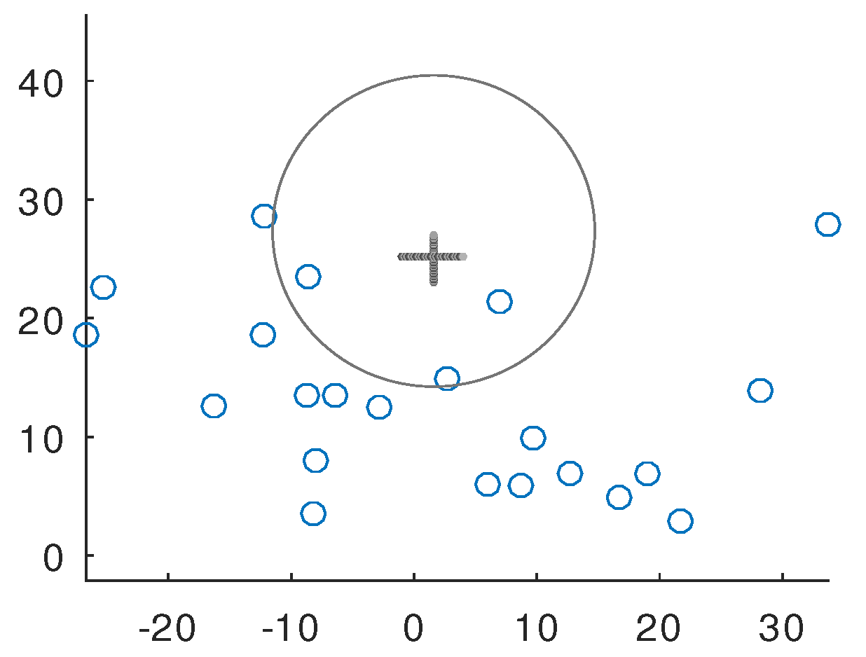
We need to denote the position ${\mathbf{P}}_i(x_i\left(t\right),y_i\left(t\right)),i=1,\cdots ,n\left(t\right)$ as the position of the cellphone in two-dimensional with the independent variable time t. First, we fix the time t for convenience and later, we extend to continuous models with time t. After we set the problem, to find the solution, we need the following constraint: Two fixed points, ${\mathbf{F}}_1$ and ${\mathbf{F}}_2$, are needed to begin the problem with the time t.

See Figure 1 for the suggested problem setting in the two-dimensional case. Here, the closeness of a circle to a set of points is given by the weighted maximum distance from the circle to the points. Denote, by $\mathbf{C}$, the center of a circle that passes through the two points ${\mathbf{F}}_1$ and ${\mathbf{F}}_2$, and, by $D_w\left(\mathbf{C}\right)$, the n-dimensional vector

$$D_w\left(\mathbf{C}\right)=\left(w_1{d}_1\left(\mathbf{C}\right),\cdots ,w_n{d}_n\left(\mathbf{C}\right)\right),$$

where $d_j\left(\mathbf{C}\right)=|{\mathbf{P}}_j-\mathbf{C}|-|{\mathbf{F}}_1-\mathbf{C}|,$ and the weight $w_j\in (0,1),$ $j=1,\cdots ,n.$

Set the objective function $J_p\left(\mathbf{C}\right)={\parallel D_w\left(\mathbf{C}\right)\parallel }_p$, where ${\parallel ·\parallel }_p$ denotes the ${\ell }^p$-norm for $1\le p\le \infty .$

A class of similar problems to (1) has a long history of development in operation research. This goes back to Pierre de Fermat who considered the case of $d_j\left(\mathbf{C}\right)=|{\mathbf{P}}_j-\mathbf{C}|$, $n=3$ and $p=1$ with equal weights whose solution is called the Fermat point. Consider the case of $d_j\left(\mathbf{C}\right)=|{\mathbf{P}}_j-\mathbf{C}|$, for a general n and $p=1$ with equal weights. Then, the problem is to find the geometric median of the set of points ${\mathbf{P}}_j,j=1,\cdots ,n,$ which is a standard problem in facility location to minimize the cost of transportation.

The minimizer ${\mathbf{C}}^{*}$ of $J_1\left(\mathbf{C}\right)$ is known as the Fermat–Weber [3] point or 1-median. The Fermat–Weber problem has drawn attention from mathematicians and facility location scientists and engineers; see, for instance [4,5,6,7,8,9,10,11,12,13,14,15,16], and the references therein. For the Euclidean metric $d(x,y)=\sqrt{{(x_1-y_1)}^2+{(x_2-y_2)}^2}$ only, see the references [8,9,10,11,12,14,15,16,17] and for the rectilinear (Manhattan) metric $d(x,y)=|x_1-y_1|+|x_2-y_2|$ and Euclidean metric, see the references [6,13]. For a survey paper on the Fermat–Weber problem, see Wesolowsky [18,19,20,21].

The case of $d_j\left(\mathbf{C}\right)=|{\mathbf{F}}_j-\mathbf{C}|-|{\mathbf{F}}_1-\mathbf{C}|,$ with equal weights without the constraint on the circle passing through any point was covered by Drezner [17] for $p=1,2,$ and ∞, and the case with equal and unequal weights was addressed by Brimberg et al. [22] for $p=\infty .$ Nonlinear minimax problems with successive approximation methods for finding a stationary point were also studied by Demjanov [23].

The suggested optimized optimization method (Kim method) in a two-dimensional case can be applied to the detection of a circle on the image [24]. The sphere-detection method (the Kim method in three-dimensions) can be applied to a three-dimensional image with depth.

This method is effective for big-data optimization problems of machine-learning models and algorithms [1,25]. The comparison study is shown in an N-dimensional research paper [1]. In a general N-dimensional model, the Kim method was verified and validated [1].

2. Optimization Methodology

The minimax crowd crush location optimization models are set up mathematically in this section. Let the cell phone location be ${\mathbf{P}}_j(x_j,y_j),j=1,\cdots ,n,$ with time t.

We suppose that two additional points ${\mathbf{F}}_1$ and ${\mathbf{F}}_2$ are given, which are distinct from ${\mathbf{P}}_i(x_i,y_i),i=1,\cdots ,l.$ Likewise, we set ${\mathbf{F}}_1$ and ${\mathbf{F}}_2$.

As described in the beginning of the section, this paper is restricted to the optimization model of finding a circle that passes through two given points. I propose a systematic approach to resolve this minimax model, thereby, obtaining an exact solution algorithm that is fast. The organization of the paper is as follows. The models are described in Section 2. I prove that the model methodology searches for an exact minimax solution. Then, in Section 3, the numerical results are presented. The conclusions are given in Section 4.

Since the circles are constrained to pass ${\mathbf{F}}_1$ and ${\mathbf{F}}_2$, the centers should lie on the straight line which bisects the line segment $\overline{{\mathbf{F}}_1{\mathbf{F}}_2}$ perpendicularly. To simplify the problem let us translate and rotate ${\mathbf{F}}_1$, ${\mathbf{F}}_2$ and ${\mathbf{P}}_i,i=1,\cdots ,l$ so that the locations of ${\mathbf{F}}_1$ and ${\mathbf{F}}_2$ are $(a,0)$ and $(-a,0)$ where $2a$ is the distance between ${\mathbf{F}}_1$ and ${\mathbf{F}}_2$. Furthermore, denote the coordinate of ${\mathbf{P}}_i$ by $(x_i,y_i),i=1,\cdots ,l$. Since the center of the circle lies on the y-axis, Problem (1) is then reduced to a one-dimensional problem. Denoting by $(0,u)$ the coordinate of $\mathbf{C}$, the radius of the circle, which passes through ${\mathbf{F}}_1$ and ${\mathbf{F}}_2$ is $\sqrt{u^2+a^2}$.

For $i=1,\cdots ,l,$ let ${\psi }_j\left(u\right)$ denote the weighted distance ${\varphi }_i\left(u\right)=\left|{\psi }_i\left(u\right)\right|$, where

$${\psi }_i\left(u\right)=w_i{d}_i\left(\mathbf{C}\right),d_i\left(\mathbf{C}\right)=\sqrt{{x_i}^2+{(u-y_i)}^2}-\sqrt{u^2+a^2}.$$

Since $D_w\left(\mathbf{C}\right)=\left({\psi }_1\left(u\right),\cdots ,{\psi }_l\left(u\right)\right),$ Problem (1) can be rewritten as finding $u^{*}\in \mathbb{R}$ such that

$$\begin{array}{c}\hfill \varphi \left(u^{*}\right)=\underset{u}{min}\varphi \left(u\right)\mathrm{where}\varphi \left(u\right):=\underset{i}{max}{\varphi }_i\left(u\right)=i_{\infty }\left(\mathbf{C}\right).\end{array}$$

(2)

Lemma 1.

Suppose that there does not exist a circle that passes through ${\mathbf{F}}_1$,${\mathbf{F}}_2$ and the data points ${\mathbf{P}}_i,i=1,\cdots ,l$. A local optimum to the minimax problem is then taken at the intersection point of the graphs of $y={\varphi }_{k_1}\left(u\right)$ and $y={\varphi }_{k_2}\left(u\right)$ for some $k_1$ and $k_2$. In the general $N—$dimensional case, see the reference [1].

Proof. 

Assume that the function $\varphi \left(u\right)$ has a local minimum at a point $u^{\prime }$, which is not an intersection point of any two graphs of $y={\varphi }_{k_1}\left(u\right)$ and $y={\varphi }_{k_2}\left(u\right)$ for any $k_1$ and $k_2$. Since the graph of $y=\varphi \left(u\right)$ is a finite number of piecewise smooth curves, there should exist some i and a sufficiently small positive $ϵ$ such that $\varphi \left(u\right)={\varphi }_j\left(u\right)$ on $(u^{\prime }-ϵ,u^{\prime }+ϵ)$ where $u^{\prime }$ is a critical point of $\varphi ,$ and thus it is a critical point of ${\varphi }_i$ thereon.

Such critical points should be either the zeros of the first derivative of ${\psi }_i\left(u\right)$ or the zero of ${\varphi }_i\left(u\right)$. Thus, the exact critical point $t^{\prime }$ of the function ${\varphi }_i\left(u\right)$ should be either $u_{\pm }=\frac{a{y}_j}{a\pm x_j},$ or $u_0=\frac{x_j^2+y_j^2-a^2}{2y_j},$ which are zeros of ${\psi }_i^{\prime }\left(u\right)=w_j(\frac{u-y_i}{\sqrt{x_i^2+{(u-y_i)}^2}}-\frac{u}{\sqrt{u^2+a^2}}),$ or ${\varphi }_i\left(u\right)$, respectively. In order to derive a contradiction from the existence of such critical points, notice that the second derivative of ${\psi }_i\left(u\right)$ is given as follows:

$$\begin{array}{ccc}\hfill {\psi }_j^{″}\left(u\right)& =& w_i(\frac{x_i^2}{{(x_i^2+{(u-y_i)}^2)}^{3/2}}-\frac{a^2}{{(u^2+a^2)}^{3/2}}).\hfill \end{array}$$

I treat the two cases separately.

(i)

First, let us consider the points $u^{\prime }=u_{\pm }$. Observe that

$${\psi }_i\left(u_{\pm }\right){\psi }_j^{″}\left(u_{\pm }\right)=-\frac{w_j^2\left(\right|a|-|x_i{\left|\right)}^2{(a\pm x_i)}^2}{|a{x}_i|}<0.$$

This means that if ${\psi }_i\left(u_{\pm }\right)$ is greater (or less) than zero, then ${\psi }_i^{″}\left(u_{\pm }\right)$ is less (or greater) than zero, and thus the function ${\psi }_i\left(u\right)$ has a local maximum (or local minimum) at $u_{\pm }$. Since ${\varphi }_i\left(u\right)=\left|{\psi }_i\left(u\right)\right|$, it follows that the function ${\varphi }_i\left(u\right)$ has a local maximum at $u_{\pm }$.

(ii)

Next, consider the point $u^{\prime }=u_0.$ Since the function $\varphi \left(u\right)$ has a local minimum at $u_0$ and $\varphi \left(u\right)={\varphi }_i\left(u\right)$ on $(u^{\prime }-ϵ,u^{\prime }+ϵ)$, it is trivial that $\varphi \left(u_0\right)={\varphi }_i\left(u_0\right)=0$.

Both cases (i) and (ii) lead to a contradiction to the assumption. Therefore, the local minimum of $\varphi \left(u\right)$ must be taken at a point $u^{\prime }$, which is an intersection point of two graphs of $y={\varphi }_{k_1}\left(u\right)$ and $y={\varphi }_{k_2}\left(u\right)$ for some $k_1$ and $k_2$. This completes the proof. □

The local minima of $y={\varphi }_{jk}\left(u\right)$ are taken at the intersection points of $y={\varphi }_j\left(u\right)$ and $y={\varphi }_k\left(u\right)$.

Theorem 2.

Let $t_{j,k}$’s be all the intersection points of the graphs of $y={\varphi }_j\left(u\right)$ and $y={\varphi }_k\left(u\right)$ for all $j,k=1,\cdots ,n.$ Let $u^{*}$ be such that

$$\varphi \left(u^{*}\right)=\underset{j,k}{min}\varphi \left(u_{j,k}\right).$$

If $\varphi \left(u^{*}\right)\le {max}_j{w}_j\left|y_j\right|$, then $\varphi \left(u^{*}\right)$ is a global minimum for Problem (2); otherwise, Problem (2) does not have a global minimum solution. In the general $N—$dimensional case, see the reference [1].

Proof. 

Let us begin with finding the candidates of global minimum of $\varphi \left(t\right)$ using the above Lemma 1. Since the equation ${\varphi }_j\left(u\right)={\varphi }_k\left(u\right)$ is equivalent to the equation ${\varphi }_j^2\left(u\right)={\varphi }_k^2\left(u\right)$, one can find the intersection points of ${\varphi }_j$ and ${\varphi }_k$ by solving

$$\begin{array}{ccc}\hfill 0& =& {\varphi }_j^2\left(u\right)-{\varphi }_k^2\left(u\right)\hfill \\ & =& \left(w_j\sqrt{x_j^2+{(u-y_j)}^2}-w_k\sqrt{x_k^2+{(u-y_k)}^2}-(w_j-w_k)\sqrt{u^2+a^2}\right)\hfill \\ & & \times \left(w_j\sqrt{x_j^2+{(u-y_j)}^2}+w_k\sqrt{x_k^2+{(u-y_k)}^2}-(w_j+w_k)\sqrt{u^2+a^2}\right)\hfill \\ & =:& I_1^w\left(u\right)\times I_2^w\left(u\right).\hfill \end{array}$$

(3)

Equation (3) is divided into $I_1^w\left(u\right)=0$ or $I_2^w\left(u\right)=0$.

To solve the equation $I_1^w\left(u\right)=0$, move the radical term $(w_j-w_k)\sqrt{u^2+a^2}$ to the right side of the equation and square both sides. Then, we find

$$\begin{array}{c}\hfill \begin{array}{cc}\hfill & (w_j^2+w_k^2)u^2-2(w_j^2{y}_j+w_k^2{y}_k)u+\{w_j^2(x_j^2+y_j^2)+w_k^2(x_k^2+x_k^2)\}\hfill \\ \hfill & -2w_j{w}_k\sqrt{x_j^2+{(u-y_j)}^2}\sqrt{x_k^2+{(u-y_k)}^2}\hfill \\ \hfill & ={(w_j-w_k)}^2(u^2+a^2).\hfill \end{array}\end{array}$$

To isolate the radical expression to the left side, move all the other terms to the right and square both sides of the equation again. Then, one gets the following cubic polynomial:

$$p_{jk}\left(t\right)=a_0{u}^3+a_1{u}^2+a_{2}u+a_3,$$

where

$$\begin{array}{cc}\hfill a_0& =8w_j{w}_k(w_j-w_k)(w_j{y}_j-w_k{y}_k),\hfill \\ \hfill a_1& =-4[\{w_j^2(x_j^2+y_j^2-a^2)+2w_j{w}_k{a}^2+w_k^2(x_k^2+y_k^2-a^2)\}{w}_j{w}_k\hfill \\ & +{(w_j^2{y}_j+w_k^2{y}_k)}^2-w_j^2{w}_k^2\{x_j^2+y_j^2+x_k^2+y_k^2+4y_j{y}_k\}],\hfill \\ \hfill a_2& =4\{w_j^2(x_j^2+y_j^2-a^2)+2w_j{w}_k{a}^2+w_k^2(x_k^2+y_k^2-a^2)\}(w_j^2{y}_j+w_k^2{y}_k)\hfill \\ & +8w_j^2{w}_k^2\{(x_j^2+y_j^2)y_k+(x_k^2+y_k^2)y_j\},\hfill \\ \hfill a_3& =-{\{w_j^2(x_j^2+y_j^2-a^2)+2a^2{w}_j{w}_k+w_k^2(x_k^2+y_k^2-a^2)\}}^2-4w_j^2{w}_k^2(x_j^2+y_j^2)(x_k^2+y_k^2).\hfill \end{array}$$

Similarly, solving the equation $I_2^w\left(u\right)=0$ is equivalent to solving the following cubic polynomial:

$$q_{jk}\left(u\right)=b_0{u}^3+b_1{u}^2+b_{2}u+b_3,$$

where

$$\begin{array}{cc}\hfill b_0& =8w_j{w}_k(w_j+w_k)(w_j{y}_j+w_k{y}_k),\hfill \\ \hfill b_1& =-4[\{w_j^2(x_j^2+y_j^2-a^2)-2w_j{w}_k{a}^2+w_k^2(x_k^2+y_k^2-a^2)\}{w}_j{w}_k\hfill \\ & -{(w_j^2{y}_j+w_k^2{y}_k)}^2+w_j^2{w}_k^2\{x_j^2+y_j^2+x_k^2+y_k^2+4y_j{y}_k\}],\hfill \\ \hfill b_2& =-4\{w_j^2(x_j^2+y_j^2-a^2)-2w_j{w}_k{a}^2+w_k^2(x_k^2+y_k^2-a^2)\}(w_j^2{y}_j+w_k^2{y}_k)\hfill \\ & +8w_j^2{w}_k^2\{(x_j^2+y_j^2)y_k+(x_k^2+y_k^2)y_j\},\hfill \\ \hfill b_3& ={\{w_j^2(x_j^2+y_j^2-a^2)-2w_j{w}_k{a}^2+w_k^2(x_k^2+y_k^2-a^2)\}}^2-4w_j^2{w}_k^2(x_j^2+y_j^2)(x_k^2+y_k^2).\hfill \end{array}$$

By using Cardano’s formula, one can find all the real roots of $p_{jk}\left(u\right)=0$ and $q_{jk}\left(u\right)=0$. In this way, one can find all the intersection points of $y={\varphi }_j\left(u\right)$ and $y={\varphi }_k\left(u\right)$ for $j,k=1,\cdots ,n.$ Then, by comparing the values of the function $\varphi \left(t\right)$ at these points, one can find the candidate of global minimum at $u^{*}$. As the function $\varphi \left(u\right)$ is defined on $\mathbb{R}$, the global minimum may not exist. However, using the expression

$${\varphi }_j\left(u\right)=\frac{w_j\left|x_j^2+y_j^2-a^2-2u{y}_j\right|}{\sqrt{x_j^2+{(u-y_j)}^2}+\sqrt{u^2+a^2}},$$

we have $\varphi \left(u\right)\to {max}_j{w}_j\left|y_j\right|$ as $u\to \pm \infty$. Thus, if $\varphi \left(u^{*}\right)\le {max}_j{w}_j\left|y_j\right|$, then $\varphi \left(u^{*}\right)$ is a global minimum. If $\varphi \left(u^{*}\right)>{max}_j{w}_j\left|y_j\right|$, then the function $\varphi \left(u\right)$ does not have global minimum. This completes the proof. □

Summarizing the above procedure in the proof of Theorem 2, we propose the following algorithm for solving the minimax problem (2):

Step1.

Compute the distance $2a$ between ${\mathbf{F}}_1$ and ${\mathbf{F}}_2$; choose the coordinates system such that ${\mathbf{F}}_1(a,0)$ and ${\mathbf{F}}_2(-a,0)$; by a rigid-motion transform to ${\mathbf{P}}_j$ associate all the coordinates $(x_j,y_j)$ for $j=1,\cdots ,n$;

Step2.

If ${\mathbf{F}}_1$, ${\mathbf{F}}_2$ and ${\mathbf{P}}_j,j=1,\cdots ,n$ are on one specific circle, then it is done.

Step3.

Find all the intersection points $u_{j,k}$’s of the graphs $y={\varphi }_j\left(u\right)$ and $y={\varphi }_k\left(u\right)$ for all $j,k;$

Step4.

For all such the intersection points $u_{j,k}$’s, evaluate ${\varphi }_i\left(u_{jk}\right)$ for all $i=1,\cdots ,n$; then compute $\varphi \left(u_{j,k}\right)={max}_i{\varphi }_i\left(u_{j,k}\right)$; and find the minimum $\varphi \left(u^{*}\right)={min}_{j,k}\varphi \left(u_{j,k}\right)$.

Step5.

If $\varphi \left(u^{*}\right)\le {max}_j{w}_j\left|y_j\right|$, then $\varphi \left(u^{*}\right)$ is the global minimum. If $\varphi \left(u^{*}\right)>{max}_j{w}_j\left|y_j\right|$, the global minimum of the function $\varphi \left(u\right)$ does not exist.

3. Numerical Results

I developed a minimax circle to monitor the crowd crush risk by using the position of a cell phone with time t. I show several test cases with 20 data of cell phone position including the weight $1.0$. See the

Table 1. ${\mathbf{F}}_{\mathbf{1}}$ = (5.00, 8.00) and ${\mathbf{F}}_{\mathbf{2}}$ = (−5.00, 2.00) are given with the equal weighted 20 points (Value is 1). The minimax value is $20.582$.

${\mathit{P}}_{\mathit{j}}$	${\mathit{x}}_{\mathit{j}}$	${\mathit{y}}_{\mathit{j}}$
$P_1$	2.700	4.900
$P_2$	−0.200	3.53
$P_3$	4.97	1.40
$P_4$	−2.30	8.63
$P_5$	8.70	13.9
$P_6$	−8.20	3.53
$P_7$	19.00	6.90
$P_8$	−12.3	8.63
$P_9$	33.7	27.9
$P_{10}$	−25.3	22.6
$P_{11}$	6.70	4.90
$P_{12}$	−6.20	3.53
$P_{13}$	2.7	1.92
$P_{14}$	−26.3	18.6
$P_{15}$	8.37	15.9
$P_{16}$	−8.62	23.5
$P_{17}$	9.97	9.90
$P_{18}$	−16.3	2.63
$P_{19}$	21.7	2.90
$P_{20}$	−15.3	9.83
Solution	−13.413	27.355

,

Table 2. ${\mathbf{F}}_{\mathbf{1}}$ = (6.00, 6.00) and ${\mathbf{F}}_{\mathbf{2}}$ = (−8.00, 8.00) are given with the equal weighted 20 points (Value is 1). The minimax value is $13.117$.

${\mathit{P}}_{\mathit{j}}$	${\mathit{x}}_{\mathit{j}}$	${\mathit{y}}_{\mathit{j}}$
$P_1$	2.700	14.900
$P_2$	−8.7200	13.50
$P_3$	6.97	21.40
$P_4$	−12.30	18.63
$P_5$	28.20	13.9
$P_6$	−8.20	3.53
$P_7$	19.0	6.90
$P_8$	−12.2	28.60
$P_9$	33.7	27.9
$P_{10}$	−25.3	22.6
$P_{11}$	16.7	4.90
$P_{12}$	−6.42	13.50
$P_{13}$	12.7	6.92
$P_{14}$	−26.7	18.6
$P_{15}$	8.70	5.90
$P_{16}$	−8.62	23.5
$P_{17}$	9.70	9.90
$P_{18}$	−16.3	12.6
$P_{19}$	21.7	2.90
$P_{20}$	−2.83	12.5
Solution	1.5994	25.196

and

Table 3. ${\mathbf{F}}_{\mathbf{1}}$ = (25.00, 18.00) and ${\mathbf{F}}_{\mathbf{2}}$ = (−25.00, 12.00) are given with the equal weighted 20 points (Value is 1). The minimax value is $15.5322$.

${\mathit{P}}_{\mathit{j}}$	${\mathit{x}}_{\mathit{j}}$	${\mathit{y}}_{\mathit{j}}$
$P_j$	$x_j$	$y_j$
$P_1$	−16.20	23.50
$P_2$	12.700	21.90
$P_3$	−26.30	28.60
$P_4$	18.40	15.90
$P_5$	−8.62	23.50
$P_6$	20.00	9.90
$P_7$	−16.30	2.63
$P_8$	21.70	22.90
$P_9$	−15.30	9.83
$P_{10}$	12.70	4.90
$P_{11}$	−0.20	3.53
$P_{12}$	15.00	21.40
$P_{13}$	−2.30	28.60
$P_{14}$	8.70	13.90
$P_{15}$	−8.20	23.50
$P_{16}$	19.00	6.90
$P_{17}$	−12.30	28.60
$P_{18}$	33.70	27.90
$P_{19}$	−25.3	22.60
$P_{20}$	26.7	4.90
Solution	−0.32476	17.706

. The Table shows the detailed input data with the weights (the weights are 1). ${\mathbf{C}}^{*}$ is the numerical solution from the exact solution procedure of the suggested models. I tested many times for various random input data and the results are satisfactory. The computation is executed using the fortran compiler in a window system with the architecture Intel Pentium CPU 4405U of 2.10 GHz. See Figure 2 for the validation. The verification was proved in Section 2. 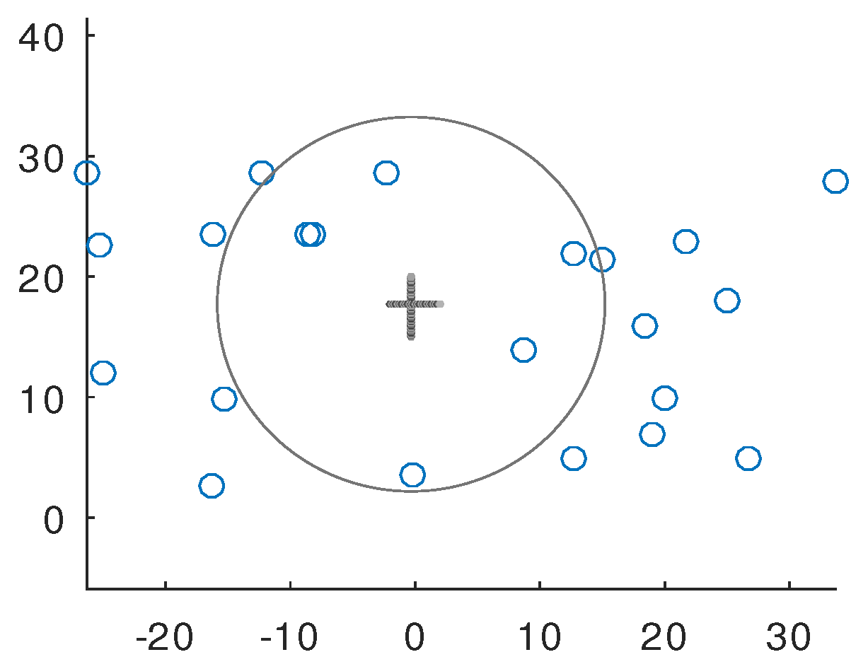See Figure 3, Figure 4 and Figure 5 for the fixed single time t. 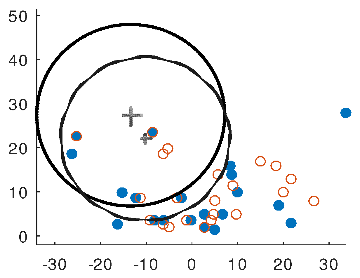Figure 6 and Figure 7 were shown for the multiperiod.

Generally, in N-dimensional, I performed the comparison study with the suggested methodology and other methodology of the data [1,26]. See the

Table 4. AUC values for a dataset with a sample size of 200 with other methodologies [1,26].

$\mathit{K}\mathit{I}\mathit{M}$	$\mathit{D}\mathit{T}$	$\mathit{k}-\mathit{N}\mathit{N}$	$\mathit{L}\mathit{o}\mathit{g}\mathit{R}$
$1.0000$	0.7941	0.7683	0.6328
$NB$	$C4.5$	$SVM$	$LC$
0.7126	0.7452	0.7448	0.6408

with a comparison study of several methodology with the random data set from [26]. AUC is the area under the curve. The method result of AUC (KIM) has $1.0000$ in Table 4 because the two distinct circles are not overlapped. DT is the decision tree method. $k-NN$ is the k-nearest neighbor method. $LogR$ is the logistic regression method. NB is the Naive Bayes method. C4.5 is a decision tree with divide-and-conquer. SVM is the support vector machine method. LC is the linear classifier method [26]. The methodology is to find the mathematical exact solution. I find the two distinct circle with centers and radii.

4. Conclusions

This paper proposed an optimized monitoring methodology to avoid crowd crush accidents with scattered data by searching the global minimum of the minimax data or minsum data with the independent variable time t. These scattered data are the position data of cell phones with time t. Mathematically, I found an exact solution of the optimized monitoring region with the suggested methodology using the Kim method [1].

This paper investigated the suggested minimax problem with the suggested optimization method (the Kim method). This problem was applied to analyze monitoring to avoid crowd crush accidents. Here, I also considered the general weighted case. The weighted value can be considered as the historical value of the risk of the crowd crush possibility. Furthermore, I obtained the exact solution of the minimizing circle to avoid the risk of crowd crush accidents by maximizing the distance between the circle through two fixed points and multiple points. By finding the local optima, one finds the global optimum.

After verifying and validating the exact solution of monitoring with the suggested monitoring problem, an efficient algorithm was proposed. The advantage of this methodology is to theoretically find the exact solution. Thus, one can save on computation time by using the exact formula to find the coefficients of the equations. This is the optimization method of 2D scattered cell phone position data. This contributes to the analysis of monitoring for crowd crush accidents.