Modeling a Spheroidal Particle Ensemble and Inversion by Generalized Runge–Kutta Regularizers from Limited Data

Abstract

Extracting information about the shape or size of non-spherical aerosol particles from limited optical radar data is a well-known inverse ill-posed problem. The purpose of the study is to figure out a robust and stable regularization method including an appropriate parameter choice rule to address the latter problem. First, we briefly review common regularization methods and investigate a new iterative family of generalized Runge–Kutta filter regularizers. Next, we model a spheroidal particle ensemble and test with it different regularization methods experimenting with artificial data pertaining to several atmospheric scenarios. We found that one method of the newly introduced generalized family combined with the L-curve method performs better compared to traditional methods.

1. Introduction

We denote with $\mathcal{L}(V,G)$ the set of linear bounded operators between the normed spaces V and G with the inner products ${\langle ·,·\rangle }_V$ and ${\langle ·,·\rangle }_G$, respectively, and $\mathcal{K}(V,G)=\{T\in \mathcal{L}(V,G\left)\right|T\mathrm{is}\mathrm{compact}\}$. Note that we often omit the space-subscripts in the inner products for brevity when there is no risk of confusion.

Compact linear operators $Tv=g$ are the extension of matrices in Hilbert spaces, in which one is able to generalize the spectral theorems. A special compact linear operator which models our problem in Atmospheric Physics, the spheroidal particle ensemble, and many other applications, arises from the Fredholm operator of the first kind. The Fredholm integral equation has the following general form:

$$Tv={\int }_a^{b}K(\lambda ,r)v\left(r\right)dr=g\left(\lambda \right),$$

(1)

where $K(\lambda ,r)$ is the kernel function. In Section 4, we show an example of such a function representing backscatter and extinction cross sections of aerosol particles. The Riemann–Lebesgue Lemma indicates the underlying reason for the ill-posedness of these integral equations. Consider the function sequence $v_n\left(r\right)=sin\left(2n\pi r\right)$. Then, for a Riemann-integrable function $K(s,t)$, it holds

$$\underset{n\to \infty }{lim}{\int }_0^{1}K(\lambda ,r)v_n\left(r\right)dr\to 0.$$

(2)

This result summarizes the smoothing phenomenon imposed by the Fredholm operator to any solution candidate.

The properties of the Singular Value Decomposition (SVD) of the operator are given by: Let $T\in \mathcal{K}(V,G)$ and let $T^{*}$ be the adjoint of T. There exist sequences $f_j\in V$, $h_j\in G$, and ${\mu }_j\in \mathbb{R}$ with $0<{\mu }_{j+1}\le {\mu }_j$ and $j\in \mathbb{N}$ such that the following statements hold:

1.

${lim}_{j\to \infty }{\mu }_j=0$.

2.

The sequences ${\left\{h_j\right\}}_{j\in \mathbb{N}}$ and ${\left\{f_j\right\}}_{j\in \mathbb{N}}$ form a complete orthonormal system of the spaces $\overline{\mathrm{im}\left(T\right)}$ and $\overline{ker{\left(T\right)}^{\perp }}$, respectively:

3.

$T{f}_j={\mu }_j{h}_j$ and $T^{*}{h}_j={\mu }_j{f}_j$ for all $j\in \mathbb{N}$.

4.

$Tv={\sum }_{j=1}^{\infty }{\mu }_j{\langle v,f_j\rangle }_V{h}_j$, and $T^{*}v={\sum }_{j=1}^{\infty }{\mu }_j{\langle v,h_j\rangle }_G{f}_j$ for all $v\in V$.

The triple ${({\mu }_j,f_j,h_j)}_{j\in \mathbb{N}}$ is called the singular system of the compact operator T. In particular, the sequences ${\left\{f_j\right\}}_{j\in \mathbb{N}}$ and ${\left\{h_j\right\}}_{j\in \mathbb{N}}$ are called the left and right singular functions, respectively, and the sequences ${\left\{{\mu }_j\right\}}_{j\in \mathbb{N}}$ are called the singular values of T.

Furthermore, the Picard condition states the following: Let $T:V\to G$ be a compact operator and ${({\mu }_j,f_j,h_j)}_{j\in \mathbb{N}}$ its singular system. An element $g\in \overline{\mathrm{im}\left(T\right)}$ is an element of $\mathrm{im}\left(T\right)$ exactly, when

$$\sum _{j=1}^{\infty }{\left(\frac{|\langle g,h_j\rangle |}{{\mu }_j}\right)}^2<\infty .$$

(3)

This condition exposes the decisive role of the convergence rate of the singular values; there only exists a solution if the terms $|\langle g,h_j\rangle |$ decay faster in competition to the singular values.

Regularization methods are very good candidates in order to gain some control over noisy and highly sensitive solutions and to solve inverse ill-posed problems efficiently. One family of methods, that can be used for regularization, is the one of Runge-Kutta integrators, commonly used for ordinary differential equations.

For linear operators, Rieder [1] proved that Runge–Kutta integrators applied to the asymptotic regularization and stopped by the discrepancy principle are regularization schemes where the Hölder-type source set $X_{\nu ,\rho }:=\{{\left(A^{*}A\right)}^{\nu }z:z\in N{\left(A\right)}^{\perp },\parallel z\parallel \le \rho \}$ is used. Recently, in Pornsawad et al. [2], a modified discrepancy principle was investigated for the implicit Euler method of the Runge–Kutta family. In Böckmann et al. [3] and Pornsawad et al. [4,5], the nonlinear operator case was investigated under Hölder-type and logarithmic source conditions. It was shown that convergence and optimal convergence rates can be achieved under certain assumptions. Similarly, in Zhao et al. [6], a wide class of spectral regularization methods under variational source conditions was shown to yield convergence rates under certain general assumptions, which are also satisfied by asymptotic regularization and Runge–Kutta integrators.

This paper is structured in the following manner: first, in Section 2, a brief review of regularization methods is given to build up a necessary background, also useful for the investigation of the spheroidal particle model later on. In Section 3, we propose a new generalized filter of the Runge–Kutta type and prove regularizing properties of such a filter. Readers, only interested in the application in Atmospheric Physics, may skip Section 2 and Section 3. Furthermore, Section 4 and Section 5 are dedicated to the modeling of a spheroidal particle ensemble and our numerical experiments with different atmospheric scenarios, respectively. The latter is done by means of gradual complexity moving from spherical- to non-spherical particle ensembles and retrieving particle distributions of one and two dimensions, respectively. This serves us in order to introduce a new method and demonstrate its efficiency for the problem of aerosol microphysics in the 1D case (Mie model), which most of the literature is occupied with, and then extend to the quasi-2D case we mostly focus on. Section 5 is also concerned with the reconstruction of shape-size distributions with modality up to 2. Section 6 summarizes the upsides and limitations.

2. Preliminaries: Brief Review of Regularization Theory

A well-posed problem has a unique solution which depends on the input data in a stable manner. A problem that violates any of the three properties of well-posedness (existence, uniqueness or stability) is called an ill-posed problem. The degree of ill-posedness is given by: Let $\mathcal{M}$ be a positive real number. Then, the problem (T, V, G)

1.

is mildly ill-posed if ${\mu }_j$ has a polynomial behaviour, i.e., ${\mu }_j=\mathcal{O}\left(j^{-\mathcal{M}}\right)$.

2.

is severely ill-posed if ${\mu }_j$ has an exponential behaviour, i.e., ${\mu }_j=\mathcal{O}\left(e^{-\mathcal{M}j}\right)$.

The ambiguity in the solution space is apparently undesired. It is possible to search for a unique solution by replacing the problem with

$$T^{*}Tv=T^{*}g⟺T^{*}(Tv-g)=0⟺Tv-g\in ker\left(T^{*}\right)=\mathrm{im}{\left(T\right)}^{\perp },$$

(4)

which turns out to be equivalent to a least-squares problem.

For $g\in \mathrm{im}\left(T\right)\oplus \mathrm{im}{\left(T\right)}^{\perp }$, the set of the solutions of the normal equation $T^{*}Tv=T^{*}g$ is non-empty, closed and convex. Moreover, there is a unique solution $v^{†}$ of minimal norm.

This property of the normal equation along with continuity of the norm allows the existence of a unique solution of minimal norm and strikes out uniqueness from Hadamard’s requirements [7]. We shall define this as a solution of $Tv=g$ in generalized terms.

The operator $T^{†}:\mathcal{D}\left(T^{†}\right)\to V$, with the domain $\mathcal{D}\left(T^{†}\right):=\mathrm{im}\left(T\right)\oplus \mathrm{im}{\left(T\right)}^{\perp }$, which assigns uniquely an element $v^{†}$ of minimal norm to any $g\in \mathcal{D}\left(T^{†}\right)$ is called a Moore–Penrose inverse or generalized inverse of $T\in \mathcal{L}(V,G)$. The element $v^{†}=T^{†}g$ is called the minimum-norm solution of $Tv=g$.

We are now able to answer by what means and under which circumstances we can invert the equation $Tv=g$.

Theorem 1.

Let $T\in \mathcal{L}(V,G)$; then, its generalized inverse $T^{†}$ has the following properties:

1. 

$v^{†}=T^{†}g$ is the unique solution of the normal equation $T^{*}Tv=T^{*}g$ in $ker{\left(T\right)}^{\perp }$, for every $g\in \mathcal{D}\left(T^{†}\right)$.

2. 

$T^{†}$ is linear.

3. 

$\mathrm{im}\left(T^{†}\right)=ker{\left(T\right)}^{\perp }$.

4. 

$T^{†}$ is continuous if and only if $\mathrm{im}\left(T\right)$ is closed. Then, $T^{†}$ is defined in the whole G.

5. 

If T is compact, then it is continuous if $\mathrm{im}\left(T\right)$ is finite.

The key to assure the well-posedness of our problem is $\mathrm{im}\left(T\right)=\overline{\mathrm{im}\left(T\right)}$. In fact, this allows for characterization of ill-posedness through the closedness of the range $\mathrm{im}\left(T\right)$. The ill-posedness by Nashed is defined as follows: The problem $(T,V,G)$ is called ill-posed if $\mathrm{im}\left(T\right)$ is not closed [8]. Otherwise, it is called well-posed.

2.1. Regularization with Spectral Filters

First, let us define regularization through a family of operators approximating the desired (generalized) inverse, see e.g., [9,10].

Definition 1

(Regularization Scheme). The family of linear bounded operators ${\left\{R_{\zeta }\right\}}_{\zeta >0}$ from G into V is called a regularization scheme or a regularizer for T if we have the following pointwise convergence:

$$\underset{\zeta \to 0}{lim}{R}_{\zeta }Tv=v,\mathrm{for}\mathrm{all}v\in V.$$

(5)

Let there be given noisy data with$g^{\delta }$,$\delta >0$, with$\parallel g^{\delta }-g\parallel <\delta$and let${\left\{R_{\zeta }\right\}}_{\zeta >0}$be a regularization scheme, where$\zeta =\zeta (\delta ,g^{\delta })>0$. If, for all$g\in \mathrm{im}\left(T\right)$and all$g^{\delta }\in G$with$\parallel g^{\delta }-g\parallel <\delta$we have

$$\underset{\delta \to 0}{lim}{R}_{\zeta }{g}^{\delta }=T^{†}g,$$

(6)

then the pair$(R_{\zeta },\zeta )$is called a regularization method for$Tv=g$. Furthermore,$\zeta$is called a priori parameter choice rule (PCR) if it only depends on$\delta$; otherwise, it is called a posteriori parameter choice rule.

Note that a PCR depending solely on $g^{\delta }$ is called a data-driven one and is often based on heuristics.

In case we have a unique solution $v^{†}=T^{†}g={\left(T^{*}T\right)}^{-1}{T}^{*}g$, we can see that the troubling part, regarding stability, is the operator $T^{*}T$. Moreover, recalling the singular system of T, ${({\mu }_j,f_j,h_j)}_{j\in \mathbb{N}}$, we have $T^{†}={\sum }_{j=1}^{\infty }{\mu }_j^{-1}\langle ·,h_j\rangle f_j\left(r\right)$ and therefore our filters need to target the singular values. This motivates the filter function $b(\zeta ,\mu )$ for the regularization scheme

$$R_{\zeta }{g}^{\delta }=\sum _{j=1}^{\infty }b(\zeta ,{\mu }_j){\mu }_j^{-1}\langle g^{\delta },h_j\rangle f_j\left(r\right).$$

(7)

An immediate question is what the properties of such a function are in order to constitute a regularization method.

Theorem 2

(Regularizing filters). Let T be an injective compact operator with singular system ${({\mu }_j,f_j,h_j)}_{j\in \mathbb{N}}$. If the function $b:(0,\infty ]\times (0,\parallel T\parallel ]\to \mathbb{R}$ satisfies the following conditions:

1. 

$b(\zeta ,\mu )$ is bounded for all $\zeta >0,\mu \in (0,\parallel T\parallel ]$ and ${lim}_{\zeta \to 0}b(\zeta ,\mu )=1$ for all $\mu \in (0,\parallel T\parallel ]$,

2. 

for all $\zeta >0$, there exists a positive constant $d\left(\zeta \right)$ such that all $\mu \in (0,\parallel T\parallel ]$ hold either of the following relations:

2.1. 

$\left|b\right(\zeta ,\mu \left)\right|\le d\left(\zeta \right)\mu$

2.2. 

$\left|b(\zeta ,\mu )\right|\le d\left(\zeta \right){\mu }^2$

then $R_{\zeta }$ is a regularization scheme defined as in (7), and $v^{(\delta ,\zeta )}=R_{\zeta }{g}^{\delta }$. Moreover, we have $\parallel R_{\zeta }\parallel \le \tau$ and the reconstruction error estimate

$$\parallel v^{(\delta ,\zeta )}{-v\parallel }^2\le {\parallel v\parallel }^2\underset{\mu \in (0,\parallel T\parallel ]}{sup}{|b(\zeta ,\mu )-1|}^2+{\delta }^2{\tau }^2,$$

(8)

where $\tau =d\left(\zeta \right)$ in case of (i) or $\tau =\sqrt{Cd\left(\zeta \right)}$ in case of (ii) with C denoting a bound on q. The function $b(\zeta ,\mu )$ is then called a regularizing filter.

A proof can be found, e.g., in [10]. Examples of filter functions will now be introduced amid the exposé of the methods we are going to use later in our simulations.

2.1.1. Truncated SVD

Here, we only show a discrete analog of SVD of practical interest: For any matrix $M\in {\mathbb{R}}^{m\times n}$, there exist orthogonal matrices $U\in {\mathbb{R}}^{m\times m}$ and $V\in {\mathbb{R}}^{n\times n}$ and a matrix $\Sigma =\mathrm{diag}({\sigma }_1,{\sigma }_2,\dots ,{\sigma }_r)\in {\mathbb{R}}^{m\times n}$ where $r=min\{m,n\}$ and ${\sigma }_1\ge {\sigma }_2\ge \cdots \ge {\sigma }_p>{\sigma }_{p+1}=\cdots ={\sigma }_r=0$, so that M is decomposed to

$$M=U\Sigma V^T=\sum _{i=1}^p{\sigma }_i{\upsilon }_i{\nu }_i^T,$$

(9)

where ${\upsilon }_i,{\nu }_i$ are the orthonormal columns of U and V, and they are called left and right singular vectors of M, respectively. The ${\sigma }_i$-s are called singular values of M, and the triple $({\sigma }_i,{\upsilon }_i,{\nu }_i)$ is called singular system of M. Tiny singular values (close to zero) are the ones responsible for a disproportionate increase in error induced high frequencies; the steeper the decay rate, the higher the degree of ill-posedness. Intuitively, this suggests keeping only the most significant singular values and discard the rest. A threshold $\zeta >0$ will be the cut-off (regularization) parameter below which no singular value makes it to the sum. We summarize this discussion to the introduction of the reqularizing filter b of what we call the Truncated SVD (TSVD):

$$b(\zeta ,\mu )=\left\{\begin{array}{cc}1,\hfill & \mu \ge \zeta \hfill \\ 0,\hfill & \mathrm{otherwise}\hfill \end{array}\right.$$

(10)

2.1.2. Tikhonov Regularization

TSVD is a straightforward regularization tool which aims to identify and cut out the most vulnerable part of the solution. However, doing so it wastes all the solution information associated with the disposed part. Furthermore, in cases where there is a lot of noise, the “ripping” nature of TSVD may result in an oversmoothed solution. Therefore, instead of cutting some part, we can alternatively give it a shift by a parameter ${\zeta }^2$$(\zeta >0)$ to counteract its spectral weakness. This correcting procedure, enabling the search of an optimal balance ($\zeta$) of the good against the troubling solution content, is attributed to A.N. Tikhonov [11]. The concept of Tikhonov Regularization (TR) is described by the filter function b:

$$b(\zeta ,\mu )=\frac{{\mu }^2}{{\mu }^2+{\zeta }^2}.$$

(11)

We introduced Tikhonov’s method from the point of view of the singular values following a possible flaw of the behavior of SVD. There are, nevertheless, a few ways to define this method basically through a minimization procedure, see e.g., [12].

2.1.3. Iterative Regularization Methods: Runge–Kutta Integrators

Let the following be an initial value problem:

$$\begin{array}{cc}\hfill \dot{v}& =H(v,t),t>0\hfill \\ \hfill v& \left(t_0\right)=v_0.\hfill \end{array}$$

(12)

Choosing a step size $0<h=t_j-t_{j-1}$, $j=1,2,\dots ,N$. We seek an approximation $v_j=v\left(t_j\right)$, given by the formula:

$$v_j=v_{j-1}+h\sum _{n=1}^k{z}_n{r}_n,$$

(13)

where

$$r_i=H\left(t+c_{i}h,v+h\sum _{s=1}^k{m}_{is}{r}_s\right),\mathrm{for}i=1,2,\dots ,k$$

(14)

is the i-th stage of the (generally implicit) Runge–Kutta method. Considering $m_{ij}$, $c_j$, $z_j$ as the matrix elements of $M^{k\times k}$, ${\mathbf{c}}^{k\times 1}$, and ${\mathbf{z}}^{k\times 1}$, respectively, the formalism is lightened by the mnemonic device

$\mathbf{c}$	M
	${\mathbf{z}}^{\mathbf{T}}$

called the Butcher’s tableau, developed in 1960 by J.C. Butcher [13]. In our case, we have $H\left(v\right)=-T^{*}Tv+T^{*}g$. This iterative filter method was first introduced in [1,14,15] and will be studied in more detail in the next Section.

2.2. Parameter Choice Rules

Regularization describes the way to reverse the noise effect and restore partly the “natural” regularity of the solution but does not prescribe the depth of its act inherently. The use of parameter choice rules is not an optional addition but necessary in order to make a regularization method successful, or in other words, to minimize regularization errors in some sense. Here, we present the most widely used PCRs in bibliography and those which we are using later in our application, highlighting their assets and drawbacks.

Among all the parameter choice rules, the discrepancy principle is the most facile both conceptually and computationally. It is based on the “reasonable” demand that the data should be approximated with a same-order accuracy as the actual (measurement) data error. The obvious dependence on distorted-data information ($g^{\delta }$) classifies this technique as an a posteriori PCR. This technique, Morozov’s discrepancy principle, is formalized as follows. Let $v^{(\zeta ,\delta )}$ be the regularized solution of $Tv=g$ produced by the regularization method $(R_{\zeta (\delta ,g^{\delta })},\zeta )$ and let $c>1$ be a constant. The regularization parameter ${\zeta }^{*}\le \zeta$ is determined such that

$$\parallel T{v}^{({\zeta }^{*},\delta )}-g^{\delta }\parallel \le c\delta <\parallel T{v}^{(\zeta ,\delta )}-g^{\delta }\parallel .$$

(15)

The constant c is often called the safety factor and allows a somewhat safer approach preventing possible oversmoothing.

Despite the unique ease of the discrepancy principle, insufficient knowledge on the error level often strikes it out as an option. This is the basic motivation behind the development of PCRs solely based on the available data. The idea behind the L-curve method lies within the plot of the regularity term against the residual error, first suggested by [16]. The L-curve criterion is summarized as follows: Let $(\tilde{J},\tilde{I})=\left(log\parallel T{v}^{(\zeta ,\delta )}-g^{\delta }\parallel ,log\parallel Q{v}^{(\zeta ,\delta )}\parallel \right)$ be the points constituting the L-curve. The regularization parameter is determined by maximizing its curvature function $\omega \left(\zeta \right)$ [17,18]

$$\omega \left(\zeta \right)=\frac{{\tilde{J}}^{\prime }{\tilde{I}}^{\prime \prime }-{\tilde{J}}^{\prime \prime }{\tilde{I}}^{\prime }}{{[{({\tilde{J}}^{\prime })}^2+{({\tilde{I}}^{\prime })}^2]}^{3/2}}.$$

For our purposes, we will use the L-curve criterion combined either with the Tikhonov method or with our iterative regularization. The L-curve method solves heuristically the bargain between the competing error terms (approximation and data error), but there are some obstacles to oversee. The resulting plots for a noisy right-hand side ($g^{\delta }$) are neither always “L-shaped” (missing the vertical or horizontal part, or having “local” corners, or being arbitrary shaped) nor a curve, in cases where the regularization parameter is discrete (e.g., the cut-off level of TSVD), in which case the inversion is assisted by interpolation. All the latter scenarios might result in an occasional failure of the method. We note that in this work, for the combination of an iterative regularization (Runge-Kutta) with the L-curve, where the number of iterations is the regularization parameter, we “fill in” the gaps of the discrete L-curve with cubic spline interpolation.

Finally, cross validation [19] is a well-known learning algorithm from statistics, offering another purely-data-driven regularization method. All previous PCRs do not take into account how good a prediction would be with data that the procedure has not been “trained” to deal with. The first step of this approach includes splitting the data in sets of “training” and “test”. Then, the model equation “learns” by being inverted for the data in the training set and subsequently uses this knowledge $v_{-}^{(\zeta ,\delta )}$ (“-” expresses the missing data) to reproduce the data from the test set with forward calculations ($R_{\zeta }{v}_{-}^{(\zeta ,\delta )}$). Finally, the mean error from the predictions is used to evaluate the prediction.

In this work, we will use the “leave-one-out” partition, which removes only a single point, trains with the rest and goes back to predict the missing one. This is repeated for every data point, and the regularization parameter is chosen so that the mean prediction error is minimized. In our application, we use TR with GCV. The regularization parameter is determined by minimizing the so-called GCV function $\omega \left(\zeta \right)$

$$\omega \left(\zeta \right)=\frac{\parallel T{v}^{(\zeta ,\delta )}-g^{\delta }{\parallel }^2}{{\left(m-{\sum }_{i=1}^{n}b(\zeta ,{\sigma }_i)\right)}^2}.$$

(16)

2.3. Collocation Discretization

As every other equation in real-life applications, does the underlying integral equation of our problem needs to be discretized in order to have a practical use. Although discretizing a problem can be seen as a regularization method, see [12], here we regard it as a separate step before the regularized inversion. Projecting the problem to a finite space which we can subsequently handle computationally is the first decisive step towards its solution. Such a space must reflect properties of the actual solution space, which we, at best, know little about. For this, it is useful to introduce a special type of base functions (B-spline functions) which will carry out this task throughout this work; see Appendix A.

As we will see in our application, the measurement data $g^{\delta }$ are known in certain points, rather than continuously. Projection methods by collocation exploit this very feature most appropriately. Collocation methods can be defined the following way:

Let $G=C\left(W\right)$, where $W\subset \mathbb{R}$ compact subset and let $T:V\to G$ be an injective bounded linear operator, with V and G Hilbert spaces and $Tv=g$, with $v\in V$ and a given $g\in G$. Let the subspace sequences $V_n\subset V$, and $G_m\subset G$ satisfy $dim{V}_n=n$ and $dim{G}_m=m$. Choose m points $\tilde{\lambda }=\{{\lambda }_1,{\lambda }_2,\dots ,{\lambda }_m\}\in W$ such that $G_m$ is unisolvent with respect to $\tilde{\lambda }$, i.e., any function from $G_m$ that vanishes in $\tilde{\lambda }$ vanishes identically. Then, the collocation method applied to the equation $Tv=g$ gives an approximation of the solution (v), $v_n\in V_n$, satisfying

$$\left(T{v}_n\right)\left({\lambda }_i\right)=g\left({\lambda }_i\right),i=1,2,\dots ,m.$$

(17)

Consider $V_n=\mathrm{span}\left(\mathcal{B}\right)$, where $\mathcal{B}=\{{\psi }_1,{\psi }_2,\dots ,{\psi }_n\}$ are B-spline functions. Every solution approximation can be expressed with respect to the basis $\mathcal{B}$,

$$v_n\left(r\right)=\sum _{j=1}^n{p}_j{\psi }_j\left(r\right),$$

(18)

where ${\left(p_j\right)}_{j=1}^n$ are the expansion coefficients. Using the abbreviated notation $g_i=g\left({\lambda }_i\right)$, and $K_{ij}=K({\lambda }_i,r_j)$, the model Equation (1) casts to the linear system

$$\sum _{j=1}^n\left({\int }_a^b{K}_{ij}{\psi }_{j}dr\right)p_j=g_i,i=1,\dots ,m.$$

(19)

Choosing a quadrature rule for the calculation of the integrals in Equation (19) concludes the transformation of the model equation to a discrete (matrix–vector) problem. Obviously, the last step enables quadrature errors which will be considered negligible for our further analysis. After solving the system (19) for the coefficients $p_j$ (regularization), one has to go back to the expansion (18) to finally obtain $v_n$.

3. New Generalized Runge–Kutta Regularizers

Since we have $H\left(v\right)=-T^{*}Tv+T^{*}g$, we will now appeal to the class of time invariant (autonomous) linear ODEs, in which case there are well-known results about stability. Consider the autonomous ODE system, $\dot{v}\left(t\right)=\lambda v\left(t\right)+\varphi$ and combine it with Equations (13) and (14) to derive

$$\begin{array}{cc}\hfill \mathbf{r}=& {(I-h\lambda M)}^{-1}(\lambda v_{i-1}+\varphi )\mathbf{1},\hfill \end{array}$$

(20)

$$\begin{array}{cc}\hfill v_j=& S\left(h\lambda \right)v_{j-1}+hW\left(h\lambda \right)\varphi ,\hfill \end{array}$$

(21)

where $S\left(x\right)=1+x{\mathbf{z}}^{\mathbf{T}}{(I-xM)}^{-1}\mathbf{1}$, known as the stability function, $W\left(x\right)=\left[S\left(x\right)-1\right]/x$ and $\mathbf{1}={[1,\dots ,1]}^T\in {\mathbb{R}}^k$. Then, it can be verified by induction that

$$v_n=S^n{v}_0-(1-S^n){\lambda }^{-1}\varphi ,n=1,2,\dots$$

(22)

Setting $\lambda =-T^{*}T$ and $\varphi =T^{*}g$, i.e., $S=S(-h{T}^{*}T)$, to Equation (22), it can be shown, that, for an injective compact linear operator T with singular system ${({\mu }_j,f_j,h_j)}_{j\in \mathbb{N}}$ and $\left|S\right|<1$

$$v^{†}=\underset{n\to \infty }{lim}{v}_n=\underset{n\to \infty }{lim}\sum _{j=1}^{\infty }(1-S^n){\mu }_j^{-1}\langle g,h_j\rangle f_j\left(r\right),$$

(23)

where $v^{†}$ is the minimum-norm solution (Moore–Penrose). In [1], S is linked to the aforementioned Butcher tableau and the Equation (14), but here, following our previous analysis, it helps us define naturally a filter function, namely, ($1-S^{\lfloor \frac{1}{\zeta }\rfloor }$, $0<\zeta \le 1$). The requirements of Theorem 2 can be met as follows.

Theorem 3

(Generalized filter of Runge–Kutta-type). Let $0<\omega <\frac{\tilde{x}}{\parallel T\parallel }$ with $\tilde{x}\in {\mathbb{R}}^{+}\cup \{\infty \}$. If there is a function $S\left(x\right)$ fulfilling the following properties:

1. 

$\left|S\right(x\left)\right|<1$ for $x\in (-\tilde{x},0)$,

2. 

there is a constant $\xi >0$ such that $S\left(x\right)\ge 1+\xi x$, for all $x\in (-\tilde{x},0)$,

then the function $b(\zeta ,\mu )=1-S{(-\omega \mu )}^{\lfloor \frac{1}{\zeta }\rfloor }$ with $\mu \in (0,\parallel T\parallel ]$ defining the scheme

$$R_{\zeta }g=\sum _{j=1}^{\infty }(1-S^{\lfloor \frac{1}{\zeta }\rfloor }){\mu }_j^{-1}\langle g,h_j\rangle f_j\left(r\right),$$

(24)

is a regularizing filter. If $S=p/q$, where p and q be real coprime polynomials with $p\left(0\right)=q\left(0\right)=1$, the iterative scheme defined through $b(\zeta ,\mu )$ is called generalized filter of Runge–Kutta-type, and ω is called the relaxation parameter.

Proof. 

For all $\mu \in (0,\parallel T\parallel ]$ and $0<\omega <\frac{\tilde{x}}{\parallel T\parallel }$, it holds $\omega \mu <\tilde{x}$, hence $\left|S\right(-\omega \mu \left)\right|<1$, so that

$$\underset{\zeta \to 0}{lim}b(\zeta ,\mu )=\underset{n\to \infty }{lim}1-S^n=1.$$

(25)

We have $S(-\omega \mu )\ge 1-\xi \omega \mu \ge 1-\xi \omega \parallel T\parallel$ and $1-S(-\omega \mu )\le \xi \omega \mu$. We examine the sign of S.

$S(-\omega \mu )\ge 0$ holds for $\omega <\frac{1}{\xi \parallel T\parallel }$ for all $\mu \in (0,\parallel T\parallel ]$ and $b(\zeta ,\mu )$ is bounded with $0<b(\zeta ,\mu )<1$. In this case, applying Bernoulli’s inequality, $t^{\kappa }\ge 1+\kappa (t-1)$ for $t>0$ and $\kappa >1$, we obtain

$$1-S^{\lfloor \frac{1}{\zeta }\rfloor }\le \lfloor \frac{1}{\zeta }\rfloor (1-S)\le \lfloor \frac{1}{\zeta }\rfloor \xi \omega \mu .$$

Assume now there exists $\omega \in (0,\frac{\tilde{x}}{\parallel T\parallel })$ such that $S(-\omega \mu )<0$ for all $\mu \in (0,\parallel T\parallel ]$. We have

$$|1-S^{\lfloor \frac{1}{\zeta }\rfloor }{|\le 1+|S|}^{\lfloor \frac{1}{\zeta }\rfloor }\le 2;$$

therefore, $b(\zeta ,\mu )$ is bounded. If $\zeta >1/2$, then $\lfloor \frac{1}{\zeta }\rfloor =1$, which leads to the trivial $|1-S^{\lfloor \frac{1}{\zeta }\rfloor }|\le \lfloor \frac{1}{\zeta }\rfloor (1-S)$. If $\zeta \le 1/2$, then $\lfloor \frac{1}{\zeta }\rfloor \ge 2$ and $\lfloor \frac{1}{\zeta }\rfloor (1-S)\ge 2$.

Therefore, for all $\zeta \in (0,1]$ and all $\mu \in (0,\parallel T\parallel ]$, we have $1-S^{\lfloor \frac{1}{\zeta }\rfloor }\le \lfloor \frac{1}{\zeta }\rfloor (1-S)\le \lfloor \frac{1}{\zeta }\rfloor \xi \omega \mu =d\left(\zeta \right)\mu$, with $d\left(\zeta \right)=\xi \omega \lfloor \frac{1}{\zeta }\rfloor$. The requirements 1 and 2 of Theorem 2 are satisfied; hence, $b(\zeta ,\mu )$ is a regularizing filter. □

Stiff ODEs cannot be handled by explicit RK methods, which is the main reason for the rise of the implicit RK methods, for which $S\left(x\right)$ is a rational function. This motivates the study of polynomial quotients of variable degrees, known as Padé approximants, to approximate the exponential function, which is what the stability function does by definition. In this sense, the rational function $S\left(x\right)$ may disassociate from the Runge–Kutta method and instead follow the requirements of Theorem 3, which will ensure the regularizing effect of the filter.

Definition 2

(Padé approximants). Consider the power series $f\left(x\right)={\sum }_{i=1}^{\infty }{a}_i{x}^i$ and the polynomials $p\left(x\right)$ and $q\left(x\right)$ with $degp=n$ and $degq=m$. The rational function $S\left(x\right)=\frac{p\left(x\right)}{q\left(x\right)}$ is called the Padé approximant of $f\left(x\right)$ of order $(m,n)$ if

$$f\left(x\right)-S\left(x\right)=\mathcal{O}\left(x^{m+n+1}\right).$$

(26)

The normalization $q\left(0\right)=1$ is a usual additional constraint to overcome the undetermined system of equations for the coefficients of p and q yielding from (26). It was shown [20,21] that a Padé approximant of the exponential function can define a generalized filter of the Runge–Kutta type. This generalized Runge–Kutta iteration is of optimal convergence rate under the Hölder source condition and the discrepancy principle with infinite qualification. With respect to the degrees of the polynomials and the relaxation parameter $\omega$, we obtain the following connection.

Theorem 4

(Padé iterations [20]). Let $(m,n)\in {\mathbb{N}}^2\setminus \left\{(0,0)\right\}$. The iteration scheme defined by the stability function $S_{m,n}=p_{m,n}/q_{m,n}$ as a Padé approximant of $f\left(x\right)=e^x$ is a generalized Runge–Kutta regularization. It is called the $(m,n)$-Padé iteration. Moreover, if ω is the relaxation parameter, then we have the following convergence behavior:

1. 

If $m\ge n$, the $(m,n)$-Padé iteration converges for all $\omega \in {\mathbb{R}}^{+}$.

2. 

If $m<n$, there exists a constant $\overline{\omega }\in {\mathbb{R}}^{+}$ such that the $(m,n)$-Padé iteration converges for all $\omega <\overline{\omega }$ and diverges otherwise.

3. 

If $m\le n$, there exists a unique optimal relaxation parameter.

4. 

If $m>n$, there exists no optimal relaxation parameter, i.e., in increasing the relaxation parameter ω, one can “over-accelerate” the iteration.

Therefore, it is favorable to choose an iteration from case 4 which motivates the use of (2,1)–Padé iteration in Section 4.

4. Modeling a Spheroidal Particle Ensemble

Having presented briefly the mathematical apparatus behind regularization, PCRs, and a family of iterative regularizers we turn now to our application from Atmospheric Physics. The naive inversion (without regularization) of a non-spherical aerosol ensemble could make an arbitrarily small noise in the data have an arbitrarily large noise effect in the solution (size distribution v).

Our incomplete knowledge of the spatiotemporal distribution of aerosol is a significant source of uncertainty for the radiative balance in climate models [22]. Lidar (optical radar) is a mature technology used to measure vertically distributed aerosol properties [23]. Lidar data have been successfully used to derive microphysical properties of aerosols more than 20 years now, first by [24,25]. However, mostly Mie theory is employed, which is only valid for spherical particles, which itself remains under active research, see e.g., [26,27]. On the other hand, only few novel approaches have been proposed using a spheroidal particle approximation, e.g., by [28,29,30,31,32].

In this vein, consider now the following generalization of Equation (1) to model the spheroidal particle ensemble

$$Tv(r,\eta )={\int }_a^b{\int }_c^{d}K(\lambda ,r,\eta )v(r,\eta )drd\eta =g\left(\lambda \right),\mathrm{with}(r,\eta )\in [a,b]\times [c,d].$$

(27)

For our problem, the kernel functions K represent backscatter or extinction cross sections, i.e., the probability of either event to take place as a result of interaction between photons (e.g., a laser beam of a lidar system) and scattering particles, whose size and shape shall be analyzed. Bringing together the contributions from n single scattering objects (multi-scattering effects are ignored) of a certain type (e.g., size r or shape $\eta$) gives us the so-called backscatter or extinction coefficients at different wavelengths $\lambda$, which are direct lidar measurement products ($g\left(\lambda \right)$). The unknown function v acquires an additional dimension ($\eta$), but the right-hand side (input data) remains a function of a single variable, which is why we shall call Equation (27) the quasi-two-dimensional case (quasi-2D case). Assume now an expansion of the form (A5) with basis functions ${\left\{{\psi }_j\left(r\right)\right\}}_{j=1}^n$ and ${\left\{{\chi }_k\left(\eta \right)\right\}}_{k=1}^l$ and set $K_{ijk}=K({\lambda }_i,r_j,{\eta }_k)$ for brevity. Applying formally the collocation steps to Equation (27) for each available data point ${\left\{g_i\right\}}_{i=1}^m$, we have the scheme

$$\sum _{j=1}^n\sum _{k=1}^l\left({\int }_a^b{\int }_c^d{K}_{ijk}{\psi }_j{\chi }_{k}drd\eta \right)p_j{q}_k\stackrel{}{=}{g}_i,i=1,\dots ,m.$$

(28)

The parenthesized term is now an element of a two-dimensional matrix (3rd order tensor) with i rows, j columns and k layers, which makes the equation ambiguous. How to deal with such a scheme most efficiently is a subject of active research on multilinear analysis, with its solvability being under question as well. In order to overcome this difficulty, we follow a concept from image processing (see [33]) where the indices $(i,j)$ are “compressed” to one index h with the bijective index reordering $\mathcal{F}:{\mathbb{N}}^2\to \mathbb{N}$

$$(j,k)\mapsto (k-1)n+j.$$

(29)

Now, the collocation process forms a matrix again with dimensions $m\times nl$ and $v_n$ is assumed to have a (compatible to the matrix dimension) B-spline expansion $v_{nl}={\sum }_{h=1}^{nl}{z}_h{\varphi }_h$, hence the problem is reduced to the one-dimensional case (19). In contrast to the one-dimensional case, after inverting the discrete equation, the resulting approximation $v_h$ has to be “decompressed” again to obtain a (quasi-)2D solution

$$v_{nl}=\sum _{h=1}^{nl}{z}_{{\mathcal{F}}^{-1}\left(h\right)}{\varphi }_{{\mathcal{F}}^{-1}\left(h\right)}.$$

(30)

The model relating the optical particle parameters $\mathcal{Z}\left(\lambda \right)$ with the particle volume size distribution (PVSD) $v(r,\eta )$ is described by the action of a 2D Fredholm integral operator of the 1st kind

$$\mathcal{Z}{\left(\lambda \right)}_{\alpha /\beta }={\int }_{{\eta }_{\min }}^{{\eta }_{\max }}{\int }_{r_{\min }}^{r_{\max }}\frac{3A}{16\pi r^3}{Q}_{\alpha /\beta }\left(r,\lambda ,\eta ;m\right)v(r,\eta )\mathrm{d}r\mathrm{d}\eta ,$$

(31)

where A is the particle surface area, m is the complex refractive index (RI), $\lambda$ is the wavelength, r is the volume equivalent radius, $[r_{\min },r_{\max }]$, and $[{\eta }_{\min },{\eta }_{\max }]$ are sensible radius and aspect ratio ranges. Here, we used the fact that, in a convex particle ensemble, the average area per particle is equal to $A/4$, see [34]. $\mathcal{Z}\left(\lambda \right)$ denotes either the optical extinction $\alpha$ and/or optical backscatter $\beta$ (cross (⊥) and parallel (‖) coefficients, and Q stands for either the extinction or the backscatter (dimensionless) efficiencies, respectively. Moreover, the concept of random orientation of non-spherical particles (here spheroids) is the basis for the calculations of these efficiencies. Identifying $\mathcal{Z}\left(\lambda \right)$ as our noisy data and $v(r,\eta )$ as the unknown PVSD, the problem reduces to the inversion of Equation (31). Formula (31) was also derived by [30,35]. The real-life application forces us to solve the problem with limited data. In practice, this means there are at most 3 ${\beta }_{\perp }\left({\lambda }_i\right)$, 3 ${\beta }_{\parallel }\left({\lambda }_i\right)$ and 2 $\alpha \left({\lambda }_i\right)$ available to us, which will be thereafter our default setup.

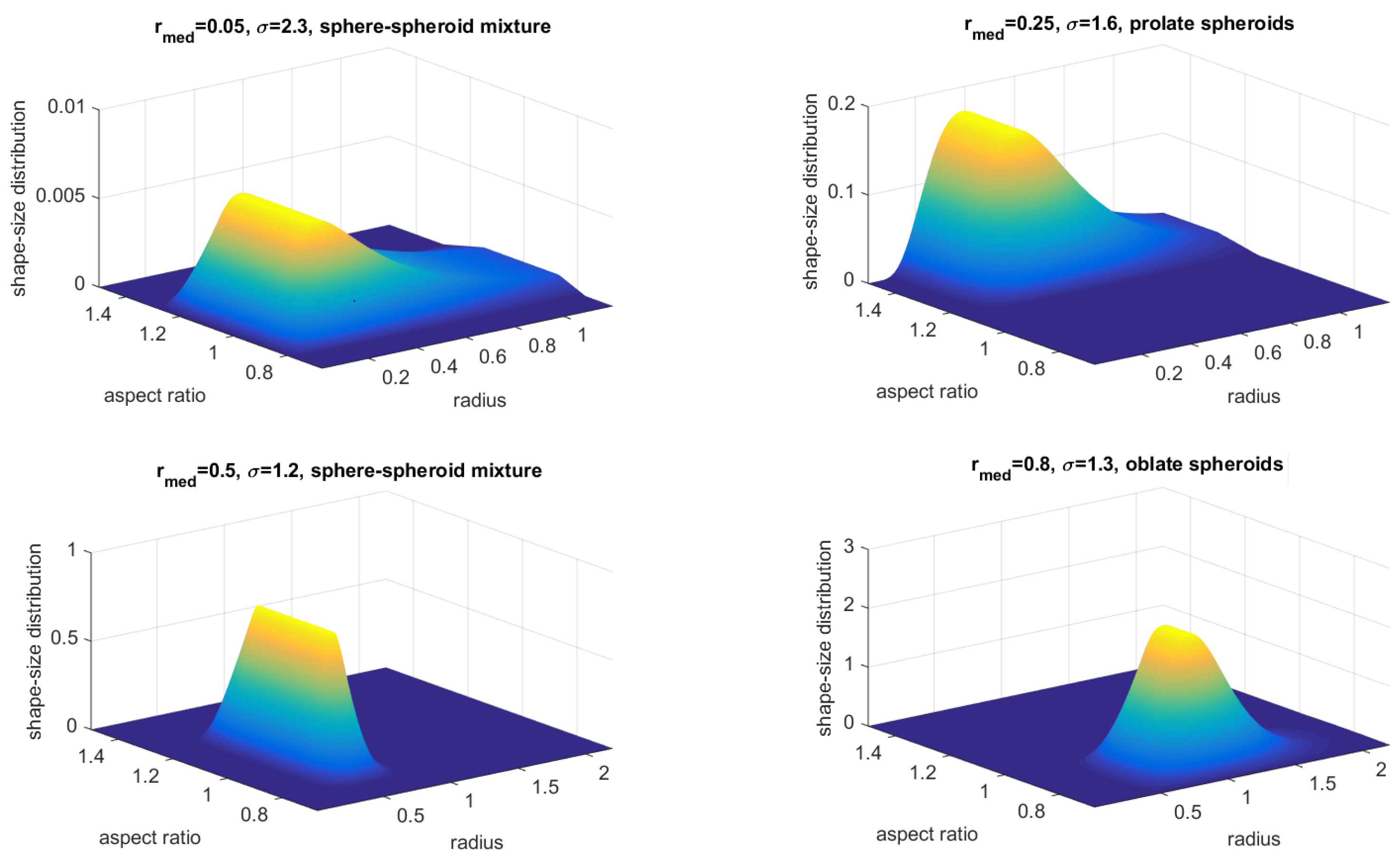
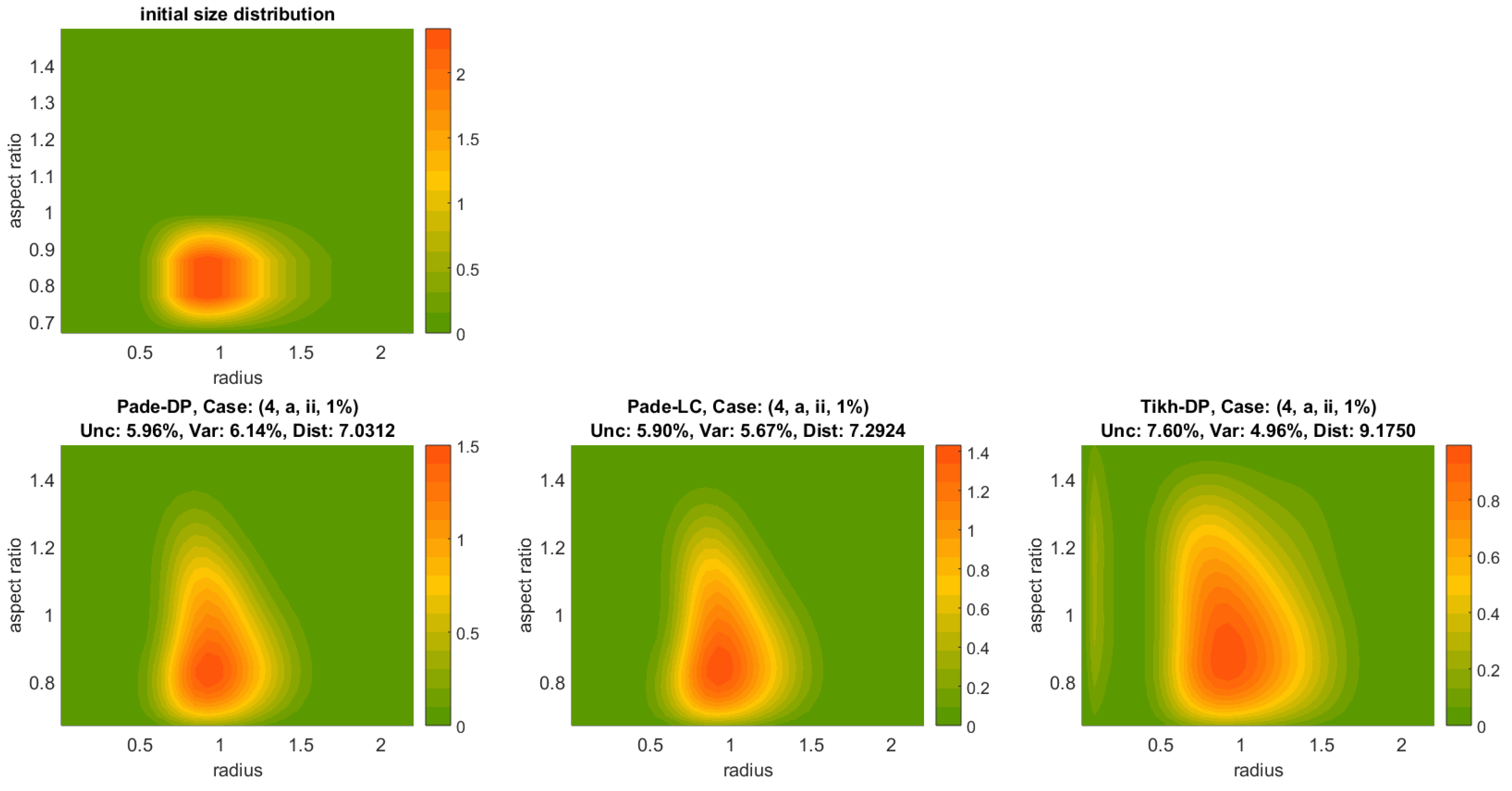
The primary objective of our inversion here is the shape-size distribution $v(r,\eta )$. The first stage in trying to solve Equation (31) is, of course, a discretization, which is done here with projection by quasi-2D collocation as proposed before. There are two other important practical implications here: (i) the determination of the refractive index (m) and (ii) the calculations of the kernel functions (efficiencies). The refractive index is actually an unknown too, and solving for it introduces a highly nonlinear quest. However, in this work, we only investigate several instances of an a priori known refractive index.

The most time-consuming part of solving the model equation is the discretization due to the unprecedented computational expense of the kernel-function calculations. For this reason a precalculated database was created by [36] using the software tool Mieschka. Additionally, it provides an extensive database of scattering quantities for spheroidal geometries, currently also available through an interactive platform of the German Aerospace Center (DLR). Mieschka’s look-up tables include scattering efficiencies for a $6\times 7$ ($\mathrm{Re}\left(m\right)\times \mathrm{Im}\left(m\right)$) refractive index grid (a total of 42 RI values), seven different aspect ratios and a size parameter range $[0.02,40]\mathsf{\mu }$m with a resolution of 0.2. Specifically, the refractive indices and aspect ratios used from the database of Mieschka software [36], are the following:

$$\begin{array}{c}\hfill \begin{array}{cc}\hfill \mathrm{Re}\left(m\right)\in & \{1.33,1.4,1.5,1.6,1.7,1.8\}\hfill \\ \hfill \mathrm{Im}\left(m\right)\in & \{0,0.001,0.005,0.01,0.03,0.05,0.1\}\hfill \\ \hfill \eta \in & \{0.67,0.77,0.87,1,1.15,1.3,1.5\}\hfill \end{array}\end{array}$$

(32)

The resolution gap in the aspect ratio needed for the integrations is handled with interpolation to the nearest neighbor; other interpolation techniques, e.g., cubic interpolation, show only tenuous differences in the discretization outputs.

Although the calculation of the efficiencies for a specific refractive index, size parameter and aspect ratio is already handled by the look-up tables of Mieschka software, we are still left with the interpolation of these functions and the double integration of the discretization procedure, see Equation (28). For this reason, another database was created, this time including the discretization matrices with number of spline points from 3 up to 20 combined with spline degree from 2 up to 6. The spline points for the aspect ratio are fixed to 7, the actual number of different aspect ratio values (Equation (32)). This large collection far exceeds the needs of the present work, covering lots of different discretization dimensions. The integrations involved a two-dimensional Gaussian quadrature integration scheme with a relative tolerance ${10}^{-3}$.

The latter approach is particularly useful for another important reason too. Prior to the regularization, the problem has to be projected in a space of finite dimension, to be able to be solved in the first place. Finding a suitable dimension is the key as shown in [37], and it is often problematic to pick one dimension as a global setting to handle datasets which correspond to very different atmospheric scenarios. Therefore, the mathematical constraint we will use in this work are the spline features (number of spline points and spline degree) which are associated with the dimension of the produced linear system. Previous work done with real-life data in [25,37,38,39] in parallel with several early simulations for this work, showed the benefit of such hybrid algorithms, the concept of which is the leading approach of the present work as well.

After discretizing the model Equation (31), we solve the resulting linear system with regularization, which is the first big step to counteract the ill-posedness of this inverse problem. Having usually no further information about the data error makes it difficult to choose an optimal regularization parameter which will guarantee physical adequacy.

We often encounter a situation where the actual solution coefficients are zero (or nearly zero), but might, nevertheless, turn to negative values due the noise presence (e.g., measurement errors). This is apparently an undesired eventuality from a physical point of view, which we prevent by setting all strictly negative coefficients to zero. This decision is a result of early numerical experiments for this work leading to a superior algorithm performance. Especially for Padé iteration, we apply the non-negativity constraint to the solution in each iteration.

The reader is reminded that the primary unknowns of the resulting linear systems are the spline coefficients of the shape-size distribution (and not the function itself) with respect to the specified projection space.

Algorithm using a fixed refractive index:

• Specify the range of the number of spline points and the range of spline degrees.
• Discretize for every number of spline points, every spline degree and the fixed refractive index. (Use of database of precalculated discretization matrices (T))
• Choose a regularization method and a parameter choice rule to solve the linear systems for a given (error-) dataset (g) applying the non-negativity constraint.
• For all sets of solution coefficients v, make the forward calculation $\tilde{g}=Tv$ and estimate the residual error $\parallel \tilde{g}-g\parallel$.
• Calculate the solutions (shape-size distributions) with respect to the corresponding projection spaces.
• Calculate the mean solution out of a few least-residual solutions.

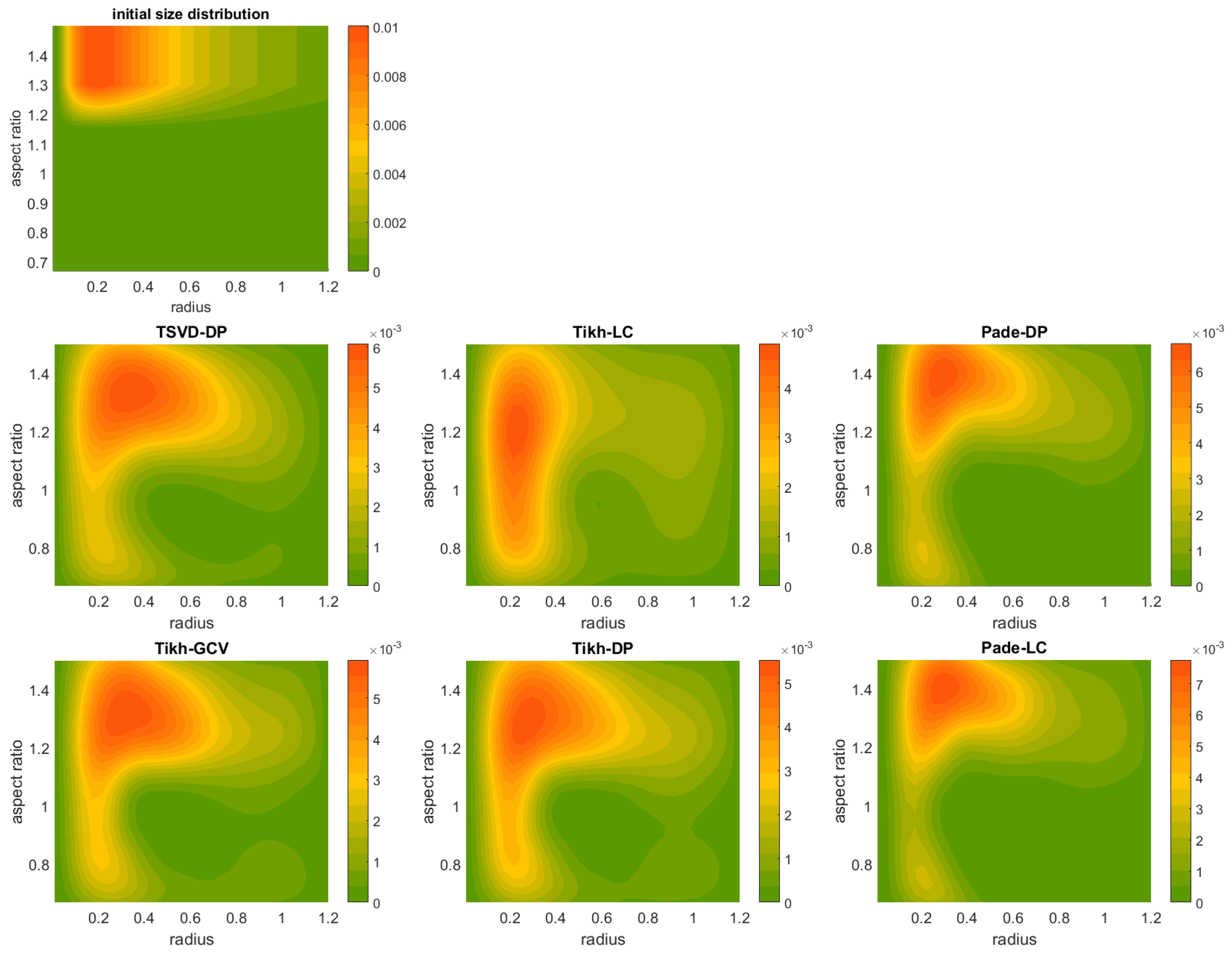
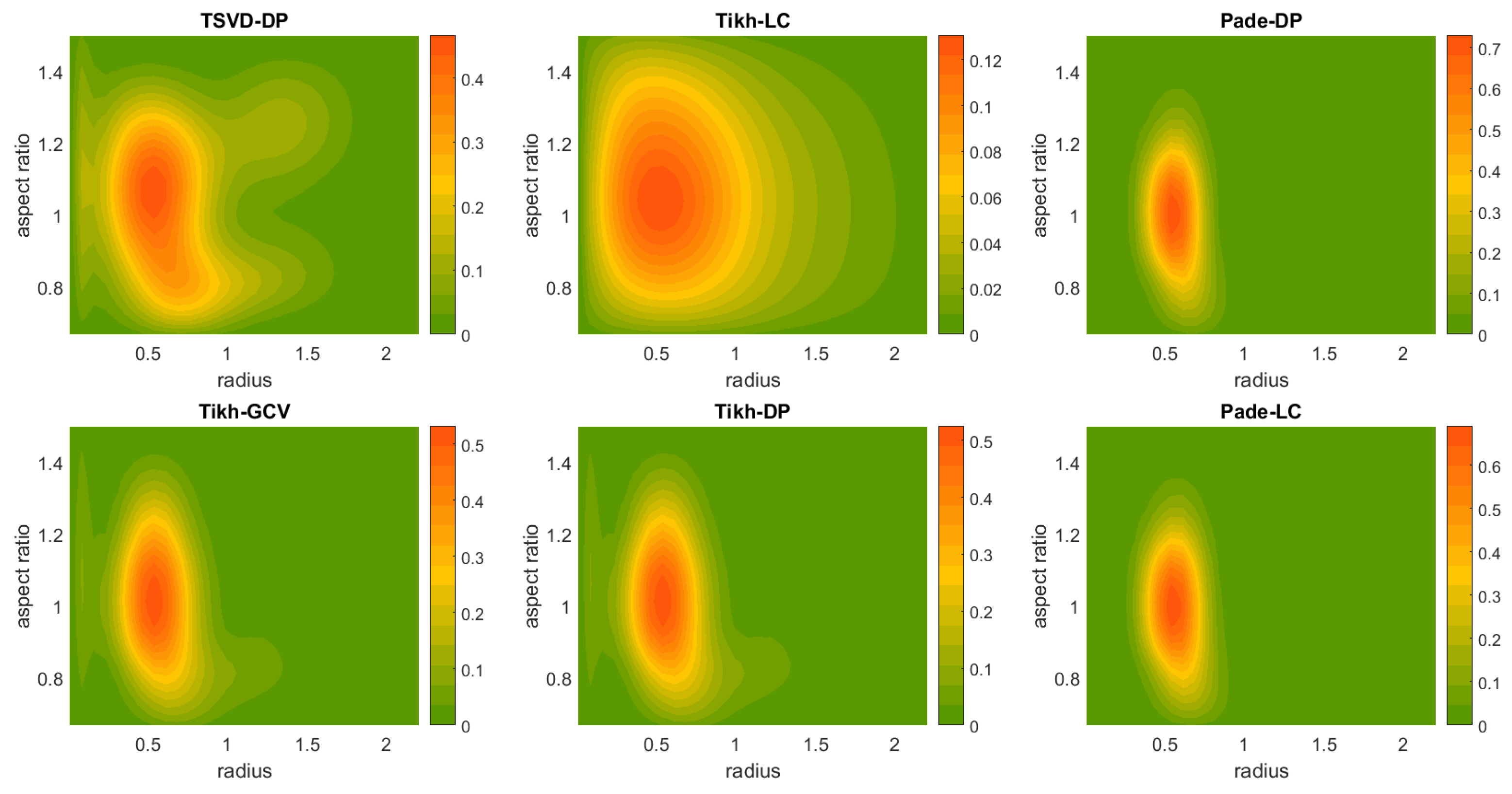
The regularization methods and the parameter choice rules are chosen among the following ones:

• Truncated singular value decomposition with the discrepancy principle (TSVD-DP);
• Tikhonov regularization with the L-curve method (Tikh-LC);
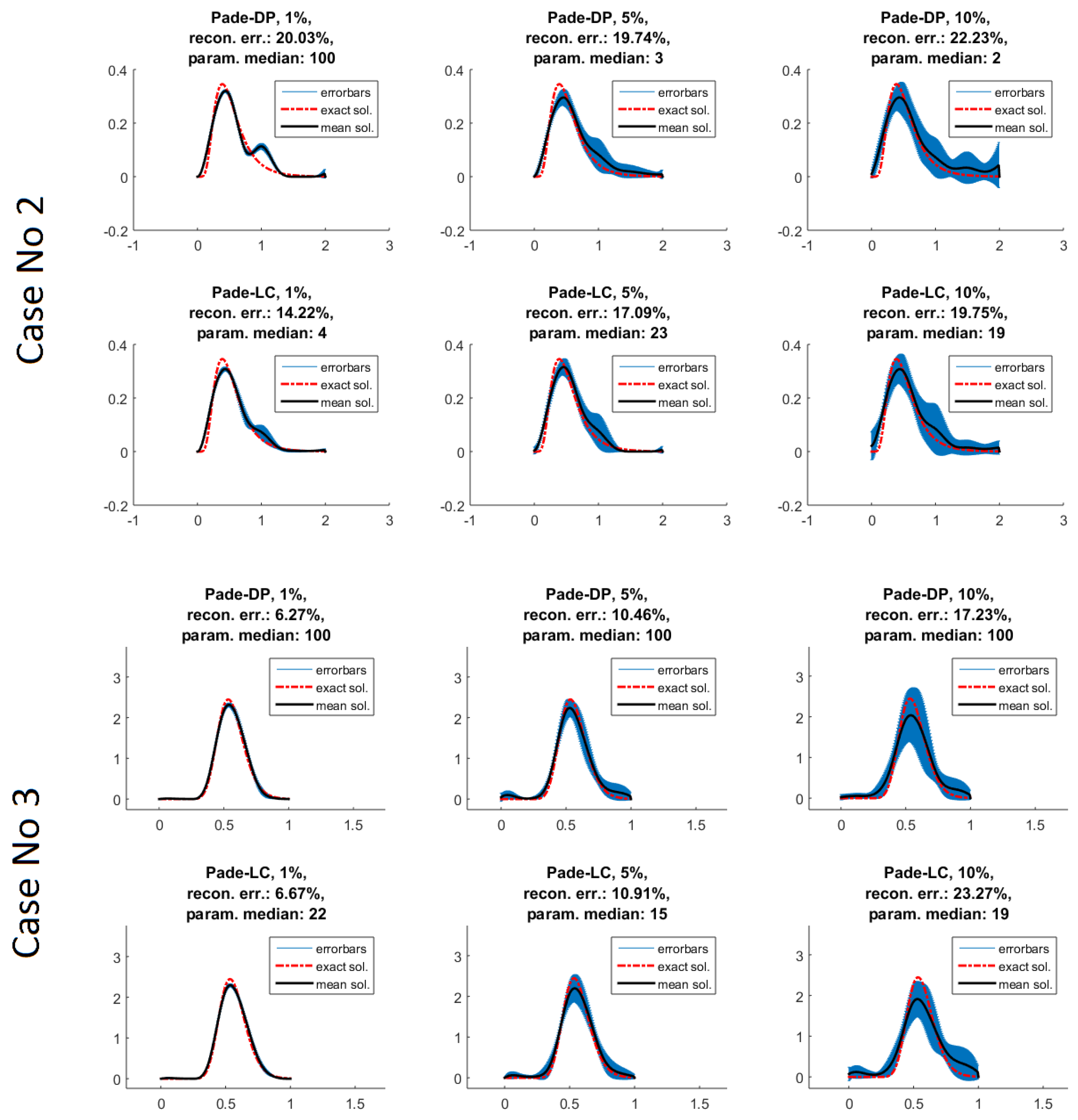
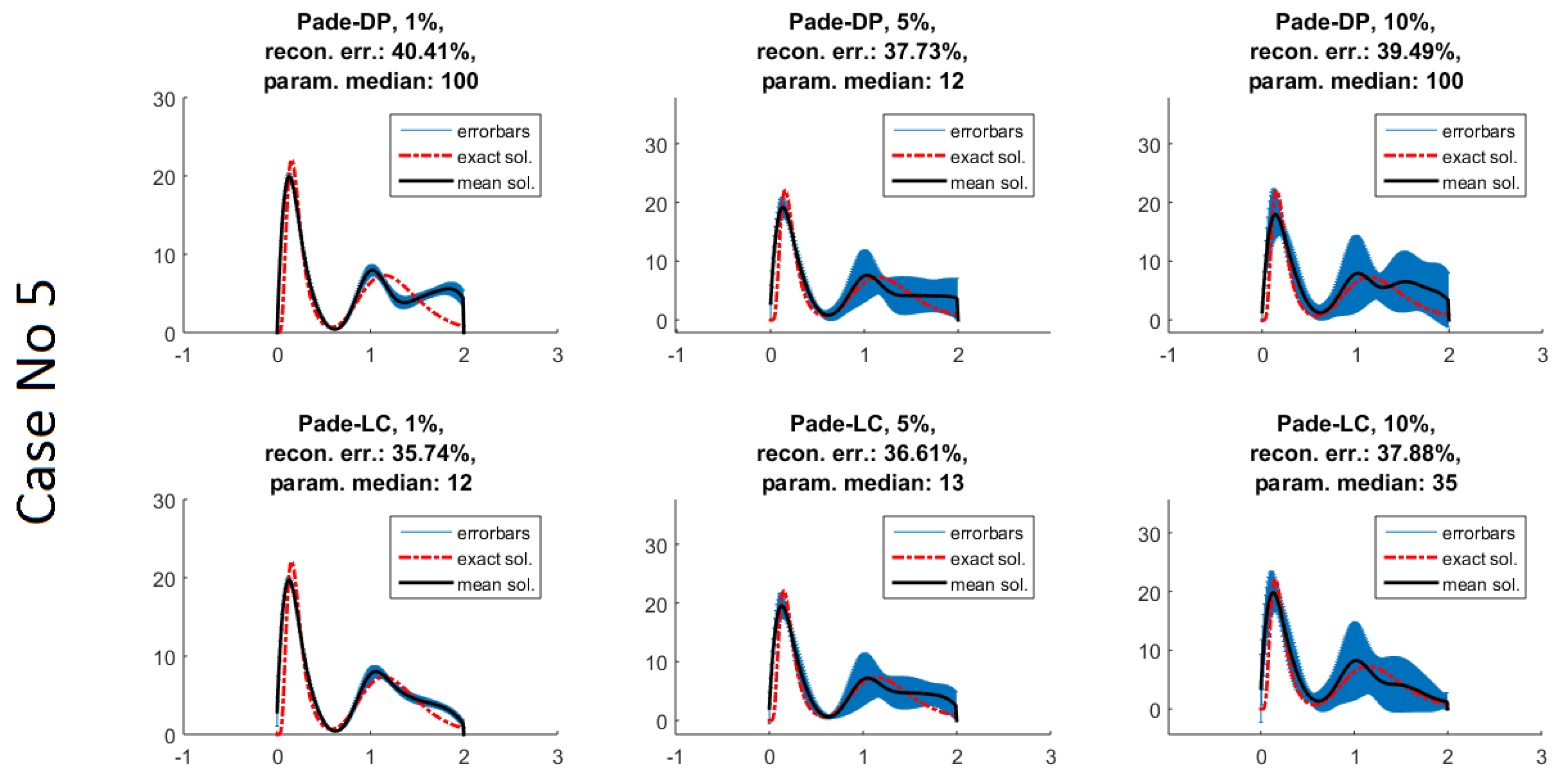
• Padé iteration with the discrepancy principle (Padé-DP);
• Tikhonov regularization with the generalized cross validation method (Tikh-GCV);
• Tikhonov regularization with the discrepancy principle (Tikh-DP); and
• Padé iteration with the L-curve (Padé-LC).

The methods in 1, 2, 4 and 5 are well studied regularization methods and parameter choice rules which have been widely used for the spherical particle model, e.g., [24,25], and it is interesting to see their efficiency for the new spheroidal model as well. Similarly, we investigate the lesser known Padé iteration as a regularization method, first used in the lidar-data inversion by [40], here combined with the discrepancy principle (3), and for the first time with the L-curve method (6). The parameter choice rules are also common in bibliography, and, while they operate very differently, the primary reason for their use here is the presence (DP) or lack of a priori error knowledge (LC, GCV); see the brief review in Section 2.

TSVD-DP (1) is implemented using the theory directly from Section 2.1.1. We start by including all the terms in the SVD-description of the solution and remove them one by one till the discrepancy principle is fulfilled or we arrive at a single term. Apparently, the assumed discrepancy (perhaps multiplied by a safety factor) cannot be smaller than the residual error with all the SVD-terms included. In other words, we cannot demand a better approximation than the best we have.

The Padé approximants (see Equation (26)) for Padé iteration (3, 6) were calculated using a routine implemented by [15], which was integrated in the code. Padé-DP is implemented simply by fixing a maximum number of iterations (MNI) and checking if the assumed discrepancy is interposed between the corresponding residual terms of two successive iterations. The iteration is stopped either by the satisfaction of the DP or by reaching the MNI. For Padé-LC (6), we use a discrete implementation of L-curve with respect to the number of iterations the following way:

• Fix a maximum number of iterations (MNI) m and run Padé iteration for each number $1,\dots ,m$. (m independent times in total);
• Store the residual error $\parallel \tilde{g}{-g\parallel }^2$ and the regularity term ${\parallel v\parallel }^2$ for each number of iterations;
• Build the L-curve with cubic spline interpolation from the points $(\parallel \tilde{g}-g{\parallel }^2,\parallel v{\parallel }^2)$;
• Locate the point of maximum curvature of the L-curve $m^{★}$;
• Take as the solution the output of Padé iteration with $m^{★}$ iterations.

For Tikh-LC (2), Tikh-GCV (4) and Tikh-DP (5), we used modified versions of routines used in the software package Regularization Tools by P.C. Hansen [41].

5. Numerical Simulations of Particle Ensembles

First, we investigate briefly the efficiency of Padé-LC for the atmospheric particle model, but for spherical particles ($\eta =1$), a case that is relatively easier than the spheroidal one. The focus of the simulations here is the reconstruction of the size distribution. We experiment with different atmospheric scenarios artificially produced with the log-normal-distribution parameters and refractive indices shown in

Table 1. Simulation parameters for preliminary tests for spherical particles, $\eta =1$, (nc: number concentration).

Case	Radius Interval	Median Radius	Mode Width	nc	RI
2	$[0.001,2]$	0.25	1.6	1	$1.5+0.01i$
3	$[0.001,1]$	0.5	1.2	1	$1.7+0.05i$
5	$[0.001,1]$	$[0.1,1]$	$[1.6,1.3]$	$[400,1]$	$1.5+0.01i$

.

For this purpose, we conducted the following preliminary synthetic retrievals for a variety of test problems and finally for the inversion of the spherical model with an optical 5-point synthetic dataset $3\beta +2\alpha$. For all inversions, we use the (2,1)-Padé iteration (see (26) for the notation) with a maximum number of 100 iterations and the relaxation parameter set to 100. These values resulted from experience with earlier simulations, and they are also in accordance with findings in [35,42]. The discretization dimension is fixed to 11, considering 9 spline points and 3rd-degree splines. The initial- and retrieved size distributions were derived using a 200-point resolution. The spherical kernel functions were calculated through a Matlab implementation of Bohren and Huffman code [43].

Using these parameters, we create datasets with input white noise 1%, 5% and 10% and repeat the experiment 15 times with different random distribution for each error level. In addition to Padé-LC, we solve also with Padé-DP for comparison and present the results for the cases 2, 3, 5 in Figure 1. The title of each plot shows also the mean reconstruction error and the median of the iteration numbers found in the 15 individual retrievals.

5.1. Results for the Spherical Particle Model

First, let us focus on the cases No. 2 and 3 which involve monomodal log-normal distributions. The first case (Case No. 2) is with medium size and medium absorbing particles ($1.5+0.01i$). Padé-LC continues to have milder artifacts than Padé-DP, obviously due to a better control of the iteration number. The second monomodal-distribution case No. 3 pertaining to very absorbing particles ($1.7+0.05i$) is the most successful for these methods. Indeed, both of them deliver an equivalently precise reconstruction, with Padé-DP being only marginally better for the case of 10% data-error. Moreover, compared to the case 2, we see here the lowest reconstruction errors with respect to any error level.

The last part of numerical experiments involves the much harder task of reconstructing a bimodal size distribution, the last set of plots in Figure 1 related to case No. 5. Experiments involving a large coarse mode and a more silent fine mode (not shown here), are dealt very well by both methods even in the case of large data error. Instead, we include only the more challenging task of a big fine mode and a relatively smaller coarse mode. The methods are struggling to retrieve especially the coarse mode, with Padé-LC prevailing overall. Despite the evident noise for 5 or 10% data error, Padé-LC’s solutions are still following closely enough the pattern of the initial distributions.

We conclude that Padé-LC works generally better than Padé-DP, an advantage apparently attributed to the L-curve method. Indeed, we observe large differences in the median of iterations between LC- and DP-solutions in the vast majority of the cases, see e.g., cases No. 2 and 5 with 1% errors. This result is not taken for granted later on for the non-spherical case where these methods are retested in a much larger scale and since the purpose of the examples here was mainly to demonstrate Padé-LC’s reasonable regularization behavior. In fact, a reconstruction can be very prone to either oversee a mode (mainly coarse) or create artifacts where the distribution is essentially zero. This behavior is hinted e.g., in case No. 5, Padé-DP 1% where an additional mode is being built and then steeply forced to zero. However, the full potential of these methods was dormant since we had a fixed discretization dimension which could ideally handle better these difficulties.

5.2. Results for the Spheroidal Particle Model

5.2.1. Reconstruction of Monomodal Size Distribution

In the following Sections, we perform numerical experiments with artificial data simulating several atmospheric scenarios. These retrievals give valuable insights already used for real-life data from lidar measurements, see [44,45,46]. Our investigations, analyses, and results were realized with a Windows 10 workstation PC of 16 $\mathrm{GB}$ RAM and a 2.40 $\mathrm{GHz}$ quad-core processor.

We assume, as already mentioned, exact knowledge of the refractive index. We will consider 8-point synthetic datasets, i.e., $3{\beta }_{\perp }+3{\beta }_{\parallel }+2\alpha$ (for more details, see [46]) associated with optical products of the most advanced polarization lidars [47] in the present time. The shape-size distribution $v(r,\eta )$ is formed by multiplying a log-normal distribution $v\left(r\right)$ with an aspect ratio distribution $a\left(\eta \right)$

$$v(r,\eta )=v\left(r\right)a\left(\eta \right).$$

(33)

The aspect ratio distribution $a\left(\eta \right)$ is given by the simple model

$$a\left(\eta \right)=\left\{\begin{array}{cc}{p}_1,\hfill & \mathrm{if}\eta ={\eta }_1,\hfill \\ p_2,\hfill & \mathrm{if}\eta ={\eta }_2,\hfill \\ ⋮\hfill & ⋮⋮\hfill \\ p_{\nu },\hfill & \mathrm{if}\eta ={\eta }_{\nu },\hfill \end{array}\right.$$

(34)

where $0\le p_j\le 1$, $j=1,2,\dots ,\nu$ and $p_1+p_2+\dots +p_{\nu }=1$. The selected aspect ratio distributions cover the three most interesting cases: (a) oblate ensembles, (b) sphere-spheroid mixtures and (c) prolate ensembles, see

Table 2. Simulation- and inversion setup with a fixed refractive index. Parameters below the titles “Distribution data generated with”, “Optical data generated with” and “Optical data inverted with” are combined with each other to perform the corresponding action.

Distribution Data Generated with
log-normal distribution
No				1	2	3	4
mode radius ($r_{\mathrm{med}}$) ($\mathsf{\mu }$m)				0.05	0.25	0.5	0.8
mode width ($\sigma$)				2.3	1.6	1.2	1.3
radius range ($\mathsf{\mu }$m)				[0.01, 1.2]	[0.01, 1.2]	[0.01, 2.2]	[0.01, 2.2]
number concentration (nc)				1	1	1	1
aspect ratio distribution
(a) oblate			(b) sphere-spheroid mixture			(c) prolate
$$\left\{\begin{array}{cc}1/2,\hfill & \mathrm{if}\eta =0.77,\hfill \\ 1/2,\hfill & \mathrm{if}\eta =0.87,\hfill \end{array}\right.$$			$$\left\{\begin{array}{cc}1/3,\hfill & \mathrm{if}\eta =0.87,\hfill \\ 1/3,\hfill & \mathrm{if}\eta =1,\hfill \\ 1/3,\hfill & \mathrm{if}\eta =1.15,\hfill \end{array}\right.$$			$$\left\{\begin{array}{cc}1/2,\hfill & \mathrm{if}\eta =1.3,\hfill \\ 1/2,\hfill & \mathrm{if}\eta =1.5,\hfill \end{array}\right.$$
Optical data generated with
refractive index
(i) 1.33 + 0.001i		(ii) 1.4 + 0.005i		(iii) 1.5 + 0.01i	(iv) 1.6 + 0.001i		(v) 1.7 + 0.05i
number of spline points
6	7	8	9	10	11	12	13	14
spline degrees
			2	3	4	5
relative error level ($\times 15$ repetitions)
			1%	5%	10%

for the specific used values. The associated case-aspect ratios (${\eta }_j,j=1,2,\dots ,\nu$) are selected from the exact available ones in Mieschka’s database, see Equation (32). The radius ranges are $[0.01,1.2]$ or $[0.01,2.2]$ both for the distributions and for the integration, and the aspect ratio range is $[0.67,1.5]$. Figure 2 shows some examples of shape-size distributions from Table 2.

The combination of the (four) log-normal distributions with the (three) aspect ratio distributions from Table 2 yield an effective-radius range of 0.26 to 0.95 $\mathsf{\mu }$m. The aforementioned sizes cover many interesting cases of aerosol particle ensembles and fall within the range of fine and medium-coarse dust-like particles but do not span, of course, the whole physically occurring range.

For the discretization of the model Equation (31), the refractive index and the projected dimension (splines) are necessary. The fixed refractive index for the scattering efficiencies takes the values $1.33+0.001i,1.4+0.005i,1.5+0.01i,1.6+0.001i$ and $1.7+0.05i$ (one at a time). The number of spline points and spline degrees take over values from the ranges 6 up to 14 and 2 up to 5, respectively, resulting in projection dimensions from 7 up to 18. The lowest dimension 7 used here was found also in [37] to be marginally sufficient, while a larger dimension than 18 might result in a systematic behavior in the retrieval because the linear systems end up highly underdetermined.

Once the optical dataset is created with a forward run of Equation (31), we add to it Gaussian white noise, with relative error levels 1%, 5% and 10%. Every dataset is randomly generated 15 times for the same error level. Finally, the produced linear systems are solved with the regularization methods 1–6.

The discrepancy $\delta$ for TSVD-DP, Padé-DP and Tikh-DP is automatically computed for a simulation from the known error level ($ϵ$) by $\delta =ϵ\parallel g\parallel$, where g is the error-free dataset, and the safety factor is set to be unit. The $(m,n)$-Padé iteration scheme used here is $(2,1)$, which was found suitable for regularization in [15,38,40,42]. The maximum number of iterations for Padé-DP/-LC is fixed to 100, and the relaxation parameter is fixed to 100.

A straightforward observation from Figure 3, Figure 4, Figure 5, Figure A1 and Figure A2 (see Appendix C) is that TSVD-DP and Tikh-GCV/LC/DP are the least efficient methods and may be ruled out. The most probable cause of this behavior is the overestimation or underestimation of the regularization parameter leading to oversmoothed or undersmoothed solutions.

There are only small differences in accuracy between Padé-DP and Padé-LC, mostly in favor of Padé-LC which occasionally amounts to a better distribution reconstruction than the one produced by Padé-DP which was already observed in the previous spherical case study.

Figure 3 and Figure 4 show the error-level evolution of the produced reconstruction by Padé-DP, Padé-LC and Tikh-DP (left to right) for the cases (2, c, iii) and (4, a, ii) respectively for 1% (2nd row) and 10% (3rd row) error level; the initial shape-size distribution is shown in the uppermost plots for both figures. In addition, the triple (Unc, Dist, Var), for explanation see Appendix B, is given in the title of each reconstruction. Each solution space here owns 36 solutions (9 splines-point numbers × 4 spline degrees), five of which are selected as the least-residual error solutions and are involved in the variability percentage. Padé-DP and Padé-LC achieve a more accurate reconstruction than Tikh-DP in both cases (2, c, iii) and (4, a, ii) and both error levels. Indeed, Padé iteration has less pronounced artifacts than Tikh-DP and preserves the location of the peak (see also colorbars) and its width better. For instance, the case (2, c, iii, 1%) in Figure 3 Dist is larger for Tikh-DP and the reconstruction has a stronger spread in the radius axis and more artifacts in the bottom of the graph. Padé-LC achieves a much better reconstruction for the same case but 10% error level; see the lowermost panel of Figure 3, but it has a dubious uncertainty (Unc) of 66.45%, which is more than twice the ones of Padé-DP and Tikh-DP. The case (4, a, ii) in Figure 4 essentially reconfirms the situation in another setting. The Tikh-DP reconstruction presents much stronger elongation in the aspect-ratio axis as well as the radius axis, and there is also some otherwise negligible noise in the beginning (leftmost) of the graph. However, in the case of a 10% error level, there is a reduced chance of ∼$50\%$ (Unc) from the side of Padé-DP/-LC of reaching this accuracy, which is much more than the one of Tikh-DP (23.50%), see the lowermost panel of Figure 4. Furthermore, the variability is considerably lower for Tikh-DP. However, a simple rough calculation for the worst-case scenario (high deviation from the average accuracy) for Padé iteration accounting both Var and Unc shows that it is still better than the one of Tikh-DP, which is the rule for many of the cases.

There is a milder but noteworthy competition between Padé-DP and Padé-LC in distribution reconstructions mostly expressed for 5% or 10% error level. Figure 5, shows several examples of reconstructions for a comparison between Padé-DP and Padé-LC, through which we can also see noisy or less trustworthy outcomes for both methods. For instance, focusing on the uppermost row of plots, i.e., the case (2, c, i, 5%), Padé-LC demonstrates again better accuracy but much higher uncertainty (Unc: 51.54%) than Padé-DP (Unc: 13.81%), which essentially fails to capture the shape of the initial distribution in greater detail. We note that there are plenty of cases with very smooth and nice distribution results that are not shown here, but instead the chosen cases cover mostly difficult encounters for Padé iteration, which may be of practical interest in a real application. Evidently a high error level damages the reconstructions very distinctly. The mildest effect is expressed through the aforementioned spread in radius- or aspect ratio axis, while stronger noise involves additional “modes” (artifacts), see e.g., the lowermost panel of Figure 3. However, it is important to realize that, in an experimental case (real data), multimodality is quite a probable scenario and our intuition about what is noise or a real extra mode has to be conformed accordingly. As a general remark, the location of the peak in the radius axis is best reproduced, as compared to the (radius) mode width, the aspect ratio width and the height of the peak, i.e., the volume distribution (colorbar). Indeed, even in cases of mistreatment of the shape (aspect ratio), the location of peak in the radius axis is still obtained, see e.g., the uppermost or lowermost panel of Figure 5. The plots in Figure 4 for Padé iteration correspond to the best we can do for a case with oblate spheroids; most often, the distributions are falsely shifted upwards, resembling those of the sphere-spheroid mixture. The refractive index obviously plays a crucial role in the inversion even if the initial shape- and size settings are the same, since the kernel functions impose different levels of smoothing depending on its value. We can see this through the examples on the 2nd and 3rd row of plots in Figure 5 referring to the cases (3, c, iv, v, 10%). These instances show the reconstruction of same shape-size distribution for the extreme cases of weakly absorbing particles ($\mathrm{RI}:1.6+0.001i$) and very absorbing particles ($\mathrm{RI}:1.7+0.05i$), illustrating the infiltration of noise and the enhanced difficulty for an approximation associated with the absorbing case.

5.2.2. Reconstruction of Bimodal Size Distribution

In this Section, we would like to show the potential of our approach in retrieving bimodal shape-size distributions, restricting to reconstructions produced by Padé-DP. Multimodality in a two-dimensional aerosol distribution has never been studied, as a result of the mere absence of a 2D-representation of the distribution itself from contemporary bibliography for the sake of simplicity. Indeed, in order to even build a shape-size distribution of desired modes (location, peak, etc), experience of some level is required as compared to the case of a usual size distribution since there is no standard procedure and the additional dimension (aspect ratio) expands significantly the possible outcomes. The construction of such distributions is based here again on simple multiplication of independent log-normal size distributions and aspect ratio distributions. The parameters used to create the synthetic data and distributions are shown in

Table 3. Simulation setup for the reconstruction of bimodal shape-size distributions (BMD) with a fixed refractive index and 1% error level. The following combinations were used: BMD 1: (1, a, iii), BMD 2: (2, a, iii), BMD 3: (3, e, ii), BMD 4: (4, d, i), BMD 5: (3, b, iii), BMD 6: (4, c. i).

log-normal distribution
No	1	2	3	4	5	6
median radius ($\mathsf{\mu }$m)	$[0.05,1.4]$	$[0.2,1]$	$[0.5,1.6]$	$[0.8,1.7]$	0.5	0.8
mode width	$[2.3,1.2]$	$[1.6,1.4]$	$[1.3,1.2]$	$[1.2,1.2]$	1.2	1.4
radius range ($\mathsf{\mu }$m)	$[0.01,2.2]$	$[0.01,2.2]$	$[0.01,2.2]$	$[0.01,2.2]$	[0.01, 2.2]	[0.01, 2.2]
number concentration (nc)	$[600,1]$	$[30,1]$	$[12,1]$	$[6,1]$	1	1
aspect ratio distribution
	$$\left(a\right)\left\{\begin{array}{cc}1/2,\hfill & \mathrm{if}\eta =0.87,\hfill \\ 1/2,\hfill & \mathrm{if}\eta =1,\hfill \end{array}\right.$$		$$\left(b\right)\left\{\begin{array}{cc}1/3,\hfill & \mathrm{if}\eta =0.77,\hfill \\ 2/3,\hfill & \mathrm{if}\eta =1.3,\hfill \end{array}\right.$$		$$\left(c\right)\left\{\begin{array}{cc}1/3,\hfill & \mathrm{if}\eta =0.87,\hfill \\ 2/3,\hfill & \mathrm{if}\eta =1.3,\hfill \end{array}\right.$$
	$$\left(d\right)\left\{\begin{array}{cc}1/3,\hfill & \mathrm{if}\eta =0.87,\hfill \\ 1/3,\hfill & \mathrm{if}\eta =1,\hfill \\ 1/3,\hfill & \mathrm{if}\eta =1.15,\hfill \end{array}\right.$$		$$\left(e\right)\left\{\begin{array}{cc}1/2,\hfill & \mathrm{if}\eta =1.3,\hfill \\ 1/2,\hfill & \mathrm{if}\eta =1.5,\hfill \end{array}\right.$$
refractive index
	(i) 1.33 + 0.001i		(ii) 1.4 + 0.005i		(iii) 1.5 + 0.01i

(BMD: 1–4). We will investigate shape-size distributions which have two distinct modes either on the radius axis formed by a bimodal log-normal distribution (BMD: 1–4) or on the aspect ratio axis (BMD: 5, 6) with greater emphasis on the latter.

The new inversion examples were ran 15 times for 1% error level, choosing as usual 5 best solutions (out of 36) for each run and the reconstruction plots are shown in Figure 6 and Figure 7 containing also information about the involved uncertainties in their titles. The top first and second panels of Figure 6 depict examples of a fixed mixture of oblate and spherical particles combined with very diverse bimodal log-normal distributions, each of which marrying fine (BMD 1) or very fine absorbing particles (BMD2) with coarse ones, see Table 3. In both of these cases, the reconstructions are remarkably good at making out the different modes not only locating the peaks but also the transition between the modes. This detail is especially pronounced in the BMD 2, see the smaller 3D plots within the main plots. The radius-width and the aspect ratio width are reproduced with good accuracy as well, with BMD 1 allowing more noise into the plot. The third plot from the top of Figure 6 (BMD 3) relates to a case of prolate particles where both modes pertain to coarse particles. The reconstruction faces greater difficulty but all in all has similar characteristics, i.e., identifying two modes which overall resemble the initial trends. The second mode (right), however, appears to be noisier, and its peak is shifted on downward and right, and we further observe a height suppression of the peaks and some artifacts in the bottom of the graph. The modes on the last plot (BMD 4) pertain to very coarse particles combined with the sphere–spheroid mixture used extensively in the previous simulations. Here, in addition to the overall good response of the method, we can see that the reconstruction senses also the small height difference between the mode peaks. The second mode (again) suffers bigger errors but within a reasonable level.

Shape bimodality appears to be more problematic, probably as a result of the limited access we have on kernel values with respect to the aspect ratio. Figure 7 shows our attempts to reproduce two atmospheric settings (BMD 5, 6 in Table 3) of a fixed particle size combined with a mixed ensemble consisting of oblate and prolate particles. The example BMD 5 (upper panel) shows correct identification and detection of the two modes (location, radius width), but the strength of the modes (peak heights) is reversed. The second example, BMD 6 (lower panel), pertains to weakly absorbing particles (in contrast to BMD 5) with much larger radius width. The relative strength of modes and their separation is well felt by the reconstruction, but the upper mode is noisy and the peak of the lower mode is shifted downward. Bimodal distributions with vicinal shape modes, e.g., using a prolate ensemble with $\eta =1.15$ and $\eta =1.5$, are often mistreated by the inversion, showing the two modes merged to a single wider one and thus revealing a shortcoming in sensitivity. We should underline that the right choice of spline number and degree by the algorithm seems to be more delicate when there is an aspect-ratio-related bimodality. In this case, further simulations showed that a smaller projection dimension is often needed, i.e., a small number of spline points and/or degree, in order to better identify the two modes.

6. Conclusions and Outlook

Starting with the common Fredholm integral equation, we presented the theoretical requirements to achieve a stable generalized solution. The SVD of the Fredholm operator provided an insightful connection of the inherent instability of these inverse problems to the existence of very small singular values which potentially magnify noisy components of the solution. This motivated the definition of regularizers, in particular, through the useful framework of filter functions whose regularizing effect is reduced to a small checklist of simple properties. The latter was shown to be satisfied by the family of Runge–Kutta iterative methods, from which we chose the (2,1)-Padé iterative regularizer to be among the methods for our numerical experiments with synthetic data pertaining to different atmospheric scenarios. First, we established the robustness of a new data-driven method combining (2,1)-Padé with a L-curve method for the spherical particle case through reconstructions of 1D (volume) size distributions. Expanding the Fredholm integral model to a quasi-2D one, in order to accommodate the spheroidal particle approximation, brought about a more complex and nuanced particle distribution function, i.e., the shape-size distribution, which became our measure for a larger round of method comparisons. (2,1)-Padé method stood out among the other traditional methods, with the LC version (L-curve) being relatively more accurate and the DP version (discrepancy principle) being more stable. Accounting for the fact that estimates of measurement data error (necessary for DP) are mostly absent in applications, the purely data-driven method Padé-LC is a favorable choice. Finally, we went on to reconstruct limited cases of bimodal shape-size distributions with remarkable fidelity, pushing at the same time the limits of our approach. Putting aside the substantial complexity imposed by the spheroidal particle approximation, e.g., numerical convergence of kernel functions, quasi-2D discretization, 2D integrations for the forward model, unfamiliar interpretation of a shape-size distribution, etc., there are evident practical limitations to this approach for it to become fully operational. These involve mostly the restrictions of the scattering database limiting the refractive indices to a characteristic but quite small grid and the aspect ratio range to a few values. Limitations on the so-called size parameter ($2\ast \pi \ast r/\lambda$) also force the radius range to account for particles up to 2.2 $\mathsf{\mu }$m and might also lead to misidentification or disruption of distribution modes as shown. These are all topics that would potentially improve the performance of our method and need to be taken into account in future studies along with the use of real-life lidar measurements. Nonetheless, this study marks a more mature point for the handling of the non-spherical microphysical retrieval problem bringing back to the discussion the role of shape, in an active manner, as a variable of the particle distribution missing from other approaches.

References

1. Rieder, A. Runge–Kutta integrators yield optimal regularization schemes. Inverse Probl. 2005, 21, 453–471. [Google Scholar] [CrossRef]
2. Pornsawad, P.; Böckmann, C.; Panitsupakamon, W. The Levenberg–Marquardt regularization for the backward heat equation with fractional derivative. Electron. Trans. Numer. Anal. 2022, 57, 67–79. [Google Scholar] [CrossRef]
3. Böckmann, C.; Pornsawad, P. Iterative Runge–Kutta-type methods for nonlinear ill-posed problems. Inverse Probl. 2008, 24, 025002. [Google Scholar] [CrossRef] [Green Version]
4. Pornsawad, P.; Böckmann, C. Convergence rate analysis of the first-stage Runge–Kutta-type regularizations. Inverse Probl. 2010, 26, 035005. [Google Scholar] [CrossRef]
5. Pornsawad, P.; Resmerita, E.; Böckmann, C. Convergence Rate of Runge–Kutta-Type Regularization for Nonlinear Ill-Posed Problems under Logarithmic Source Condition. Mathematics 2021, 9, 1042. [Google Scholar] [CrossRef]
6. Zhao, Y.; Mathé, P.; Lu, S. Convergence Analysis of Asymptotical Regularization and Runge–Kutta Integrators for Linear Inverse Problems under Variational Source Conditions. CSIAM Trans. Appl. Math. 2020, 1, 693–714. [Google Scholar] [CrossRef]
7. Hadamard, J. Lectures on the Cauchy Problem in Linear Partial Differential Equations; Yale University Press: New Haven, CT, USA, 1923. [Google Scholar]
8. Nashed, M. A New Approach to Classification and Regularization of ILL-Posed Operator Equations. In Inverse and Ill-Posed Problems; This Research Was Partially Supported by the United States Army Research Office under Grant DAAG-29-83-K-0109; Engl, H.W., Groetsch, C., Eds.; Academic Press: Cambridge, MA, USA, 1987; pp. 53–75. [Google Scholar] [CrossRef]
9. Baumeister, J.; Leitão, A. Topics in Inverse Problems; Publicações Matemáticas do IMPA: Rio de Janeiro, Brazil, 2005. [Google Scholar]
10. Kress, R. Linear Integral Equations; Applied Mathematical Sciences; Springer: New York, NY, USA, 1999. [Google Scholar]
11. Tikhonov, A.N.; Arsenin, V.Y. Solution of ILL-Posed Problems; Winston: Washington, DC, USA, 1977. [Google Scholar]
12. Engl, H.; Hanke, M.; Neubauer, A. Regularization of Inverse Problems; Mathematics and Its Applications; Springer: Dordrecht, The Netherlands, 2000. [Google Scholar]
13. Butcher, J.C. Coefficients for the study of Runge–Kutta integration processes. J. Aust. Math. Soc. 1963, 3, 185–201. [Google Scholar] [CrossRef] [Green Version]
14. Böckmann, C. Runge–Kutta Type Methods for Ill–Posed Problems and the Retrieval of Aerosol Size Distributions. PAMM Proc. Appl. Math. Mech. 2002, 1, 486–487. [Google Scholar] [CrossRef]
15. Kirsche, A. Regularisierungsverfahren. Entwicklung, Konvergenzuntersuchung und optimale Anpassung für die Fernerkundung. Ph.D. Thesis, University of Potsdam, Potsdam, Germany, 2007. [Google Scholar]
16. Lawson, C.L.; Hanson, R.J. Solving Least Squares Problems; Society for Industrial and Applied Mathematics: Philadelphia, PA, USA, 1974; Volume 161. [Google Scholar]
17. Hansen, P.C. Analysis of Discrete Ill-Posed Problems by Means of the L-Curve. SIAM Rev. 1992, 34, 561–580. [Google Scholar] [CrossRef]
18. Hansen, P.C. The L-Curve and its Use in the Numerical Treatment of Inverse Problems. In Computational Inverse Problems in Electrocardiology; Advances in Computational Bioengineering; Johnston, P., Ed.; WIT Press: Southampton, UK, 2000; pp. 119–142. [Google Scholar]
19. Stone, M. Cross-Validatory Choice and Assessment of Statistical Predictions. J. R. Stat. Soc. Ser. B 1974, 36, 111–147. [Google Scholar] [CrossRef]
20. Kirsche, A.; Böckmann, C. Rational approximations for ill-conditioned equation systems. Appl. Math. Comput. 2005, 171, 385–397. [Google Scholar] [CrossRef]
21. Kirsche, A.; Böckmann, C. Padé iteration method for regularization. Appl. Math. Comput. 2006, 180, 648–663. [Google Scholar] [CrossRef]
22. Korras-Carraca, M.B.; Gkikas, A.; Matsoukas, C.; Hatzianastassiou, N. Global Clear-Sky Aerosol Speciated Direct Radiative Effects over 40 Years (1980–2019). Atmosphere 2021, 12, 1254. [Google Scholar] [CrossRef]
23. Ansmann, A.; Müller, D. Lidar and Atmospheric Aerosol Particles. In Lidar: Range-Resolved Optical Remote Sensing of the Atmosphere; Weitkamp, C., Ed.; Springer: New York, NY, USA, 2005; pp. 105–141. [Google Scholar] [CrossRef]
24. Müller, D.; Wandinger, U.; Ansmann, A. Microphysical particle parameters from extinction and backscatter lidar data by inversion with regularization: Simulation. Appl. Opt. 1999, 38, 2358–2368. [Google Scholar] [CrossRef] [PubMed]
25. Böckmann, C. Hybrid regularization method for the ill-posed inversion of multiwavelength lidar data in the retrieval of aerosol size distributions. Appl. Opt. 2001, 40, 1329–1342. [Google Scholar] [CrossRef] [PubMed]
26. Samoiliva, S.V.; Penner, I.E.; Balin, Y.S. Separate retrieval of microphysical characteristics in aerosol fractions from laser sensing data. J. Quant. Spectrosc. Radiat. Transf. 2022, 285, 108168. [Google Scholar] [CrossRef]
27. Sorrentino, A.; Sannino, A.; Spinelli, N.; Piana, M.; Boselli, A.; Tontodonato, V.; Castellano, P.; Wang, X. A Bayesian parametric approach to the retrieval of the atmospheric number size distribution from lidar data. Atmos. Meas. Tech. 2022, 15, 149–164. [Google Scholar] [CrossRef]
28. Dubovik, O.; Sinyuk, A.; Lapyonok, T.; Holben, B.N.; Mishchenko, M.; Yang, P.; Eck, T.F.; Volten, H.; Muñoz, O.; Veihelmann, B.; et al. Application of spheroid models to account for aerosol particle nonsphericity in remote sensing of desert dust. J. Geophys. Res. Atmos. 2006, 111, D11208. [Google Scholar] [CrossRef]
29. Veselovskii, I.; Dubovik, O.; Kolgotin, A.; Lapyonok, T.; Di Girolamo, P.; Summa, D.; Whiteman, D.N.; Mishchenko, M.; Tanré, D. Application of randomly oriented spheroids for retrieval of dust particle parameters from multiwavelength lidar measurements. J. Geophys. Res. Atmos. 2010, 115, JD014139. [Google Scholar] [CrossRef] [Green Version]
30. Böckmann, C.; Osterloh, L. Runge–Kutta type regularization method for inversion of spheroidal particle distribution from limited optical data. Inverse Probl. Sci. Eng. 2014, 22, 150–165. [Google Scholar] [CrossRef]
31. Tesche, M.; Kolgotin, A.; Haarig, M.; Burton, S.P.; Ferrare, R.A.; Hostetler, C.A.; Müller, D. 3 + 2 + X: What is the most useful depolarization input for retrieving microphysical properties of non-spherical particles from lidar measurements using the spheroid model of Dubovik et al. (2006)? Atmos. Meas. Tech. 2019, 12, 4421–4437. [Google Scholar] [CrossRef] [Green Version]
32. Chaikovsky, A.; Dubovik, O.; Holben, B.; Bril, A.; Goloub, P.; Tanré, D.; Pappalardo, G.; Wandinger, U.; Chaikovskaya, L.; Denisov, S.; et al. Lidar-Radiometer Inversion Code (LIRIC) for the retrieval of vertical aerosol properties from combined lidar/radiometer data: Development and distribution in EARLINET. Atmos. Meas. Tech. 2016, 9, 1181–1205. [Google Scholar] [CrossRef] [Green Version]
33. Kirby, M.; Sirovich, L. Application of the Karhunen-Loève procedure for the characterization of human faces. IEEE Trans. Pattern Anal. Mach. Intell. 1990, 12, 103–108. [Google Scholar] [CrossRef] [Green Version]
34. Van de Hulst, H.C. Light Scattering by Small Particles; John Wiley & Sons: New York, NY, USA, 1957. [Google Scholar]
35. Osterloh, L. Retrieving Aerosol Microphysical Properties from Multiwavelength Lidar Data. Ph.D. Thesis, Potsdam University, Potsdam, Germany, 2011. [Google Scholar]
36. Rother, T.; Kahnert, M. Electromagnetic Wave Scattering on Nonspherical Particles; Springer: New York, NY, USA, 2014. [Google Scholar] [CrossRef]
37. Samaras, S.; Nicolae, D.; Böckmann, C.; Vasilescu, J.; Binietoglou, I.; Labzovskii, L.; Toanca, F.; Papayannis, A. Using Raman-lidar-based regularized microphysical retrievals and Aerosol Mass Spectrometer measurements for the characterization of biomass burning aerosols. J. Comput. Phys. 2015, 299, 156–174. [Google Scholar] [CrossRef]
38. Osterloh, L.; Böckmann, C.; Nicolae, D.; Nemuc, A. Regularized inversion of microphysical atmospheric particle parameters: Theory and application. J. Comput. Phys. 2013, 237, 79–94. [Google Scholar] [CrossRef]
39. Osterloh, L.; Pérez, C.; Böhme, D.; Baldasano, J.M.; Böckmann, C.; Schneidenbach, L.; Vicente, D. Parallel software for retrieval of aerosol distribution from lidar data in the framework of EARLINET-ASOS. Comput. Phys. Commun. 2009, 180, 2095–2102. [Google Scholar] [CrossRef]
40. Böckmann, C.; Kirsche, A. Iterative regularization method for lidar remote sensing. Comput. Phys. Commun. 2006, 174, 607–615. [Google Scholar] [CrossRef]
41. Hansen, P.C. Discrete Inverse Problems: Insight and Algorithms; Society for Industrial and Applied Mathematics: Philadelphia, PA, USA, 2010; Volume 7. [Google Scholar]
42. Osterloh, L.; Böckmann, C.; Mamouri, R.E.; Papayannis, A. An adaptive base point algorithm for the retrieval of aerosol microphysical properties. Open Atmos. Sci. J. 2011, 5, 61–73. [Google Scholar] [CrossRef]
43. Bohren, C.F.; Huffman, D.R. Absorption and Scattering of Light by Small Particles; Wiley: New York, NY, USA, 1983. [Google Scholar]
44. Soupiona, O.; Papayannis, A.; Kokkalis, P.; Foskinis, R.; Sánchez Hernández, G.; Ortiz-Amezcua, P.; Mylonaki, M.; Papanikolaou, C.A.; Papagiannopoulos, N.; Samaras, S.; et al. EARLINET observations of Saharan dust intrusions over the northern Mediterranean region (2014–2017): Properties and impact on radiative forcing. Atmos. Chem. Phys. 2020, 20, 15147–15166. [Google Scholar] [CrossRef]
45. Soupiona, O.; Samaras, S.; Ortiz-Amezcua, P.; Böckmann, C.; Papayannis, A.; Moreira, G.; Benavent-Oltra, J.; Guerrero-Rascado, J.; Bedoya-Velasquez, A.; Olmo, F.; et al. Retrieval of optical and microphysical properties of transported Saharan dust over Athens and Granada based on multi-wavelength Raman lidar measurements: Study of the mixing processes. Atmos. Environ. 2019, 214, 116824. [Google Scholar] [CrossRef]
46. Samaras, S. Microphysical Retrieval of Non-Spherical Aerosol Particles Using Regularized Inversion of Multi-Wavelength Lidar Data. Ph.D. Thesis, Potsdam University, Potsdam, Germany, 2016. [Google Scholar]
47. Weitkamp, C. Lidar: Range-Resolved Optical Remote Sensing of the Atmosphere; Springer Series in Optical Sciences; Springer: Berlin/Heidelberg, Germany, 2005. [Google Scholar]
48. De Boor, C. A Practical Guide to Splines; Springer: New York, NY, USA, 2001. [Google Scholar]
Figure 1. Reconstructions of volume size distributions [ μ m 3 /(cm 3 μ m)] (y-axis) versus radius [ μ m] (x-axis). Every set of (6) plots corresponds to Padé-DP solutions (top) and Padé-LC solutions (bottom) and to a specific case (2, 3 and 5) from Table 1, designated on the left side of the set. The title in each plot shows additionally the input error level, the mean reconstruction error and the median of the iteration numbers (param.) used by the 15 individual retrievals.
Appliedmath 02 00032 g001aAppliedmath 02 00032 g001b
Figure 2. 2D-Plots of synthetic shape-size distributions produced by combinations of log-normal distributions and aspect ratio distributions from Table 2, see the corresponding title above each plot.
Appliedmath 02 00032 g002
Figure 3. Shape-size distribution reconstructions produced by Padé-DP, Padé-LC and Tikh-DP (left to right) for the case (2, c, iii), respectively, for 1% and 10% error level. The uppermost plot corresponds to the initial shape-size distribution. The triple (Unc, Dist, Var) in the title of each plot refers to error-related quantities of shape-size distribution.
Appliedmath 02 00032 g003
Figure 4. Shape-size distribution reconstructions produced by Padé-DP, Padé-LC and Tikh-DP (left to right) for the case (4, a, ii) respectively for 1% and 10% error level. The uppermost plot corresponds to the initial shape-size distribution. The triple (Unc, Dist, Var) in the title of each plot refers to residual-error quantities of shape-size distribution.Shape-size distribution reconstructions with Padé-DP, Tikh-LC and Padé-LC, No 2.
Appliedmath 02 00032 g004aAppliedmath 02 00032 g004b
Figure 5. Shape-size distribution reconstructions produced by Padé-DP, Padé-LC for several cases. From left to right: initial shape-size distribution, Padé-DP-reconstructed distribution, Padé-LC-reconstructed distribution. The triple (Unc, Dist, Var) in the title of each plot refers to error-related quantities of shape-size distribution.
Appliedmath 02 00032 g005
Figure 6. Reconstructions of bimodal shape-size distributions with two distinct radius-modes. Top down, right: reconstructions corresponding to the BMD 1–4 from Table 3. Left: Initial shape-size distributions for the reconstructions on the right. Smaller plots within the main plots show the shape-size distribution in 3D.Reconstructions of bimodal shape-size distributions with two distinct radius-modes.
Appliedmath 02 00032 g006aAppliedmath 02 00032 g006b
Figure 7. Reconstructions of bimodal shape-size distributions with two distinct aspect-ratio modes. Right: reconstructions corresponding to the cases 5 (top) and 6 (bottom) from Table 3. Left: Initial shape-size distributions for the reconstructions on the right.
Appliedmath 02 00032 g007