Article

Validation and Bias Correction of Monthly δ18O Precipitation Time Series from ECHAM5-Wiso Model in Central Europe

by
Vasileios Salamalikis
* and
Athanassios A. Argiriou
Laboratory of Atmospheric Physics, Department of Physics, University of Patras, GR-265 00 Patras, Greece
*
Author to whom correspondence should be addressed.
Oxygen 2022, 2(2), 109-124; https://doi.org/10.3390/oxygen2020010
Submission received: 15 March 2022 / Revised: 28 April 2022 / Accepted: 29 April 2022 / Published: 3 May 2022
(This article belongs to the Special Issue Variability and Change of Oxygen Compounds in the Atmosphere)

Abstract

:
Simulated stable oxygen isotopic composition (δ18O) of precipitation from isotope-enabled GCMs (iGCMs) have gained significant visibility nowadays. This study evaluates bias correction techniques to reduce the systematic and dispersion biases of the modelled δ18O by the ECHAM5-wiso model compared to the Global Network of Isotopes in Precipitation (GNIP) observations over Central Europe. mean bias error (MBE) and Root Mean Square Error (RMSE) are substantially reduced by more than 70% and 10%, respectively, depending on the bias correction scheme, with better results for Generalized Additive Model (GAM) and linear scaling approach (SCL) methods. The bias-corrected δ18OECHAM5-wiso values successfully describe the long-term isotopic composition of precipitation and the isotopic amplitude with the best performances for the EQM method. The necessity of applying bias correction algorithms is verified by the excellent agreement between the corrected δ18OECHAM5-wiso with GNIP in high-altitude areas where ECHAM5-wiso fails to reproduce the observed isotopic variability. The results are expected to bring valuable insights into the utilization of iGCMs’ relationships in climate studies for understanding the present and past water cycle under the isotopic perspective.

1. Introduction

Stable oxygen isotopes of water have been designated as valuable tracers of the present and past atmospheric water cycle due to their participation in the various phase changes accompanied by diffusive, kinetic, and equilibrium fractionation phenomena. A general ‘rule-of-thumb’ [1] denotes that heavier isotopic species are preferably distributed in the phase with the strongest chemical bonds (i.e., precipitation), leaving the remnant phase isotopically lighter (i.e., water vapor). The stable isotopic composition is expressed in δ-values (‰) with negative (positive) cases for isotopically depleted (enriched) samples. δ18O in precipitation is of principal importance in several hydrological, meteorological, and climatic applications. For a detailed description of the parameters and processes affecting 18O/16O ratio in precipitation, refer to [2,3].
The Global Network of Isotopes in Precipitation (GNIP) [4], which has operated since the 1960s, provides the primary source of monthly precipitation isotopic data along with main climatic parameters (air temperature, precipitation amount, and vapor pressure). However, the limited spatiotemporal representativeness of the database reflected in the temporal inadequacy of isotopic measurements and the absence of dense sampling networks in several regions around the globe enables the simulation of stable isotopes in precipitation using statistical or dynamic models. Isotope-enabled General Circulation Models (iGCMs) and Regional Circulation Models (iRCMs) incorporate isotope physics into the underlying processes that govern and simulate the ‘normal’ water cycle to model three-dimensional atmospheric dynamics under the isotopic perspective [5,6,7,8,9,10,11,12,13,14,15]. This means that isotopic fractionation processes are simulated in any phase change that occurred during the individual counterparts of the water cycle. Despite the limitations in the spatial resolution and the high computational demands, iGCMs and iRCMs document quite accurately the spatiotemporal isotopic patterns of precipitation and the relevant factors (temperature, precipitation amount, vapor source, transport dynamics, land cover, topography, etc.) that modulate the isotopic variability based on long-term and contiguous simulations of δ18O over a broad range of timescales.
Most intercomparison studies focus on comparing the isotopic composition of precipitation simulated by iGCMs against observations but only few apply bias correction techniques to improve the performance of modelled isotope products [16,17,18]. Delavau et al. [16] addressed the effects of using different δ18O precipitation inputs, including regional climate model outputs from the REMO-iso model to predict streamflow δ18O isotopes in Canada. Since REMO-iso overestimated (positive bias) the daily observed isotopic composition, ref. [16] applied a seasonal bias correction scheme in terms of the average seasonal difference between the monthly amount-weighted REMO-iso output and the Canadian Network of Isotopes in Precipitation’s observations. In order to generate spatial precipitation isoscapes in Eastern China, [17] evaluated two bias correction algorithms (linear and distribution scaling) at six iGCM simulations. Similar results were extracted with respect to the mean δ18O by the bias correction methods, while the distribution scaling technique provided the best results for adjusting the statistical distributions. Recently, ref. [18] simulated runoff processes in a large catchment at the Tibetan Plateau and applied bias correction in precipitation isotopes derived from an isotope-enabled Global Spectral Model (isoGSM) before using it as an input in a tracer-aided hydrological model. The bias correction algorithm used the average differences between ground observations and modelled simulations and extended over the whole catchment, considering the spatial relationship with elevation.
In this study, δ18O isotopic data of monthly precipitation in Central Europe simulated through the isotope-enabled ECHAM5 model (ECHAM5-wiso) are validated against ground-based observations from the Global Network of Isotopes in Precipitation (GNIP). The second objective lies in the design and evaluation of bias correction methodologies to adjust systematic and dispersion errors and increase the overall performance of ECHAM5-wiso isotopic simulations. The application of bias correction techniques aims to correct possible inconsistencies related to the non-accurate description of isotopic fractionation effects, microphysical phenomena related to cloud and raindrop formation, non-accurate resolving of the topographic relief, and uncertainties induced by spatiotemporal downscaling of the modelled isotopic composition from ECHAM5-wiso at pin-point locations.
The paper is structured as follows: Section 2 discusses the data sources, the temporal structure of the corresponding datasets, and the primary comparison between modelled and observed data. Section 3 includes the methodology aspects consisting of the description of bias correction algorithms and the statistical scores used to validate ECHAM5-wiso against observations. The results are discussed in Section 4, including the verification of the initially modelled and bias-corrected ECHAM5-wiso δ18O data in precipitation. Finally, Section 5 summarizes the main outcomes of the study.

2. Data Sources

Monthly isotopic measurements (δ18O) of precipitation and simple meteorological information (precipitation amount and surface air temperature) were retrieved through the Global Network of Isotopes in Precipitation (GNIP) database [4] from January 1980 to December 2013 (period covered by the δ18O ECHAM5-wiso simulations) and for various stations located within central Europe; an area extending from 6° E to 20° E longitude and 46° N to 54° N latitude (Figure 1A). Fifty-eight stations were initially selected; however, forty-three were retained for subsequent analysis (Table S1). Two data availability criteria were evaluated for station filtering. A sampling site was removed: (a) if data were entirely missing in one of the following measurement periods: January 1980–December 2000 (calibration period) and January 2001–December 2013 (validation period), and (b) if the total amount of monthly measurements was lower than 24 in each of the predefined periods. The discarded stations are shown in circles with superimposed crosses in Figure 1A. Germany and Switzerland have the most complete δ18O records, with 24 and 10 stations, respectively. Table S1 provides the basic characteristics for the sampling locations, including the geographical setting (longitude and latitude), elevation, distance from the nearest coastline, and climatic class, according to the Köppen–Geiger climate classification system [19].
The data availability for each sampling site along with δ18O in precipitation from GNIP (δ18OGNIP) is displayed in Figure 1B. At first glance, δ18OGNIP in central Europe appears to be mainly depleted (negative isotopic composition), with values mainly distributed from −15‰ to −5‰. Warm colors indicate less depleted isotopic signatures, while blank cells indicate missing values due to the absence of rainfall, weathering, non-established monitoring stations during the periods of interest, end of the monitoring campaign, etc.
In order to reach the research objectives presented in the introductory section, modelled δ18O data were obtained from the isotope-enabled version of atmospheric general circulation model ECHAM5 (ECHAM5-wiso) [20]. ECHAM5-wiso simulates the water cycle components using atmospheric and isotopic tracers, computing explicitly the isotope fractionation processes extending from ocean evaporation to surface water runoff [11]. It runs in a spectral mode with a horizontal grid spacing of 1.125° and 1.121277° in longitude and latitude, nudged by ECMWF ERA40 and ERA-Interim atmospheric reanalysis data. More details regarding the ECHAM5-wiso description and the model’s parameterization can be found in [11,21]. ECHAM5-wiso demonstrates good agreement with observations at both global and regional scales [11,22]. On a global scale, ref. [11] validated ECHAM5-wiso δ18O against 70 GNIP stations, reporting dispersion errors extending from 2.2‰ to 1.3‰, with lower values for the finer model’s spatial resolution. Moreover, ref. [22] found a high correlation between δ18O of winter precipitation from ECHAM5-wiso and GNIP observations in Europe, also reporting underestimations up to 3% in the highly depleted Alpine stations.
In this study, ECHAM5-wiso δ18O data (δ18OECHAM5-wiso) in precipitation from January 1980 to December 2013 were provided by [22] for the geographic area of Figure 1A. For intercomparison and bias correction purposes, δ18OECHAM5-wiso is spatially downscaled using bilinear interpolation to GNIP spatial coordinates. According to Figure 1C, δ18OECHAM5-wiso is in good agreement with δ18OGNIP, with a correlation of determination, R2, equal to 0.69. A high number of counts exists between −15‰ and −5‰. The intercept is relatively low (−1.12‰), and the slope of the best fit line approaches 0.74. Both linear model coefficients and R2 are statistically significant under the 95% confidence level (p-value << 0.05). The regression slope deviates significantly from unity (dashed line in Figure 1C), suggesting that ECHAM5-wiso overestimates δ18O values and therefore cannot capture the isotopic depletion observed in the GNIP values. Figure 1D represents the Cumulative Distribution Functions (CDF) for δ18OECHAM5-wiso (blue lines) and δ18OGNIP (red lines). CDFs are statistically different, with less negative quantiles for δ18OECHAM5-wiso. In order to assess the statistical difference of CDFs among δ18OGNIP and δ18OECHAM5-wiso, the Kolmogorov–Smirnov test is further applied. KS-test compares two statistical distributions via the KS-statistic, calculated by the absolute deviation of the individual quantiles, assuming similarity in the null hypothesis. Thus, the KS statistic measures the difference among the compared distributions with statistically similar distributions as KS approaches zero. The site-specific KS ranges from 0.09 to 0.44, providing p-value << 0.05 for 42 out of 43 stations. Only in Nyon, Switzerland (#30), did δ18OECHAM5-wiso follow the observed statistical distribution, with KS = 0.09 (p-value = 0.143).

3. Methods

The detection of biases between an observed and a modelled parameter explains the necessity of applying bias correction methodologies. In brief, bias correction techniques adjust a simulated variable using a transformation function. Depending on the algorithmic core of the bias correction technique, the final simulated output provides reduced biases compared to the initial modelled product and a statistical distribution close to that of observations. A common strategy in bias correction studies involves (a) the creation of a transfer function using the observed and the modelled parameter of a calibration dataset and (b) its statistical evaluation in a validation dataset. Moving in this direction, the isotopic dataset described in the ‘Data sources’ section is divided into the calibration period (CAL) extending from January 1980 to December 2000 and the validation period (VAL) extending from January 2001 to December 2013.
This section includes a brief description of the bias correction techniques and the scoring metrics for the statistical assessment of the results.

3.1. Bias Correction Methodologies

3.1.1. Linear Bias Removal (LIN)

The linear bias removal method (LIN) [23] firstly draws a linear relationship between δ18OECHAM5-wiso and δ18OGNIP and then projects δ18OECHAM5-wiso across the identical line (1:1), eliminating the mean bias between the compared parameters.
δ 18 O ECHAM 5 wiso , CAL = a × δ 18 O GNIP , CAL + b
δ 18 O ECHAM 5 wiso , CAL LIN = δ 18 O ECHAM 5 wiso ,   CAL [ ( a 1 ) × δ 18 O GNIP ,   CAL + b ]
δ 18 O ECHAM 5 wiso , CAL LIN = a * × δ 18 O ECHAM 5 wiso , CAL + b *
with δ 18 O ECHAM 5 wiso LIN the bias-corrected δ18OECHAM5-wiso data using LIN method. The notations CAL and VAL indicate the calibration and the validation datasets.
Equations (1) and (2)) is formed by δ18OECHAM5-wiso and δ18OGNIP of a calibration period. In order to correct δ18OECHAM5-wiso in a validation dataset, the LIN is corrected and the initial δ18OECHAM5-wiso of the calibration period are linearly related again (Equation (3)). Thus, the coefficients a*, b* demonstrate a new linear transfer function for correcting δ18OECHAM5-wiso in the validation period. More specifically, the initially modelled δ18OECHAM5-wiso of the validation period simply replaces δ18OECHAM5-wiso,CAL in Equation (3) to obtain the corrected δ18OECHAM5-wiso, VAL.

3.1.2. Empirical Quantile Mapping (EQM)

The quantile mapping method attempts to map the statistical distribution of a modelled variable (δ18OECHAM5-wiso) to match the observed distribution (δ18OGNIP) identically [24,25,26]. Instead of assuming a parametric function for drawing the statistical distribution of a target variable [25], the empirical cumulative distribution function (ECDF) is used [26]. The two-dimensional space of ECHAM5-wiso and GNIP percentiles construct a look-up table, and linear interpolation predicts the values within the percentiles [24],
δ 18 O ECHAM 5 wiso , CAL EQM = CDF GNIP , CAL 1 [ CDF ECHAM 5 wiso , CAL ( δ 18 O ECHAM 5 wiso , CAL ) ]
δ 18 O ECHAM 5 wiso , VAL EQM = CDF GNIP , CAL 1 [ CDF ECHAM 5 wiso , CAL ( δ 18 O ECHAM 5 wiso , VAL ) ]
where δ 18 O ECHAM 5 wiso EQM is the bias-corrected δ18OECHAM5-wiso using the EQM approach, CDF and CDF−1 are the cumulative distribution and quantile functions (inverse CDF). EQM bias correction technique assumes stationarity, and, therefore, the correction algorithm can be applied both in calibration and validation periods.

3.1.3. Scaling (SCL)

The linear scaling approach (SCL) evaluates a correction factor in the modelled parameter, which is computed using the average observed and modelled values over the calibration period [27]. For bounded variables such as precipitation, the correction factor multiplies the modelled parameter, and it is calculated by the ratio among the average observed and modelled values [27]. Conversely, the correction factor has an additive form for variables such as air temperature. It is defined by the differences between the average observed and modelled values and is then added in the simulations [10]. δ18O values in precipitation perform similar to air temperature, and the SCL method is expressed as follows,
δ 18 O ECHAM 5 wiso , X SCL = δ 18 O ECHAM 5 wiso , X + CF CAL
CF CAL = μ ( δ 18 O GNIP , CAL ) μ ( δ 18 O ECHAM 5 wiso , CAL )  
with CF the correction factor, μ the mean value, and X the calibration (CAL) or the validation (VAL) period. CF in Equation (7) is related to the mean bias error between GNIP and ECHAM5-wiso isotopic datasets.

3.1.4. Generalized Additive Models (GAMs)

Generalized Additive Models (GAMs) have been extensively used for spatiotemporal downscaling and the bias correction of climate variables [28,29,30]. GAMs were firstly proposed by [31] to model a target variable with respect to non-linear responses of explanatory variables. More specifically, the expectation of a dependent parameter, Y (in this case δ18OGNIP), is expressed conditionally to the selected auxiliary information (X1, …, Xn) in an additive form as follows,
E ( Y | X 1 , , X n ) = i n f ( X i ) + ε  
with n the number of auxiliary parameters, f the non-linear functions, and ε the zero-mean Gaussian error. In this study, physical and geographic parameters are used to model δ18OGNIP, including δ18OECHAM5-wiso, Longitude, Latitude, Altitude, and distance from the nearest coastline. The functions fi are piecewise third-order polynomials. A single GAM is designed using all data from the sampling sites in the calibration period. The computations are performed by the mgcv package in R [32]. All independent parameters are significant in GAM with p-value << 0.05. The correlation of determination is 0.75, indicating an unexplained variation of 25%.

3.2. Goodness-of-Fit Statistics

The initial and the bias-corrected δ18OECHAM5-wiso are compared against GNIP observations in terms of the mean bias error (MBE), Root Mean Square Error (RMSE), and the Pearsons’ R correlation coefficient.
MBE = [ i = 1 n ( δ 18 O ECHAM 5 wiso , i M δ 18 O GNIP , i ) ] / n
RMSE = [ i = 1 n ( δ 18 O ECHAM 5 wiso , i M δ 18 O GNIP , i ) 2 / n ] 1 / 2
R = i = 1 n ( δ 18 O GNIP , i μ ( δ 18 O GNIP , i ) ) ( δ 18 O ECHAM 5 wiso , i M μ ( δ 18 O ECHAM 5 wiso , i M ) ) [ i = 1 n ( δ 18 O GNIP , i μ ( δ 18 O GNIP , i ) ) 2 i = 1 n ( δ 18 O ECHAM 5 wiso , i M μ ( δ 18 O ECHAM 5 wiso , i M ) ) 2 ] 1 / 2
where the superscript M corresponds to RAW, LIN, EQM, SCL, and GAM, and n is the number of available monthly isotopic data which is different for each station as already shown in Figure 1B.
MBE and RMSE measure the systematic bias and the dispersion error between the modelled values and the observations with an optimal value equal to zero. Negative (positive) MBE implies the under (over-) estimation of the observed parameter. Isotopic depletion is related to isotopically light precipitation and negative δ18O values. In this case, MBE overestimation (underestimation) means less (more) depleted modelled isotopic signatures than the observed. The correlation coefficient R examines the overall performance and measures the linear association between two parameters. When the absolute value of R reaches unity, the associated parameters are correlated perfectly.
To further access the performance of the bias-corrected δ18OECHAM5-wiso, an improvement score (IMP) based on the statistical metrics described above is calculated as,
IMP SS ( % ) = 100 × ( 1 SR ) = { SR = SS BC SS RAW SS = MBE ,   RMSE SR = SS RAW SS BC SS = R
where SS and SR denote the statistical score and the score ratio. The subscripts BC and RAW represent the bias-corrected and the initially modelled δ18OECHAM5-wiso. In order to keep a unique explanation of IMP, different SR forms are derived in terms of the statistical metric (Equation (12)). This is because the optimal value of the error metrics have equals zero while that of the performance metrics such as the correlation coefficient have equals one. Therefore, positive values of IMP are related to the desired case using bias-corrected data, indicating lower errors and higher performances. Since the improvement index deals with the magnitude of the statistical index and not with its sign, absolute values of MBE are used in Equation (12).

4. Results

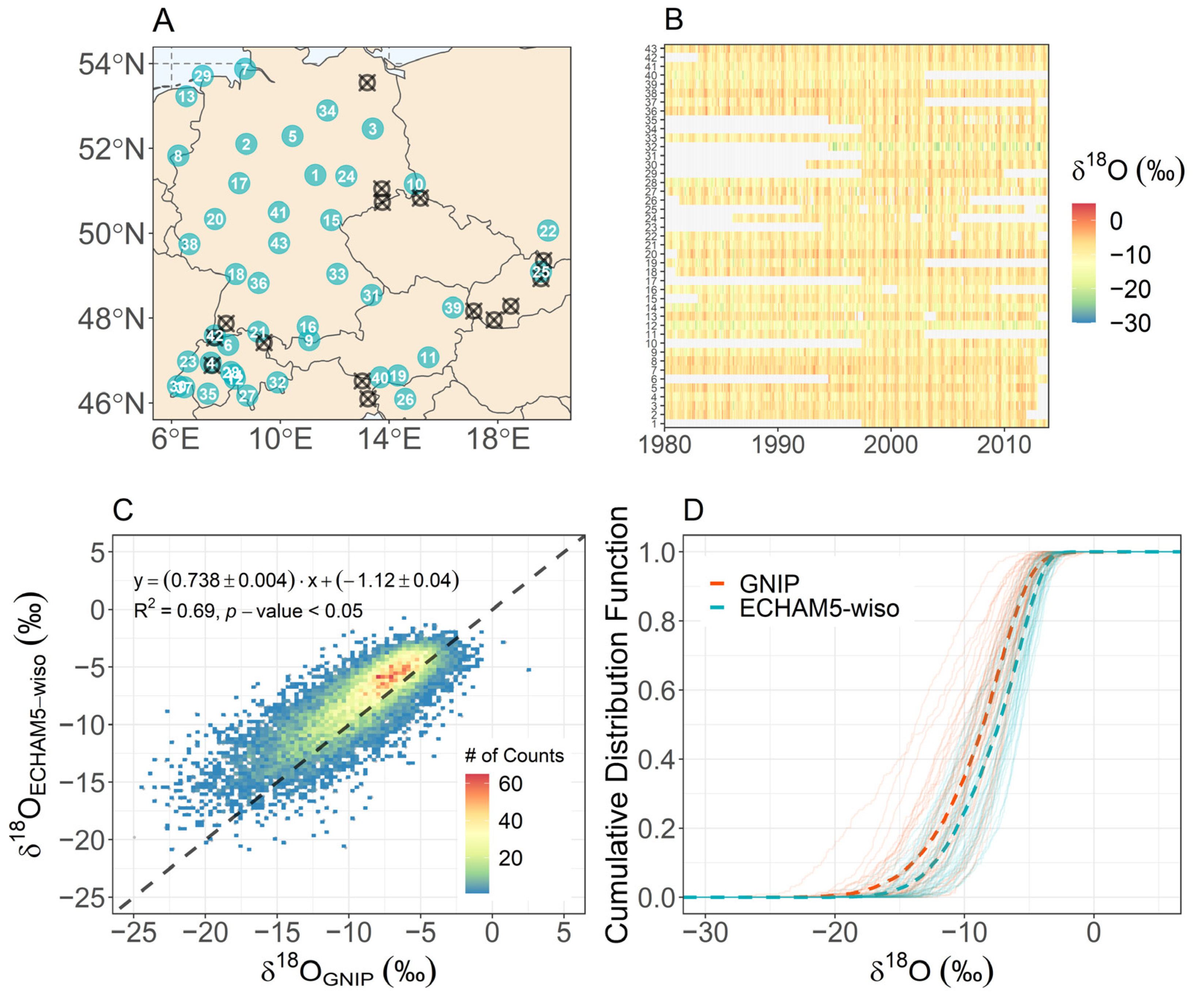
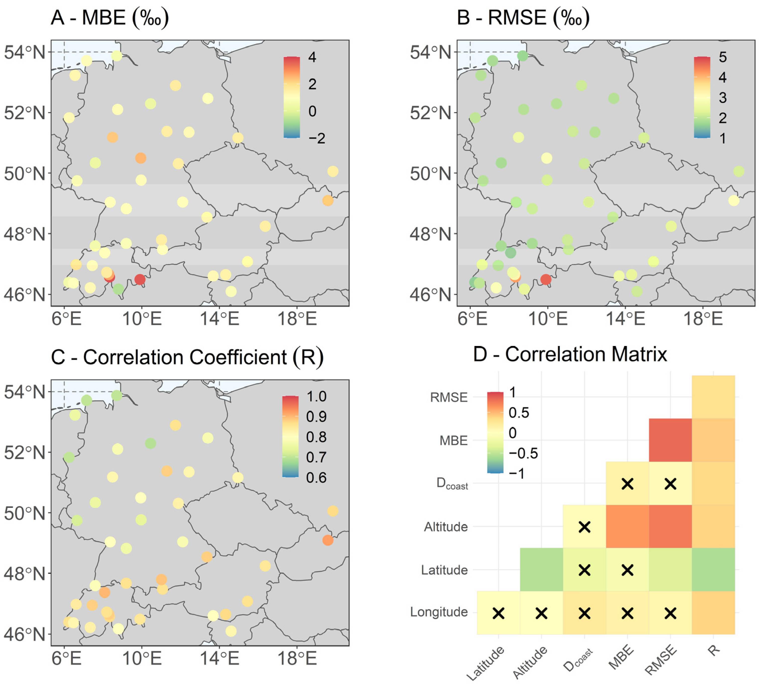
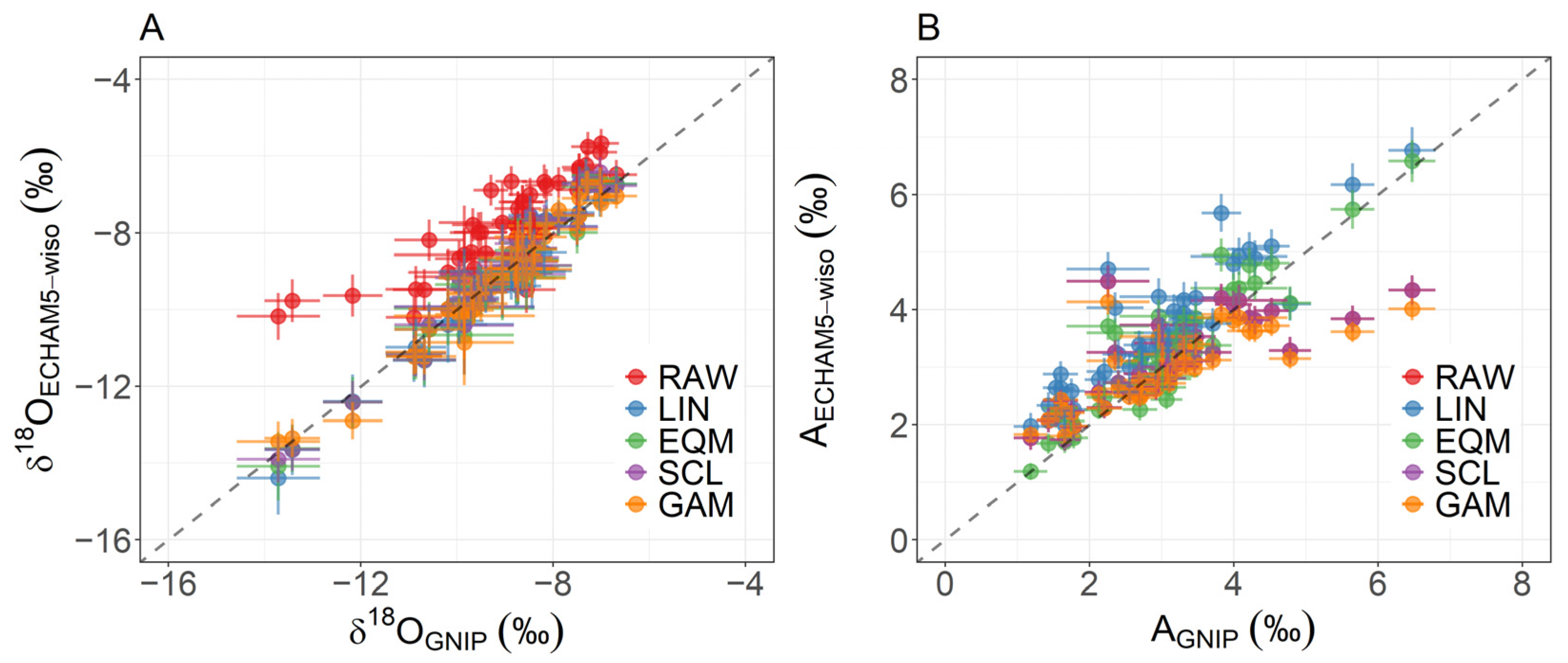
4.1. Validation of δ18OECHAM5-wiso over Central Europe

The temporal distribution of δ18O in precipitation from January 1980 to December 2013 is shown Figure 2A–C. The isotopic composition of precipitation varies seasonally at all sampling sites. The time series of δ18OGNIP and δ18OECHAM5-wiso are temporally consistent following a sinusoidal pattern, also depicting similar maxima (less depleted) locations in summer (Figure 2A,B). This is only to be expected because of the ‘isotope–temperature effect’. More specifically, the isotopic composition of precipitation at middle and high-latitude continental areas shows a strong relationship with air temperature, following the air-temperature sinusoidal pattern across the year. δ18OECHAM-wiso is less depleted than δ18OGNIP with a lower variability. Figure 2C shows the time series of isotopic biases (Δδ18O = δ18OGNIP − δ18OECHAM5-WISO). Δ18O are mainly distributed between −5‰ and 5‰ without revealing a distinct seasonal pattern.
In order to explain in detail the seasonality of δ18O in precipitation, monthly distribution isotopic plots are created in the right panels of Figure 2. The “seasonal effect” is verified with less depleted isotopic signatures in summer for ECHAM5-wiso and GNIP (Figure 2D,E). The tails of the statistical distributions (Figure 2D) include a higher number of measurements in all months for GNIP compared to ECHAM5-wiso. On the other side, the monthly distributions of δ18O are less platykurtic for ECHAM5-wiso in the summer months, indicating the substantial presence of isotopic data across its monthly mean. Regarding Figure 2F, the monthly distributions of isotopic biases are significantly displaced from zero. The distribution’s shape is almost symmetric, with skewness values ranging from −0.35 to 0.17; the differences between the mean and median for the monthly biases slightly differ, extending from −0.14‰ to 0.04‰.
The statistical verification of δ18OECHAM5-wiso against δ18OGNIP is performed in terms of MBE, RMSE, and R. Figure 3A–C shows the spatial distribution of statistical scores for the GNIP sampling sites. In general, δ18OECHAM5-wiso overestimates the observed δ18O in precipitation with positive MBEs in 42 out of 43 stations. The systematic bias ranges from −0.7‰ (Locarno, Switzerland—#27) to 3.8‰ (Grimsel, Switzerland—#12), with an average of 1.3‰. MBE does not show a significant zonal or meridional variation, while the distance from the nearest coastline (Dcoast) does not contribute to the MBE’s spatial pattern (Figure 3A). Figure 3D represents the Pearson’s correlation matrix between the statistical indicators and simple geographical and topographical parameters with significant correlations (p-value < 0.5) for the non-crossed boxes. The pairwise correlations between MBE and Longitude, Latitude, and Dcoast are not significant under the 95% confidence level (p-value > 0.05), implying that the ‘latitude’ and ‘continental’ isotopic effects are not imprinted in the MBE variability. On the other side, elevation is significantly related to MBE, with a correlation coefficient R = 0.67 (p-value ≈ 0). Figure S1A (blue points) shows the MBE–Altitude relationship. The MBE lapse rate equals 1‰/km, with two ‘extreme’ cases in Grimsel (#12) and Pontresina (#32) located in the Swiss Alps at elevations of 1750 m and 1950 m, respectively. ECHAM5-wiso suffers from accurately reproducing the strongly depleted isotopic signatures of precipitation in alpine regions, giving less depleted isotopic signatures and a significantly positive MBE. The substantial overestimation from ECHAM5-wiso relies on the non-accurate resolving of the complex topographic relief such as alpine mountain ridges and slopes due to the coarse spatial resolution [22], resulting in an erroneous representation of the associated isotope fractionation phenomena.
Regarding the dispersion error (RMSE), it ranges between 1.6‰ (Buchs/Suhr, Switzerland—#6) and 4.7‰ (Pontresina, Switzerland—#32), with an average RMSE equal to 2.3‰. Slight spatial RMSE variation can be observed where the site-specific dispersion errors are mostly distributed close to the areal average of 2.3‰. According to the correlation matrix of Figure 3D, RMSE is inversely related to latitude and positively related to elevation. However, the spatial distribution of RMSE (Figure 3B) cannot verify this latitudinal dependency. The scatter plot of Figure S1B represents the relationship between RMSE and latitude. It is distinguishable that stations with RMSE > 3‰ form a distinct cluster, and it probably leads to the significant calculated negative correlation (R = −0.37, p-value = 0.01) of Figure 3D. This cluster includes three Swiss stations: Grimsel—#12, Guttannen—#14, Pontresina—#32, with elevations exceeding 1000 m. By removing these stations, the correlation coefficient is not significant (R = −0.27, p-value = 0.09). Following MBE, the ‘altitude effect’ is also remarkable for RMSE (R = 0.75, p-value ≈ 0), with a lapse rate of ~1‰/km (Figure S1A—red points).
The overestimation of the isotopic signal and the existence of dispersion error in ECHAM5-wiso, due to the incapacity of correctly resolving the complex orography of mountaineous areas, could be partially reduced by using the new version of ECHAM-wiso model (ECHAM6-wiso) [33]. This version is characterized by a higher spatial resolution (~0.9° × 0.9°) and uses the ERA5 reanalysis instead of the ERA-Interim data. However, the comparison of the two ECHAM-wiso versions and the application of bias correction methods on the isotopic products is beyond the scope of this paper and could be addressed in the future.
Finally, ECHAM5-wiso model and GNIP are compared in terms of the Pearson’s R correlation coefficient. δ18OECHAM5-wiso shows good agreement against δ18OGNIP with R ranging between 0.69 (Braunschweig, Germany—#3) and 0.92 (Liptovsky-Mikulas Ondrasova, Slovakia—#25). All calculated R values are significant under the 95% confidence level. In contrast to MBE and RMSE, R represents remarkable ‘latitude’, ‘continentality’, and ‘altitude’ isotopic effects. (Figure 3D). According to the spatial map (Figure 3C) and the scatterplots (Figure S1D,E), a slightly significant positive change of R is depicted for more continental regions (p-value = 0.01 for R vs. Longitude and p-value = 0.02 for R vs. Dcoast). The correlation coefficient decreases for higher latitudes, revealing a remarkable latitudinal change (Figure S1C). Finally, a non-linear pattern is extracted between R and Altitude, with positive changes for Altitude < 500 m and a neutral pattern for higher elevations (Figure S1F).

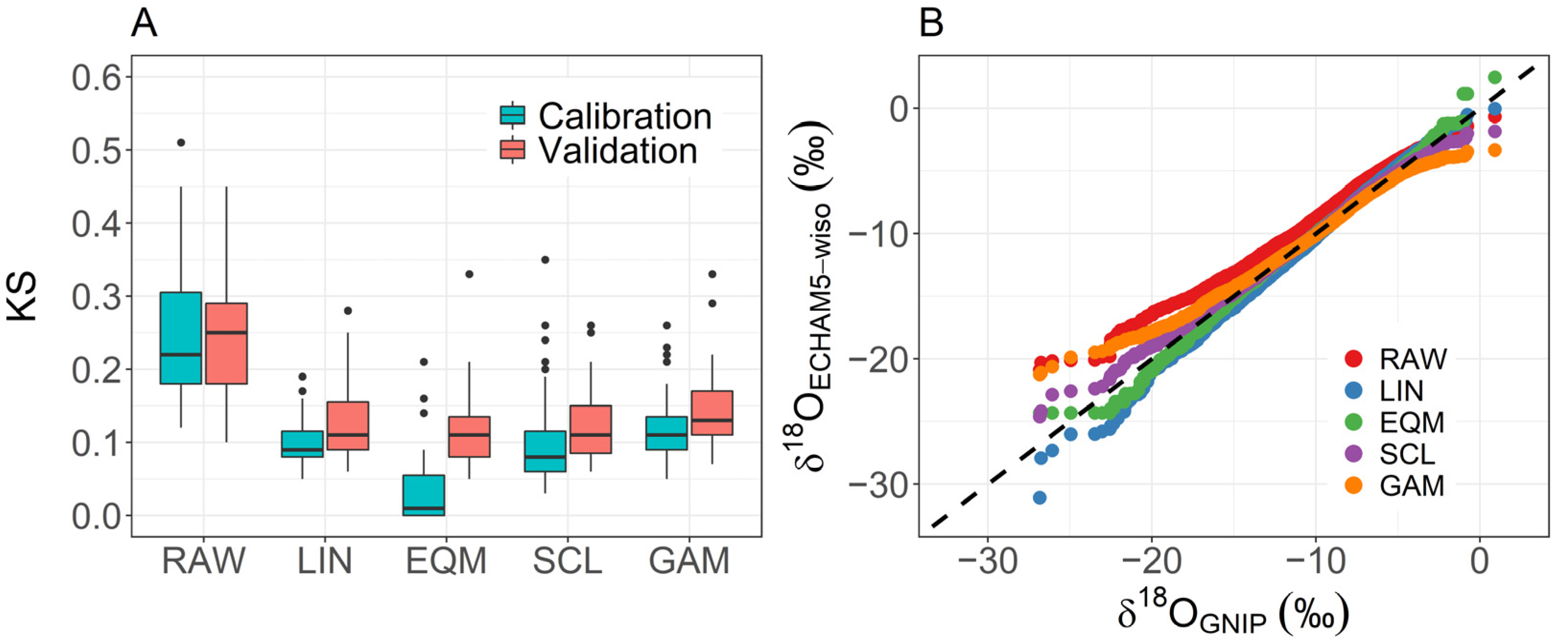
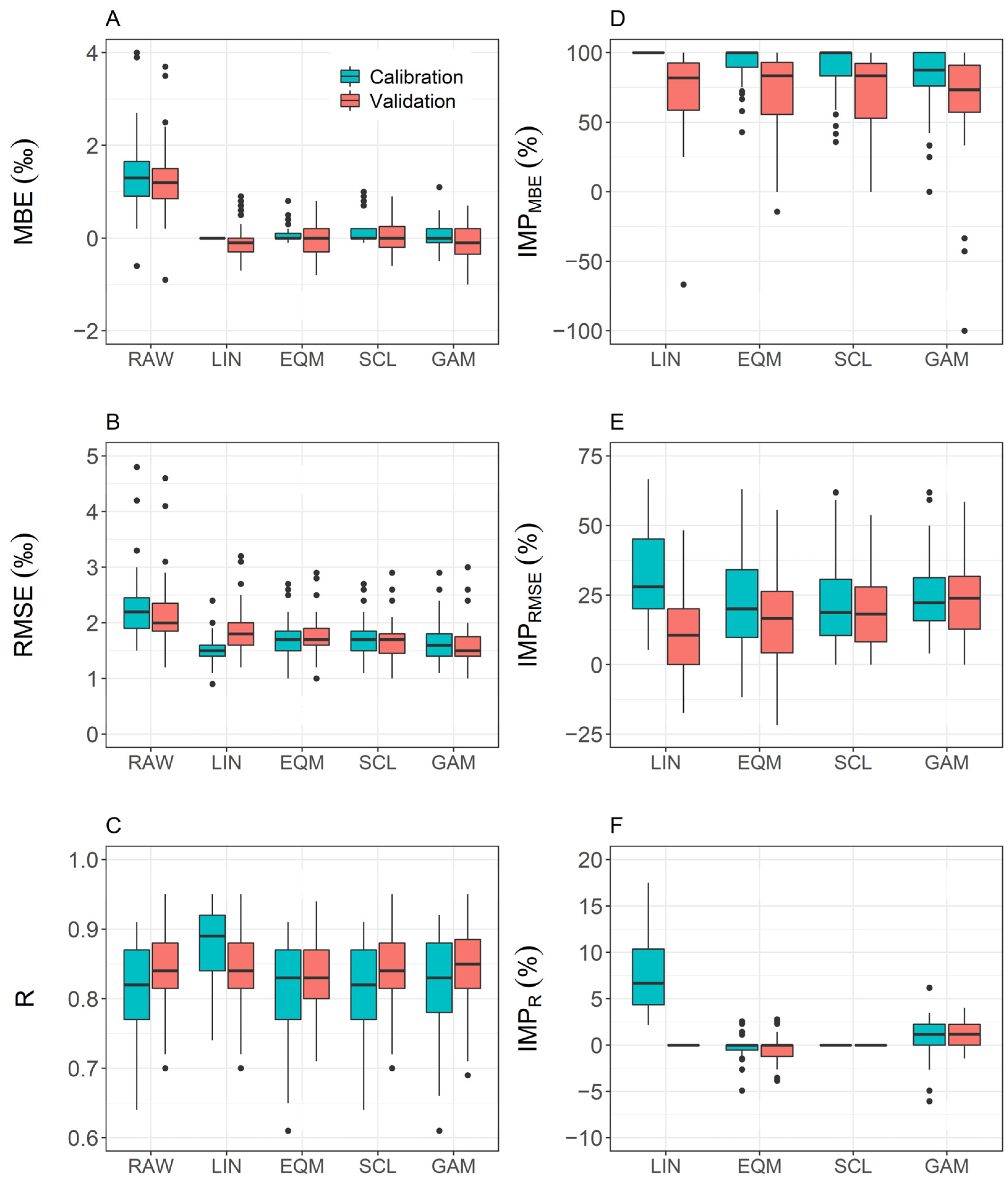
4.2. Bias Correction of δ18OECHAM5-wiso

The existence of systematic and dispersion errors between δ18OECHAM5-wiso and δ18OGNIP demonstrates the necessity of evaluating bias correction techniques. In this study, four different algorithms are applied (“Methods”—Section 3), namely Linear Bias Removal (LIN), Empirical Quantile Mapping (EQM), Linear Scaling (SCL), and Generalized Additive Models (GAMs). RAW denotes the uncorrected or initial δ18OECHAM5-wiso. As already discussed in the “Methods” section, the bias correction techniques are firstly designed using isotopic and auxiliary measurements (geographic and topographic parameters) of the calibration period (January 1980–December 2000), and the evaluation against observations of the validation period (January 2001–December 2013) is performed in terms of MBE, RMSE, and R statistical scores.
In general, the performance and the error patterns are substantially improved using the bias-corrected isotopic composition. Regarding MBE (Figure 4A), all methods perform efficiently with medians (thick black line inside each box) close to zero and minimal variability, implying the substantial reduction in systematic biases using corrected isotopic products. It is worth mentioning that LIN adjusts δ18OECHAM5-wiso along the 1:1 line; therefore, it is normal to eliminate the systematic bias during calibration. The MBE improvement, IMPMBE (Figure 4D), for the validation period is above 70%, with higher values approaching 85% for LIN, EQM, and SCL and also high improvements for all bias correction algorithms (IMPMBE > 90%) during calibration.
According to Figure 4B, the corrected δ18OECHAM5-wiso exhibit reduced dispersion errors. The median (1.6‰) and the individual quantiles of RMSE are lower for GAMs compared to the other bias correction methods (Figure 4B) for the validation period. IMPRMSE lies within 0–53.4% and 0–58.5% with median values of 19.9% and 23.5% for SCL and GAM, respectively (Figure 4E). LIN works efficiently only in the calibration period and IMPRMSE extends between 5.43% and 66.7%, with a median value of 28%. However, a similar pattern is not extracted for the validation period, and LIN shows the worst performance in terms of RMSE (1.2–3.2‰; median = 1.9‰) and IMPRMSE (−17.4–48.3%; median = 10.6%). Similar but slightly improved metrics are shown for EQM compared to LIN, with RMSE: 1–2.9‰; median = 1.8‰ and IMPRMSE: −21.4–55.6‰; median = 16.4‰. LIN and EQM also provide negative IMPRMSE at 10 and 3 sampling sites, respectively.
Finally, the correlation coefficient (R) and its improvement metric (IMPR) examine the overall performance of bias-corrected isotopic data. R is high for the RAW and the bias-corrected δ18OECHAM5-wiso in both calibration and validation periods. EQM, SCL, and GAMs show similar R patterns with higher R values for LIN during calibration; IMPR ranges from 2.5% to 17.5%. However, the R for the validation period indicates that the GAM provides better results than the other methods. Additionally, the boxplots for R and IMPR regarding the validation period for LIN and SCL result in a non-significant change in the correlation coefficient, as expected by the algorithmic structure of the bias correction techniques (“Methods”—Section 3).
The statistical evaluation of the bias-corrected δ18OECHAM5-wiso is also performed in a monthly basis by grouping the statistical scores for each calendar month. EQM, SCL, and GAMs show better MBE and RMSE patterns compared to LIN, as obtained by the monthly whiskers in Figure 5A,B. The MBE boxplots for LIN from November to March include mainly negative systematic biases, implying an underestimation of GNIP isotopic observations and more depleted isotopic signatures for LIN. Moreover, RMSE for LIN is higher than the other bias correction algorithms for those months. The promising outcomes from Figure 5A,B are (a) the substantial reduction in systematic biases from bias-corrected δ18OECHAM5-wiso, and (b) the dispersion error is reduced for all calendar months. Figure 5C displays the monthly boxplots for the correlation coefficient, R, with a higher correlation from August to March. However, the differences in the boxplot shapes between RAW and the bias-corrected isotopic composition are not distinguishable.
Another critical aspect is to investigate how bias correction algorithms improve the statistical similitude between the modelled and the observed parameter. Apart from the error and the overall performance metrics, bias correction techniques aim to adjust the modelled statistical distributions to follow those of observations. As already reported in the ‘Data Sources’ section and in Figure 1D, the statistical distributions of δ18OGNIP and δ18OECHAM5-wiso significantly differ according to the Kolmogorov–Smirnov statistical test (KS-test).
The bias-corrected products provide lower KS values compared to the RAW δ18OECHAM5-wiso (Figure 6A). EQM optimally projects the modelled statistical distribution to follow the observed ones as presented by the KS boxplots (Figure 6A) and the Quantile–Quantile (Q-Q) graph (Figure 6B). The EQM quantiles are close to the observed, with differences mainly in the tails of the observed distribution. SCL behaves similarly with EQM, though with higher deviations from observed quantiles, especially in the lower tail. For δ18OGNIP < −20‰, the GAM overestimates and LIN underestimates the observed quantiles, while, for δ18OGNIP > −5‰, the GAM shows the highest underestimation.

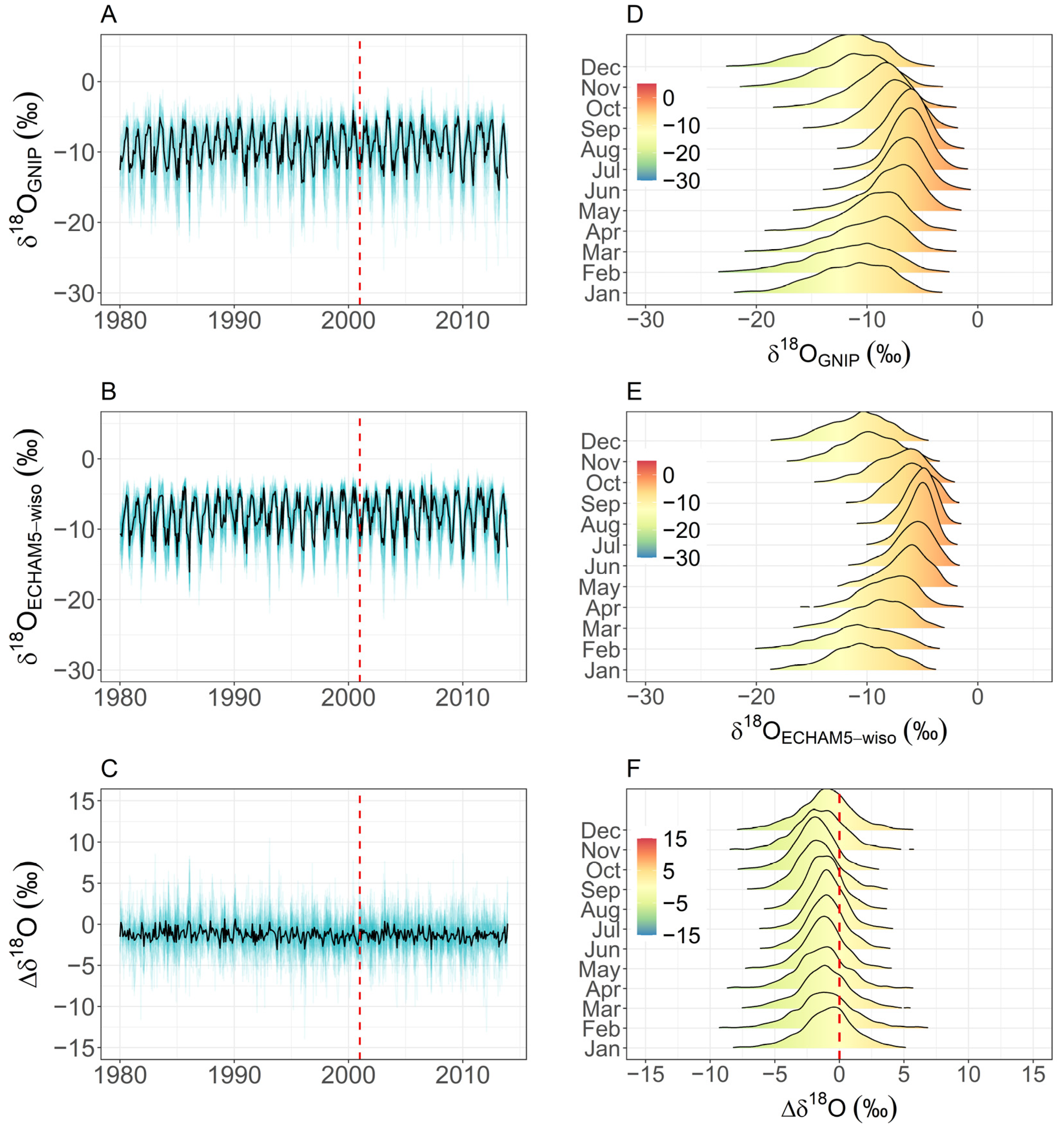
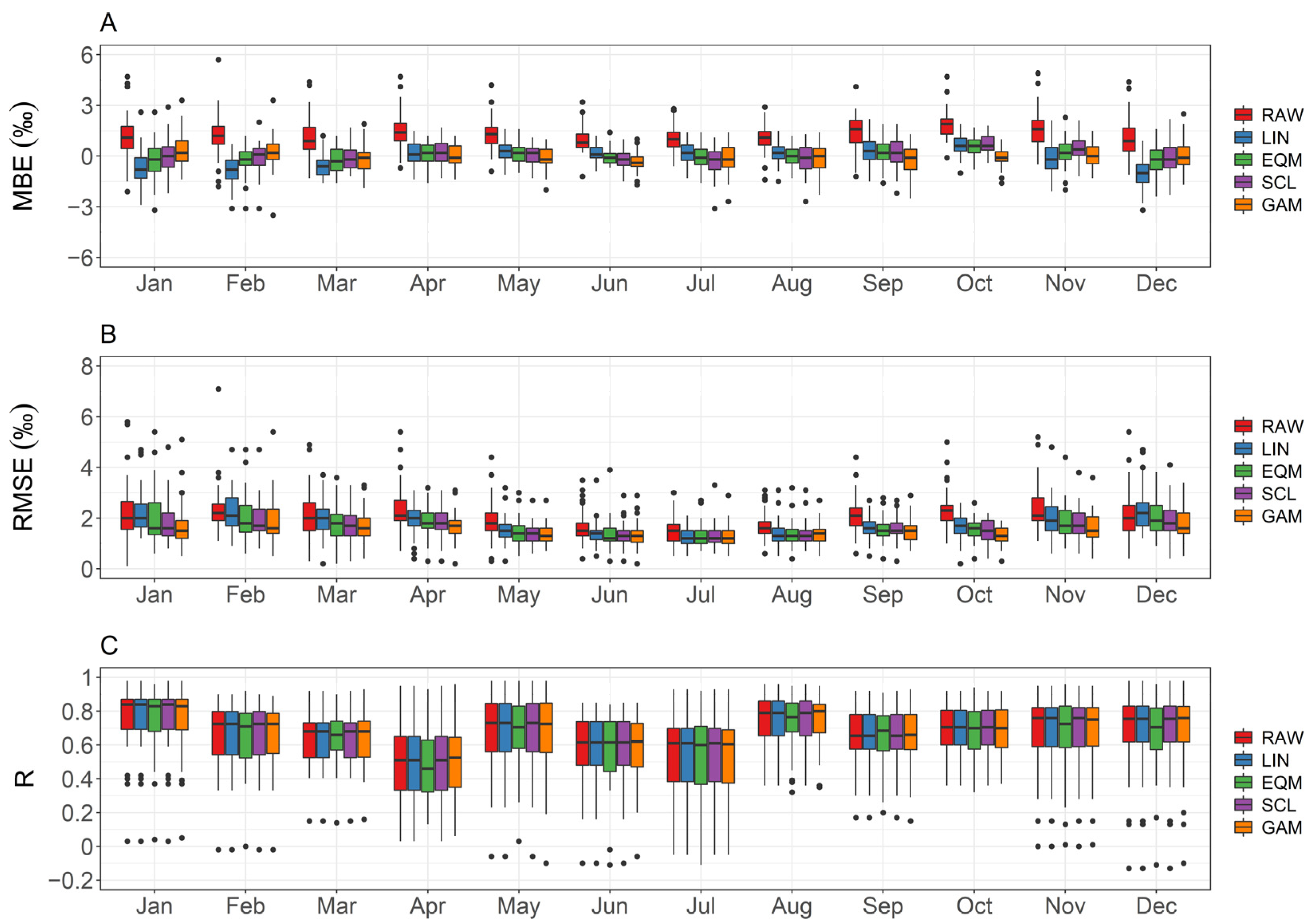
4.3. Long-Term Performance and Seasonal Amplitude of Bias-Corrected δ18OECHAM5-wiso

The long-term performance is assessed by comparing the climatology between the RAW and the bias-corrected δ18OECHAM5-wiso against GNIP observations over the validation period. Long-term monthly means and the corresponding 95% uncertainty ranges are calculated for each station separately. The initially modelled δ18OECHAM5-wiso data are less depleted compared to observations providing a positive mean bias of 1.3‰ and a dispersion error of 1.5‰ (Figure 7A). The long-term δ18OECHAM5-wiso data extends from −13.7‰ to −6.68‰, with a median of approximately −9‰. Similar ranges and medians are depicted for the bias correction methods, with a less depleted median value by ~2‰ for RAW. Bias-corrected δ18OECHAM5-wiso data are in excellent agreement with δ18OGNIP with R = 0.98, the systematic bias is completely eliminated, and the dispersion biases are very low (RMSE < 0.38‰). Another significant point, especially for hydrological or climatological applications that require information about the long-term isotopic value of precipitation, is to examine the displacement of the long-term simulated means from the identical line (1:1). Bias correction techniques adjust the long-term isotopic means to follow the observations, providing a slight displacement from the 1:1 (~1%) with the relevant linear slope for RAW to reach 0.68. The long-term isotopic composition is substantially corrected in high-altitude alpine sampling sites (Grimsel—#12, Pontresina—#14 and Guttannen—#32) with δ18OGNIP < −12‰. The absolute differences between the RAW δ18OECHAM5-wiso and δ18OGNIP are higher than 3‰, and, after bias correction, the differences drop to ~0.5‰.
The stable isotopic composition of precipitation varies periodically, and it follows a distinct seasonal pattern, being more remarkable in continental and non-equatorial regions [34]. The examination of the seasonal amplitude of δ18O in precipitation is emphasized due to its contribution to climatic studies and estimating the age of young streamflow water and plant water sources [35,36]. Based on [34,35,36,37], the isotopic amplitude of the sampling sites can be modelled using sinusoidal curves. Here, the amplitudes are calculated for RAW and bias-corrected δ18OECHAM5-wiso of the validation period and then compared against GNIP observations. The scatter plots of Figure 7B show the results, where the error bars correspond to ±1 × SE of calculated amplitudes. The isotopic amplitude for GNIP ranges from 1.2‰ to 6.5‰, with higher values for more inland stations due to the less pronounced maritime responses and more remarkable seasonal fluctuation in air temperature. For more information about the geographical and topographical responses of isotopic amplitude in Central Europe, refer to [37].
RAW and SCL have identical amplitudes ranging from 1.7‰ to 4.5‰, since SCL corrects the modelled δ18OECHAM5-wiso by the systematic bias adjustment. The slope of the best fit line and the correlation coefficient are calculated equal to 0.5 and 0.78. GAM produces similar results to RAW and SCL, and it fails to accurately reproduce the GNIP amplitude, especially for values higher than 4‰. According to Figure 7B, EQM shows the best results with an amplitude range (1.2‰ to 6.6‰), exhibiting a small displacement by the 1:1 line (the slope of the best fit line is 0.93) and good agreement (R = 0.92) with GNIP-observed amplitudes.

5. Conclusions

The isotope-enabled General Circulation Models simulate the spatiotemporal patterns of the δ18O values of precipitation by incorporating isotope physics into the equations describing the individual components of the atmospheric water cycle. Although iGCMs predict with relevant accuracy the precipitation δ18O distribution at regional and global scales, the inaccurate representation of the isotopic fractionation phenomena during various atmospheric processes as well as the inability to reproduce the observed δ18O in areas with complex topographic settings induce several biases into the isotopic outputs. The application of bias correction methodologies aims to adjust the model inconsistencies by reducing the systematic and dispersion biases compared to observations.
In this study, δ18O in precipitation from the ECHAM5-wiso GCM model is validated against GNIP observations in Central Europe over a period extending from January 1980 to December 2013. The intercomparison results show that the ranges of MBE, RMSE, and R are from −0.7‰ to 3.8‰, 1.6‰ to 4.7‰, and 0.69 to 0.92, respectively. Higher systematic and dispersion errors exist in high latitude alpine sites since ECHAM5-wiso fails to capture the isotopic variability in regions with complex topographic relief, mainly because of its coarse model’s spatial resolution. The statistical scores are strongly related to elevation, with a p-value << 0.05, while ‘latitudinal’ and ‘continental’ responses are remarkable only for the correlation coefficient. In order to improve the δ18OECHAM5-wiso simulations, four bias correction algorithms (LIN, EQM, SCL, and GAM) are employed to reduce the possible systematic and dispersion errors. MBE is substantially reduced using the bias-corrected δ18OECHAM5-wiso, with IMPMBE exceeding 70%. Reduced RMSEs are calculated for the corrected δ18OECHAM5-wiso and show median improvements for SCL and GAM methods higher than 20%. LIN and EQM show similar ranges and medians for RMSE and IMPRMSE. The bias-corrected δ18OECHAM5-wiso are compared against δ18OECHAM5-wiso in terms of the overall performance. However, the correlation coefficient is not substantially improved. Regarding the statistical similitude, δ18OECHAM5-wiso follows observations with EQM to provide similar quantiles with the observed ones. Bias correction techniques adjust the long-term modelled isotopic means to follow the observations correcting the initial displacement from the 1:1 line. Promising results are derived for the high-altitude alpine sites, where the differences among the modelled and the observed δ18O drop to 0.5‰ (from 3‰) after applying bias correction. Finally, the isotopic amplitude for describing the seasonal variation of precipitation isotopes is calculated using sinusoidal models for the observed, the initial modelled, and the bias-corrected δ18O. GAM, SCL, and LIN methods produce accurate isotopic amplitudes for observed cases lower than 4‰, while EQM reproduces the GNIP amplitudes successfully both in range and magnitude.
A follow-up of this study would be to examine how bias correction methods modulate the ‘temperature’ and ‘rainfall amount’ effects over various regions in the globe. A possible application in areas with complex climates could be beneficial in assessing and improving the performance of iGCMs. The spatiotemporal extension of the bias correction procedure is planned to derive contiguousness both in time and space bias-corrected δ18OECHAM5-wiso data instead of using station-wise-corrected isotopic time series.

Supplementary Materials

The following supporting information can be downloaded at: https://www.mdpi.com/article/10.3390/oxygen2020010/s1, Table S1: Details of the GNIP sampling sites used in this study; Figure S1: Statistical scores (MBE, RMSE, and R) against geographical and topographical parameters.

Author Contributions

Conceptualization, V.S. and A.A.A.; methodology, V.S.; validation, A.A.A.; data curation, V.S.; writing—original draft preparation, V.S.; writing—review and editing, A.A.A.; supervision, A.A.A. All authors have read and agreed to the published version of the manuscript.

Funding

This research received no external funding.

Institutional Review Board Statement

Not applicable.

Informed Consent Statement

Not applicable.

Data Availability Statement

Data used in this study can be found in: https://doi.org/10.1594/PANGAEA.902347 (ECHAM5-wiso) and https://nucleus.iaea.org/wiser (GNIP), accessed on 14 March 2022.

Acknowledgments

The authors would like to acknowledge the International Atomic Energy Agency (IAEA) for the ongoing maintenance of the Global Network of Isotopes in Precipitation (GNIP) and the provision of isotopic datasets.

Conflicts of Interest

The authors declare no conflict of interest.

References

  1. Bigeleisen, J. Chemistry of isotopes. Science 1965, 147, 463–471. [Google Scholar] [CrossRef] [PubMed]
  2. Dansgaard, W. Stable isotopes in precipitation. Tellus 1964, 16, 436–468. [Google Scholar] [CrossRef]
  3. Gat, J.R. Oxygen and hydrogen isotopes in the hydrologic cycle. Ann. Rev. Earth Planet. Sci. 1996, 24, 225–262. [Google Scholar] [CrossRef] [Green Version]
  4. IAEA/WMO. Global Network of Isotopes in Precipitation. The GNIP Database. Available online: https://nucleus.iaea.org/wiser (accessed on 1 February 2022).
  5. Hoffmann, G.; Werner, M.; Heimann, M. Water isotope module of the ECHAM atmospheric general circulation model: A study on timescales from days to several years. J. Geophys. Res. 1998, 103, 16871–16896. [Google Scholar] [CrossRef] [Green Version]
  6. Schmidt, G.; LeGrande, A.; Hoffmann, G. Water isotope expressions of intrinsic and forced variability in a coupled ocean-atmosphere model. J. Geophys. Res. 2007, 112, D10103. [Google Scholar] [CrossRef]
  7. Lee, J.-E.; Fung, I.; DePaolo, D.; Fennig, C.C. Analysis of the global distribution of water isotopes using the NCAR atmospheric general circulation model. J. Geophys. Res. 2007, 112, D16306. [Google Scholar] [CrossRef]
  8. Yoshimura, K.; Kanamitsu, M.; Noone, D.; Oki, T. Historical isotope simulation using reanalysis atmospheric data. J. Geophys. Res. 2008, 113, D19108. [Google Scholar] [CrossRef]
  9. Risi, C.; Bony, S.; Vimeux, F.; Jouzel, J. Water stable isotopes in the LMDZ4 general circulation model: Model evaluation for present day and past climates and applications to climatic interpretations of tropical isotopic records. J. Geophys. Res. 2010, 115, D12118. [Google Scholar] [CrossRef] [Green Version]
  10. Tindall, J.C.; Valdes, P.J.; Sime, L.C. Stable water isotopes in HadCM3: Isotopic signature of El Nino Southern Oscillation and the tropical amount effect. J. Geophys. Res. 2009, 114, D04111. [Google Scholar] [CrossRef] [Green Version]
  11. Werner, M.; Langebroek, P.M.; Carlsen, T.; Herold, M.; Lohmann, G. Stable water isotopes in the ECHAM5 general circulation model: Toward high-resolution isotope modeling on a global scale. J. Geophys. Res. 2011, 116, 15109. [Google Scholar] [CrossRef]
  12. Kurita, K.; Noone, D.; Risi, C.; Schmidt, G.A.; Yamada, H.; Yoneyama, K. Intraseasonal isotopic variation associated with the Madden-Julian Oscillation. J. Geophys. Res. 2011, 116, D24101. [Google Scholar] [CrossRef]
  13. Dee, S.; Noone, D.D.; Buenning, N.; Emile-Geay, J.; Zhou, Y. SPEEDY-IER: A fast atmospheric GCM with water isotope physics. J. Geophys. Res. Atmos. 2015, 120, 73–91. [Google Scholar] [CrossRef]
  14. Sturm, K.; Hoffmann, G.; Langmann, B.; Stichler, W. Simulation of delta O-18 in precipitation by the regional circulation model REMOiso. Hydrol. Processes 2005, 19, 3425–3444. [Google Scholar] [CrossRef]
  15. Pfahl, S.; Wernli, H.; Yoshimura, K. The isotopic composition of precipitation from a winter storm—A case study with the limited-area model COSMOiso. Atmos. Chem. Phys. 2012, 12, 1629–1648. [Google Scholar] [CrossRef] [Green Version]
  16. Delavau, C.J.; Stadnyk, T.; Holmes, T. Examining the impacts of precipitation isotope input (δ18Oppt) on distributed, tracer-aided hydrological modelling. Hydrol. Earth Syst. Sci. 2017, 21, 2595–2614. [Google Scholar] [CrossRef] [Green Version]
  17. Peng, P.; Zhang, X.J.; Chen, J. Bias correcting isotope-equipped GCMs outputs to build precipitation oxygen isoscape for Eastern China. J. Hydrol. 2020, 589, 125153. [Google Scholar] [CrossRef]
  18. Nan, Y.; He, Z.; Tian, F.; Wei, Z.; Tian, L. Can we use precipitation isotope outputs of isotopic general circulation models to improve hydrological modeling in large mountainous catchments on the Tibetan Plateau? Hydrol. Earth Syst. Sci. 2021, 25, 6151–6172. [Google Scholar] [CrossRef]
  19. Kottek, M.; Grieser, J.; Beck, C.; Rudolf, B.; Rubel, F. World Map of the Köppen-Geiger climate classification updated. Meteorol. Z. 2006, 15, 259–263. [Google Scholar] [CrossRef]
  20. Werner, M. ECHAM5-wiso simulation data-present-day, mid-Holocene, and Last Glacial Maximum. PANGAEA. Available online: https://doi.org/10.1594/PANGAEA.902347 (accessed on 1 February 2022). [CrossRef]
  21. Butzin, M.; Werner, M.; Masson-Delmotte, V.; Risi, C.; Frankenberg, C.; Gribanov, K.; Jouzel, J.; Zakharov, V.I. Variations of oxygen-18 in West Siberian precipitation during the last 50 years. Atmos. Chem. Phys. 2014, 14, 5853–5869. [Google Scholar] [CrossRef] [Green Version]
  22. Langebroek, P.M.; Werner, M.; Lohmann, G. Climate information imprinted in oxygen-isotopic composition of precipitation in Europe. Earth Planet. Sci. Lett. 2016, 311, 144–154. [Google Scholar] [CrossRef]
  23. Polo, J.; Fernández-Peruchena, C.M.; Salamalikis, V.; Mazorra-Aguiar, L.; Turpin, M.; Martín-Pomares, L.; Kazantzidis, A.; Blanc, P.; Remund, J. Benchmarking on improvement and site-adaptation techniques for modeled solar radiation datasets. Solar Energy 2020, 201, 469–479. [Google Scholar] [CrossRef]
  24. Gudmundsson, L.; Bremnes, J.; Haugen, J.; Engen-Skaugen, T. Technical note: Downscaling RCM precipitation to the station scale using statistical transformations—A comparison of methods. Hydrol. Earth Syst. Sci. 2012, 16, 3383–3390. [Google Scholar] [CrossRef] [Green Version]
  25. Themeßl, M.J.; Gobiet, A.; Heinrich, G. Empirical-statistical downscaling and error correction of regional climate models and its impact on the climate change signal. Clim. Chang. 2012, 112, 449–468. [Google Scholar] [CrossRef]
  26. Piani, C.; Weedon, G.P.; Best, M.; Gomes, S.M.; Viterbo, P.; Hagemann, S.; Haerter, J.O. Statistical bias correction of global simulated daily precipitation and temperature for the application of hydrological models. J. Hydrol. 2010, 395, 199–215. [Google Scholar] [CrossRef]
  27. Teutschbein, C.; Seibert, J. Bias correction of regional climate model simulations for hydrological climate-change impact studies: Review and evaluation of different methods. J. Hydrol. 2012, 456–457, 12–29. [Google Scholar] [CrossRef]
  28. Vrac, M.; Marbaix, P.; Paillard, D.; Naveau, P. Non-linear statistical downscaling of present and LGM precipitation and temperatures over Europe. Clim. Past 2007, 3, 669–682. [Google Scholar] [CrossRef] [Green Version]
  29. Latombe, G.; Burke, A.; Vrac, M.; Levavasseur, G.; Dumas, C.; Kageyama, M.; Ramstein, G. Comparison of spatial downscaling methods of general circulation model results to study climate variability during the Last Glacial Maximum. Geosci. Model Dev. 2018, 11, 2563–2579. [Google Scholar] [CrossRef] [Green Version]
  30. Beyer, R.; Krapp, M.; Manica, A. An empirical evaluation of bias correction methods for palaeoclimate simulations. Clim. Past 2020, 16, 1493–1508. [Google Scholar] [CrossRef]
  31. Hastie, T.J.; Tibshirani, R.J. Generalized Additive Models; Chapman and Hall: London, UK, 1990. [Google Scholar]
  32. Wood, S.N. Fast stable restricted maximum likelihood and marginal likelihood estimation of semiparametric generalized linear models. J. R. Stat. Soc. B 2011, 73, 3–36. [Google Scholar] [CrossRef] [Green Version]
  33. Cauquoin, A.; Werner, M. High-resolution nudged isotope modeling with ECHAM6-wiso: Impacts of updated model physics and ERA5 reanalysis data. J. Adv. Model. Earth Syst. 2021, 13, e2021MS002532. [Google Scholar] [CrossRef]
  34. Feng, X.; Faiia, A.M.; Posmentier, E.S. Seasonality of isotopes in precipitation: A global perspective. J. Geophys. Res. 2009, 114, D08116. [Google Scholar] [CrossRef] [Green Version]
  35. Allen, S.T.; Jasechko, S.; Berghuijs, W.R.; Welker, J.M.; Goldsmith, G.R.; Kirchner, J.W. Global sinusoidal seasonality in precipitation isotopes. Hydrol. Earth Syst. Sci. 2019, 23, 3423–3436. [Google Scholar] [CrossRef] [Green Version]
  36. Kirchner, J.W. Aggregation in environmental systems–Part 1: Seasonal tracer cycles quantify young water fractions, but not mean transit times, in spatially heterogeneous catchments. Hydrol. Earth Syst. Sci. 2016, 20, 279–297. [Google Scholar] [CrossRef] [Green Version]
  37. Salamalikis, V.; Argiriou, A.A.; Dotsika, E. Periodicity analysis of δ18O in precipitation over Central Europe: Time–frequency considerations of the isotopic ‘temperature’ effect. J. Hydrol. 2016, 534, 150–163. [Google Scholar] [CrossRef]
Figure 1. (A) Spatial distribution of GNIP isotope sampling sites ranked in alphabetical order (Table S1). The colored circles superimposed with station index are used for further analysis. The circle symbols with superimposed crosses indicate the sampling sites without available measurements into January 1980–December 2010 (training period) or January 2001–December 2013 (testing period); (B) heatmap of δ18O data availability for each sampling site from January 1980 to December 2013. The blank cells correspond to missing δ18O data. (C) Scatter density plot between δ18O from GNIP (δ18OGNIP) and δ18O from ECHAM5-wiso model (δ18OECHAM5-wiso). (D) Cumulative Distribution Functions (CDF) for δ18OGNIP (red lines) and δ18OECHAM5-wiso (blue lines). The solid lines correspond to site-specific CDFs and the dashed lines correspond to the CDFs using all available isotopic records from GNIP and ECHAM5-wiso model.
Oxygen 02 00010 g001
Figure 2. Time series of (A) δ18OGNIP, (B) δ18OECHAM5-WISO, and (C) Δδ18O = δ18OGNIP − δ18OECHAM5-WISO. The blue lines represent the temporal distribution of δ18O for the central European stations and the solid black line represents the average δ18O for the whole study area. The vertical red line separates the measurement dataset into the calibration (January 1980–December 2000) and validation (January 2001–December 2013) periods. Monthly statistical distributions for (D) δ18OGNIP, (E) δ18OECHAM5-WISO, and (F) Δδ18O = δ18OGNIP − δ18OECHAM5-WISO from January 1980 to December 2013. The plots are generated using all available δ18O measurements for each calendar month. The colored regions within each distribution plot display the δ18O magnitude.
Oxygen 02 00010 g002
Figure 3. Spatial distribution of (A) mean bias error (MBE), (B) Root Mean Square Error (RMSE), and (C) correlation coefficient (R) calculated between δ18OGNIP and δ18OECHAM5-wiso. MBE and RMSE are in ‰. (D) Correlation matrix between the statistical indices (MBE, RMSE, and R) and simple geographical parameters: Latitude, Longitude, Altitude, and Distance from the nearest coastline (Dcoast). The crosses inside the boxes indicate non-significant correlations under the 95% confidence level.
Oxygen 02 00010 g003
Figure 4. Boxplots of statistical scores and improvement indices: (A,D) mean bias error (MBE), (B,E) Root Mean Square Error (RMSE), and (C,F) correlation coefficient (R) using the raw and the bias-corrected δ18OECHAM5-wiso for the calibration (January 1980–December 2000) and the validation (January 2001–December 2013) periods. The thick black lines inside the boxes represent the median value (Q50%) and the black dots correspond to the outliers.
Oxygen 02 00010 g004
Figure 5. Monthly boxplots of (A) mean bias error (MBE), (B) Root Mean Square Error (RMSE), and (C) correlation coefficient (R) of RAW and bias-corrected δ18OECHAM5-wiso for the validation period (January 2001–December 2013). The thick black lines inside the boxes represent the median of the statistical scores and the black dots correspond to the outliers.
Oxygen 02 00010 g005
Figure 6. (A) Boxplots of Kolmogorov–Smirnov (KS) statistic and (B) Quantile–Quantile (Q-Q) plot between δ18OGNIP and the RAW or bias-corrected δ18OECHAM5-wiso for the calibration period (January 1980–December 2000). The thick black lines inside the boxes represent the median value (Q50%) and the black dots correspond to the outliers.
Oxygen 02 00010 g006
Figure 7. (A) δ18OECHAM5-wiso vs. δ18OGNIP. The error bars are ±2 × SE from the calculated average. (B) AECHAM5-wiso vs. AGNIP with A-amplitude calculated using sinusoidal models. The error bars are ±1 × SE from the isotopic amplitude. The dashed black line corresponds to the perfect fit line (1:1).
Oxygen 02 00010 g007
Publisher’s Note: MDPI stays neutral with regard to jurisdictional claims in published maps and institutional affiliations.

