Interaction Between the Longshore Current and the Undertow Induced by the Turbulent Flow in the Surf Zone of Oblique Spilling Breakers

Abstract

The three-dimensional, turbulent, free-surface flow developing in the surf zone over a constant-slope beach as a result of the interaction between the longshore current and the undertow, induced by spilling wave breaking oblique to the shoreline, is numerically simulated. The simulations are performed by implementing the large-wave simulation (LWS) method in a numerical solver of the three-dimensional Navier–Stokes equations. According to the LWS method, large velocity and free-surface elevation scales are fully resolved, while the effect of the corresponding subgrid scales is modeled by eddy-viscosity stresses. The model validation is based on the comparison between the present numerical results and existing experimental measurements for a case of incident regular waves propagating normal to the shoreline over a bed of constant slope 1/35. It is found that the LWS model adequately predicts the wave-breaking parameters—breaking height and depth—and the undertow vertical profiles in the surf zone. Then, two cases of oblique waves, with wave incidence angles of 20° and 30°, and all other parameters identical to those of the validation case, are considered. The numerical results include the gradual breaking process of the refracted waves, as well as the three-dimensional structure of the longshore current and the undertow in the surf zone. In the outer surf zone, the undertow has a larger velocity magnitude than the longshore current, while in the inner surf zone, the opposite occurs.

1. Introduction

The wave-induced currents in the nearshore region are of great interest in coastal engineering due to their impact on sediment transport processes and bed morphodynamics. The generation of these currents is directly connected to wave breaking and dissipation in the surf zone, and they are distinguished into the longshore current, which appears when the direction of wave propagation and breaking is oblique to the shoreline, and the undertow, which has a cross-shore direction. Several theoretical, numerical, and laboratory models have appeared in the literature for each of those currents, and only a brief review is presented here; see Christensen et al. [1] for a detailed review.

The existence of the undertow, which was first described as a seaward cross-shore current in Johnson [2], was verified experimentally in Bagnold [3], while a qualitative analysis of its physics was given in Dyhr-Nielsen and Sørensen [4]. Svedsen [5] presented a theoretical model, assuming constant or exponentially decaying eddy viscosity over the depth, and obtained the vertical profile of the undertow, which was in reasonably good agreement with the experimental data in Steve and Wind [6]. Hansen and Svedsen [7], Svendsen et al. [8], and Svendsen and Hansen [9] improved the model in Svedsen [5] to include the interaction between undertow and streaming, i.e., the steady current in the wave boundary layer, and found that the resulting streaming was directed shorewards, as also shown by the experimental measurements in Hansen and Svendsen [7]. Cox and Kobayashi [10] presented a theoretical model, based on the assumption of a logarithmic profile for the wave boundary layer, and found that the resulting undertow vertical profiles outside and inside the surf zone are in good agreement with laboratory data for cases of smooth [7,11] and rough [12] bed slopes. Rattanapitikon and Shibiyama [13] presented a theoretical model for the undertow, based on a linear profile of the eddy viscosity over the vertical coordinate, which was calibrated and compared to laboratory data from small-scale experiments [7,11,12,14] and large-scale measurements [15,16]. Finally, Tajima and Madsen [17] presented a theoretical model, which accounted for the roller-current interaction during breaking and the wave-current interaction in the wave boundary layer, and the resulting undertow vertical profiles were in good agreement with laboratory data for cases of smooth [18,19] and rough [12] bed slopes.

The numerical prediction of nearshore currents in the surf zone can be achieved by using (a) quasi-three-dimensional (Quasi-3D) models, e.g., ref. [20,21,22], which model the vertical flow structure of waves and currents in the two-dimensional horizontal flow equations; (b) simplified three-dimensional models, which use the so-called “shallow water assumption”, e.g., ref. [23,24], or (c) fully three-dimensional simulation models. Using a model of the latter category, Bradford [25] performed RANS (Reynolds-averaged Navier–Stokes) simulations of the spilling and plunging breakers, over a constant beach slope of 1/35, that were studied experimentally in Ting and Kirby [26]. The magnitude of the undertow for the spilling breaker in Ting and Kirby [26] was underpredicted by the numerical results in Bradford [25]. Christensen [1] also considered the breakers in Ting and Kirby [26] and performed large-eddy simulations (LES) of the corresponding turbulent flows using two approaches for modeling the subgrid scale (SGS) stresses, i.e., a classic Smagorinsky eddy-viscosity model and a k-ε model. The undertow predictions in Christensen [1], regardless of the SGS model, performed better for the spilling breaker than the plunging one. Zhao et al. [27] performed two-dimensional, pseudo-LES of the breakers in Ting and Kirby [26] and obtained good agreement with the corresponding experimental data for the undertow vertical profiles.

For the longshore current, several experiments have been conducted in order to study its vertical profile normal to the shoreline and over depth. Visser [28,29] conducted experiments over uniform concrete beaches with slopes of 1/10 and 1/20, considering mostly plunging breakers with wave incidence angles in the range 15.5° ≤ φ_o ≤ 62° at deep water. One of the conclusions was that the vertical profile of the longshore current in the surf zone is not uniform over the depth, and the velocity close to the free surface is larger by about 10% than the one close to the bottom. Hamilton and Ebersole [19] conducted experiments in a large-scale facility where regular and irregular waves, with φ_ο = 16.6° at deep water, propagating over a concrete bed of constant slope 1/30, were considered. For both types of waves, the authors observed that the longshore current in the inner surf zone presented a logarithmic-like vertical profile. In addition, the depth-averaged current velocity increased substantially in the inner surf zone. Wang et al. [30] investigated the vertical structure of the longshore current, considering two cases of spilling and plunging irregular breakers, with φ_ο = 10.4° and 16.3° at deep water, respectively, over a sandy beach. The longshore current presented logarithmic-like vertical profiles across the surf zone for both cases of breakers, in contrast to the majority of other published measurements that indicate the development of uniform vertical profiles over fixed beds. The cross-shore distribution of the depth-averaged longshore current showed that the peak of the current was located very close to the shoreline.

The majority of the theoretical models for the prediction of the longshore current distribution in the surf zone are based on the approach in Longuet-Higgins [31,32]. These models, though, do not provide any information about the vertical structure of the longshore current, since they are based on depth-averaged flow equations. Svendsen and Lorenz [33] presented a theoretical model for the vertical profile of the longshore current, based on the assumption that the effect of the longshore current on the undertow is weak. This assumption resulted in a modest depth variation in the longshore current velocity, which is in qualitative agreement with experimental data in Visser [28], while the depth-averaged velocity is about 10–20% higher compared to the one in Longuet-Higgins [31,32]. Dong and Anastasiou [34] presented a simple numerical model for the prediction of the vertical velocity distribution of the longshore current over plane beaches, which was based on the numerical solution of the linearized longshore momentum equation, as in Svendsen and Lorenz [33], and was calibrated using the experimental data in Visser [28]. The predicted longshore current was in good agreement with the experimental one in Visser [28] close to the free surface, but it was lower by about 10% at mid-depth and near the bed.

Xie [24] developed a simplified three-dimensional RANS model, considering hydrostatic pressure distribution in the vertical direction and slip conditions at the bed, for the simulation of nearshore wave-induced currents. The vertical distribution of wave-induced residual momentum, the diffusion of turbulence, and the contribution of surface roller during wave breaking were introduced in the governing equations by means of properly modified existing models. The solution technique included finite difference and time-splitting schemes, while the σ-transformation was applied in the vertical coordinate. The integrated model was validated by performing comparisons to experimental undertow [26,35] and longshore current measurements [29]. Overall, it was found that, after calibration of the model parameters, the predicted vertical profiles of the longshore current and the undertow were in good agreement with most of the aforementioned published experimental data. Kazakis and Karambas [36] used OpenFOAM, a three-dimensional RANS model, to study the longshore current developed in the surf zone of spilling and plunging breaking waves, with φ_ο = 10° at deep water, according to the experiments in Wang et al. [37]. The numerical results accurately reproduced the cross-shore distribution of the depth-averaged longshore current, where the maximum velocities occurred very close to the shoreline.

In the present paper, numerical simulations of the three-dimensional, free-surface flow induced by the oblique-to-the-shoreline propagation and breaking of nonlinear regular waves over a rigid bed of constant slope are presented. The consideration of oblique incidence of irregular instead of regular waves has a prohibitive computational cost, as it requires a very large longshore dimension of the computational domain to capture wave-wave interactions. The implementation of the LWS (large-wave simulation) method [38] in a numerical solver of the three-dimensional Navier–Stokes equations provides the underlying framework for the simulation of the turbulent flow induced in the surf zone of oblique spilling breakers and the analysis of the resulting structure of the simultaneous development of the longshore current and the undertow. The LWS method is based on the decomposition of all flow variables (velocity, pressure, and free-surface elevation) to large scales, which are resolved, and small (subgrid) scales, whose effect is modeled. LWS is tailored to the study of water-air interfacial flows, where only the flow in the water phase is simulated, and the water-air interface is a moving boundary of the computational domain. In that sense, LWS is equivalent to the LES approach in water-air interfacial flows, where flow in both water and air is simulated under a one-fluid approach, and the effect of the velocity and pressure subgrid scales is modeled. Therefore, an advantage of LWS over RANS or LES models in such flows is computational efficiency, as it is not required to include and discretize any air layer above the free surface. The present fully three-dimensional model aims to present the turbulent flow structure in the surf zone and provide results for the vertical profiles of the wave-induced currents under oblique wave incidence and the continuous interaction of the developing longshore current and undertow. In the following sections, the flow and LWS formulation, the numerical setup, the simulation results, and the main conclusions are presented.

2. Formulation

2.1. Flow Equations

The three-dimensional, incompressible, free-surface flow, for a fluid of constant viscosity, is governed by the continuity:

$${\displaystyle \frac{\partial u_i}{\partial x_i}}=0$$

(1)

and the Navier–Stokes equations:

$${\displaystyle \frac{\partial u_i}{\partial t}}+u_j{\displaystyle \frac{\partial u_i}{\partial x_j}}=-{\displaystyle \frac{\partial p}{\partial x_i}}+{\displaystyle \frac{1}{{\mathrm{Re}}_d}}{\displaystyle \frac{{\partial }^2{u}_i}{\partial x_j\partial x_j}}$$

(2)

where i, j = 1, 2, 3, t is time, x₁, x₂ are the horizontal coordinates, x₃ is the vertical coordinate, positive in the direction opposite to gravity, u₁, u₂, and u₃ are the corresponding velocity components, p is the dynamic pressure, and Re_d is the Reynolds number. Equations (1) and (2) are expressed in dimensionless form with respect to the water depth d_I at the seaward boundary of the flow domain, the gravity acceleration g, and the water density ρ; therefore, Re_d = (gd_I)^1/2d_I/ν, where ν is the kinematic water viscosity.

The above governing equations are subject to the kinematic free-surface boundary condition:

$$u_3={\displaystyle \frac{d\eta }{dt}}={\displaystyle \frac{\partial \eta }{\partial t}}+u_1{\displaystyle \frac{\partial \eta }{\partial x_1}}+u_2{\displaystyle \frac{\partial \eta }{\partial x_2}}$$

(3)

where η is the free-surface elevation, and the dynamic free-surface boundary conditions:

$$p-{\displaystyle \frac{\eta }{{\mathrm{Fr}}_d^2}}-{\displaystyle \frac{2}{{\mathrm{Re}}_d}}\left[{\displaystyle \frac{\partial u_3}{\partial x_3}}-{\displaystyle \frac{1}{2}}{\displaystyle \frac{\partial \eta }{\partial x_1}}\left({\displaystyle \frac{\partial u_1}{\partial x_3}}+{\displaystyle \frac{\partial u_3}{\partial x_1}}\right)-{\displaystyle \frac{1}{2}}{\displaystyle \frac{\partial \eta }{\partial x_2}}\left({\displaystyle \frac{\partial u_2}{\partial x_3}}+{\displaystyle \frac{\partial u_3}{\partial x_2}}\right)\right]=0$$

(4)

$$2{\displaystyle \frac{\partial \eta }{\partial x_1}}\left({\displaystyle \frac{\partial u_1}{\partial x_1}}-{\displaystyle \frac{\partial u_3}{\partial x_3}}\right)+{\displaystyle \frac{\partial \eta }{\partial x_2}}\left({\displaystyle \frac{\partial u_1}{\partial x_2}}+{\displaystyle \frac{\partial u_2}{\partial x_1}}\right)-\left[1-{\left({\displaystyle \frac{\partial \eta }{\partial x_1}}\right)}^2\right]\left({\displaystyle \frac{\partial u_1}{\partial x_3}}+{\displaystyle \frac{\partial u_3}{\partial x_1}}\right)+{\displaystyle \frac{\partial \eta }{\partial x_1}}{\displaystyle \frac{\partial \eta }{\partial x_2}}\left({\displaystyle \frac{\partial u_2}{\partial x_3}}+{\displaystyle \frac{\partial u_3}{\partial x_2}}\right)=0$$

(5)

$$2{\displaystyle \frac{\partial \eta }{\partial x_2}}\left({\displaystyle \frac{\partial u_2}{\partial x_2}}-{\displaystyle \frac{\partial u_3}{\partial x_3}}\right)+{\displaystyle \frac{\partial \eta }{\partial x_1}}\left({\displaystyle \frac{\partial u_1}{\partial x_2}}+{\displaystyle \frac{\partial u_2}{\partial x_1}}\right)-\left[1-{\left({\displaystyle \frac{\partial \eta }{\partial x_2}}\right)}^2\right]\left({\displaystyle \frac{\partial u_2}{\partial x_3}}+{\displaystyle \frac{\partial u_3}{\partial x_2}}\right)+{\displaystyle \frac{\partial \eta }{\partial x_1}}{\displaystyle \frac{\partial \eta }{\partial x_2}}\left({\displaystyle \frac{\partial u_1}{\partial x_3}}+{\displaystyle \frac{\partial u_3}{\partial x_1}}\right)=0$$

(6)

for the normal (to the free surface) stress and the two tangential shear stresses (along x₁ and x₂), respectively. Equations (3)–(6) are applied at x₃ = η, while x₃ = 0 corresponds to the still free-surface level. In the present situation, the Froude number, Fr_d, is equal to one, since velocities are rendered dimensionless by (gd_I)^1/2. Note that in Equation (4) the atmospheric pressure is considered equal to zero, while surface tension effects are neglected. In Equations (5) and (6), the wind stress is considered equal to zero.

In addition, the no-slip and non-penetration bed boundary conditions, x₃ = −d, are as follows:

$$u_1-u_3{\displaystyle \frac{\partial d}{\partial x_1}}=0, u_2-u_3{\displaystyle \frac{\partial d}{\partial x_2}}=0$$

(7)

$$u_3+u_1{\displaystyle \frac{\partial d}{\partial x_1}}+u_2{\displaystyle \frac{\partial d}{\partial x_2}}=0$$

(8)

respectively.

Given that the free surface is time-dependent, the Cartesian coordinates are transformed, in order for the computational domain to become time-independent, by means of a σ-type transformation according to the expressions:

$$s_1=x_1, s_2=x_2, s_3={\displaystyle \frac{2x_3+d-\eta }{d+\eta }}$$

(9)

where −1 ≤ s₃ ≤ 1. In the transformed domain, s₃ = 1 corresponds to the free surface and s₃ = −1 to the bed. By application of Equation (9), Equations (1) and (2) are transformed, respectively, as follows:

$${\displaystyle \frac{\partial u_k}{\partial s_k}}+{\displaystyle \frac{2}{d+\eta }}\left({\displaystyle \frac{\partial u_3}{\partial s_3}}-r_k{\displaystyle \frac{\partial u_k}{\partial s_3}}\right)=0$$

(10)

$${\displaystyle \frac{\partial u_i}{\partial t}}-{\displaystyle \frac{1+s_3}{d+\eta }}{\displaystyle \frac{\partial \eta }{\partial t}}{\displaystyle \frac{\partial u_i}{\partial s_3}}+u_k{\displaystyle \frac{\partial u_i}{\partial s_k}}+{\displaystyle \frac{2}{d+\eta }}\left(u_3-r_k{u}_k\right){\displaystyle \frac{\partial u_i}{\partial s_3}}=P_i+{\displaystyle \frac{1}{{\mathrm{Re}}_d}}\left[{\displaystyle \frac{{\partial }^2{u}_i}{\partial s_k\partial s_k}}+{\displaystyle \frac{4}{{\left(d+\eta \right)}^2}}\left(r_k{r}_k+1\right){\displaystyle \frac{{\partial }^2{u}_i}{\partial s_3^2}}+V_i\right]$$

(11)

where k = 1, 2, hereafter, and

$$P_k=-{\displaystyle \frac{\partial p}{\partial s_k}}+{\displaystyle \frac{2}{d+\eta }}{r}_k{\displaystyle \frac{\partial p}{\partial s_3}}, P_3=-{\displaystyle \frac{2}{d+\eta }}{\displaystyle \frac{\partial p}{\partial s_3}}$$

(12)

$$V_i=-{\displaystyle \frac{2}{d+\eta }}\left\{2r_k{\displaystyle \frac{{\partial }^2{u}_i}{\partial s_k\partial s_3}}+\left[{\displaystyle \frac{\partial r_k}{\partial s_k}}-{\displaystyle \frac{4}{d+\eta }}{r}_k{\displaystyle \frac{\partial r_k}{\partial s_3}}\right]{\displaystyle \frac{\partial u_i}{\partial s_3}}\right\}$$

(13)

$$r_k={\displaystyle \frac{1+s_3}{2}}{\displaystyle \frac{\partial \eta }{\partial s_k}}-{\displaystyle \frac{1-s_3}{2}}{\displaystyle \frac{\partial d}{\partial s_k}}$$

(14)

2.2. LWS Method

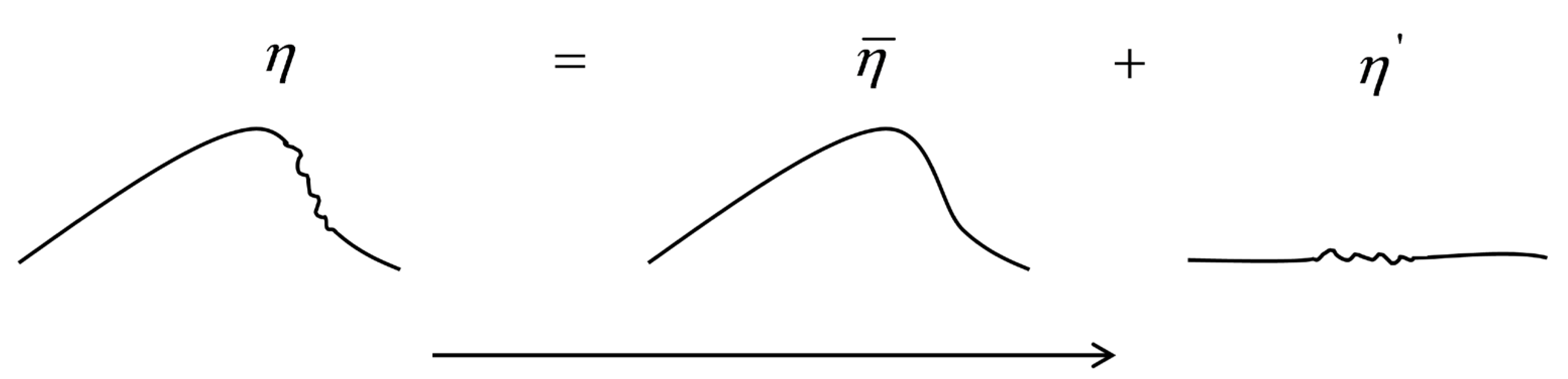
As mentioned in the introduction, the LWS method is based on the decomposition of flow variable scales to large and small ones, by the application of a volume filter to the velocity components and pressure, as in LES, and an exclusive surface filtering operation to the free-surface elevation. Specifically, each flow variable, f, is decomposed into resolved (large), $\overline{f}$, and subgrid (small), f′, scales, in a manner illustrated in Figure 1 for the decomposition of the free-surface elevation, η.

The implementation of the filtering operation in Equations (10) and (11) results, respectively, in the following governing equations for the resolved scales of the flow:

$${\displaystyle \frac{\partial {\overline{u}}_k}{\partial s_k}}+{\displaystyle \frac{2}{d+\overline{\eta }}}\left({\displaystyle \frac{\partial {\overline{u}}_3}{\partial s_3}}-{\overline{r}}_k{\displaystyle \frac{\partial {\overline{u}}_k}{\partial s_3}}\right)=0$$

(15)

$${\displaystyle \frac{\partial {\overline{u}}_i}{\partial t}}-{\displaystyle \frac{1+s_3}{d+\overline{\eta }}}{\displaystyle \frac{\partial \overline{\eta }}{\partial t}}{\displaystyle \frac{\partial {\overline{u}}_i}{\partial s_3}}+{\overline{u}}_k{\displaystyle \frac{\partial {\overline{u}}_i}{\partial s_k}}+{\displaystyle \frac{2}{d+\overline{\eta }}}\left({\overline{u}}_3-{\overline{r}}_k{\overline{u}}_k\right){\displaystyle \frac{\partial {\overline{u}}_i}{\partial s_3}}={\overline{P}}_i+{\displaystyle \frac{1}{{\mathrm{Re}}_d}}\left[{\displaystyle \frac{{\partial }^2{\overline{u}}_i}{\partial s_k\partial s_k}}+{\displaystyle \frac{4}{{\left(d+\overline{\eta }\right)}^2}}\left({\overline{r}}_k{\overline{r}}_k+1\right){\displaystyle \frac{{\partial }^2{\overline{u}}_i}{\partial s_3^2}}+{\overline{V}}_i\right]+{\overline{T}}_i$$

(16)

where the term

$${\overline{T}}_i=-{\displaystyle \frac{\partial {\tau }_{ik}}{\partial s_k}}-{\displaystyle \frac{2}{d+\overline{\eta }}}{\displaystyle \frac{\partial {\tau }_{i3}}{\partial s_3}}+{\displaystyle \frac{1+s_3}{d+\overline{\eta }}}{\displaystyle \frac{\partial {\tau }_{i3}^{\eta }}{\partial s_3}}-{\displaystyle \frac{1-s_3}{d+\overline{\eta }}}{\displaystyle \frac{\partial {\tau }_{ik}}{\partial s_3}}{\displaystyle \frac{\partial d}{\partial s_k}}$$

(17)

includes the subgrid scale (SGS) terms, i.e., the eddy SGS stresses and the wave SGS stresses, which, respectively, are as follows:

$${\tau }_{ij}=\overline{u_i{u}_j}-{\overline{u}}_i{\overline{u}}_j$$

(18)

$${\tau }_{i3}^{\eta }=\overline{u_i{u}_k{\displaystyle \frac{\partial \eta }{\partial s_k}}}-{\overline{u}}_i{\overline{u}}_k{\displaystyle \frac{\partial \overline{\eta }}{\partial s_k}}+\overline{u_i{\displaystyle \frac{\partial \eta }{\partial t}}}-{\overline{u}}_i{\displaystyle \frac{\partial \overline{\eta }}{\partial t}}+\overline{p{\displaystyle \frac{\partial \eta }{\partial s_i}}}-\overline{p}{\displaystyle \frac{\partial \overline{\eta }}{\partial s_i}}$$

(19)

Note that the eddy SGS stresses appear both in the LES and the LWS method, while the wave SGS stresses appear exclusively in the LWS method. It is noted that the filtering process takes into account some simplifying assumptions, which are presented in detail in Dimakopoulos and Dimas [39]. In addition, here it is considered $\overline{s_3^{2}f}=s_3^2\overline{f}$ due to the cut-off Chebyshev filter, which is used in the vertical direction (see Section 3), while the SGS terms, which result from the filtering of the viscous terms of Equation (11), are considered to be negligible compared to the ones of the convective terms.

The transformation of the coordinates, given by Equation (9), and the filtering procedure are also applied successively to the boundary conditions (3)–(8) at the free surface (s₃ = 1):

$${\overline{u}}_3={\displaystyle \frac{\partial \overline{\eta }}{\partial t}}+{\overline{u}}_k{\displaystyle \frac{\partial \overline{\eta }}{\partial s_k}}$$

(20)

$$p={\displaystyle \frac{\overline{\eta }}{{\mathrm{Fr}}^2}}+{\displaystyle \frac{1}{{\mathrm{Re}}_d}}\left[{\displaystyle \frac{2}{d+\overline{\eta }}}\left(2+{\displaystyle \frac{\partial \overline{\eta }}{\partial s_k}}{\displaystyle \frac{\partial \overline{\eta }}{\partial s_k}}\right){\displaystyle \frac{\partial {\overline{u}}_3}{\partial s_3}}-{\displaystyle \frac{\partial \overline{\eta }}{\partial s_k}}\left({\displaystyle \frac{2}{d+\overline{\eta }}}{\displaystyle \frac{\partial {\overline{u}}_k}{\partial s_3}}+{\displaystyle \frac{\partial {\overline{u}}_3}{\partial s_k}}\right)\right]$$

(21)

$$-2{\displaystyle \frac{\partial \overline{\eta }}{\partial s_1}}{\displaystyle \frac{\partial {\overline{u}}_1}{\partial s_1}}-{\displaystyle \frac{\partial \overline{\eta }}{\partial s_2}}\left({\displaystyle \frac{\partial {\overline{u}}_1}{\partial s_2}}+{\displaystyle \frac{\partial {\overline{u}}_2}{\partial s_1}}\right)+{\displaystyle \frac{2}{d+\overline{\eta }}}\left({\displaystyle \frac{\partial {\overline{u}}_1}{\partial s_3}}+{\displaystyle \frac{\partial \overline{\eta }}{\partial s_1}}{\displaystyle \frac{\partial {\overline{u}}_3}{\partial s_3}}\right)\left(1+{\displaystyle \frac{\partial \overline{\eta }}{\partial s_k}}{\displaystyle \frac{\partial \overline{\eta }}{\partial s_k}}\right)+\left[1-{\left({\displaystyle \frac{\partial \overline{\eta }}{\partial s_1}}\right)}^2\right]{\displaystyle \frac{\partial {\overline{u}}_3}{\partial s_1}}+{\displaystyle \frac{\partial \overline{\eta }}{\partial s_1}}{\displaystyle \frac{\partial \overline{\eta }}{\partial s_2}}{\displaystyle \frac{\partial {\overline{u}}_3}{\partial s_2}}=0$$

(22)

$$-2{\displaystyle \frac{\partial \overline{\eta }}{\partial s_2}}{\displaystyle \frac{\partial {\overline{u}}_2}{\partial s_2}}-{\displaystyle \frac{\partial \overline{\eta }}{\partial s_1}}\left({\displaystyle \frac{\partial {\overline{u}}_1}{\partial s_2}}+{\displaystyle \frac{\partial {\overline{u}}_2}{\partial s_1}}\right)+{\displaystyle \frac{2}{d+\overline{\eta }}}\left({\displaystyle \frac{\partial {\overline{u}}_2}{\partial s_3}}+{\displaystyle \frac{\partial \overline{\eta }}{\partial s_2}}{\displaystyle \frac{\partial {\overline{u}}_3}{\partial s_3}}\right)\left(1+{\displaystyle \frac{\partial \overline{\eta }}{\partial s_k}}{\displaystyle \frac{\partial \overline{\eta }}{\partial s_k}}\right)+\left[1-{\left({\displaystyle \frac{\partial \overline{\eta }}{\partial s_2}}\right)}^2\right]{\displaystyle \frac{\partial {\overline{u}}_3}{\partial s_2}}+{\displaystyle \frac{\partial \overline{\eta }}{\partial s_1}}{\displaystyle \frac{\partial \overline{\eta }}{\partial s_2}}{\displaystyle \frac{\partial {\overline{u}}_3}{\partial s_1}}=0$$

(23)

and the bed (s₃ = −1):

$${\overline{u}}_1-{\overline{u}}_3{\displaystyle \frac{\partial d}{\partial s_1}}=0, {\overline{u}}_2-{\overline{u}}_3{\displaystyle \frac{\partial d}{\partial s_2}}=0$$

(24)

$${\overline{u}}_3+{\overline{u}}_k{\displaystyle \frac{\partial d}{\partial s_k}}=0$$

(25)

Note that in Equations (20)–(25), the effect of the subgrid scales, resulting from the filtering procedure, is considered to be negligible.

In the present study, the eddy and wave SGS stresses, appearing in Equation (17), are computed by use of Smagorinsky eddy-viscosity models [40]. Specifically, the model for the eddy SGS stresses is as follows:

$${\tau }_{ij}=-2{\nu }_{\tau }{\overline{S}}_{ij}=-2C_s^2{\Delta }^2\left|\overline{S}\right|{\overline{S}}_{ij}$$

(26)

where C_s = 0.1 is the model parameter (its value is set according to the usual practice in LES), Δ = (Δs₁Δs₂Δs₃)^1/3 is the smallest resolved scale based on the grid size, ${\overline{S}}_{ij}$ is the strain-rate tensor of resolved scales

$${\overline{S}}_{ij}={\displaystyle \frac{1}{2}}\left({\displaystyle \frac{\partial {\overline{u}}_i}{\partial s_j}}+{\displaystyle \frac{\partial {\overline{u}}_j}{\partial s_i}}\right)$$

(27)

and $\left|\overline{S}\right|={\left(2{\overline{S}}_{ij}{\overline{S}}_{ij}\right)}^{1/2}$. The model for the wave SGS stresses, based on the one presented in Dimas and Fialkowski [39], is as follows:

$${\tau }_{ij}^{\eta }=-2{\nu }_{\tau }^{\eta }{\overline{S}}_{ij}^{\eta }=-2C_{\eta }^2{\Delta }^2\left|{\overline{S}}^{\eta }\right|{\overline{S}}_{ij}^{\eta }$$

(28)

where C_η is the model parameter and ${\overline{S}}_{ij}^{\eta }$ is a modified strain-rate tensor involving free-surface resolved scales:

$${\overline{S}}_{ij}^{\eta }={\delta }_{3j}{\overline{S}}_{ik}\left|{\displaystyle \frac{\partial \overline{\eta }}{\partial s_k}}\right|$$

(29)

where δ_ij is the Kronecker delta, and $\left|{\overline{S}}^{\eta }\right|={\left(2{\overline{S}}_{ij}^{\eta }{\overline{S}}_{ij}^{\eta }\right)}^{1/2}$.

An issue that arises when eddy-viscosity models are applied for the SGS stresses computation is the behavior of the eddy viscosities, ν_τ and ν_τ^η, close to the bed, which often is the source of instabilities during the numerical solution of flow equations. For this reason, an exponentially decaying function is used to multiply the eddy viscosities, based on the one proposed in Piomelli and Balaras [41], whose value tends to 1 far from solid boundaries and becomes exactly equal to zero at solid boundaries.

The calibration and sensitivity analysis of the wave SGS parameter, C_η, was performed by Dimakopoulos and Dimas [39], who utilized the LWS method, coupled with the Euler equations (inviscid flow) for the simulation of spilling breakers. After comparison of their numerical results to corresponding experimental measurements [26,42], it was concluded that the best balanced behavior was achieved for C_η = 0.4; a value that is also adopted in the present work.

3. Numerical Setup

The flow simulations are based on the numerical solution of the transformed Navier–Stokes equations using a fractional time-step scheme for the temporal discretization, and a hybrid scheme for the spatial discretization. The hybrid scheme comprises central finite differences, on a uniform grid with size Δs₁, for the discretization along the cross-shore direction s₁, a pseudo-spectral approximation method with Fourier modes along the longshore direction s₂, and a pseudo-spectral approximation method with Chebyshev polynomials along the vertical direction s₃.

Then, an extra transformation of the velocity components, i.e., ${\overline{v}}_i={\overline{u}}_i-{\delta }_{3i}{\overline{r}}_k{\overline{u}}_k$, is performed in order to obtain a compact form of the flow equations and facilitate their efficient numerical solution by a time-splitting scheme for their temporal discretization. After implementing this transformation, the continuity (15) and the Navier–Stokes Equation (16), respectively, take the following form:

$${\partial }_j^T{\overline{v}}_j+{\displaystyle \frac{2}{d+\overline{\eta }}}{\overline{v}}_k{\displaystyle \frac{\partial {\overline{r}}_k}{\partial s_3}}=0$$

(30)

$${\displaystyle \frac{\partial {\overline{v}}_i}{\partial t}}={\epsilon }_{ijm}{\overline{v}}_j{\overline{\zeta }}_m+{\overline{A}}_i-{\partial }_i^T\overline{\mathsf{\Pi }}+{\displaystyle \frac{1}{{\mathrm{Re}}_d}}\left({\partial }_j^{2,T}{\overline{v}}_i+{\overline{V}}_i\right)+{\overline{T}}_i$$

(31)

where m = 1, 2, 3 and ε_ijm = (i − j)(j − m)(m − i)/2 is the Levi-Civita tensor, which is equal to either +1, or −1, depending on the position of the indices (i, j, q), and equal to zero whenever one of the indices is repeated. Also, ${\overline{\zeta }}_m={\epsilon }_{ijm}{\partial }_j^T{\overline{v}}_m$ is the transformed vorticity, $\overline{\mathsf{\Pi }}=\overline{p}+0.5{\overline{v}}_j{\overline{v}}_j$ is the transformed pressure head,

$$\begin{array}{c}{\partial }_j^T=\left[{\displaystyle \frac{\partial }{\partial s_1}}, {\displaystyle \frac{\partial }{\partial s_2}}, {\displaystyle \frac{2}{d+\overline{\eta }}}{\displaystyle \frac{\partial }{\partial s_3}}\right]\\ {\partial }_j^{2,T}=\left[{\displaystyle \frac{{\partial }^2}{\partial s_1^2}}, {\displaystyle \frac{{\partial }^2}{\partial s_2^2}}, {\left({\displaystyle \frac{2}{d+\overline{\eta }}}\right)}^2{\displaystyle \frac{{\partial }^2}{\partial s_3^2}}\right]\end{array}$$

(32)

are the transformed first and second derivative operators, respectively,

$$\begin{array}{c}{\overline{A}}_k=0.5\left(1+s_3\right)\left(\partial \overline{\eta }/\partial t\right){\partial }_3^T{\overline{v}}_k+{\overline{r}}_k{\partial }_3^T\overline{p}\\ {\overline{A}}_3=0.5\left(1+s_3\right)\left(\partial \overline{\eta }/\partial t\right){\partial }_3^T\left({\overline{v}}_3+{\overline{r}}_k{\overline{v}}_k\right)-\partial \left({\overline{r}}_k{\overline{v}}_k\right)/\partial t-{\overline{v}}_j{\partial }_j^T\left({\overline{r}}_k{\overline{v}}_k\right)\end{array}$$

(33)

are the nonlinear terms, while the part of the viscous terms resulting from the flow equations transformation is expressed as follows:

$$\begin{array}{c}{\overline{V}}_l={\overline{r}}_k{\overline{r}}_k{\partial }_{3,2}^T{\overline{v}}_l-2{\overline{r}}_k{\partial }_3^T\left({\partial }_k^T{\overline{v}}_l\right)-\left({\partial }_k^T{\overline{r}}_k-2{\overline{r}}_k{\partial }_3^T{\overline{r}}_k\right){\partial }_3^T{\overline{v}}_l , l=1,2\\ {\overline{V}}_3={\overline{r}}_k{\overline{r}}_k{\partial }_{3,2}^T{\overline{v}}_3+\left(1+{\overline{r}}_k{\overline{r}}_k\right){\partial }_{3,2}^T\left({\overline{r}}_l{\overline{v}}_l\right)-2{\overline{r}}_k{\partial }_k^T\left[{\partial }_3^T\left({\overline{v}}_3+{\overline{r}}_l{\overline{v}}_l\right)\right]-\left({\partial }_k^T{\overline{r}}_k-2{\overline{r}}_k{\partial }_3^T{\overline{r}}_k\right){\partial }_3^T\left({\overline{v}}_3+{\overline{r}}_l{\overline{v}}_l\right)\end{array}$$

(34)

Similar expressions are derived for the transformed boundary conditions, Equations (20)–(25).

The time-splitting scheme for the temporal discretization comprises three stages per time step, where the computation of the velocity field is achieved by adding the corresponding corrections at each of the three stages to the field of the previous time step. Moreover, the dynamic pressure field is obtained in the second stage of each time step, while the free-surface elevation is computed at the end of each time step using the kinematic, free-surface boundary condition.

At the first stage of each time step, the nonlinear term, $\overline{A}$, the SGS term, $\overline{T}$, and the viscous term, $\overline{V}$, of the transformed equations of motion (30) are treated explicitly. At the second stage, an implicit Euler scheme is used for the treatment of the pressure head term, ${\partial }_i^T\overline{\mathsf{\Pi }}$, of Equation (30), which results in a generalized Poisson’s equation for Π by satisfying the transformed continuity equation as well. The transformed dynamic (normal stress) free-surface condition and non-penetration bottom condition are imposed at this stage. At the third stage, the remaining viscous terms, ${\partial }_j^{2,T}{\overline{v}}_i$, are treated by an Euler implicit scheme satisfying the transformed dynamic (tangential stress) free-surface and bottom conditions.

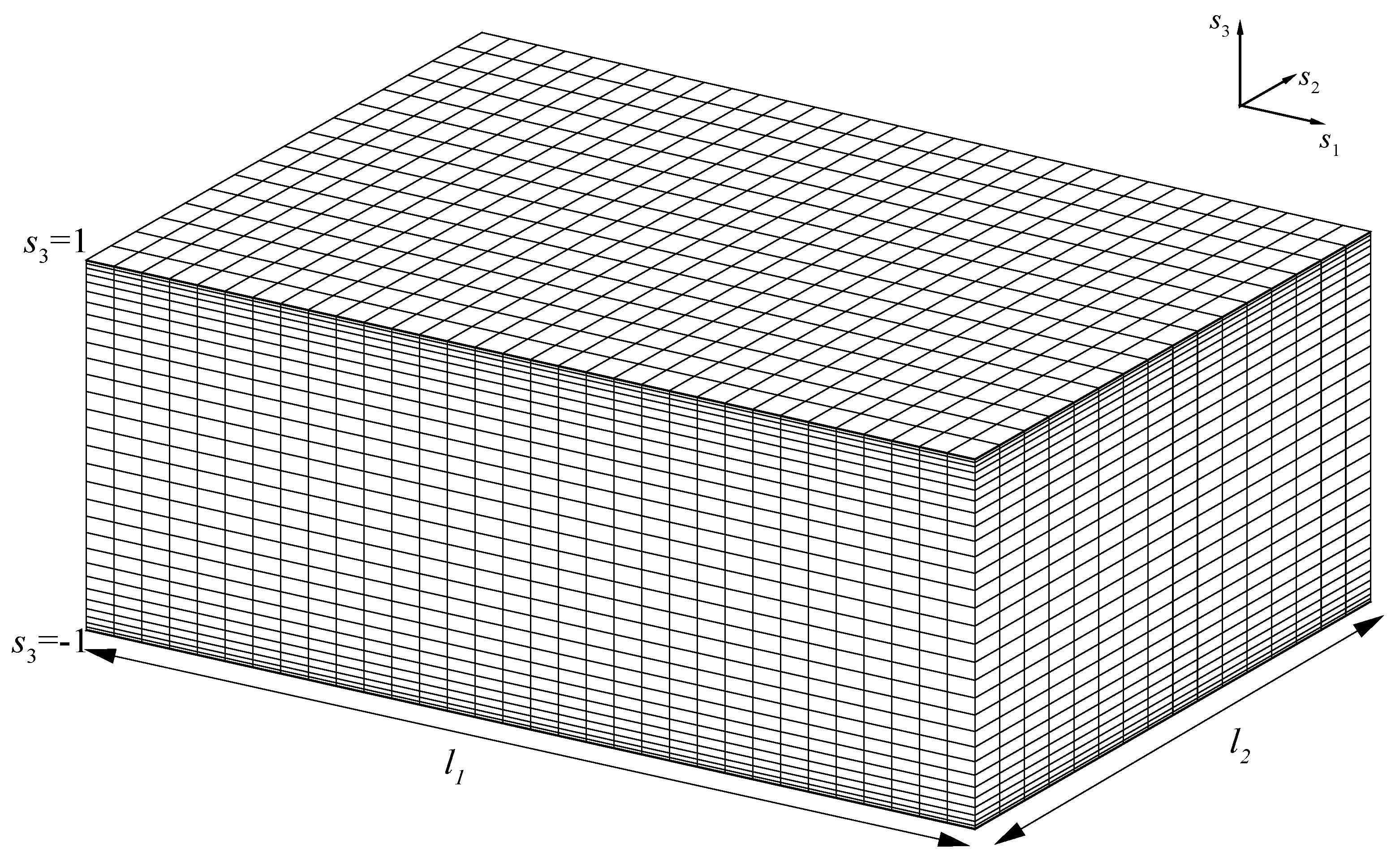
According to the utilized hybrid scheme, the spatial discretization is applied on a grid (Figure 2) of L finite-difference cells, M Fourier modes, and N + 1 Chebyshev nodes, where each flow variable $\overline{f}$ (velocity components and pressure) is approximated by the expression:

$$\overline{f}\left(s_1,s_2,s_3,t\right)={\displaystyle \sum _{m=-M/2}^{M/2-1}{\displaystyle \sum _{n=0}^N{\tilde{f}}_{lmn}\left(t\right)}}\exp \left(-2\pi i{\displaystyle \frac{m{s}_2}{l_2}}\right)T_n\left(s_3\right)$$

(35)

where ${\tilde{f}}_{lmn}$ is the Chebyshev-Fourier transformation of $\overline{f}$, l is the node index in s₁, i is the imaginary unit, l₂ = M∙Δs₂, is the length of the computational domain in s₂, Δs₂ is the grid size in s₂, T_n is the Chebyshev polynomial of order n, and N is the highest order of the Chebyshev polynomials. In the s₃ direction, the solution is obtained on the Chebyshev-Gauss-Lobatto collocation points [43], the intrinsic property of which is the refinement of the grid in the vicinity of boundaries [44]. The transformations between physical and spectral space are performed by a Fast Fourier Transform algorithm [45]. Given the spectral character of the discretization method, the filtering operation to obtain the flow Equations (15) and (16) for the resolved scales is implemented by using a sharp spectral filter [46].

The implementation of Equation (35) for the discretization of Equation (31) leads to the formation of a system of (L + 1)(Ν + 1)M algebraic equations, with the general form $\left[B\right]\times \left[\tilde{f}\right]=\left[\tilde{b}\right]$, for each of the transformed flow variables (pressure and velocities). Each of these systems may be divided into M independent subsystems ($\left[B_m\right]\times \left[{\tilde{f}}_m\right]=\left[{\tilde{b}}_m\right]$, one for each Fourier mode), which can be solved in parallel due to the decoupling of the Fourier modes. In the present study, parallelization is performed by means of OpenMP directives [47], while each subsystem is solved at every time step using an iterative generalized Gauss-Seidel method. The matrix of coefficients $\left[B_m\right]$ is a band diagonal and is decomposed once at the beginning of the computation by using the LU-decomposition method. The three-dimensional simulations presented in this study were performed exclusively in parallel on 64 CPU AMD Opteron^(TM) rack servers, and a typical run required approximately 10⁻⁶ s per grid node and time step. Note also that the total simulation period of a typical run was equal to about 40 wave periods; the first 20 periods to reach a fully developed state in terms of the wave propagation, and the latter 20 periods in order to obtain period-averaged results.

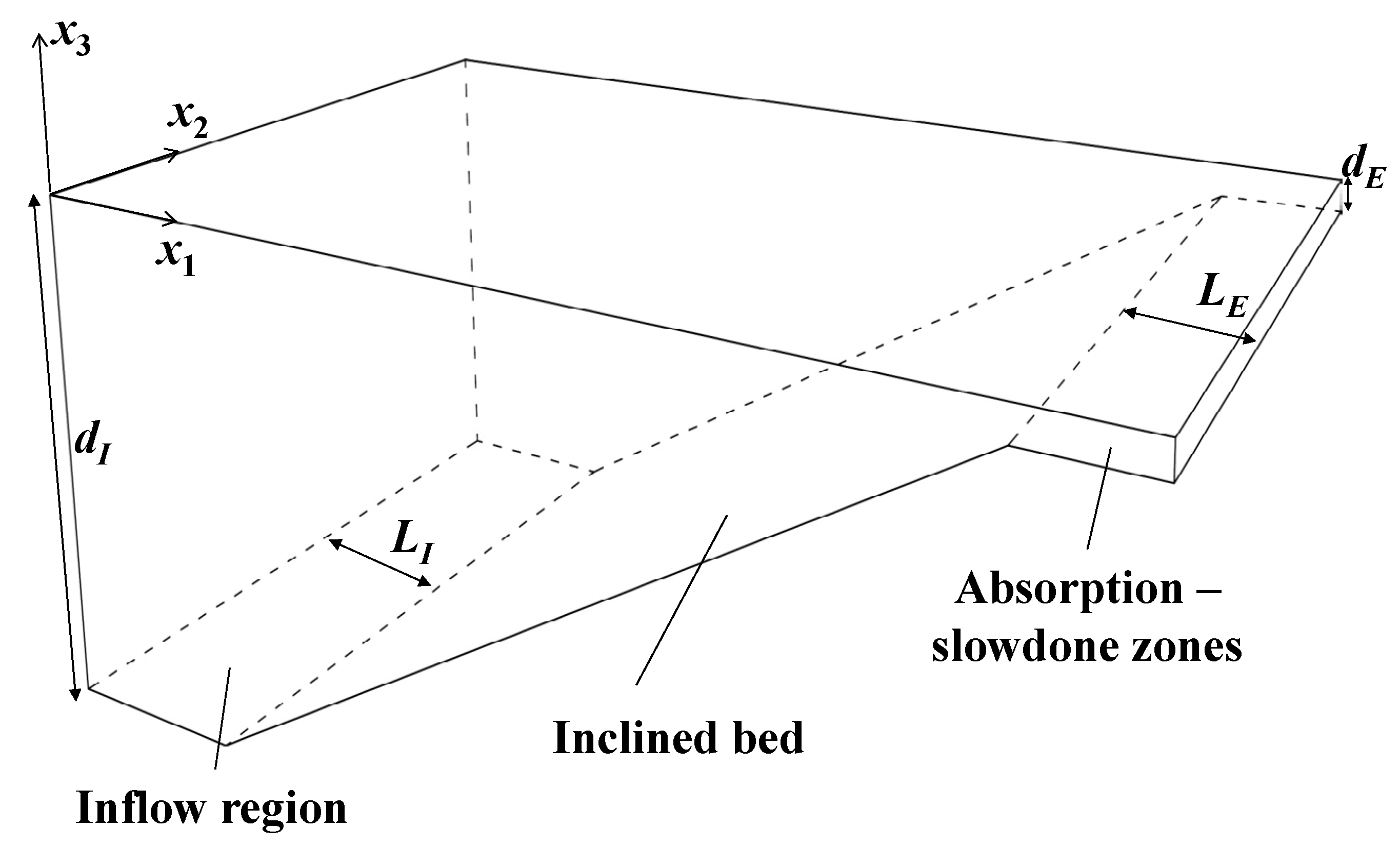
In the present work, the propagation, transformation, and spilling breaking of incoming second-order Stokes waves over a constant slope bed are simulated. As shown in the sketch of the computational domain (Figure 3), a flat-bed region of length L_I and constant depth d_I, which ensures the development of the incoming waves, is followed by the inclined region of the bed. Then, a flat wave outflow region of length L_E and constant depth d_E << d_I (the formulation allows the outflow depth d_E to be very small but nonzero) is considered in order to model the effect of the swash zone of a coastal area, where the waves are gradually completely dissipated. For this reason, two overlapping actions are considered in the wave outflow region: a wave absorption model, which ensures that waves are not reflected by the outflow boundary [48], and a velocity attenuation (slowdown) model, which is activated by increasing the kinematic viscosity, i.e., reducing the value of the Re_d, in the numerical solution of Equation (31). In addition, periodic boundary conditions are imposed in the s₂ direction, an intrinsic property of the Fourier approximation.

4. Results

4.1. Validation of the Numerical Model

The accuracy of the model, including an inviscid version of the solver for the Euler equations, and also the efficiency of the wave absorption at the outflow region, was verified in Dimas and Dimakopoulos [39], who simulated cases of non-breaking waves propagating normally and obliquely to the shore. In the same paper, the LWS method implemented in an inviscid flow solver was calibrated and verified by simulating a spilling wave breaker case (cross-shore incidence) and comparing the numerical results to corresponding experimental data [26,42].

In the present study, a three-dimensional numerical simulation of the normal to the shoreline propagation and spilling breaking of incident second-order Stokes waves over a bed of constant slope tan β = 1/35 was performed in order to examine the accuracy and efficiency of the viscous version of the LWS method, i.e., implemented with the Navier–Stokes equations. The numerical results are longshore-averaged and then compared to the corresponding experimental results in Ting and Kirby [26].

The laboratory measurements in Ting and Kirby [26], which were conducted in a wave tank of length, width, and depth equal to 40 m, 0.6 m, and 1 m, respectively, involved cases of spilling and plunging breakers. The experimental flow parameters for the case of spilling breaking, which is considered here, are summarized as: wave inflow depth, d_I = 0.4 m, and wave height and period, H_I = 0.125 m and Τ = 2 s, respectively, which correspond to wave height and wavelength, H_ο = 0.127 m and λ_ο = 6.245 m, respectively, at deep water. In the present model, the wave parameters at deep water are identical to those in Ting and Kirby [26], but a larger inflow depth d_I = 0.7 m is considered (since the Stokes wave theory is utilized for the incident waves), where the wave height is H_I = 0.118 m based on shoaling. The parameters of the incoming waves are rendered dimensionless by d_I, g, and the resulting values are H_I = 0.168, Τ = 7.487, and λ_I = 6.605. The Irribaren number is ξ_ο = tanβ(λ_ο/H_ο)^1/2 = 0.2, which corresponds to a spilling breaker of medium strength, while a value of Re_d = 250,000 is considered. The total length of the computational domain is L_T = 60, the flat inflow region has length L_I = 15, while the wave outflow region is of length L_E = 11.05 and depth d_E = 0.03. The lengths of the wave absorption and the velocity attenuation regions are L_A = 11 and L_D = 2, respectively. The numerical parameters are: Δs₁ = 0.04, N = 64, M = 128, Δs₂ = 0.103, and Δt = 5∙10⁻⁴.

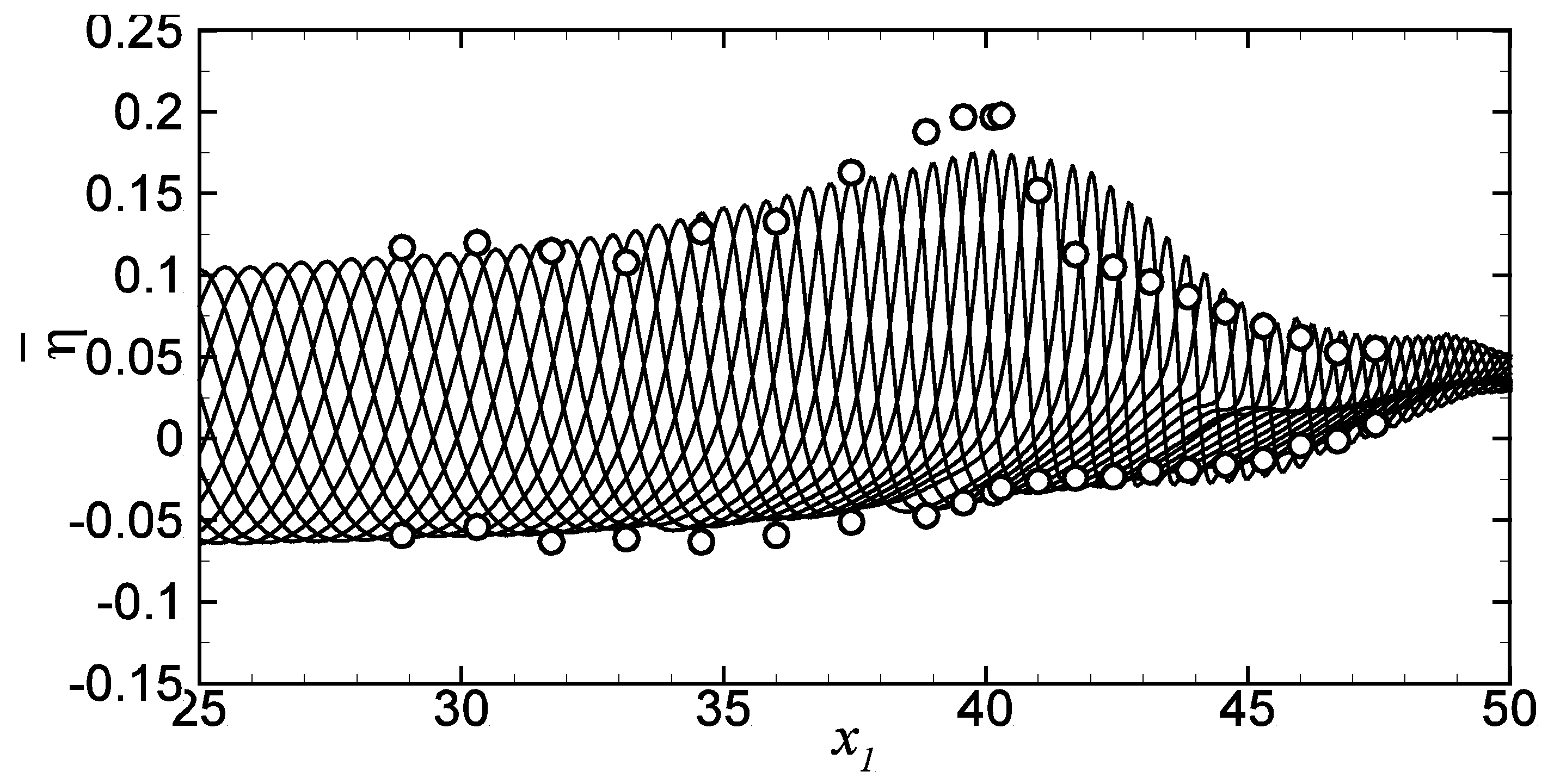
In Figure 4, snapshots of the resolved free-surface elevation, $\overline{\eta }$, at several time instants after about 30 wave periods, are presented and compared to the experimental measurements of maximum (wave crest) and minimum (wave trough) values of the free surface elevation [26]. The numerical model predicts accurately the breaking depth, d_b = 0.28, which corresponds to the position x₁ = 40.2, but underestimates the breaking height, as indicated by the deviation of the breaking free-surface elevation, ${\overline{\eta }}_b=0.176$, calculated by the LWS model, in comparison to the experimental one, ${\overline{\eta }}_b=0.196$, by about 9%. This prediction is still better than the ones in Lin and Liu [49], Bradford [25], and Christensen [1]. At the outer surf zone (40 < x₁ < 44), the numerical model underestimates the wave height dissipation, as opposed to the inner surf zone (x₁ > 44), where the prediction of the model for the height dissipation is very good. Also, the numerical results for the wave trough elevation are in very good agreement with the experimental data. Finally, in the surf zone, the numerical results fit the measured wave setup very well.

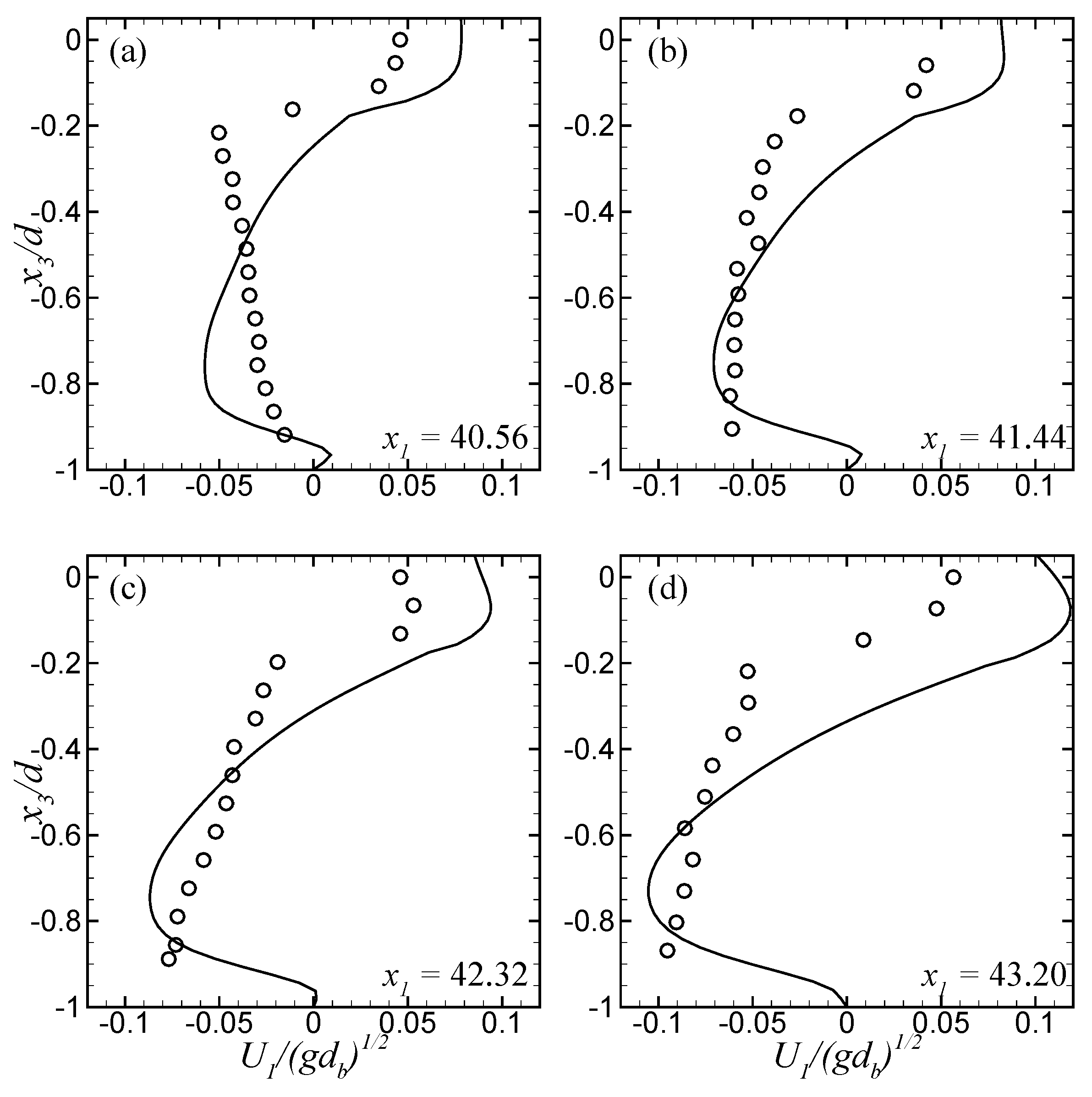
The resulting period-averaged velocity field (Figure 5) indicates that the numerical model is able to capture the undertow in the surf zone, the development of which is guided by the fact that the net cross-shore water flux in the surf zone is zero. In Figure 5, the mean velocity field in the surf zone indicates the presence of an onshore-directed current, which is due to the Eulerian drift and the presence of the surface roller in the upper layer of the water depth, and the offshore-directed undertow in the lower layer of the water depth, which balances the onshore flux. Very close to the bed, a steady current of weak strength, the so-called wave boundary layer streaming, exists offshore to the breaking region and part of the outer surf zone and is directed towards the shoreline. For the quantitative verification of the undertow, LWS-predicted vertical profiles at four locations in the surf zone (Figure 6) are compared to the corresponding experimental data presented in Figure 5 in Ting and Kirby [26] for the case of a spilling breaker. The period-averaged, horizontal velocity, U₁, is normalized with respect to g and the breaking depth, d_b. Overall, the LWS prediction is deemed adequate, since the order of magnitude as well as the gradient of the numerical profiles agree well with the experimental ones. A significant deviation is observed between numerical and measured profiles with respect to the depth where the velocity acquires its most negative value, as it is indicated in Figure 6c,d; this is attributed to the fact that the present Re_d value is about 7 times smaller than the one in the experiments.

4.2. Oblique Wave Breaking

Next, the three-dimensional, turbulent, free-surface flow, induced by wave propagation and breaking oblique to the shoreline and over a constant slope bed (tan β = 1/35), was numerically simulated, mainly in order to analyze the interaction between the longshore current and the undertow in the surf zone. Two cases are considered with wave incidence angles equal to φ_Ι = 20° and 30° at water depth d_I, which correspond to φ_o = 27.5° and 42.5°, respectively, at deep water. All other inflow wave parameters, the model parameters (C = 0.1 and C_η = 0.4), and the form of the computational domain (Figure 3), remain the same as in the validation case where φ_Ι = 0°. The numerical parameters are also identical to the ones of the cross-shore incidence case, i.e., Δs₁ = 0.04, N = 64, M = 128 (corresponding to Δs₂ = 0.151 and 0.103 for φ_Ι = 20° and 30°, respectively), and Δt = 5∙10⁻⁴. The width of the computational domain, L_F, is set equal to one longshore wavelength, λ₂ = λ_Ι/sinφ_Ι, in order to be compatible with the periodic boundary conditions in s₂, imposed by the approximation with Fourier modes, so L_F = 19.31 and 13.21 for φ_Ι = 20° and 30°, respectively.

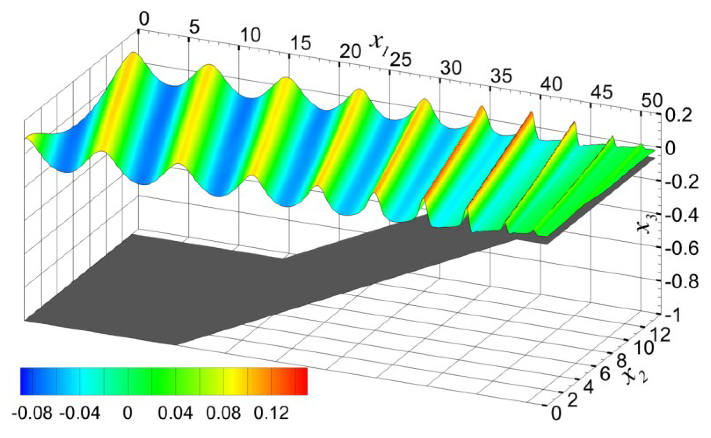
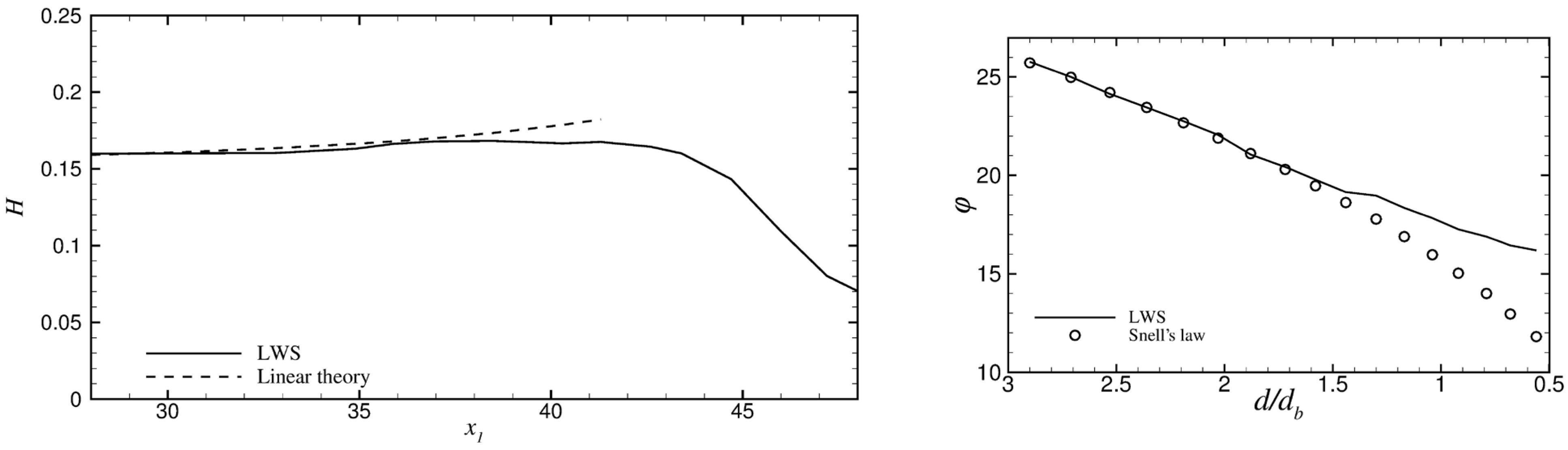
A typical snapshot of the free-surface elevation for the case of φ_Ι = 30°, is presented in Figure 7, where the bed of the computational domain is also shown. As clearly indicated, the combined action of nonlinear refraction and shoaling of waves is the mechanism that results in the wave transformation in the outer coastal zone. Next, gradual wave breaking in the longshore direction, due to the oblique incidence, takes place, which is followed by wave energy dissipation in the surf zone. It is found that, for both wave incidence angles, breaking initiates at d_b ≈ 0.25 (x₁ ≈ 41). The corresponding cross-shore distribution of the wave height, in comparison to linear wave shoaling and wave refraction based on Snell’s law, and the wave direction angle, in comparison to Snell’s law, is shown in Figure 8.

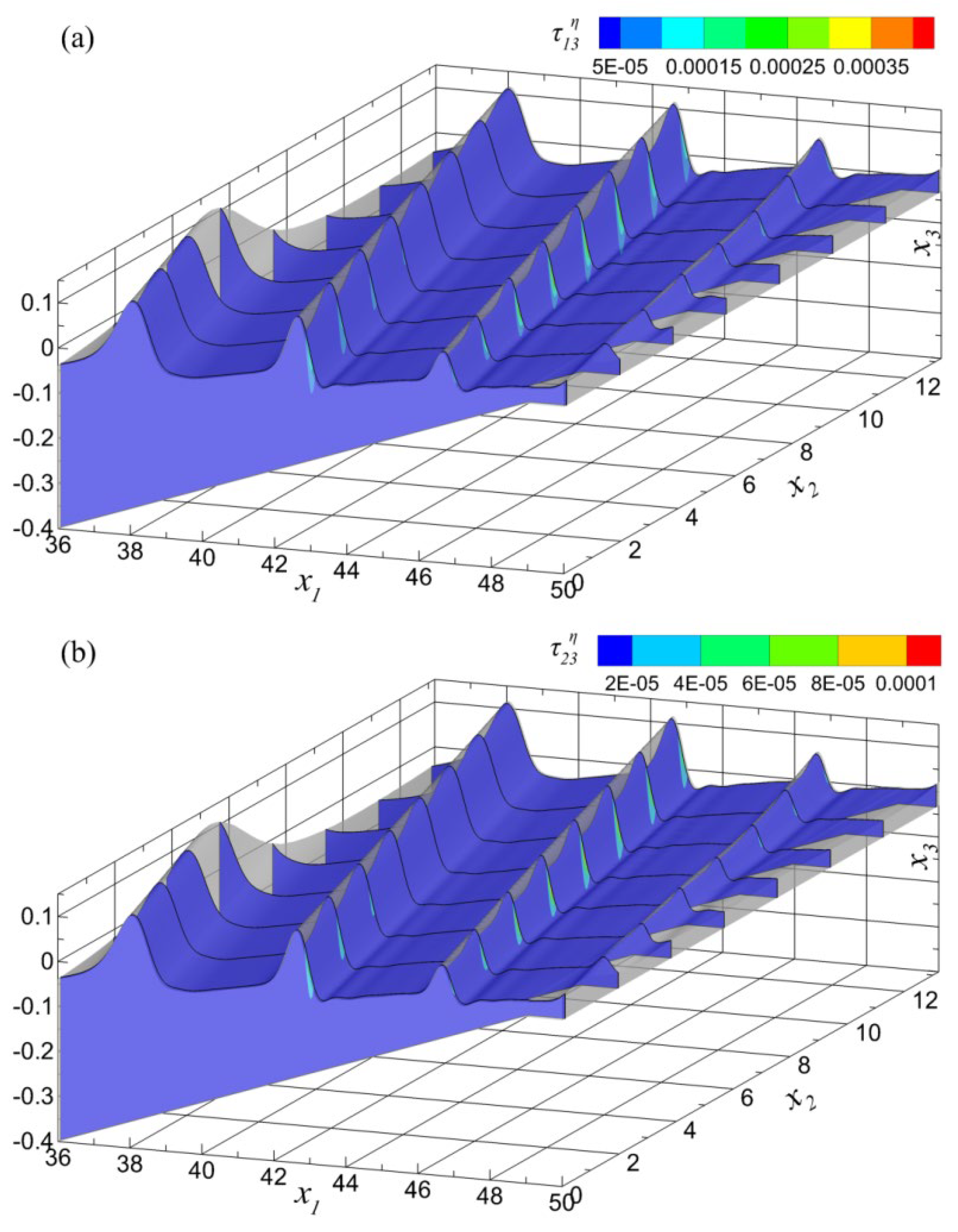
According to the LWS method, wave breaking and dissipation in the surf zone are coupled to the generation and combined action of the eddy and wave SGS stresses. The distribution of the wave stresses, τ₁₃^η and τ₂₃^η, which are the most significant SGS stresses, in terms of their magnitude, at several cross-sections in the surf zone, is presented in Figure 9 for the case of φ_Ι = 30°. The wave SGS stresses appear at incipient breaking, i.e., at x₁ ≈ 41, and acquire their maximum strength at depth d/d_b ≈ 0.5 (x₁ ≈ 45.5). For shallower water depths, the strength of the SGS stresses attenuates before they vanish in the inner surf zone. The development of the surface roller, accompanied by vorticity production, is connected to the development of the wave SGS stresses mainly in the vicinity of the obliquely breaking wavefront. It is noted that the eddy and wave SGS stresses behave in a similar fashion for φ_Ι = 20° as well.

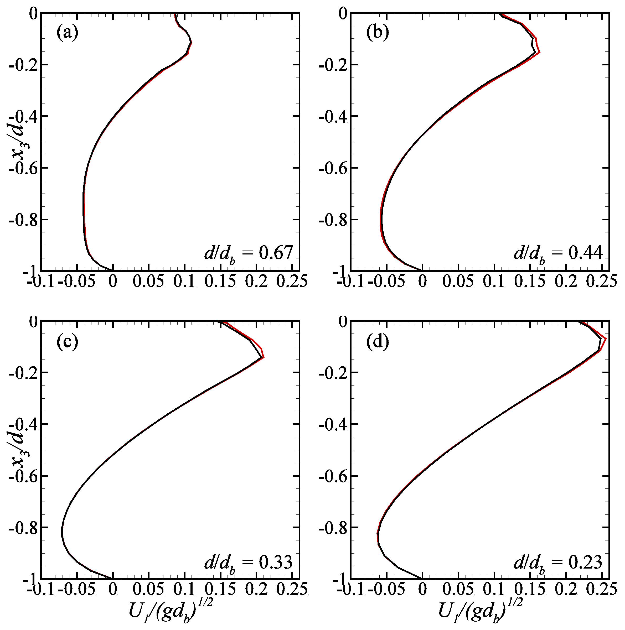
LWS-predicted vertical profiles of the longshore current and the undertow at four positions in the surf zone are presented, respectively, in Figure 10 and Figure 11, for both wave incidence angle, φ_Ι, cases. The period-averaged and longshore-averaged velocities, U₂ in the longshore direction and U₁ in the cross-shore direction, are normalized with respect to the breaking depth, d_b, as in the validation case.

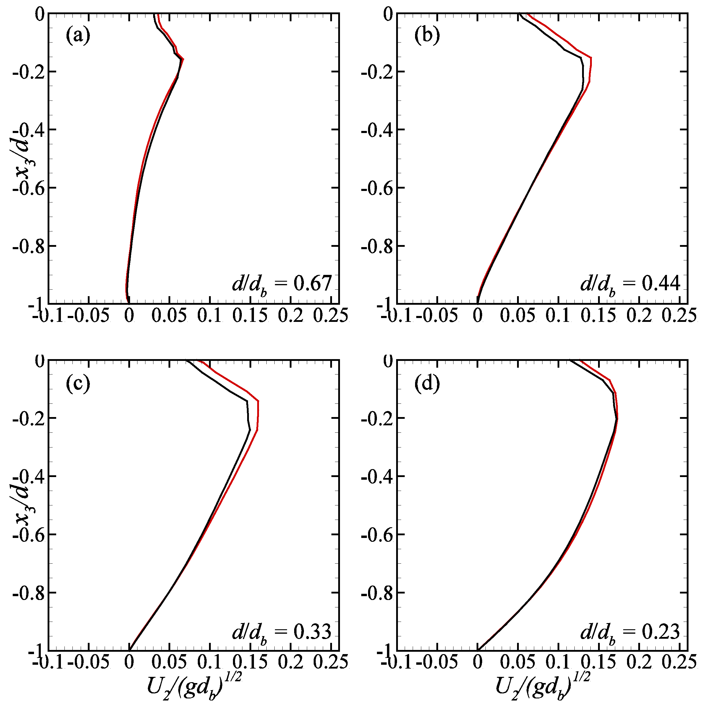
For the longshore current, it is shown (Figure 10) that it becomes stronger shorewards of the breaking depth. The longshore current vertical profiles have positive U₂ values over the whole depth, as expected, with local maxima close to the free surface. As shown in Figure 10a–c, the U₂ distribution over the depth seems to be linear between the bed bottom and the wave trough, while at shallower depths (Figure 10d), it tends to be logarithmic. Note that the longshore current vertical profiles for the case with φ_Ι = 20° present slightly smaller maxima compared to the corresponding ones for φ_Ι = 30°.

For the undertow, it is shown (Figure 11) that the vertical profiles, corresponding to the two different wave incidence angles φ_Ι = 20° and 30°, are almost identical, probably due to the relatively small difference between the considered φ_Ι values. In general, the corresponding undertow vertical profiles do not differ much from those of the cross-shore wave incidence case (Figure 6), presenting a strong onshore current near the bed and a magnitude of the same order. The major difference (see Figure 6 and Figure 11) is that in the case of oblique breaking, the magnitude of the undertow, at each location, has its maximum value closer to the bed compared to the cross-shore breaking, a result that is connected to the shoreward displacement of breaking in the oblique wave cases.

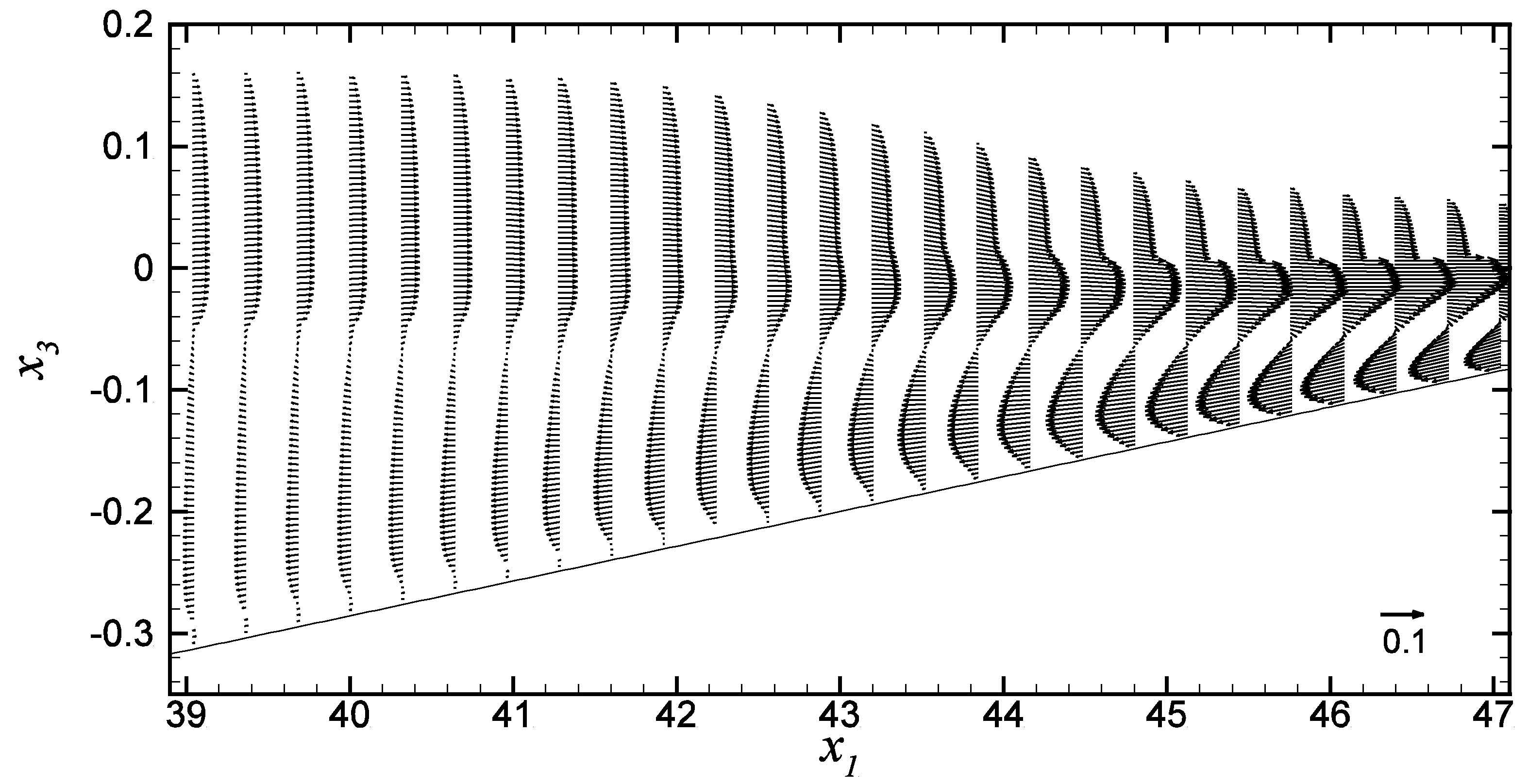
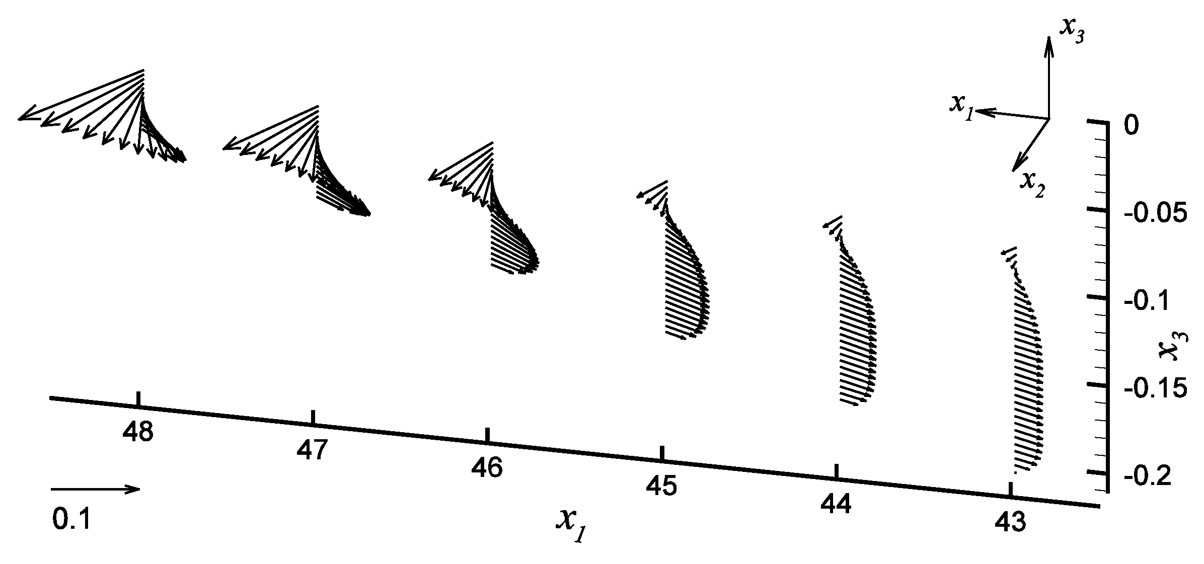
In Figure 12, the vertical distribution of the period and longshore-averaged velocity vectors, at six positions in the surf zone for the case of φ_Ι = 30°, is presented. The three deeper distributions (x₁ = 43–45) clearly indicate that the undertow dominates in the outer surf zone, since the offshore-directed velocity occupies the majority of the water column. On the contrary, at shallower water depths (x₁ = 46–48), the magnitude of the longshore current is enhanced, as indicated by the gradual increase and turning of the mean velocity vectors towards the parallel to the shoreline direction. Note that, as mentioned above (Figure 9), the wave SGS stresses acquire their maximum strength at x₁ ≈ 45.5.

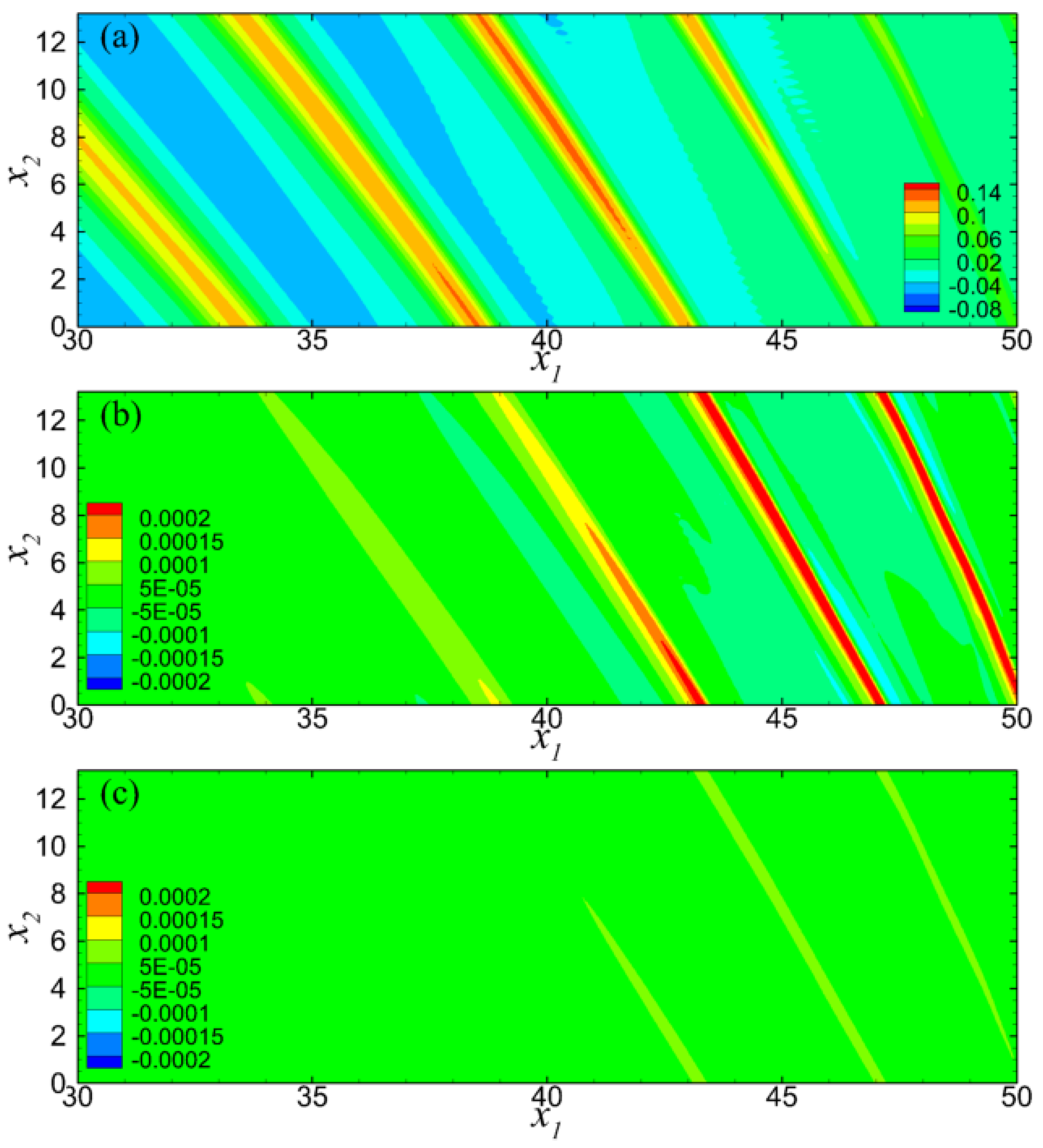
Finally, in Figure 13, a typical plan view of the resolved free-surface elevation contours and contours of the cross-shore and longshore bed shear stress components, τ_b1 and τ_b2, respectively, are presented (for φ_Ι = 30°). For both τ_b1 and τ_b2, the amplitude of their spatial variation is gradually increasing over the sloping bed, especially at breaking and in the surf zone (for x₁ > 41.5). Obviously, the cross-shore component of the bed shear stress reaches higher maximum and minimum values compared to the longshore one. The magnitude of both bed shear stresses decreases in the inner surf zone, following the wave height attenuation, while the decrease in the wavelength indicated by the decreasing distance between successive wave crestlines (Figure 13a) is “transmitted” to the spatial variation in τ_b1 and τ_b2, as shown in Figure 13b,c.

5. Conclusions

A numerical model for the simulation of wave propagation (normal and oblique to the shore) and spilling breaking over a constant slope bed is presented. The model is based on the implementation of the LWS method in a numerical solver of the three-dimensional Navier–Stokes equations. According to the LWS method, the wave and eddy SGS stresses are modeled by use of eddy-viscosity models and then introduced to the viscous flow solver in order to model the effect of subgrid flow and free-surface elevation scales on wave breaking and wave energy dissipation in the surf zone.

The combined effect of nonlinear refraction and shoaling of waves is captured by the model, for the case of oblique wave incidence, considering two cases with wave incidence angles equal to φ_Ι = 20° and 30°. The development of the surface roller in the breaking wavefront is connected to the increase in the strength of the SGS stresses in the outer surf zone and their successive decrease at shallower depths close to the shore.

For both of the investigated cases (φ_Ι = 20° and 30°), vertical profiles of the longshore current and the undertow at several locations in the surf zone are presented. As expected, the undertow profiles indicate the presence of a strong onshore current close to the bed, while the longshore current profiles show the generation of a current in the positive longshore direction, over the whole depth. The difference between the inflow wave angles does not seem to affect the undertow distribution in the surf zone, while the longshore current profiles for φ_Ι = 30° demonstrate slightly larger maxima than the corresponding ones for φ_Ι = 20°. In both cases, the longshore current distribution over the depth is rather linear and tends to be logarithmic only in the inner surf zone, where its magnitude appears to be enhanced compared to that of the undertow.

Finally, it is found that the magnitude of the bed shear stress components in the cross-shore and the longshore directions increases substantially at breaking and in the surf zone.

References

1. Christensen, E.D. Large eddy simulation of spilling and plunging breakers. Coast. Eng. 2006, 53, 463–485. [Google Scholar] [CrossRef]
2. Johnson, D.W. Shore Processes and Shoreline Development; Hafner Publishing Company: New York, NY, USA, 1919. [Google Scholar]
3. Bagnold, R.A. Beach formation by waves: Some model experiments in a wave tank. J. Inst. Civil Eng. 1940, 15, 27–52. [Google Scholar] [CrossRef]
4. Dyhr-Nielsen, M.; Sørensen, T. Some sand transport phenomena on coasts with bars. In Proceedings of the 12th International Conference on Coastal Engineering, New York, NY, USA, 13–18 September 1970; Volume 2, pp. 855–865. [Google Scholar]
5. Svendsen, I.A. Mass flux and undertow in a surf zone. Coast. Eng. 1984, 8, 347–365. [Google Scholar] [CrossRef]
6. Stive, M.J.F.; Wind, H.G. A study of radiation stress and set-up in the nearshore region. Coast. Eng. 1982, 6, 1–25. [Google Scholar] [CrossRef]
7. Hansen, J.B.; Svendsen, I.A. A theoretical and experimental study of undertow. In Proceedings of the 19th International Conference on Coastal Engineering, Houston, TX, USA, 3–7 September 1984; pp. 2246–2262. [Google Scholar]
8. Svendsen, I.A.; Schäffer, H.A.; Hansen, J.B. The interaction between the undertow and the boundary layer flow on a beach. J. Geophys. Res. Ocean. 1987, 92, 11845–11856. [Google Scholar] [CrossRef]
9. Svendsen, I.A.; Hansen, J.B. Cross-shore currents in surf-zone modelling. Coast. Eng. 1988, 12, 23–42. [Google Scholar] [CrossRef]
10. Cox, D.T.; Kobayashi, N. Kinematic undertow model with logarithmic boundary layer. J. Waterw. Port Coast. Ocean Eng. 1997, 123, 354–360. [Google Scholar] [CrossRef]
11. Nadaoka, K.; Kondoh, T.; Tanaka, N. The structure of velocity field within the surf zone revealed by means of laser-doppler anemometry. Rep. Port Harb. Res. Inst. 1982, 21, 50–102. (In Japanese) [Google Scholar]
12. Cox, D.T.; Kobayashi, N.; Okayasu, A. Vertical variations of fluid velocities and shear stress in surf zones. In Proceedings of the 24th International Conference on Coastal Engineering, Kobe, Japan, 23–28 October 1994; pp. 98–112. [Google Scholar]
13. Rattanapitikon, W.; Shibayama, T. Simple model for undertow profile. Coast. Eng. J. 2000, 42, 1–30. [Google Scholar] [CrossRef]
14. Okayasu, A.; Shibiyama, T.; Mimura, N. Vertical variation of undertow in the surf zone. In Proceedings of the 21st International Conference on Coastal Engineering, Torremolinos, Spain, 29 January 1988; pp. 478–491. [Google Scholar]
15. Kajima, R.; Shimizu, T.; Maruyama, K.; Saito, S. On-Offshore Sediment Transport Experiment by Using Large Scale Wave Flume; Collected Data No. 1–8; Central Research Institute of Electric Power Industry: Abiko, Japan, 1983. (In Japanese) [Google Scholar]
16. Kraus, N.C.; Smith, J.M. SUPERTANK laboratory data collection project. In Technical Report CERC-94-3, US Army Corps of Engineering; Waterways Experimental Station: Vicksburg, MS, USA, 1994; pp. 1–2. [Google Scholar]
17. Tajima, Y.; Madsen, O. Modeling near-shore waves, surface rollers, and undertow velocity profiles. J. Waterw. Port Coast. Ocean Eng. 2006, 132, 429–438. [Google Scholar] [CrossRef]
18. Okayasu, A.; Katayama, H. Distribution of undertow and long-wave component velocity due to random waves. In Proceedings of the 23rd International Conference on Coastal Engineering, Venice, Italy, 4–9 October 1992; pp. 883–893. [Google Scholar]
19. Hamilton, D.G.; Ebersole, B.A. Establishing uniform longshore currents in a large-scale sediment transport facility. Coast. Eng. 2001, 42, 199–218. [Google Scholar] [CrossRef]
20. Stive, M.J.F.; De Vriend, H.J. Quasi-3D modelling of nearshore currents. Coast. Eng. 1987, 11, 565–601. [Google Scholar] [CrossRef]
21. Ding, Y.; Wang, S.S.; Jia, Y. Development and validation of a quasi-three-dimensional coastal area morphological model. J. Waterw. Port Coast. Ocean Eng. 2006, 132, 462–476. [Google Scholar] [CrossRef]
22. Li, M.; Fernando, P.; Pan, S.; O’Connor, B.; Chen, D. Development of a quasi-3d numerical model for sediment transport prediction in the coastal zone. J. Hydro-Environ. Res. 2007, 1, 143–156. [Google Scholar] [CrossRef]
23. Lesser, G.R.; Roelvink, J.A.; van Kester, J.A.T.M.; Stelling, G.S. Development and validation of a three-dimensional morphological model. Coast. Eng. J. 2004, 51, 883–915. [Google Scholar] [CrossRef]
24. Xie, M. Establishment, validation and discussions of a three-dimensional wave-induced current model. Ocean Model. 2011, 38, 230–243. [Google Scholar] [CrossRef]
25. Bradford, S.F. Numerical simulation of surf zone dynamics. J. Waterw. Port Coast. Ocean Eng. 2000, 126, 1–13. [Google Scholar] [CrossRef]
26. Ting, F.C.K.; Kirby, J.T. Observation of undertow and turbulence in a laboratory surf zone. Coast. Eng. 1994, 24, 51–80. [Google Scholar] [CrossRef]
27. Zhao, Q.; Armfield, S.; Tanimoto, K. Numerical simulation of breaking waves by a multi-scale turbulence model. Coast. Eng. 2004, 51, 53–80. [Google Scholar] [CrossRef]
28. Visser, P.J. Uniform longshore current measurements and calculations. In Proceedings of the 19th International Conference on Coastal Engineering, Houston, TX, USA, 3–7 September 1984; pp. 2192–2207. [Google Scholar]
29. Visser, P.J. Laboratory measurements of uniform longshore current. Coast. Eng. 1991, 15, 563–593. [Google Scholar] [CrossRef]
30. Wang, P.; Ebersole, B.A.; Smith, E.R.; Johnson, B.D. Temporal and spatial variations of surf-zone currents and suspended sediment concentration. Coast. Eng. 2002, 46, 175–211. [Google Scholar] [CrossRef]
31. Longuet-Higgins, M.S. Longshore currents generated by obliquely incident sea waves: 1. J. Geophys. Res. 1970, 75, 6778–6789. [Google Scholar] [CrossRef]
32. Longuet-Higgins, M.S. Longshore currents generated by obliquely incident sea waves: 2. J. Geophys. Res. 1970, 75, 6790–6801. [Google Scholar] [CrossRef]
33. Svendsen, I.A.; Lorenz, R.S. Velocities in combined undertow and longshore currents. Coast. Eng. 1989, 13, 55–79. [Google Scholar] [CrossRef]
34. Dong, P.; Anastasiou, K. A numerical model of the vertical distribution of longshore currents on a plane beach. Coast. Eng. 1991, 15, 279–298. [Google Scholar] [CrossRef]
35. Scott, C.P.; Cox, D.T.; Shin, S.; Clayton, N. Estimates of surf zone turbulence in a large scale laboratory flume. In Proceedings of the 29th International Conference on Coastal Engineering, Lisbon, Portugal, 19–24 September 2004; pp. 379–391. [Google Scholar]
36. Kazakis, I.; Karambas, T.V. Numerical simulation of hydrodynamics and sediment transport in the surf and swash zone using OpenFOAM. J. Mar. Sci. Eng. 2023, 11, 446. [Google Scholar] [CrossRef]
37. Wang, P.; Smith, E.R.; Ebersole, B.A. Large-scale laboratory measurements of longshore sediment transport under spilling and plunging breakers. J. Coast. Res. 2002, 8, 118–135. Available online: https://www.jstor.org/stable/4299059 (accessed on 17 November 2025).
38. Dimas, A.A.; Fialkowski, L.T. Large-wave simulation (LWS) of free-surface flows developing weak spilling breaking waves. J. Comp. Phys. 2000, 159, 172–196. [Google Scholar] [CrossRef]
39. Dimakopoulos, A.S.; Dimas, A.A. Large-wave simulation of three-dimensional, cross-shore and oblique, spilling breaking on constant slope beach. Coast. Eng. 2011, 58, 790–801. [Google Scholar] [CrossRef]
40. Rogallo, R.S.; Moin, P. Numerical simulation of turbulent flows. Annual Rev. Fluid. Mech. 1984, 16, 99–137. [Google Scholar] [CrossRef]
41. Piomelli, U.; Balaras, E. Wall-layer models for large-eddy simulations. Annual Rev. Fluid Mech. 2002, 34, 349–374. [Google Scholar] [CrossRef]
42. Ting, F.C.K.; Kirby, J.T. Dynamics of surf-zone turbulence in a spilling breaker. Coast. Eng. 1996, 27, 131–160. [Google Scholar] [CrossRef]
43. Patera, A.T. A spectral element method for fluid dynamics: Laminar flow in a channel expansion. J. Comp. Phys. 1984, 54, 468–488. [Google Scholar] [CrossRef]
44. Dimas, A.A.; Kolokythas, G.A. Flow dynamics and bed resistance of wave propagation over bed ripples. J. Waterw. Port Coast. Ocean Eng. 2011, 137, 64–74. [Google Scholar] [CrossRef]
45. Press, W.H.; Teukolsky, S.A.; Vetterling, W.T.; Flannery, B.P. Numerical Recipes in Fortran 77; Cambridge University Press: Cambridge, UK, 1992. [Google Scholar]
46. Sagaut, P. Large Eddy Simulation for Incompressible Flows; Springer: Berlin/Heidelberg, Germany, 2006. [Google Scholar]
47. Hermanns, M. Parallel Programming in Fortran 95 Using OpenMP; Universidad Politecnica de Madrid: Madrid, Spain, 2002. [Google Scholar]
48. Dimas, A.A.; Dimakopoulos, A.S. A surface-roller model for the numerical simulation of spilling wave breaking over constant slope beach. J. Waterw. Port Coast. Ocean Eng. 2009, 135, 235–244. [Google Scholar] [CrossRef]
49. Lin, P.; Liu, P.L.-F. A numerical study of breaking waves in the surf zone. J. Fluid Mech. 1998, 359, 239–264. [Google Scholar] [CrossRef]
Figure 1. Free-surface elevation decomposition into resolved (large) and subgrid (small) scales. The arrow indicates the wave propagation direction.
Coasts 06 00005 g001
Figure 2. Computational domain for the numerical hybrid scheme comprising central finite differences in the cross-shore direction s1, Fourier modes in the longshore direction s2, and Chebyshev polynomials in the vertical direction s3.
Coasts 06 00005 g002
Figure 3. Computational domain, in the physical space, for the simulation of the turbulent flow induced by incident oblique waves in a coastal area of a constant slope bed.
Coasts 06 00005 g003
Figure 4. Snapshots of the resolved free-surface elevation (solid lines), η ¯ , at several time instants after 30 wave periods and experimental results (symbols) of wave crest and wave trough elevations of the spilling wave breaker case in Ting and Kirby [26].
Coasts 06 00005 g004
Figure 5. Period-averaged (for 20 wave periods after the initial 20 wave periods) velocity field of the spilling wave breaker case in Ting and Kirby [26].
Coasts 06 00005 g005
Figure 6. Undertow vertical profiles at four (4) locations in the surf zone of the spilling wave breaker case in Ting and Kirby [26] where: (a) x1 = 40.56; (b) x1 = 41.44; (c) x1 = 42.32; (d) x1 = 43.20. Solid lines correspond to the numerical results and symbols to the experimental ones.
Coasts 06 00005 g006
Figure 7. Snapshot of the free-surface elevation for the case of wave incidence angle φΙ = 30°.
Coasts 06 00005 g007
Figure 8. Cross-shore distribution of wave height (left) and wave direction angle (right) for the case of wave incidence angle φΙ = 30°. Note that d/db = 1 at x1 ≈ 41.
Coasts 06 00005 g008
Figure 9. Distribution of the wave SGS stresses, τ13η (a) and τ23η (b), at several cross-sections in the surf zone, for the case of wave incidence angle φΙ = 30°.
Coasts 06 00005 g009
Figure 10. Longshore current profiles at four (4) locations in the surf zone, for wave incidence angles φΙ = 20° (black lines) and φΙ = 30° (red lines), where: (a) d/db = 0.67; (b) d/db = 0.44; (c) d/db = 0.33; (d) d/db = 0.23.
Coasts 06 00005 g010
Figure 11. Undertow vertical profiles at four (4) locations in the surf zone, for wave incidence angles φΙ = 20° (black lines) and φΙ = 30° (red lines), where: (a) d/db = 0.67; (b) d/db = 0.44; (c) d/db = 0.33; (d) d/db = 0.23.
Coasts 06 00005 g011
Figure 12. Distribution of the combined velocity vectors of the longshore current and the undertow, at six cross-shore locations in the surf zone, for the case of wave incidence angle φΙ = 30°.
Coasts 06 00005 g012
Figure 13. Distributions of: (a) the free-surface elevation, (b) the cross-shore bed shear stress component τb1, and (c) the longshore bed shear stress component τb2, for the case of wave incidence angle φΙ = 30°.
Coasts 06 00005 g013
Disclaimer/Publisher’s Note: The statements, opinions and data contained in all publications are solely those of the individual author(s) and contributor(s) and not of MDPI and/or the editor(s). MDPI and/or the editor(s) disclaim responsibility for any injury to people or property resulting from any ideas, methods, instructions or products referred to in the content.