Impact Assessment of Beach Nourishment on Hot Spring Groundwater on Ibusuki Port Coast

Abstract

This study investigated the thermo-hydrodynamic groundwater environment of a sandy beach where a unique sand bathing method attracts many visitors. The discussed temperatures covered a wide range, from the normal to the boiling temperature of water. We, at first, examined the feasible conditions for sand bathing and found that the volumetric water content was the crucial factor. Comprehensive field observations were implemented to elucidate two physical quantities: the groundwater flow and the temperature in the sand layer. The latter one was found to be governed by the groundwater level and tidal fluctuations. The characteristics obtained were found to be consistent with the feasible conditions in the landward area. While in the offshore area, the temperature was proved to have suddenly dropped. These results strongly suggest that the underground heat source is distributed in specific spots. A numerical model to describe the groundwater flows and the heat transfer mechanism was developed based on a saturated/unsaturated seepage flow model. The computational results were found to adequately reproduce the observed spatial temperature distribution. The reproduction ability of the model was found to be limited in terms of temporal variations; it was good for the groundwater level, but not for the temperature in the sand.

1. Introduction

1.1. Background and Aims of the Present Study

The city of Ibusuki is in Kagoshima Prefecture on the island of Kyushu, in southwestern Japan (Figure 1). Ibusuki is a renowned hot spring resort that attracts 3.7 million visitors annually (Report of Ibusuki Municipal Office, 2019). Specifically, the natural spring sand bath (NSSB) is a unique local bathing method in which people are warmed in a high-temperature sand layer (Figure 2). Because of the uniqueness of this activity, the specific viable conditions that allow for this sand bathing method are not fully understood.

The frequent occurrence of typhoons in the study region has caused coastal erosion of the Ibusuki Port Coast, resulting in overtopping disasters in the residential hinterland. Currently, a storm surge countermeasure project is underway in the local area, called the integrated shore protection system, which combines the construction of jetties and breakwaters with beach nourishment work.

Figure 3 presents an aerial photo showing the overall state of the Ibusuki Port Coast in 2013, prior to the implementation of the project. It is evident that the sandy beach had almost disappeared owing to the progress of coastal erosion. Additionally, existing coastal works, such as sea walls, had deteriorated through aging. A sandy beach, developed through beach nourishment work as part of the integrated shore protection system, would be expected to play a beneficial role in dissipating the incoming waves, provide a useful space for recreation, and help preserve the natural environment. However, conducting beach nourishment work on the Ibusuki Port Coast requires additional caution to avoid damaging the local hot groundwater environment that is of fundamental importance to the NSSB tourism resource. Specifically, there are several engineering concerns regarding whether the placement of a large amount of sand on the beach might have a negative impact on the movement and thermal characteristics of the groundwater flow. It is expected that the flow characteristics will become altered when new sand is placed along the coast. Because high-temperature spring water flows at this site, it is anticipated that the heat transfer characteristics would also be affected by changes in the beach topography. However, owing to the scarcity of related studies on the heat transfer associated with groundwater seepage flow, our existing understanding of the consequences of such beach nourishment work is inadequate.

This study conducted comprehensive field observations and numerical analyses to investigate the spatiotemporal variations in temperature in the sand layer along a transect of the NSSB zone. Our attention was focused on the important factors governing heat transport, e.g., the groundwater level and water content ratio. First, the viable conditions for an NSSB were specified by conducting field observations and a verbal question-and-answer survey. Then, the distinctive properties of the obtained observation results were analyzed. Concurrently, numerical analyses focusing on the reproducibility of the observation results were performed. Finally, computational forecasts were produced to assess the suitability of the beach nourishment work. The temperatures discussed here covered a wide range from the “normal” water/air temperature of approximately 20 °C to the boiling point of water, i.e., 100 °C. The present study is unique in this aspect because the targeted physical phenomena have not been addressed in previous coastal engineering studies.

1.2. Review of Related Studies

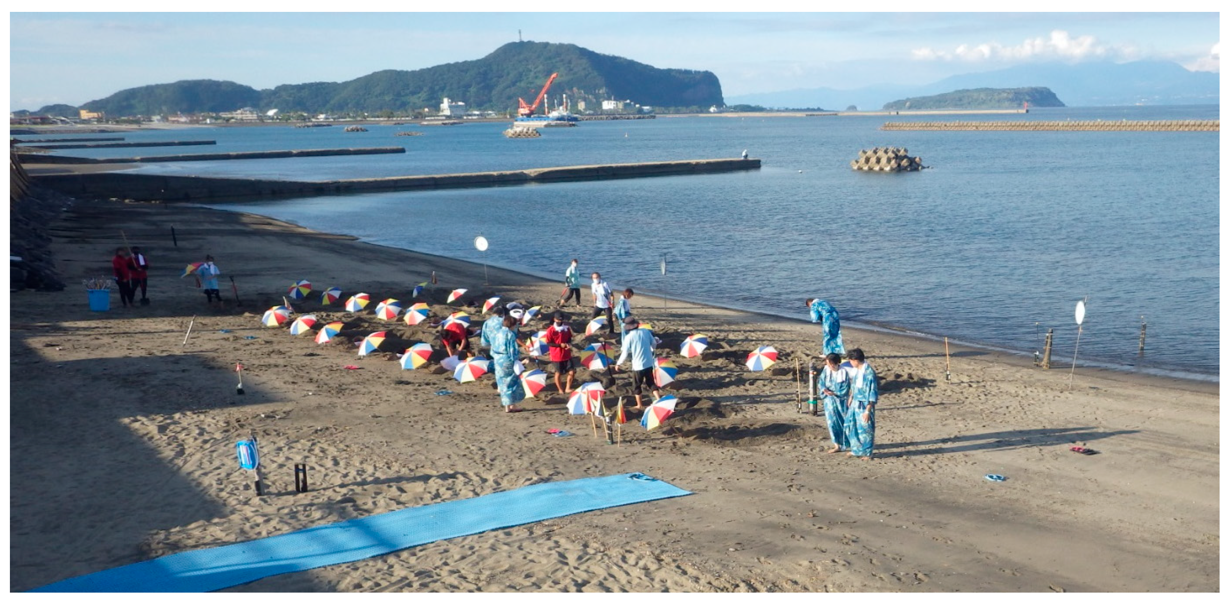
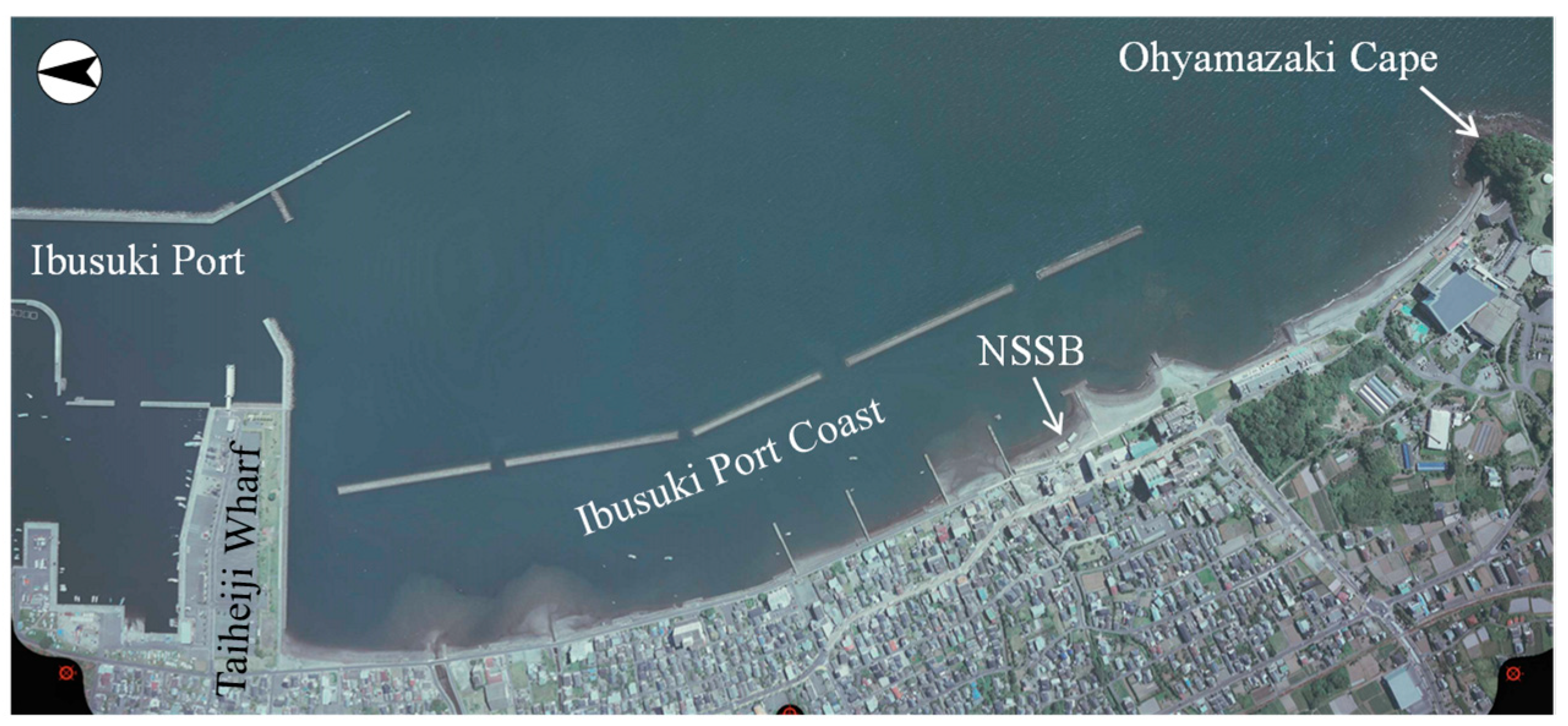
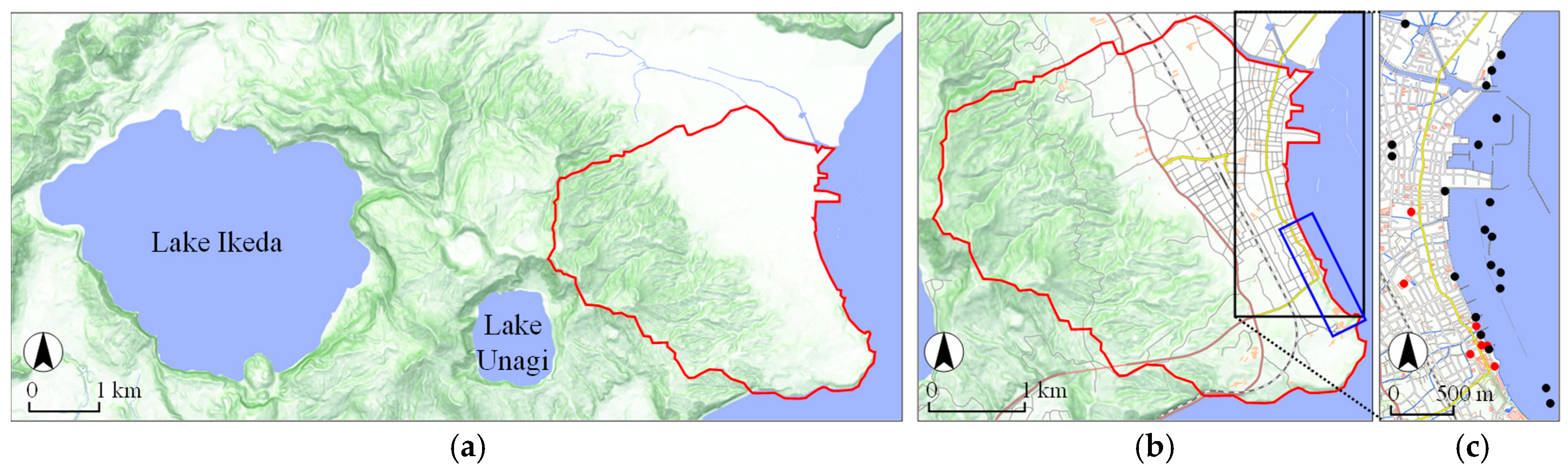
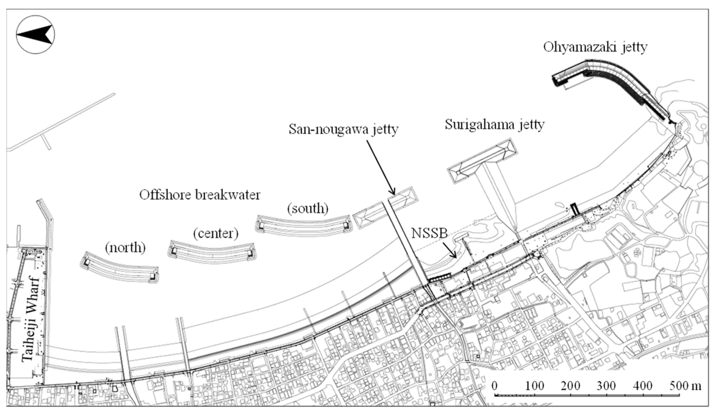
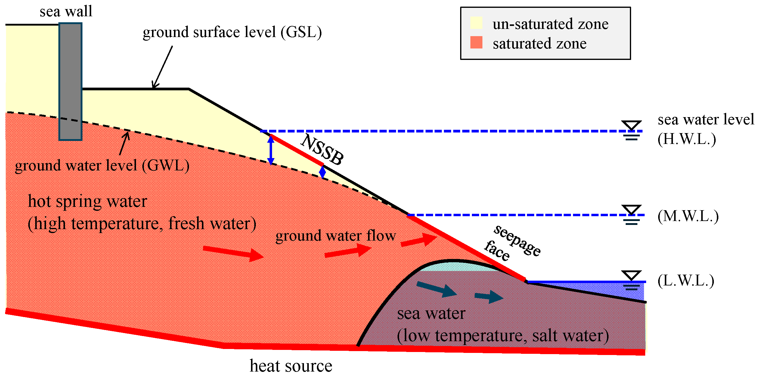
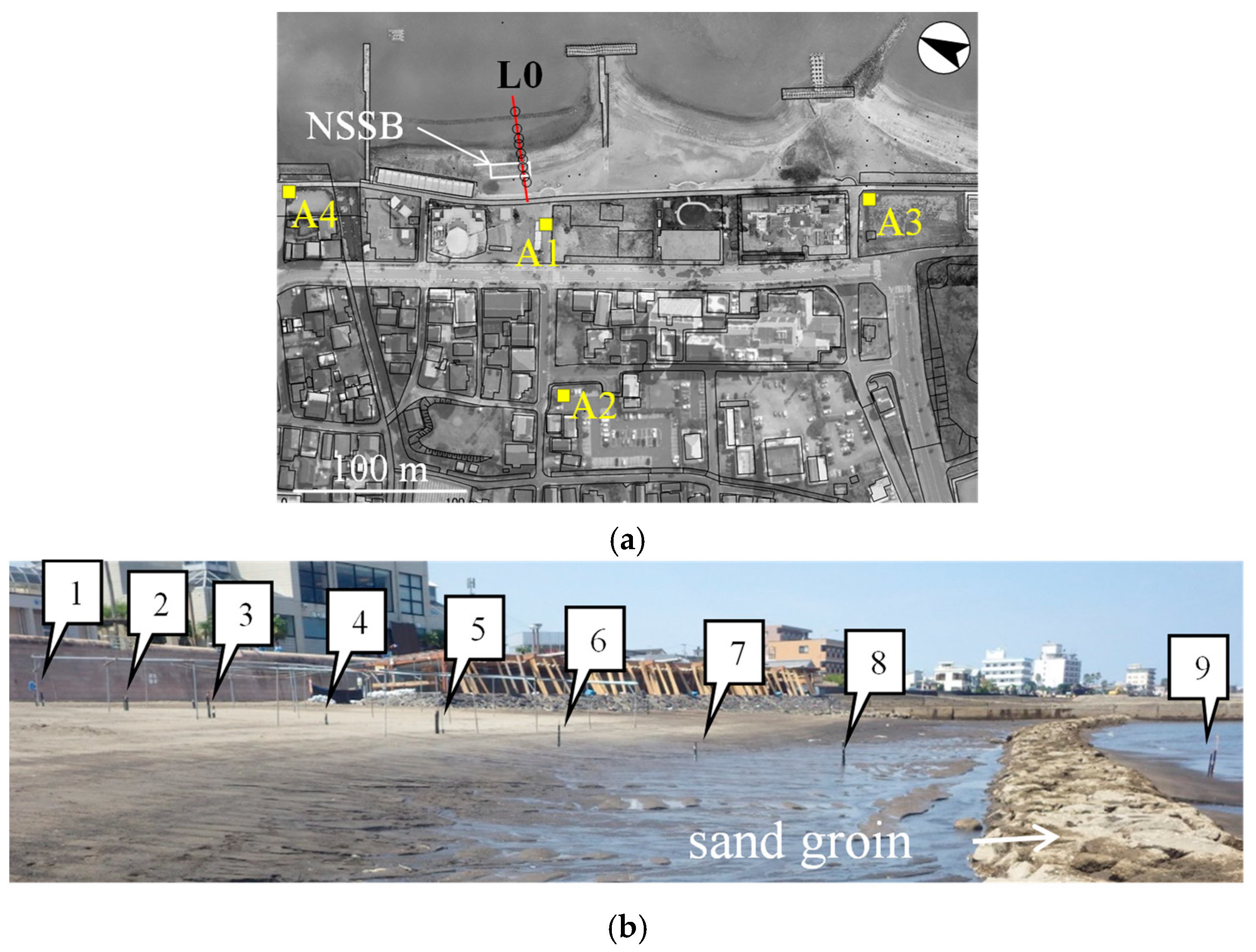
Groundwater dynamics in nearshore zones is one of the most important subjects in coastal engineering and water resource engineering, since it influences the nearshore hydrodynamics, beach morphodynamics, and groundwater use for irrigation. This subject has been studied over a long period of time and various findings have been established.

As early as the 1940s, studies were conducted on the dynamic properties of a beach water table in response to diurnal tidal motions. For example, Emery and Foster [1] and Grant [2] found that seepage streams generated on the foreshore surface create rill marks during low tide. The groundwater velocity is so small in comparison with the tidal velocity on a beach slope that the seepage point on the beach slope cannot follow the tidal level during an ebb tide. It results in a disconnection between the apex of the seepage face and the tidal water surface, which makes mathematical treatments difficult. Much later, Turner [3] proposed a simple model of the swashing motion on a sandy beach that focused on the process of water penetration into a sand layer.

The effects of swash zone infiltration/exfiltration processes were investigated from the perspective of sediment transport [4,5,6,7]. If we consider sediment transport on a beach under limited conditions, such as those that only account for tidal motion, or where wave motion is regarded as a small amplitude wave, swash motion can be regarded as sinusoidal, and the resulting net sediment transport during one tidal/wave period becomes null. However, even though the infiltration/exfiltration velocity is usually small, it contributes a non-negligible effect to swash sediment transport because the one-directional velocity compounds the sinusoidal velocity. The above studies were based on a saturated seepage flow model with a free surface in an unconfined aquifer. Ochi, Miyatake, and Kimura [8] investigated groundwater flow under swashing wave motion based on a saturated/unsaturated seepage flow model. They conducted a flow analysis by differentiating between a wetting process during a wave runup and a drainage process during a wave rundown on a slope.

Typically, the density of seawater is 2.0–3.5% greater than that of fresh water, which can cause seawater to intrude into a freshwater coastal aquifer. The saltwater wedge is one factor that complicates the physics in a coastal aquifer. Maintaining the freshwater resource in a groundwater aquifer is important for agricultural engineering, and previous studies have investigated the movement of the freshwater/saltwater interface. Although many earlier studies assumed an upright landform at the shoreline [9], Uchiyama [10] investigated groundwater flows under tidal motions, including the dynamics in the unsaturated zone, not only for an upright landform but also for a sloping landform. Subsequently, Uchiyama et al. [11] applied their model to describe the submarine groundwater discharge and the associated nutrient transport at a specific site.

As a study related to the coastal ground flow dynamics, the development of a soft shore protection method, i.e., the Beach Drainage System, should be quoted. This method enhances beach accretion by artificially lowering the groundwater table. In connection with the development of this method, numerical models to deal with coupling of the wave motion on a beach and the porous groundwater flow have been proposed (for review; Karambas and Ioannidis [12]). The effects of a beach drainage system on the evolution of the beach morphology have been studied in the field [13] and in a wave tank [14].

Recently, the role of the capillary fringe, which lies just below the sand surface, has attracted research interest, because it has influences on beach groundwater dynamics. Horn [15] stated that the presence of a capillary fringe can have a significant effect on the exchange of water between the ocean and the coastal aquifer. Hallin et al. [16] focused on the important role of the moisture content on the beach surface for aeolian transport. The surface moisture is closely related to the capillary rise coming from the groundwater table. A recent review on the current understandings and advances in groundwater dynamics in coastal unconfined aquifers was presented by Zheng et al. [17].

Existing coastal engineering studies, however, have not addressed the thermo-hydrodynamic groundwater flow problem with full-scale consideration. Groundwater motion in a hot spring geothermal region is driven by the gravity force caused by the water table gradient and by the buoyancy force caused by the temperature difference. At the study site, the fluid temperature can reach the boiling point of water. The density of water at 100 °C is 4.2% lower than that of water at 20 °C under standard atmospheric pressure. Deeper underground, as the pressure increases, the boiling point of water becomes higher than 100 °C. Allis and Yusa [18] presented a review of existing research on the geothermal system at Beppu, another well-known hot spring area in Japan. On a basis of comprehensive observations, they proposed a sectional diagram of the thermal distribution in which the maximum temperature reached 250 °C at a 600 m depth. Yusa [19] developed a mathematical model to describe the flow pattern and temperature distribution under a geological setting where the magnitude of depth was on the order of 1000 m. Many studies have reported on the hydrothermal characteristics of groundwater flows in various geological areas [20,21]. The governing factors of the flows vary a great deal, including the ground strata, fracture structure of the bedrock, geothermal supply system, and so on. Comparing the existing geothermal research to the present study, the water temperatures do not differ so much, although the former studies treat up to several hundred degrees. Significant differences are found for the spatial scale in the vertical direction, with the former being hundreds or thousands of meters, while this study focuses only several meters or tens of meters.

Numerical and experimental studies focused on thermal convection flows have been conducted from the perspective of thermal storage system development in areas where hot water stored in an aquifer is used for heating houses/buildings [22,23,24]. White et al. [25] developed a hydrothermal model to examine the application potency of a geothermal resource. In agriculture science, the mechanism of hydrothermal transport in an unsaturated zone is also an important subject. Deb et al. [26] investigated temporal variations in the water content and soil temperature in a sandy loam-irrigated field by using a water–vapor–heat transport-coupling numerical model. However, the temperatures they were concerned with covered a small range from approximately 10 °C to 30 °C.

As described above, analyses of groundwater flow, including heat transfer, have been undertaken previously for various purposes; however, the spatiotemporal scales of the phenomena, along with its physical properties, boundary conditions, and heat transport forms, differ widely and most are markedly different from those found at the Ibusuki Port Coast site. Therefore, we conclude that relevant knowledge that is directly applicable to our study site is lacking.

2. Study Site

The location of the Ibusuki Port coast, where this study was conducted, is already shown in Figure 1. The topography and geography of the entire area of southern Kyushu strongly reflects the substantial volcanic action that occurred during the late Pleistocene and Holocene epochs. One of the primary geological features in this area is the volcanic deposits that were generated, namely Shirasu, which is one of the dominant widespread and thick regional deposits [27]. A huge eruption that occurred 110 thousand years ago generated a large caldera (the Ata caldera), and the Ibusuki area is on the northwestern edge of this caldera. The most recent huge eruption occurred 5500 years ago. The current regional geography is characterized by the craters and subsided landform structures generated, such as Lake Ikeda and Lake Unagi (Figure 4). The New Energy and industrial technology Development Organization of Japan (NEDO) reported that there remains a volcanic heat source in the deep underground area with sporadic uprising flows of high-temperature fluid. Geothermal observations suggest that there could be several reservoirs of high-temperature fluid under the highlands in the Lake Unagi area. Therefore, it has been conjectured that these geothermal reservoirs could be the source of the Ibusuki hot spring, but knowledge regarding the existence of the channels supplying hot water from the reservoirs to the NSSB area remains uncertain.

Figure 5 illustrates the objective of the coastal improvement project in the Ibusuki Port Coast area. It can be seen that a curved sandy beach that extends for over 1.8 km is bounded by the Taiheiji wharf at the northern end and by the Ohyamazaki jetty at the southern end. The observations and numerical analyses in this study focused on the coastal zone surrounding the NSSB area. Figure 6 conceptualizes the flow mechanisms involved in coastal groundwater flow under the influence of both water temperature variations and tidal level fluctuations.

To determine the viable conditions for the NSSB, we undertook a verbal question-and-answer survey with the staff engaged with the service on a daily basis, and we conducted supplemental observations to verify the survey results. It was established that the surface temperature must be approximately 60–80 °C. The most feasible time for an NSSB is when the tide is at its lowest and during the 3 h following the spring tide. The optimal bathing site is where the ground surface level (GSL) is between the mean and high water levels at the spring tide, as shown in Figure 6. These conditions imply that the surface sand layer must be dry. During the period of unsuitable conditions, tidal water floods the bathing site and penetrates the surface sand; consequently, the surface sand becomes saturated.

According to an experimental study on low-temperature burns [28], the occurrence of a cutaneous injury is determined by the surface temperature of a heat source and the exposure period. For example, a burn injury can occur with an exposure of 2 min (several seconds) at a surface temperature of 50 °C (60 °C). However, bathers at the NSSB site are often content to remain buried in the hot sand layer for several or tens of minutes. The reason why this is feasible without injury reflects the dry status of the sand and the entrapment of air in the surface sand layer. In the NSSB experience, an attendant excavates a small trench (depth: approximately 10 cm) on the beach, the process of which introduces air into the dug sand. Then, a sand bather lies on their back in the trench and the attendant covers them (except for their head) with the dug sand. The heat capacity of air, evaluated as the product of the specific heat and density, is only 1/4000 that of water. If the surface sand layer contains sufficient air, a sand bather will not suffer a heat-related injury because their body is in contact with a thin layer of the air–sand mixture that is subject to rapid cooling.

Although the dry condition of the surface sand layer is a requirement for sand bathing, if the GSL is far from the hot groundwater, the bathers will not experience sufficient warmth. The index of viability for sand bathing can be described by the distance between the GSL and the groundwater level (GWL). Consequently, knowledge of both the temperature and the water content ratio (dryness) of the surface sand layer is necessary to describe the conditions suitable for the NSSB experience. To determine the appropriateness of beach nourishment work, the viable conditions for sand bathing should be quantified. From the above considerations, the relevant conditions are as follows: the feasible period extends for 3 h from the time of low tide, the feasible depth is approximately 0.2 m below the GSL, the average feasible temperature at that depth is 65–80 °C, and the GSL–GWL distance is 0.3–0.6 m.

3. Materials and Methods

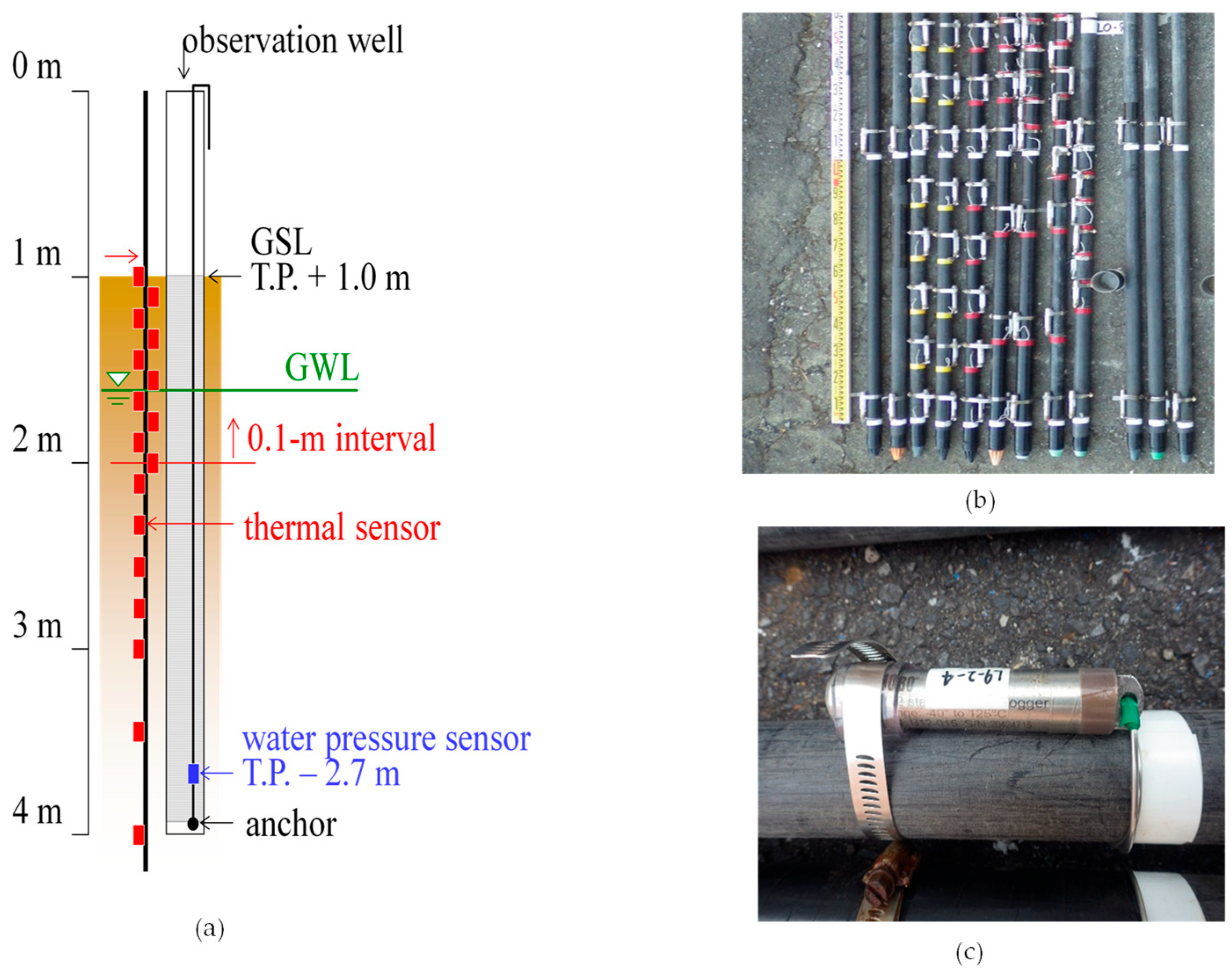
3.1. Field Observations

3.1.1. Overview of the Observations

Field observations were conducted at the Ibusuki Port Coast site over 7 years (2016–2022). In the early stage, observations were made to elucidate the general characteristics of the thermo-hydrodynamic environment of the entire area. As the project proceeded, the observations became focused on the NSSB area; that is, measurements of the spatiotemporal variations in the GWL and the temperature in the sand layer (TISL). The beach bed at the study site is composed of three phases: solid particles (mainly sand), fluid (water), and air. The thermal field in this area is governed mainly by heat conduction among these three phases. Heat conductivity is affected by several factors such as the specific thermal conductivity of each phase, water content ratio, and air void ratio. Thus, the temperature that we measured, or tried to reproduce via numerical analyses, i.e., the TISL, reflected the aggregate three-phase temperature of the soil–water–air mixture.

We started our observational campaign by collecting basic data. A survey of the grain size distribution in the NSSB area revealed that the largest proportion of the deposits is sand (91.1%), with the remaining fractions consisting of gravel (8.2%) and silt (0.7%). The 50% and 20% grain diameters (i.e., d₅₀ and d₂₀, respectively) were estimated at 0.50 and 0.33 mm, respectively. The grains prepared for use in the beach nourishment work comprised 76.6% sand, 4.6% gravel, and 18.8% silt, and the representative d₅₀ and d₂₀ values were 0.41 and 0.11 mm, respectively. The estimated hydraulic conductibility (k) based on the d₂₀ value was 2.72 × 10⁻² cm/s for the sand in NSSB area, and 1.94 × 10⁻³ cm/s for the sand used in the beach nourishment work.

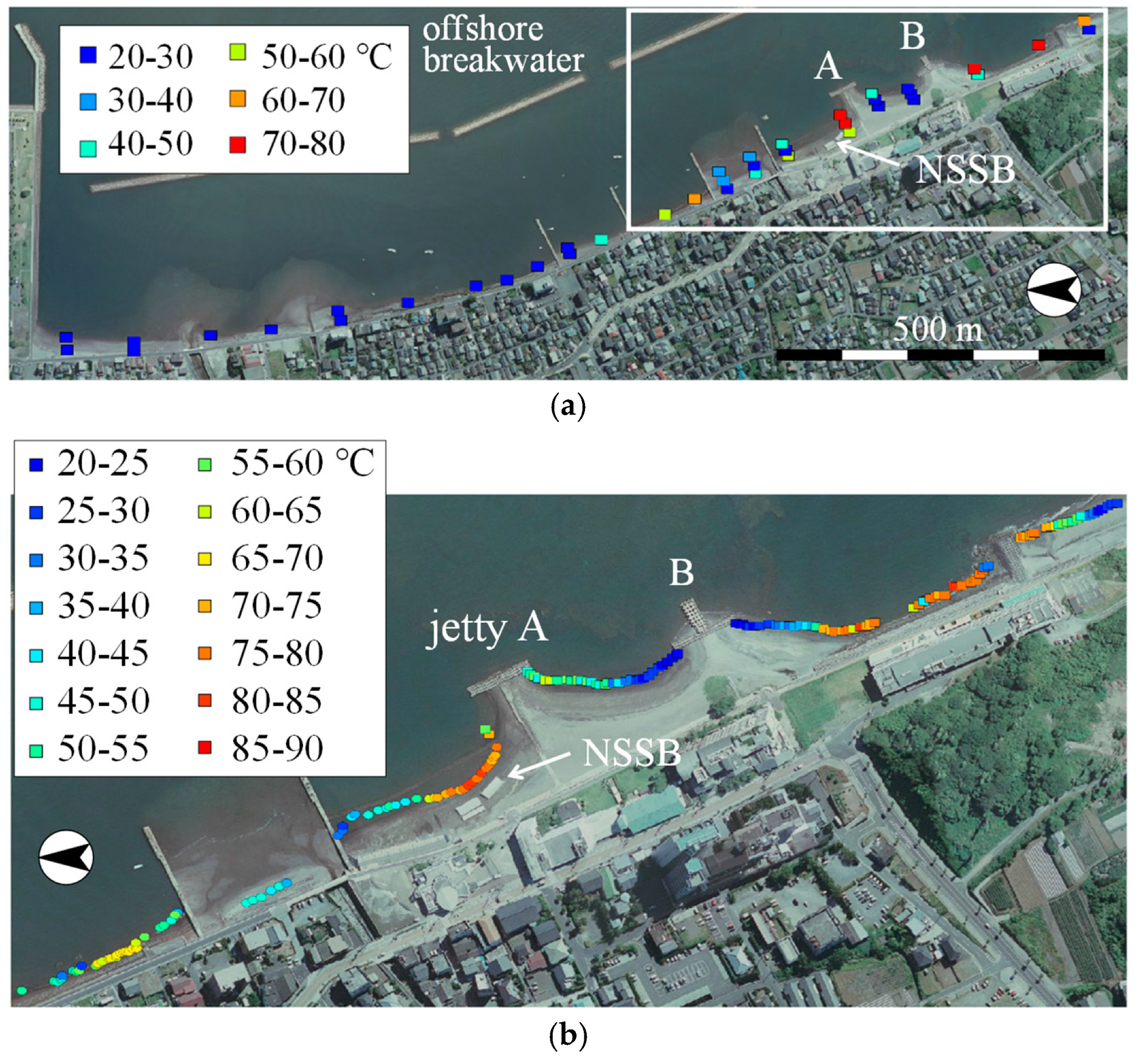
3.1.2. Alongshore Measurements

Figure 7 shows thermal images of discharging hot spring water during an ebb tide taken using an infrared thermographic camera. Because the temperature of the beach surface is affected by solar radiation during daytime, these photos were taken at night. The white dotted line in each photo indicates the shoreline position. It is evident from the photos that hot spring water exudes just above the shoreline as the ebb tide process becomes advanced.

The above result indicates that the water temperature seeping out near the shoreline is strongly governed by the tidal level. To investigate the thermal conditions along the entire coast, it is necessary to complete the observation within a short period of time when the tidal level can be regarded as almost constant. Alongshore temperature measurements along the shoreline were conducted between 2016 and 2017. During the low tide period at spring tide, we tried to simultaneously measure TISL at a depth of 0.5 m from the sand surface by deploying 6~7 staff members. The measurements were practically completed within one hour.

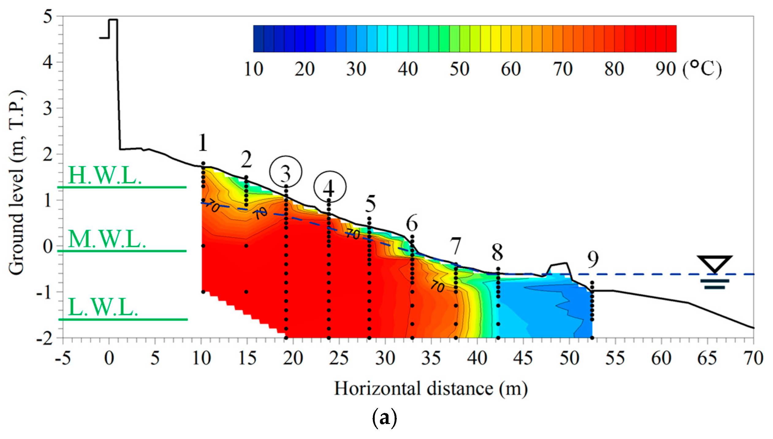
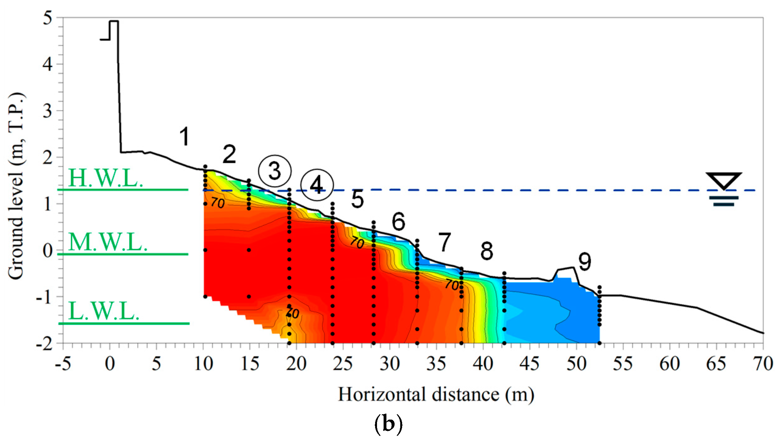
3.1.3. Cross-Sectional Measurements Along the NSSB Transect

Detailed measurements of the GWL and TISL were conducted along survey line “L0” in the NSSB area (Figure 8). Measuring stations, denoted as St.-1 to St.-9, were set in the cross-shore direction from the sea wall to beyond the sand groin at 5 m intervals. At each station, measuring points for the TISL were taken in the vertical direction at 0.1 m intervals from the ground surface to the depth of 1.0 m, and then at coarser intervals in the deeper region. The total number of TISL measuring points was >150. At St.-1, St.-3, and St.-5, the GWL was also measured with water pressure sensors. Furthermore, the GWL and hot spring water temperatures were measured by boring surveys conducted at points A1, A3, and A4 behind the sea wall and at point A2 within the residential area (Figure 8a). Tidal level fluctuations at Ibusuki Port were also measured during the observation period.

To measure the GWL, observation wells were drilled using heat-resistant PVC pipes with outer diameter of 76 mm (Figure 9a). The deployment of the measuring devices in the observation wells is also shown in the figure. The pipes were driven as far as 4 m into the beach using a water jet method. To allow the groundwater to enter the pipes, 0.5 mm wide slit holes were opened around the circumference of the pipe. The total opening ratio was 10%, and nonwoven fabric was attached to the outer pipe to prevent ingress of fine grained sand. The water level gauge used was a durable high-temperature air bubble water level gauge (Bubble Card2; Meteo Electronics Co., Sapporo, Japan). The gauge was suspended from the top of the observation well on a rope, and its elevation was measured using a stainless-steel measuring tape fixed to the rope. Complementary measurements using a rope-type water level gauge (WL-50, Type 3; Alpha Kougaku Co., Kyoto, Japan) were also conducted to ensure measurement accuracy. As noted above, the objective was to measure the TISL. Therefore, thermometers (HOBO U12; Onset Co., Bourne, MA, USA) were installed on the outside of the fiber reinforced plastic (FRP) pole at 10 cm intervals to measure the TISL (Figure 9b,c). The thermometers were mounted alternately on the front and rear surfaces of the pole to prevent sensor-to-sensor heat transfer.

3.2. Numerical Analysis

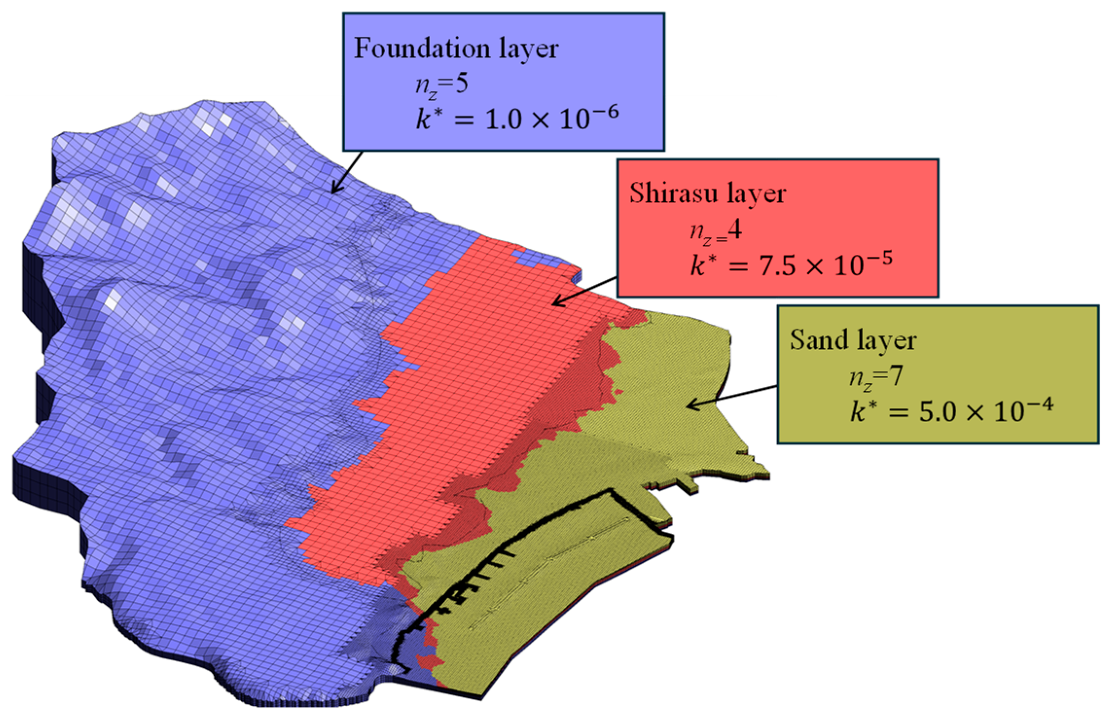
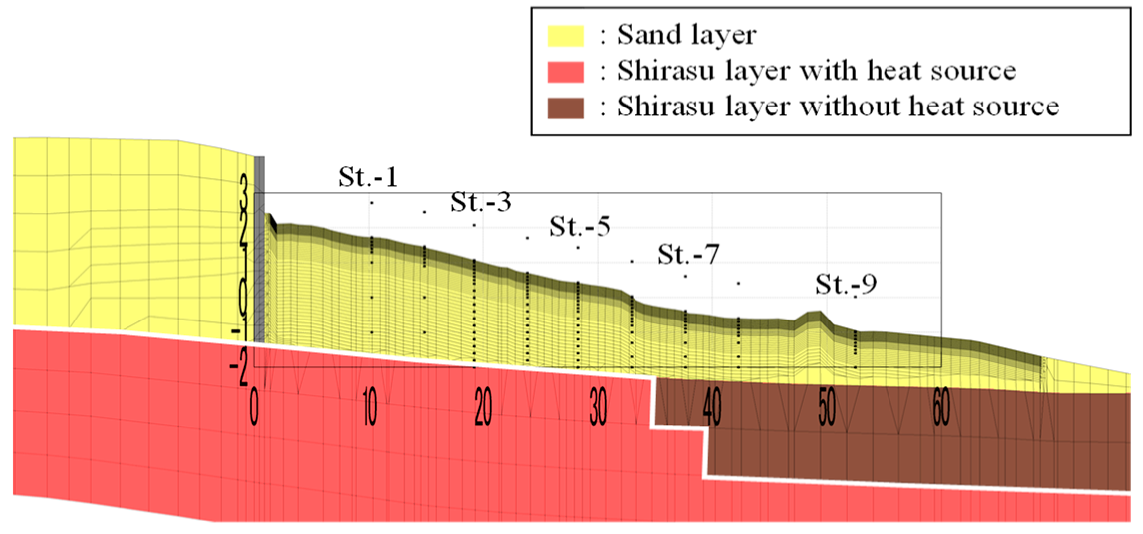
3.2.1. Computational Domain

A nesting grid system comprising three computational domains was employed for the numerical analysis (Figure 10). On the basis of the topographic characteristics of the Ibusuki area shown in Figure 4, the broad domain was set to fit the boundaries of the watersheds and rivers. The narrow domain was set to analyze the hot spring groundwater in the NSSB area in detail. An intermediate domain was provided to connect the broad and narrow domains. The maximum horizontal grid size in the broad domain was approximately 50 m on the mountain side. The grid size in the narrow domain varied from a maximum of 10 m to a minimum of 0.5 m.

Earlier boring surveys conducted at this site indicated that the vertical structure is generally stratified from the bottom to the surface with three layers: the foundation layer, the Shirasu layer, and the sand layer. The number of vertical grids was set with reference to this geological property. The hydraulic conductivity for each layer was given as a representative value by referring to the average diameter of the particles composing the layer. For detailed analysis of the groundwater flow in the NSSB section, a high-density grid system was employed to resolve the near-ground surface flows with high accuracy (as discussed in Section 5.1).

3.2.2. Boundary Conditions

The landward boundary condition of the GWL in the narrow domain was given by the steady-state computed results of the intermediate domain. The seaward boundary condition was given by the time-varying tidal level fluctuations. In the heat transport analysis, the temperature of the groundwater at the landward boundary was set at 85 °C. Along the subaerial/submerged ground surfaces, the average air/seawater temperatures during the observation period were set. As a bottom boundary condition, a temperature of 95 °C was applied at the interface between the shallower sand layer and the deeper Shirasu layer. Under the above boundary conditions, a 150-day run-up computation was implemented, and the subsequent results were adopted based on the assumption that transient distortions of the initial settings were fully attenuated.

3.2.3. Basic Equations

The present numerical analysis is based on Dtransu-3D EL model developed by Nishigaki et al. [29]. The model name, “Dtrans-3D EL”, stands for letter abbreviations of “Density-dependent TRANSport analysis Saturated–Unsaturated porous media—3 Dimensional Eulerian Lagrangian”. As the name indicates, the model possesses capabilities to simulate coupled saturated/unsaturated seepage flow analyses, solute transport, and advection–dispersion analyses. Since the model structure is based on the finite element method using an unstructured grid system, it is versatile and can apply detailed configurations of topography and geological structures in terrestrial area.

We developed a groundwater model by including consideration of heat transfer system to the Dtransu-3D groundwater model. The governing equation for the groundwater flow is as follows:

$${\displaystyle \frac{\mathcal{\partial }}{\mathcal{\partial }{x}_i}}\left(\rho K_r{K}_{ij}^S{\displaystyle \frac{\mathcal{\partial }\phi }{\mathcal{\partial }{x}_j}}+\rho K_r{K}_{i3}^S\right)+\rho q=\rho \left(\beta S_s+C_s\right){\displaystyle \frac{\mathcal{\partial }\phi }{\mathcal{\partial }t}}$$

(1)

where i, j, and i3 are a summation-convention expression for the x-, y-, and z-direction components, respectively; ρ is fluid density (kg/m³); K_r is the specific conductivity; $K^S$ is the saturated conductivity (m/s); $\phi$ is the pressure head (m); $\beta$ is the effective index (set to 1 and 0 for the saturated and unsaturated state, respectively); $S_s$ is the specific storage coefficient; and $C_s$ is the specific water capacity. The value of $K^S$ for each domain shown in Figure 10 was set with reference to the in situ observations of the particle diameter distributions.

For the heat transport analysis, we considered a heat transfer process at the surface boundary between the sand layer and the air/seawater in addition to the advection–diffusion process presented by the Dtransu model. Including the process in the third term of the right hand side, the governing equation for heat transport is expressed as follows:

$$\theta {\displaystyle \frac{\mathcal{\partial }T}{\mathcal{\partial }t}}={\displaystyle \frac{\mathcal{\partial }}{\mathcal{\partial }{x}_i}}\left(\theta D_{ij}{\displaystyle \frac{\mathcal{\partial }T}{\mathcal{\partial }{x}_j}}\right)-\theta V_i{\displaystyle \frac{\mathcal{\partial }T}{\mathcal{\partial }{x}_i}}-{\displaystyle \frac{1}{\rho c_f}}{H}_L(T-T_r)$$

(2)

where θ is the volumetric water content, T is the TISL (K), $D_{ij}$ is the dispersion tensor, $V_i$ is the groundwater flow velocity (m/s), $c_f$ is the groundwater specific heat (J/kg/K), $H_L$ is the heat transfer coefficient (W/m³/K), and $T_{r }$ is the temperature of the atmosphere or seawater (K) in contact with the ground surface. The dispersion tensor $D_{ij}$ is described as a function with the following variables: longitudinal and transverse dispersion length α_L and α_T, groundwater flow velocity components perpendicular and along the plane of a computational cubic cell, and thermal diffusion coefficient $D_{\mathrm{d}\mathrm{i}\mathrm{f}\mathrm{f}}$. The specific values for the above parameters used in this study are summarized in

Table 1. Setting values for heat transport analysis.

Coefficient	Value
	Foundation Layer	Shirasu Layer	Sand Layer
Effective Porosity $n$ (-)	0.100	0.100	0.393
Specific storage coefficient $S_s ($m−1)	1.0 × 10−5	1.0 × 10−5	1.0 × 10−5
Thermal diffusion coefficient $D_{\mathrm{d}\mathrm{i}\mathrm{f}\mathrm{f}} ($m2/s)	1.0 × 10−6	1.0 × 10−6	1.0 × 10−6
Longitudinal dispersion length ${\alpha }_L$ (m)	5.0	5.0	5.0
Transverse dispersion length ${\alpha }_T ($m)	2.5	2.5	2.5

. The heat transfer coefficient $H_L$ represents the heat exchange efficiency between a heated body and the surrounding fluid. The coefficient is regarded as not a physical property value, but a state-dependent value. In this study, after trial calculations to reproduce the observed temperature results, the best fitting value for $H_L$ was determined to be 1000 W/m³/K for the interface between the beach surface and the atmosphere, and for the interface between the beach surface and the seawater.

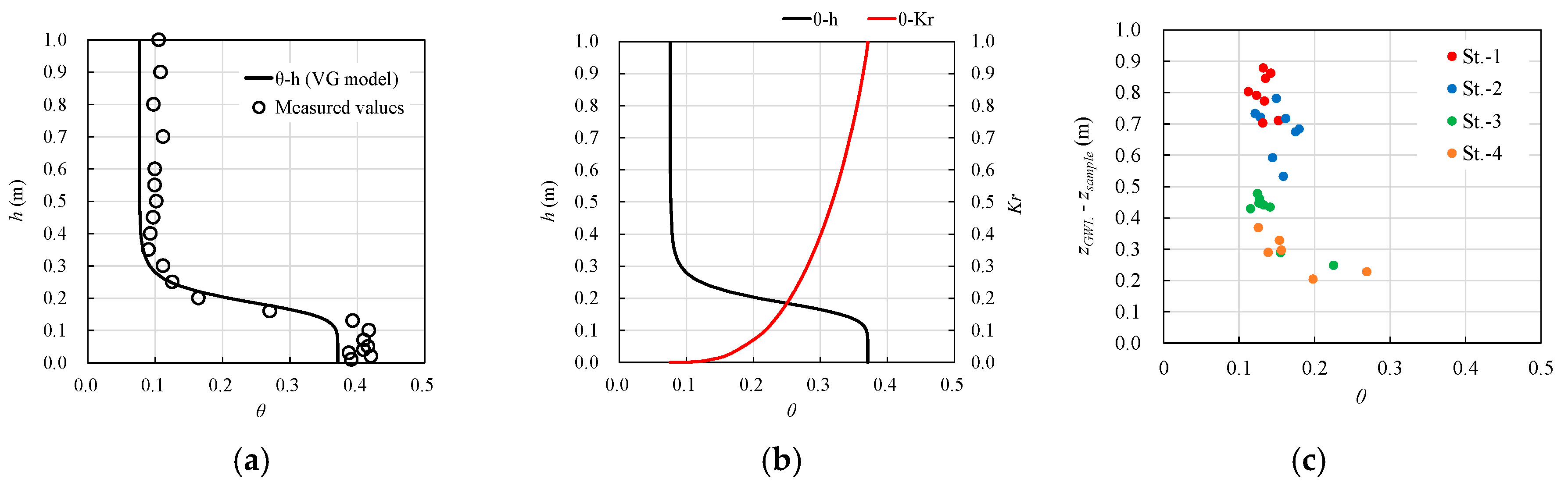
3.2.4. Saturation/Unsaturation Characteristics

Regarding the NSSB feasibility conditions, the volumetric water content in the surface sand layer is an important factor. As a preliminary study, we intended to confirm whether the observed water retention characteristics in the sand layers sufficiently reproduce the established theory on the hydraulic conductibility of unsaturated sand layers. Then, the results obtained were incorporated into the parameter setting in the numerical analysis.

We conducted laboratory experiments to examine the relationship between the volumetric water content $\theta$ and the suction head h in sand layers near the ground surface. Taking sand column samples where NSSB is implemented, we brought the samples to a laboratory and measured $\theta$ and h, employing sand column method [30]. The value of θ was evaluated by vaporizing the interstitial water and using the SWRC fitting method [31]. From the established relationship between $\theta$ and h, the best-fitted parameters involved in VG model proposed by van Genuchten [32] were determined.

Figure 11a illustrates results measured in the laboratory on the relationship between $\theta$ and h, whereas Figure 11b shows the corresponding relationship based on VG model. The results obtained were found to fit well with the curve of VG model. Consequently, we have obtained the proper characteristic curve for the water contents, and it can be applicable to the present numerical analysis on thermo-hydrodynamics with sound observational basis. It was also found that the volumetric water content ration θ reaches the minimum water content θ = 0.1 under the condition that h is greater than 0.3 m. Note that this is consistent with the feasible conditions for NSSB clarified in Section 3, as the distance from GSL to GWL is 0.3–0.6 m.

We conducted field measurements on the volumetric water content θ by sampling specimens at various depths along the L0 transect during the flood tide period. Figure 11c shows the relationship between θ and the vertical distance of the sampling point z_sample from GWL. Since the maximum possible value of the water content is approximately 0.3, the result indicates that the sand layer is saturated up to a height of 0.1 m above the GWL. In the upper region from 0.1 m, the volumetric water content was found to decrease rapidly. It was also observed that when the vertical distance from the GWL (z_GWL-z_sample) becomes >0.3 m, θ becomes almost constant at approximately 0.15. The general tendency shown in Figure 11c broadly agrees with the moisture characteristic curve shown in Figure 11a, and supports a feasible condition for NSSB where the distance from GSL to GWL is within a range of 0.3–0.6 m.

4. Results

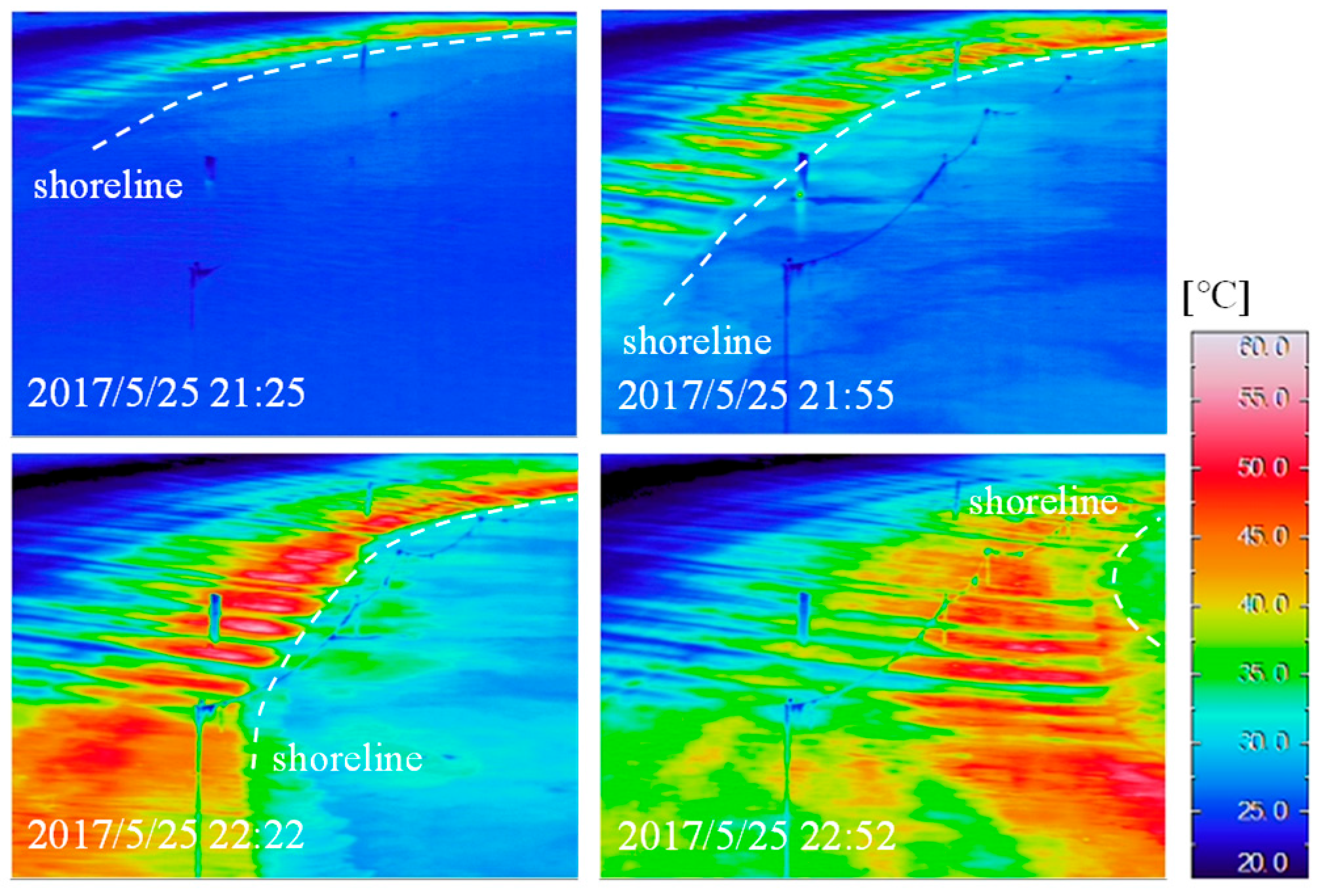
4.1. Observational Results

Figure 12a presents the results for the entire area, and Figure 12b shows the results around the NSSB zone in greater detail. Areas with temperatures reaching up to 70 °C were observed in the NSSB zone and to the south of point B, shown in Figure 12b, but the extent of these areas was restricted, and even between these hot areas, a zone with low temperatures of approximately 30 °C was found. These results suggest that the thermal structure of the coastal groundwater is not uniform in the alongshore direction, and that the hot spring water exudes only in specific spots.

Figure 13 shows the cross-sectional distributions of the TISL and the profiles of the GWL along the L0 transect at low tide (Figure 13a) and at high tide (Figure 13b) during a spring tide cycle. The solid black line indicates the GSL, and the dashed blue line depicts the position of the GWL.

Notably, the GWL at St.-1 is at approximately T.P. (Tokyo Peil) + 1.0 m, and the GWL at the shoreline, approximately 30 m horizontally from St.-1, is at T.P. −0.5 m. Therefore, the hydraulic gradient of the groundwater flow was estimated to be approximately 1/20 at low tide. The following properties can be determined from Figure 13a: near St.-3 and St.-4, where the sand bathing is performed, the GSL–GWL difference is approximately 0.3–0.6 m, and the surface sand temperature is approximately 65 °C, consistent with the NSSB feasibility conditions discussed in Section 3. Figure 13b shows that the surface sand temperature at high tide is cooled over a wide range. The temperatures at St.-8 and St.-9 in Figure 13a,b are remarkably low compared with those at other stations. One possible cause may be seawater intrusion into the aquifer. However, the interface of the hot and cool TISL does not show a wedge-like feature; instead, it is broadly uniform from the surface to deeper inside. We conducted observations in 2021 along the L0 transect, which revealed the same characteristics as found in the 2022 observations. Therefore, this characteristic is not considered to be caused by observational failures.

Thus, it can be inferred that the position of the heat source on the offshore side suddenly becomes deeper than that on the landward side, i.e., at St.-1 to St.-7. Note that the location and the profile of the sudden temperature change around St-8 remains almost the same between low tide and high tide. This also suggests that the heat source might sink down in this area. The distributions of the water temperatures collected at the shoreline positions shown in Figure 12 also indicate the existence of spot-like high-temperature zones. Taken together, it can be deduced that such distinctive features result from localized heat sources in the underlayer. In Figure 13, the cooling effect of the low-temperature seawater infiltrating from the upper part of the beach during the rising tide is scarcely observed beyond the surface layer. Since low-temperature seawater has a higher density, the seawater infiltrating from the beach may sink to deeper areas due to the convection caused by the density differences with the hot spring groundwater flowing from the landward side. However, as standard salinometers are effective only at temperatures below 60 °C, it is difficult to measure salinity under high-temperature conditions, and thus the presence of saltwater intrusion into deeper areas beyond the observed range in this study has not been confirmed.

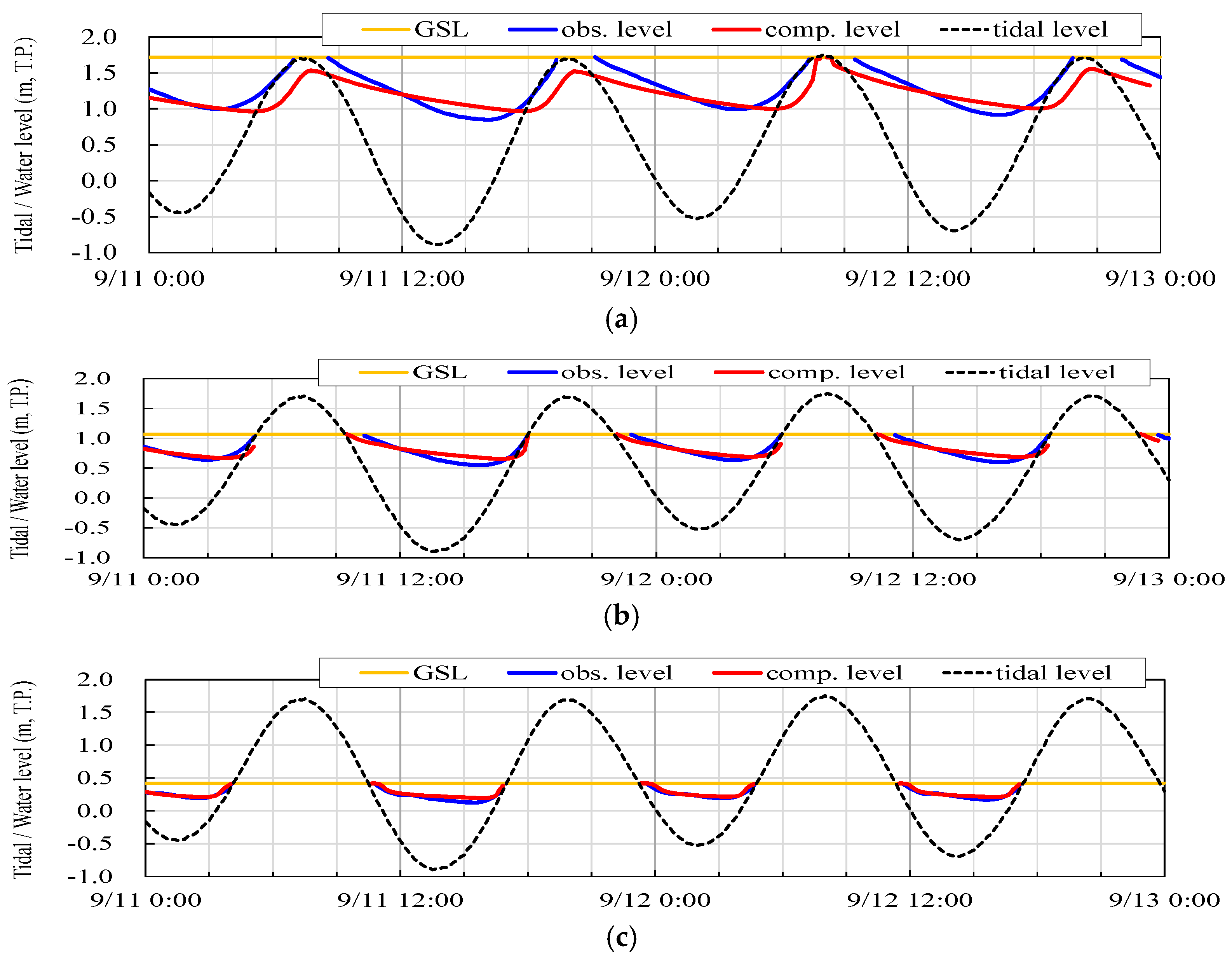
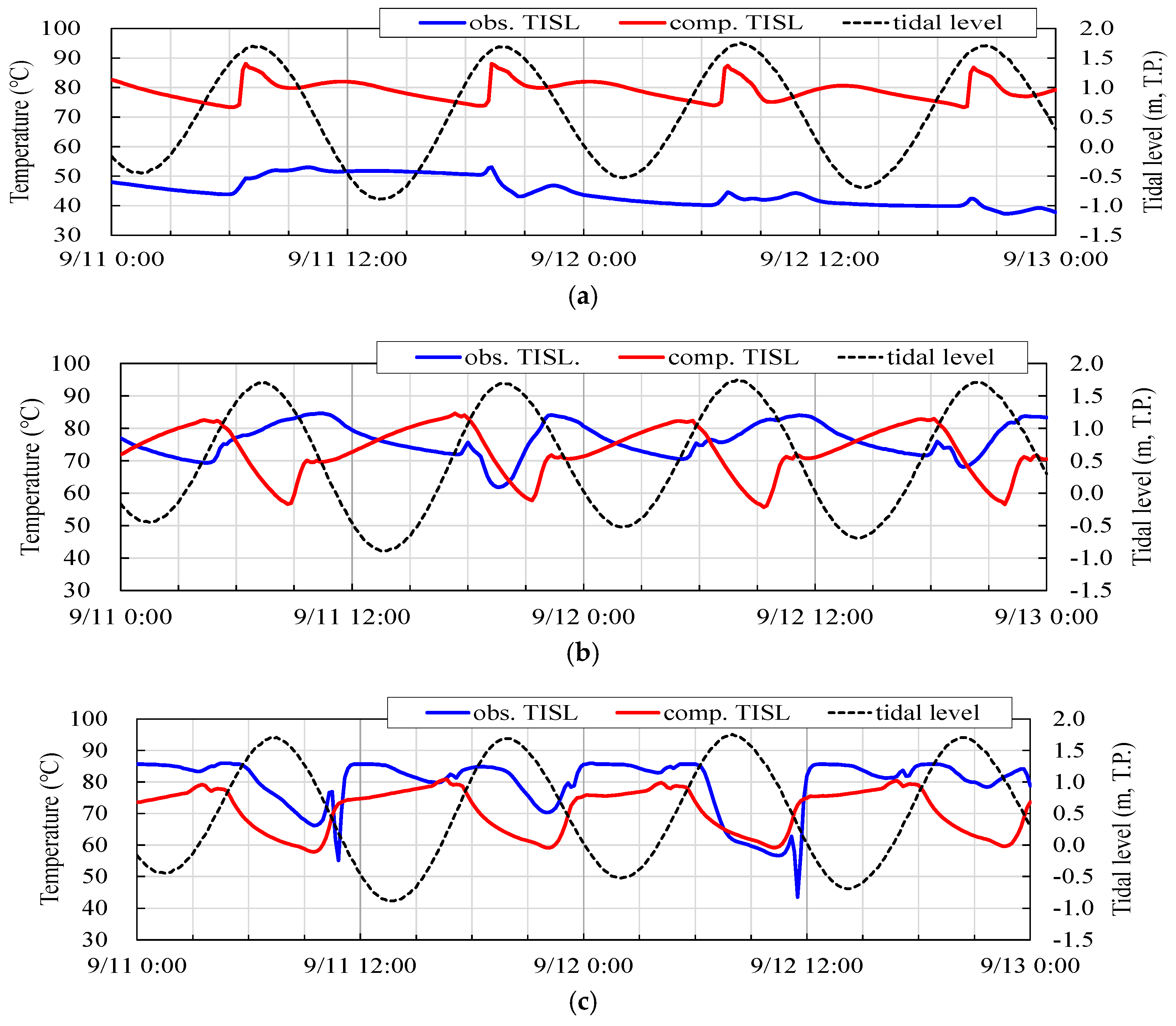
4.2. Computational Results

Focusing on the L0 transect where sand bathing is performed, the reproducibility of the present analyses for the observation results was examined. As shown in Figure 13, the low-temperature zone found in the observation results expanded offshore from St.-8, regardless of the tide level. The cause of such a characteristic could be attributed to the local nonuniformity of the heat source. However, accurate measuring of the heat source distribution is almost impossible because of the limitations of the measuring devices used under deep and high-temperature conditions. Therefore, in this analysis, to reproduce the high-temperature area landward from St.-7 and the low-temperature area offshore from St.-8, an adjustment was made by lowering the heat source depth by approximately 3 m in the offshore area, as shown in Figure 14.

Figure 15 illustrates the computed results of the TISL in the same form as the observed results shown in Figure 13. After an adjustment of the heat source depth, the computed results were found to adequately reproduce the observations throughout the entire area. Other computational results will be shown in the next section, where a comparative discussion with the observation results will be presented.

5. Discussion

5.1. Assessment of Reproducibility of Groundwater Table and Sand Temperature

The GWL and TISL are temporal changing properties that reflect tidal level fluctuations, which specify their offshore boundary conditions. The time series properties of both quantities were examined at three stations: St.-3, where sand bathing is performed, St.-1, at the most landward point, and St.-5, at the seaward point.

Figure 16 shows the observed and computed GWL fluctuations for comparison. The reasonable agreement between the computed and observed GWL time series confirms the reproducibility of the numerical analysis regarding GWL fluctuations. Figure 17 compares the observed and computed TISL at a depth of 0.2 m from the GSL. The result at St.-3 shows that the computed TISL fits with the observed TISL as time-averaged values; however, discrepancies are evident in terms of phase variations. The results at the landward point St.-1, where the unsaturated layer at the surface is thick, show that the averaged computed value is markedly higher than the observed value. The results at the seaward point St.-5 also indicate certain differences in terms of both the averaged value and the phase variation.

There are several possible reasons for the insufficient reproduction of the time-varying temperature near the sand surface. For example, the VG model does not fully reflect the moisture characteristics in the saturated and unsaturated regions, the effect of the moisture is not taken into account in the heat loss coefficient of the sand surface, and the effect of the density differences due to the temperature and salinity in the seawater infiltration from the sand surface is not taken into account. Because the time-varying surface temperature is a phenomenon in which the heat loss at the sand surface, the saturated and unsaturated infiltration flow in the sand layer, and the temperature and salinity are intricately related, it was difficult to completely reproduce the temperature change pattern, which varies greatly even with slight differences in location. In summary, the present numerical analysis does not adequately reproduce the time-dependent heat transport process that occurs near the ground surface. This suggests that a reliable prediction of the TISL after the beach nourishment work would be difficult under this complex thermal source condition.

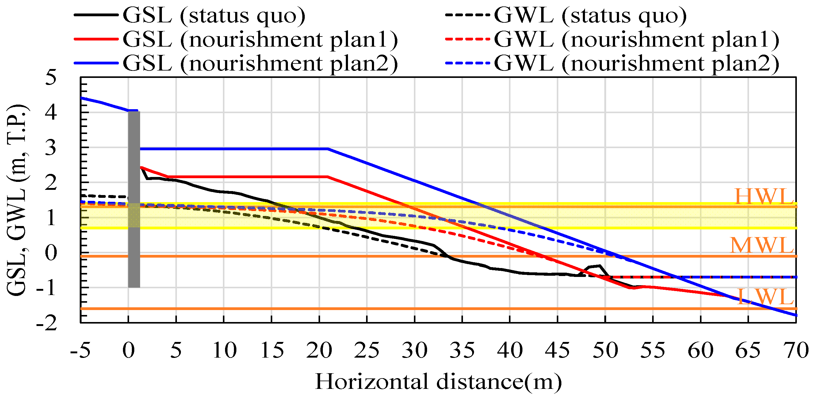
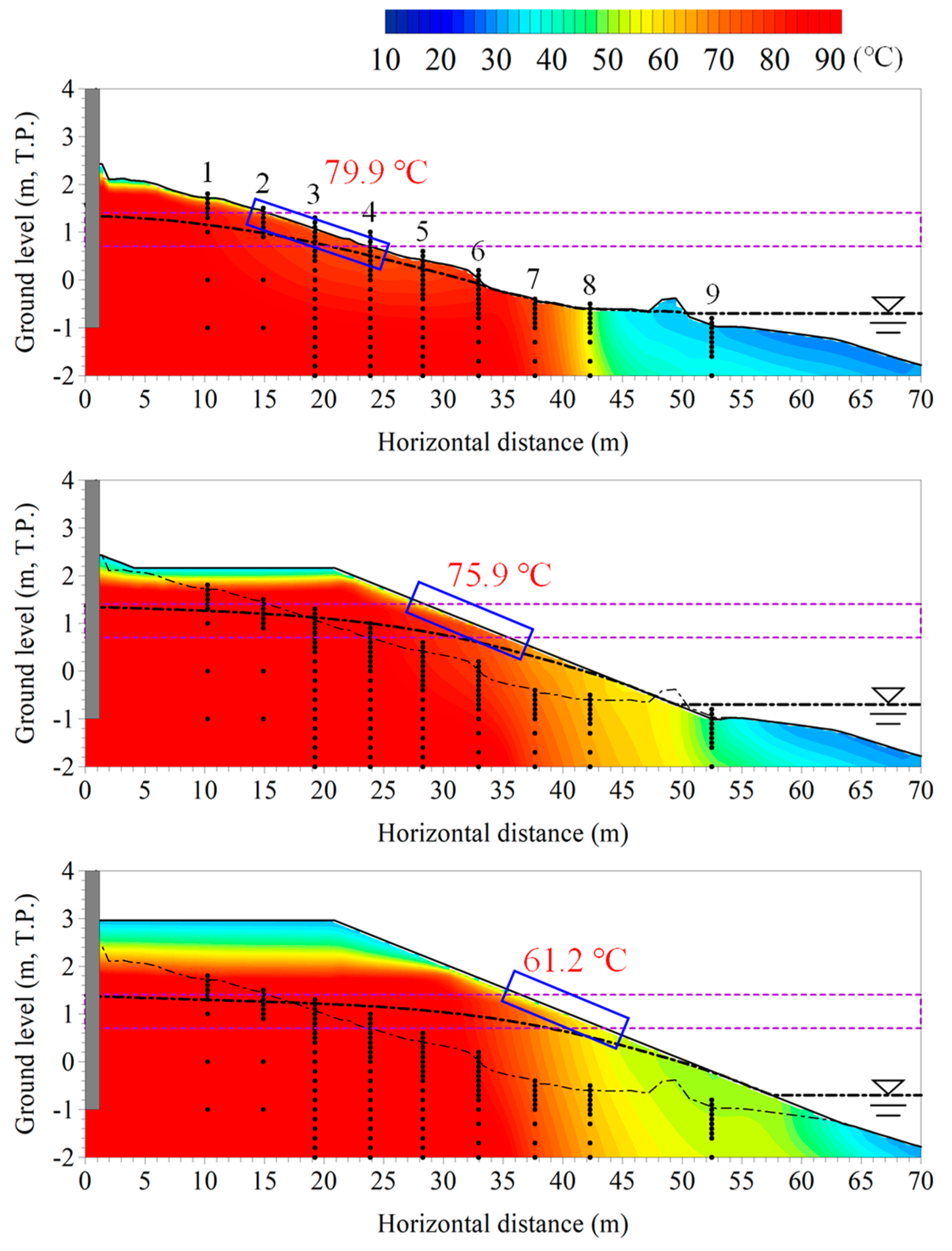
5.2. Impact Assessment of Beach Nourishment Work on the NSSB Site

One of the aims of this study was to evaluate the impact of beach nourishment work on the NSSB site, which comprises an important element of the ongoing integrated shore protection project at this site. In the previous section, we concluded that the current numerical analysis method is not necessarily sufficiently reliable to predict the sand temperature environment after the beach nourishment work. Nevertheless, because an impact assessment was our original objective, a prediction of the TISL after the beach nourishment work was conducted. In the initial plan (plan 1), the crest elevation of the nourished beach was set at T.P + 2.9 m; consequently, the beach profile would be approximately 2 m higher than that of the current cross-section. Another plan (plan 2) set the crest elevation at T.P. +2.1 m. Prediction computations were performed for these two plans. Figure 18 illustrates the GSL and the computed GWL for the low tide condition for the status quo condition, plan 1, and plan 2. The area of yellow hatching in the figure indicates the feasible region for an NSSB during the 3 h period after low tide. The results show that the seepage point of the groundwater is shifted offshore with increase in the magnitude of the nourishment work, which results in weakening of the hydraulic gradient of the groundwater.

Figure 19 illustrates the predicted TISL after the completion of the beach nourishment work together with the computed TISL for the status quo beach profile (top figure; same as in Figure 15a). Noting that the feasible conditions for the NSSB experience, as examined in Section 3, comprise a temperature of 65–80 °C at a depth of 0.2 m below the surface, and a GSL–GWL distance of 0.3–0.6 m, it is evident from Figure 19 that the surface temperature at the level feasible for an NSSB decreases as the magnitude of the beach nourishment work increases. The GSL–GWL distance was also found to increase with the magnitude of the nourishment work. Clearly, the beach nourishment work could exceed the limit of the feasible conditions for conducting sand bathing; therefore, we conclude that the beach nourishment work should not proceed at this site.

6. Conclusions

On the basis of the in-situ conditions of the NSSB site and with consideration of the temperature/dryness effects of the surface sand layer on the human body, the feasible conditions for sand bathing were determined to be a temperature at a depth of 20 cm from a GSL of 65–80 °C, and a GSL–GWL distance of 0.3–0.6 m.

The water temperature of the seepage flow at the shoreline was measured using a water sampling method. It was found that hot water, at a temperature exceeding 80 °C, exudes at several points; however, even near these points, zones of low-temperature water were also observed. These results strongly suggest that the flow of hot spring water is not uniform, but that it is discharged in specific spots.

Along the L0 transect of the NSSB site, detailed field measurements were conducted on the groundwater flow and the TISL. In the landward area away from the shoreline at low tide, the observations of the TISL were found consistent with a feasible condition for sand bathing. Conversely, in the offshore area from a certain point, the TISL was found to cool suddenly. This suggests that the depth distribution of the underground heat source is complex.

A numerical model was developed to describe the groundwater and heat transport dynamics of the NSSB site. The model was able to account for saturated/unsaturated seepage flows for various geological structure settings under tidal level fluctuations. To reproduce the observed characteristic of the sudden drop in the TISL in the offshore area, the depth of the local heat source was lowered. Under this assumption, the computed results showed reasonable agreement with the observed temperature distribution of the NSSB cross-section. The analysis of the reproducibility of the temporal variations at the NSSB site revealed that the numerical analysis could reproduce the GWL variation reasonably well, but that it could not sufficiently explain the variations of the TISL.

Trial calculations were conducted to forecast the alterations of the TISL following the completion of the planned beach nourishment work. The results showed that the beach nourishment work could diminish or eliminate the feasible conditions for an NSSB owing to a reduction in the surface temperature. Given all considerations, we cannot conclude that the planned beach nourishment work poses no risk to the NSSB environment. From the perspective of the preservation of this important tourism resource, it was decided that this section of the coast should be exempt from the beach nourishment project.

References

1. Emery, K.O.; Foster, J.F. Water table in beaches. J. Mar. Res. 1948, 7, 644–654. [Google Scholar]
2. Grant, U.S. Influence of the water table on beach aggradation and degradation. J. Mar. Res. 1948, 7, 655–660. [Google Scholar]
3. Turner, I. Water table outcropping on macro-tidal beaches: A simulation model. Mar. Geol. 1993, 115, 227–238. [Google Scholar] [CrossRef]
4. Turner, I.L.; Masselink, G. Swash infiltration-exfiltration and sediment transport. J. Geophys. Res. 1998, 103, 30813–30824. [Google Scholar] [CrossRef]
5. Nielsen, P.; Chritiansen, R.B.M.; Oliva, P. Infiltration effects on sediment mobility under waves. Coast. Eng. 2001, 42, 105–114. [Google Scholar] [CrossRef]
6. Butt, T.; Russell, P.; Turner, I. The influence of swash infiltration-exfiltration on beach face sediment transport: Onshore or offshore? Coast. Eng. 2001, 42, 35–52. [Google Scholar] [CrossRef]
7. Hoque, M.A.; Asano, T. Filtration effects on sediment transport in a swash zone. In Coastal Engineering 2002: Solving Coastal Conundrums; World Scientific: Singapore, 2002; pp. 2981–2993. [Google Scholar]
8. Ochi, M.; Miyatake, M.; Kimura, K. Characteristics of sediment transport in swash zone due to saturated-unsaturated sloped beach. Coast. Eng. Proc. 2014, 1, sediment.39. [Google Scholar] [CrossRef]
9. Bear, J. Dynamics of Fluid in Porous Media; Dover Publications: Mineola, NY, USA, 1988; p. 437. [Google Scholar]
10. Uchiyama, Y. Numerical analysis on groundwater flow in sandy beaches considering tidal fluctuation and density distribution. Rep. Port Harb. Res. Inst. 1999, 38, 7–27. (In Japanese) [Google Scholar]
11. Uchiyama, Y.; Nadaoka, N.; Rolke, P.; Adachi, K.; Yagi, H. Submarine groundwater discharge into the sea and associated nutrient transport in a sandy beach. Water Resour. Res. 2000, 36, 1467–1479. [Google Scholar] [CrossRef]
12. Karambas, T.V.; Ioannidis, D. ‘Soft’ shore protection by a beach drain system. Glob. NEST J. 2013, 15, 295–304. [Google Scholar]
13. Sato, M.; Fukushima, T.; Nishi, R.; Fukunaga, M. On the change of velocity field in nearshore zone due to coastal drain and consequent beach transformation. In Coastal Engineering 1996; ASCE Library: Reston, VA, USA, 1996; pp. 2666–2676. [Google Scholar]
14. Law, A.W.-K.; Lim, S.-Y.; Liu, B.-Y. A note on transient beach evolution with artificial seepage in the swash zone. J. Coast. Res. 2002, 18, 379–387. [Google Scholar]
15. Horn, D.P. Measurements and modelling of beach groundwater flow in the swash-zone: A review. Cont. Shelf Res. 2006, 26, 622–652. [Google Scholar] [CrossRef]
16. Hallin, C.; van Ijzendoorn, C.; Homberger, J.; de Vries, S. Simulating surface soil moisture on sandy beaches. Coast. Eng. 2023, 185, 104376. [Google Scholar] [CrossRef]
17. Zheng, Y.; Yang, M.; Liu, H. Coastal groundwater dynamics with a focus on wave effects. Earth-Sci. Rev. 2024, 256, 104869. [Google Scholar] [CrossRef]
18. Allice, R.G.; Yusa, Y. Fluid flow processes in the Beppu geothermal system. Japan. Geothermics 1989, 18, 743–759. [Google Scholar] [CrossRef]
19. Yusa, Y. Numerical experiment of groundwater motion under geothermal condition—Vying between potential flow and thermal convective flow. J. Geotherm. Soc. Jpn. 1983, 5, 23–38. (In Japanese) [Google Scholar]
20. Pasquale, V.; Verdoya, M.; Chiozzi, P. Groundwater flow analysis using different geothermal constraints: The case study of Acqui Termi area, northwestern Italy. J. Volcanol. Geotherm. Res. 2011, 199, 38–46. [Google Scholar] [CrossRef]
21. Kaya, E.; O’Sullivan, M.J.; Hochstein, M.P. A three dimensional numerical model of the Waiotapu, Waikite and Reporoa geothermal area, New Zealand. J. Volcanol. Geotherm. Res. 2014, 283, 127–142. [Google Scholar] [CrossRef]
22. Tsang, C.F.; Buscheck, T.; Doughty, C. Aquifer thermal energy storage: A numerical simulation of Auburn University field experiments. Water Resour. Res. 1981, 17, 647–658. [Google Scholar] [CrossRef]
23. Buscheck, T.; Doughty, C.; Tsang, C.F. Prediction and analysis of a field experiment on a multilayered aquifer—Thermal energy storage system with strong buoyancy flow. Water Resour. Res. 1983, 19, 1307–1315. [Google Scholar] [CrossRef]
24. Hecht-Mendez, J.; Molina-Giraldo, N.; Blum, P.; Bayer, P. Evaluating MT3DMS for heat transport simulation of closed geothermal systems. Ground Water 2010, 48, 741–756. [Google Scholar] [CrossRef] [PubMed]
25. White, J.T.; Karakhanian, A.; Connor, C.B.; Connor, L.; Hughes, J.D.; Malservisi, R.; Wetmore, P. Coupling geophysical investigation with hydrothermal modeling to constrain the enthalpy classification of a potential geothermal resource. J. Volcanol. Geotherm. Res. 2015, 298, 59–70. [Google Scholar] [CrossRef]
26. Deb, S.K.; Shukka, M.K.; Sharma, P.; Mexal, J.G. Coupled liquid water, water vapor, and heat transport simulations in an unsaturated zone of a sandy loam filed. Soil Sci. 2011, 176, 387–398. [Google Scholar] [CrossRef]
27. Haruyama, M. Geological physical and mechanical properties of “Shirasu” and its engineering classification. Jpn. Soc. Soil Mech. Found. Eng. 1973, 13, 45–60. [Google Scholar] [CrossRef] [PubMed]
28. Moritz, A.R.; Henriques, F.C. Studies of thermal injury: II. The relative importance of time and surface temperature in the causation of cutaneous burns. Am. J. Pathol. 1947, 23, 695–720. [Google Scholar]
29. Nishigaki, M.; Hishiya, T.; Hashimoto, N.; Kohno, I. The numerical method for saturated-unstaturated fluid-density-dependent groundwater flow with mass transport. Jpn. Soc. Civ. Eng. 1995, 511, 135–144. (In Japanese) [Google Scholar]
30. Nakano, M.; Miyazaki, T.; Shiozono, S.; Nishimura, T. Physical and Environmental Analysis of Soil (Soil Column Method); University of Tokyo Press: Tokyo, Japan, 1995; pp. 77–79. [Google Scholar]
31. Seki, K. SWRC fit—A Nonlinear Fitting Program with a Water Retention Curve for Soils Having Unimodal and Bimodal Pore Structure. Hydrol. Earth Syst. Sci. Discuss. 2007, 4, 407–437. [Google Scholar]
32. van Genuchten, M.T. A Closed-Form Equation for Predicting the Hydraulic Conductivity of Unsaturated Soils. Soil Sci. Soc. Am. J. 1980, 44, 892–898. [Google Scholar] [CrossRef]
Figure 1. Location of Ibusuki Port Coast in Japan.
Coasts 05 00001 g001
Figure 2. Natural spring sand bath (NSSB).
Coasts 05 00001 g002
Figure 3. An aerial photo of the Ibusuki Port Coast before the implementation of the coastal improvement project (2013/09/17, Geospatial Information Authority of Japan).
Coasts 05 00001 g003
Figure 4. (a) The topography of the present study site and the regional setting for the numerical analysis (the red, black, and blue lines in (b) delineate the broad domain, intermediate domain, and narrow domain, respectively; the black and red circles in (c) indicate the boring points and boring points including water level measurements, respectively).
Coasts 05 00001 g004
Figure 5. An image of the completed integrated shore protection project on the Ibusuki Port Coast.
Coasts 05 00001 g005
Figure 6. Conceptual illustration of hot spring–-groundwater flow in unconfined coastal aquifer.
Coasts 05 00001 g006
Figure 7. Thermal images of discharging hot spring water at seepage face during ebb tide period.
Coasts 05 00001 g007
Figure 8. Observation points traversing NSSB area: (a) plane view and (b) side view (number indicates setting points of thermal and water pressure sensors).
Coasts 05 00001 g008
Figure 9. (a) Installation of measuring devices in observation well. (b,c) Observation poles and thermometer set-up.
Coasts 05 00001 g009
Figure 10. Geological modeling (nz: division number of vertical grid; k*: hydraulic conductivity [m/s]).
Coasts 05 00001 g010
Figure 11. Characteristic curves of volumetric water contents θ; (a) Measured relationship between θ and suction head h (black solid line indicate a fitted curve of VG model); (b) VG model relationship between θ and h (red line shows the relationship θ and relative hydraulic conductivity Kr); (c) Measured relationship between θ and vertical distance from groundwater level zGWL to sampling point level zsample.
Coasts 05 00001 g011
Figure 12. Alongshore distribution of water temperature observations at shoreline: (a) entire measurements (15–17 November 2016) and (b) detailed measurements of area surrounding NSSB site (10–11 May 2017).
Coasts 05 00001 g012
Figure 13. Cross-sectional distribution of observed TISL: (a) at low tide (26 September 2022 14:00); and (b) at high tide (26 September 2022 18:00) (number indicates setting points of thermal and water pressure sensors, encircled number indicates the points where the sand bathing is performed).
Coasts 05 00001 g013aCoasts 05 00001 g013b
Figure 14. Cross-sectional grid system and model setting for heat source depth (white line).
Coasts 05 00001 g014
Figure 15. Cross-sectional distribution of computed TISL: (a) at low tide (b) at high tide.
Coasts 05 00001 g015
Figure 16. Comparisons between observed and computed GWL fluctuations: (a) St.-1; (b) St.-3; and (c) St.-5.
Coasts 05 00001 g016
Figure 17. Comparisons between observed and computed TISL fluctuations: (a) St.-1; (b) St.-2; and (c) St.-3.
Coasts 05 00001 g017
Figure 18. The profiles of the GSL on the status quo beach and the planned nourishment beaches, and the profiles of the computed GWL for each beach during the low tide condition (the yellow band indicates the feasible region for an NSSB on the status quo beach).
Coasts 05 00001 g018
Figure 19. The predicted profiles of the TISL after the completion of the beach nourishment (the region enclosed by the red dotted line indicates the feasible region for an NSSB on the status quo beach).
Coasts 05 00001 g019