A Fundamental Duality in the Exact Sciences: The Application to Quantum Mechanics

Abstract

There is a fundamental subsets–partitions duality that runs through the exact sciences. In more concrete terms, it is the duality between elements of a subset and the distinctions of a partition. In more abstract terms, it is the reverse-the-arrows of category theory that provides a major architectonic of mathematics. The paper first develops the duality between the Boolean logic of subsets and the logic of partitions. Then, probability theory and information theory (as based on logical entropy) are shown to start with the quantitative versions of subsets and partitions. Some basic universal mapping properties in the category of $Sets$ are developed that precede the abstract duality of category theory. But by far the main application is to the clarification and interpretation of quantum mechanics. Since classical mechanics illustrates the Boolean worldview of full distinctness, it is natural that quantum mechanics would be based on the indefiniteness of its characteristic superposition states, which is modeled at the set level by partitions (or equivalence relations). This approach to interpreting quantum mechanics is not a jury-rigged or ad hoc attempt at the interpretation of quantum mechanics but is a natural application of the fundamental duality running throughout the exact sciences.

1. Introduction: A Basic Duality in the Exact Sciences

1.1. The Four Examples of the Duality

There is a basic duality that starts in logic, is abstractly formulated in category theory (which expresses the architectonic of mathematics), provides a new foundation for information theory, and then gives a new approach to understanding and interpreting quantum mechanics. The structure of the paper develops the duality in four domains.

• The first example of the duality is in mathematical logic, where it is the duality between the logic of subsets and the logic of partitions. A more granular form of the subset–partition duality is between the elements of subsets and the distinctions of a partition, the elements and distinctions duality.
• Category theory gives the abstract expression of the duality as the reverse-the-arrows duality. The elements and distinctions duality is used to show the origin of the abstract reverse-the-arrows duality in the concrete duality between functions in the category of $Sets$ and cofunctions in its opposite category $Set{s}^{op}$. In category theory, the prefix “co-” is used to indicate the partition side of the duality, as in the subset image (of a function) and the coimage (the inverse-image partition of a function), product and coproduct, or limit and colimit.
• Probability theory and information theory are the two theories that begin as quantitative versions of subset logic and partition logic. Since probability theory is well known to begin with the normalized number of elements (outcomes) in a subset (event), our focus is on showing how the formulation of information theory based on logical entropy (the normalized number of distinctions of a partition) develops the partition side of the duality.
• Quantum mechanics (QM), which is the main application, shows how the central notion of a superposition is the Hilbert space version of a block in a partition. A partition block (or equivalence class of an equivalence relation) is the mathematical way at the set level to express the indefiniteness of the elements in the block. Hence, the idea is to show that the math (not the physics) of QM is the vector space (particularly Hilbert space) version of the math of indefiniteness, i.e., partition math. This connection between partition math and QM math is carried out using a process called the “Yoga of Linearization”.

The emphasis is on “application” since this approach to QM is not itself new [1]. There is a remarkable multiplicity of “interpretations” of QM with little or no agreement or convergence. The important point is that this approach or interpretation is not just another concocted “interpretation” but is an application of a “bigger picture” duality that runs throughout the exact sciences.

1.2. History of the Beginning Logic and Category Theory Examples

Modern mathematical logic started with George Boole’s logic of subsets or classes [2]. Currently, the mathematical logic is usually presented in the form of “propositional” logic that is really a special case of the Boolean logic of subsets (where the universe set is a singleton set).

The algebra of logic has its beginning in 1847, in the publications of Boole and De Morgan. This concerned itself at first with an algebra or calculus of classes, to which a similar algebra of relations was later added. Though it was foreshadowed in Boole’s treatment of “Secondary Propositions”, a true propositional calculus perhaps first appeared from this point of view in the work of Hugh MacColl, beginning in 1877.

[3] (pp. 155–156)

The customary presentation of the mathematical logic of subsets in the special case of propositional logic has led to the common assumption that “logic” has to be about propositions—an assumption particularly prevalent in philosophy. But “proposition” is not a mathematical object but a “subset” and there is a standard way to associate propositions with subsets (which is particularly important in the mathematical logic of topos theory).

The propositional calculus considers “Propositions” $p,q,r,...$ combined under the operations “and”, “or”, “implies”, and “not”, often written as $p\wedge q$, $p\vee q$, $p\Rightarrow q$, and $\neg p$. Alternatively, if $P,Q,R,...$ are subsets of some fixed set U with elements u, each proposition p may be replaced by the proposition $u\in P$ for some subset $P\subseteq U$; the propositional connectives above then become operations on subsets; intersection ∩, union ∪, implication ($P\Rightarrow Q$ is $\neg P\cup Q$), and complement of subsets.

[4] (p. 48)

This is also true in the quantum logic of (closed) subspaces of a Hilbert space [5], where the associated proposition is that a state vector is in a certain subspace—instead of an element of the universe set U being in a certain subset.

Category theory dates back to 1945 [6]. Category theory provides a formal (turn-around-the-arrows) notion of duality, and the dual of the notion of a subset is the notion of a quotient set or, equivalently, a partition or an equivalence relation. In general, a subobject may be called a “part” and “the dual notion (obtained by reversing the arrows) of a ‘part’ is the notion of partition” [7] (p. 85).

This duality between subsets and partitions is missed when the Boolean logic of subsets is only presented as propositional logic since propositions do not have duals. Hence, the notion of a dual logic of partitions (or equivalence relations) was not ‘in the air’. It was known in the 19th century (Richard Dedekind and Ernst Schröder) that partitions form a lattice with the operations of join ∨ and meet ∧. A paper was published by Gian-Carlo Rota and colleagues on the logic of certain equivalence relations but without any implication operation [8]. Indeed, throughout the 20th century, no new operations were developed of partitions or equivalence relations. This was noted in a 2001 paper in a memorial volume for Rota,

Equivalence relations are so ubiquitous in everyday life that we often forget about their proactive existence. Much is still unknown about equivalence relations. Were this situation remedied, the theory of equivalence relations could initiate a chain reaction generating new insights and discoveries in many fields dependent upon it.

This paper springs from a simple acknowledgment: the only operations on the family of equivalence relations fully studied, understood and deployed are the binary join ∨ and meet ∧ operations.

[9] (p. 445)

Hence, the development of a full-fledged logic of partitions awaited the definition of the implication operation on partitions in the twenty-first century [10]. When the algebra of partitions on a set was developed alongside the Boolean algebra of subsets of a set, then it became clear that there is a more ‘granular’ form of the subsets–partitions duality, namely, the duality between the elements of a subset and the “distinctions” of a partition.

2. Method

2.1. Application to Partition Logic

Technically, a partition $\pi =\{B_1,\dots ,B_m\}$ on a universe set $U=\{u_1,\dots ,u_n\}$ ($\left|U\right|\ge 2$) is a set of non-empty subsets $B_1,...,B_m$ of U (called the blocks of the partition) that are disjoint and whose union is U. For simplicity and convenience, we will stick to finite universe sets U. A distinction or dit of $\pi$ is an ordered pair $(u_i,u_k)$ of elements $u_i,u_k\in U$ in distinct blocks of the partition $\pi$. The set of distinctions is $dit\left(\pi \right)\subseteq U\times U$ and its complement in $U\times U$ is the set of indistinctions or indits $indit\left(\pi \right)={\cup }_{j=1}^m(B_j\times B_j)=U\times U-dit\left(\pi \right)$, which is just the equivalence relation version of the partition $\pi$.

A partition and an equivalence relation are essentially the same idea viewed from different viewpoints. An equivalence relation E could have been defined first as a binary relation $E\subseteq U\times U$ that is reflexive (for all $u_i\in U$, $(u_i,u_i)\in E$), symmetric (if $(u_i,u_k)\in E$, then $(u_k,u_i)\in E$), and transitive (if $(u_i,u_k)$, $(u_k,u_l)\in E$, then $(u_i,u_l)\in E$). Then, for any $u_i\in U$, let $E\left(u_i\right)=\left\{u_k\right|(u_i,u_k)\in E\}$ be the equivalence class of $u_i$. For $u_i\ne u_k$, the equivalence classes $E\left(u_i\right)$ and $E\left(u_k\right)$ are either the same (if $(u_i,u_k)\in E$) or are disjoint. The equivalence classes are just the blocks of the corresponding partition. For the most part, we will deal explicitly with partitions instead of equivalence relations.

For a simple example, consider $U=\{a,b,c\}$ and $\pi =\left\{\right\{a\},\{b,c\left\}\right\}$. Then, the set of distinctions of $\pi$ is the ditset $dit\left(\pi \right)=\left\{\right(a,b),(a,c),(b,a),(c,a\left)\right\}$ and the set of indistinctions of $\pi$ is the indit set $indit\left(\pi \right)=\left\{\right(a,a),(b,b),(c,c),(b,c),(c,b\left)\right\}$.

2.2. Dual Logics of Subsets and Partitions

Given a universe set $U=\{u_1,...,u_n\}$, the set of all subsets is the powerset $\wp \left(U\right)$. The partial order on $\wp \left(U\right)$ is the inclusion relation. Given $S,T\in \wp \left(U\right)$, the join (or least upper bound) is the union $S\cup T$ and the meet (or greatest lower bound) is the intersection $S\cap T$, which makes $\wp \left(U\right)$ into the Boolean lattice on U. Whenever the inclusion relation $S\subseteq T$ holds, then there is a canonical injection $S\rightarrowtail T$. The implication (or conditional) operation is $S\Rightarrow T=S^c\cup T$ (where $S^c$ is the complement $U-S$) makes $\wp \left(U\right)$ into the Boolean algebra on U. The top of the Boolean algebra is U and the bottom is the empty set ∅. The implication has the characteristic property: $S\Rightarrow T=U$ iff (if, and only if) $S\subseteq T$.

To construct the dual partition algebra on U, let $\Pi \left(U\right)$ be the set of all partitions on U. The partial order on $\Pi \left(U\right)$ is the refinement relation, where given $\pi =\{B_1,\dots ,B_m\}$ and $\sigma =\{C_1,\dots ,C_{m^{\prime }}\}$, then, $\sigma$ is refined by $\pi$, written $\sigma \precsim \pi$, if any $B_j\in \pi$, there is a $C_{j^{\prime }}\in \sigma$ such that $B_j\subseteq C_{j^{\prime }}$. Whenever the refinement $\sigma \precsim \pi$ holds, then there is a canonical surjection $\pi \twoheadrightarrow \sigma$, which takes each block of $\pi$ to the block of $\sigma$ it is contained in. The refinement partial order is equivalent to inclusion between ditsets: $\sigma \precsim \pi$ iff $dit\left(\sigma \right)\subseteq dit\left(\pi \right)$. The join$\pi \vee \sigma$ is the partition whose blocks are all the non-empty intersection $B_j\cap C_{j^{\prime }}$ for $j=1,\dots ,m$ and $j^{\prime }=1,\dots ,m^{\prime }$. In terms of ditsets, $dit(\pi \vee \sigma )=dit\left(\pi \right)\cup dit\left(\sigma \right)$, so the join is the least upper bound to $\pi$ and $\sigma$ in the refinement partial ordering. To form the meet $\pi \wedge \sigma$, consider the intersection $\cap \left\{E\right|indit\left(\pi \right),indit\left(\sigma \right)\subseteq E\}$ of all the equivalences relations containing $indit\left(\pi \right)$ and $indit\left(\sigma \right)$, and then since the intersection of the equivalence relations is always an equivalence relation, the meet $\pi \wedge \sigma$ is the corresponding partition. Then, the ditset $dit(\pi \wedge \sigma )$ is the largest ditset contained in $dit\left(\pi \right)\cap dit\left(\sigma \right)$, so the meet $\pi \wedge \sigma$ is the greatest lower bound of $\pi$ and $\sigma$. The meet and join operations make $\Pi \left(U\right)$ in a partition lattice.

There is a top partition, called the discrete partition, ${\mathbf{1}}_U=\{\left\{u_1\right\},...,\left\{u_n\right\}\}$, where all the blocks are singletons, and there is a bottom partition, called the indiscrete partition, ${\mathbf{0}}_U=\left\{U\right\}$, with only one block U. The partition lattice $\Pi \left(U\right)$ becomes the partition algebra with the addition of the partition implication $\sigma \Rightarrow \pi$ operation, where $\sigma \Rightarrow \pi$ is the partition that is like $\pi$, except if any block $B_j\in \pi$ is contained in a block of $\sigma$, then it is ‘discretized’, i.e., replaced by the singletons of its elements. Then, it is easily seen that: $\sigma \Rightarrow \pi ={\mathbf{1}}_U$ iff $\sigma \precsim \pi$, i.e., all the blocks of $\pi$ are discretized iff each block of $\pi$ is contained in a block of $\sigma$. It should be noted that some older texts ([11,12]) define the “lattice of partitions” with the reverse partial order (which reverses the join and meet) which Gian-Carlo Rota called “unrefinement” or “reverse refinement” [13] (p. 30) (If one wants to associate a proposition with a subset S in subset logic, then it is the proposition $u_i\in S$. The elements and distinctions duality says that one can associate a proposition with a partition $\pi$ in partition logic, namely, $(u_i,u_k)\in dit\left(\pi \right)$).

The lattice of partitions $\Pi \left(U\right)$ for $U=\{a,b,c\}$ is pictured in Figure 1. The lines between partitions indicate refinement and it is a Hasse diagram in the sense that there are no intermediate unpictured partitions. When the lines from two partitions join above, it is the join and when they meet below, it is the meet.

The duality between the logical lattices (or “algebras” when the implication operation is added to the lattice operations) $\wp \left(U\right)$ and $\Pi \left(U\right)$ takes the granular form of the duality between the elements (or ‘Its’) of a subset and the distinctions (or ‘Dits’) of a partition, as illustrated in

Table 1. Duality of elements and distinctions (Its and Dits).

It and Dits Duality	$\mathit{\wp }\left(\mathit{U}\right)$	$\mathbf{\Pi }\left(\mathit{U}\right)$
Its or Dits	Elements of subsets	Distinctions of partition
Partial order	Inclusion $S\subseteq T$	Inclusion $dit\left(\sigma \right)\subseteq dit\left(\pi \right)$
Canonical maps	$S\rightarrowtail T$	$\pi \twoheadrightarrow \sigma$
Join	Union $S\cup T$	Union $dit\left(\pi \right)\cup dit\left(\sigma \right)$
Meet	Subset of common elements	Ditset of common dits
Top	All elements U	All distinctions ${\mathbf{1}}_U$
Bottom	No elements ∅	No distinctions ${\mathbf{0}}_U$
Implication	$S\Rightarrow T=U$ iff $S\subseteq T$	$\sigma \Rightarrow \pi ={\mathbf{1}}_U$ iff $\sigma \precsim \pi$

.

3. Results

3.1. Application to Category Theory

3.1.1. The Definition of Functions Using the Elements and Distinction Duality

The fact that the canonical maps arise out of the totally algebraic structure of the dual algebras portends their role in the ur-category (i.e., most basic category) of $Sets$ (and functions) to determine the universal mapping properties (UMPs) of the reverse-the-arrows duality of category theory.

The morphisms in the category of $Sets$ are the set functions $f:X\to Y$. But there is a natural definition of functions that leads to the concrete morphisms in the opposite category $Set{s}^{op}$ by just exchanging the role of elements and distinctions.

Consider a binary relation $R\subseteq X\times Y$.

R is said to transmit or preserve elements if for every $x\in X$, there is an ordered pair $(x,y)\in R$ for some $y\in Y$.

R is said to reflect elements if for each element $y\in Y$, there is an ordered pair $(x,y)\in R$ for some $x\in X$.

R is said transmit (or preserve) distinctions if for any pairs $(x,y)$ and $(x^{\prime },y^{\prime })$ in R, if $x\ne x^{\prime }$, then $y\ne y^{\prime }$.

R is said to reflect distinctions if for any pairs $(x,y)$ and $(x^{\prime },y^{\prime })$ in R, if $y\ne y^{\prime }$, then $x\ne x^{\prime }$.

The dual role of elements and distinctions is made clear if we translate the usual characterization of the binary relations that define functions into the elements-and-distinctions language. Ordinarily, a binary relation $R\subseteq X\times Y$ defines a function$X\to Y$ if it is defined everywhere on X and is single-valued in Y. But “ being defined everywhere on X” is the same as transmitting elements, and “being single-valued in Y” is the same as reflecting distinctions:

R is a function if it transmits elements and reflects distinctions.

There are two special types of relations, i.e., those that transmit distinctions and those that reflect elements. These two important special types of functions are the injections and surjections, and they are defined by the other two notions:

a function is injective if it transmits distinctions, and a function is surjective if it

reflects elements.

Given a set function $f:X\to Y$ with domainX and codomain Y, the subset–partition duality follows. A subset of the codomain is determined as the image $f\left(X\right)$ of an injective function $f:X\rightarrowtail Y$, and a partition on the domain is determined as the coimage (or inverse-image) $f^{-1}={\left\{f^{-1}\left(y\right)\right\}}_{y\in Y}$ of a surjective function $f:X\twoheadrightarrow Y$, where Y is then the quotient set where each block of $f^{-1}$ is reduced to a point [7] (p. 86). In the terminology of the reverse-the-arrows duality in category theory, given the name of a subset- or subobject-based notion, the other side of the basic duality is a partition- or quotient-based notion named with the “co-” prefix as in “image” and “ coimage”. The late category theorist, F. William Lawvere, described, in his introductory text, the dual or “opposite” roles of injections (or subsets) and surjections (or partitions): “The point of view about maps indicated by the terms ‘naming’, ‘listing’, ‘exemplifying’, and ‘parameterizing’ is to be considered as ‘opposite’ to the point of view indicated by the words ‘sorting’, ‘stacking’, ‘fibering’, and ‘partitioning’ [14] (p. 83).

The algebraically defined canonical injections and surjections in the dual algebras are used to define the canonical maps in the universal mapping properties in the category of $Sets$ [15].

3.1.2. Duality in $Sets$—Where “Reverse-the-Arrows” Comes from

In the opposite or dual ${\mathcal{C}}^{op}$ of a category $\mathcal{C}$, the arrows are usually just treated abstractly as the reversed arrows of $\mathcal{C}$, and then a universal construction like the product in $\mathcal{C}$ is the coproduct in ${\mathcal{C}}^{op}$ and similarly for the equalizer and coequalizers. But we can do better in $Set{s}^{op}$, where the reversed arrows are binary relations where elements and distinctions are interchanged. That is, the concrete morphisms in $Set{s}^{op}$ are the binary relations that transmit distinctions and reflect elements that might be called cofunctions—instead of functions which transmit elements and reflect distinctions. Interchanging “elements” and “distinctions” in the definition of a function amounts to reversing the directional notions of “transmitting” as well as “reflecting”, i.e., reversing the function-arrows of $Sets$ to obtain the cofunction-arrows of $Set{s}^{op}$. Then, one can see concretely that the product in dual category $Set{s}^{op}$ is the coproduct in $Sets$ and so forth. This shows how the abstract reverse-the-arrows duality of category theory is abstracted from the elements and distinctions duality behind the definitions of functions and cofunctions in $Sets$ and $Set{s}^{op}$.

The same duality carries over to the concrete categories of structured sets, such as groups, rings, modules, and vector spaces (e.g., subgroups versus quotient groups, etc.) and is then abstracted in the reverse-the-arrows duality in abstract categories. Thus, our fundamental duality finds its most elegant expression in the reverse-the-arrows duality of category theory. However, that treatment of the duality is, in general, too abstract to show all the detailed dual structures of the subsets and partitions or elements and distinctions duality in the exact sciences. The foundational ‘takeaway’ point is that our fundamental duality in the category-theoretic reverse-the-arrows form is expressed throughout the architecture of mathematics itself.

3.2. Application to Probability Theory and Information Theory

3.2.1. Probability Theory

Probability theory starts with the Boole–Laplace notion of probability as relative or normalized number of elements in a subset or event. For $S\subseteq U=\{u_1,\dots ,u_n\}$, its probability in one-draw from U (with equiprobable points) is:

$$Pr\left(S\right)=\frac{\left|S\right|}{\left|U\right|}.$$

If the elements of U have the (positive) probabilities $p=(p_1,\dots ,p_n)$, then $Pr\left(S\right)={\sum }_{u_i\in S}{p}_i$. In terms of measure theory, p is a measure on $\wp \left(U\right)$ and $Pr\left(S\right)=p\left(S\right)$ is just the value of the measure on the subset or event S. Since probability theory starts as the quantitative version of subset logic, then what is the quantitative version of partition logic and what is the theory of such a measure?

3.2.2. Logical Information Theory

Gian-Carlo Rota asked the right question and made the right connection of partitions to information. In his writings and lectures at MIT [16], Rota made the analogy:

$$\frac{\mathrm{Subsets}}{\mathrm{Probability}}\approx \frac{\mathrm{Partitions}}{\mathrm{Information}}.$$

In other words, “The lattice of partitions plays for information the role that the Boolean algebra of subsets plays for size or probability” [13] (p. 30). After making the connection between partitions and information, the question is: Given the “intuitive idea of the size of a set”, what is the measure “which will capture some property that will turn out to be for [partitions] what size is to a set?” He then asks: “How shall we be led to such a property? We have already an inkling of what it should be: it should be a measure of information provided by a random variable. Is there a candidate for the measure of the amount of information?” [17] (p. 67). The elements and distinctions duality answers Rota’s questions.

The measure of information is the relative or normalized number of distinctions in a partition. As the quantitative version of partition logic, this is the notion of logical entropy (with equiprobable elements):

$$\begin{array}{ll}h\left(\pi \right)& =\frac{|dit(\pi \left)\right|}{|U\times U|}=\frac{|U\times U-{\cup }_{j=1}^m(B_j\times B_j)|}{|U\times U|}=\frac{{\left|U\right|}^2-{\sum }_{B_j\in \pi }{\left|B_j\right|}^2}{{\left|U\right|}^2}\\ & =1-{\sum }_{B_j\in \pi }{\left(\frac{|B_j|}{\left|U\right|}\right)}^2=1-{\sum }_{B_j\in \pi }Pr{\left(B_j\right)}^2.\end{array}$$

For positive probabilities p, $Pr\left(B_j\right)={\sum }_{u_i\in B_j}{p}_i$, so that in general:

$$h\left(\pi \right)=1-{\sum }_{j=1}^{m}Pr{\left(B_j\right)}^2={\sum }_{j=1}^{m}Pr\left(B_j\right)(1-Pr\left(B_j\right))={\sum }_{j\ne k}Pr\left(B_j\right)Pr\left(B_k\right)$$

since $1={({\sum }_{j=1}^{m}Pr\left(B_j\right))}^2={\sum }_{j=1}^{m}Pr{\left(B_j\right)}^2+{\sum }_{j\ne k}Pr\left(B_j\right)Pr\left(B_k\right)$. The probabilities p define the product measure $p\times p$ on $U\times U$, so the logical entropy is the value of a probability measure:

$$h\left(\pi \right)=p\times p(dit(\pi \left)\right).$$

Venn diagrams are based on measures on sets, usually counting measures. Since logical entropy is given by the values of a measure on $U\times U$, the compound notions of joint, difference (or ‘conditional’), and mutual logical entropy are just the values of the measure on the appropriate sets:

$h(\pi \vee \sigma )=p\times p(dit(\pi \vee \sigma \left)\right)=p\times p(dit(\pi )\cup dit(\sigma \left)\right)$;

$h\left(\pi \right|\sigma )=p\times p(dit\left(\pi \right)-dit\left(\sigma \right))$;

$h\left(\sigma \right|\pi )=p\times p(dit\left(\sigma \right)-dit\left(\pi \right))$; and

$m(\pi ,\sigma )=p\times p(dit(\pi )\cap dit(\sigma \left)\right)$

and, thus, they satisfy the usual Venn diagram relationships, as illustrated in Figure 2.

The Shannon entropy, in contrast, is defined directly in terms of the block probabilities, not as the value of a measure on a set:

$$H\left(\pi \right)={\sum }_{j=1}^{m}Pr\left(B_j\right){log}_2\left(\frac{1}{Pr\left(B_j\right)}\right).$$

The compound Shannon entropies are carefully defined so that they satisfy the usual Venn diagram relationship even though they are not defined in terms of a measure on a set. This ‘mystery’ [18] is solved by the dit-to-bit transform that converts the measure-defined logical entropies into the corresponding Shannon entropies:

$$1-Pr\left(B_j\right)⇝{log}_2\left(\frac{1}{Pr\left(B_j\right)}\right)$$

Dit-Bit Transform

so that

$$h\left(\pi \right)={\sum }_{j=1}^{m}Pr\left(B_j\right)(1-Pr\left(B_j\right))⇝H\left(\pi \right)={\sum }_{j=1}^{m}Pr\left(B_j\right){log}_2\left(\frac{1}{Pr\left(B_j\right)}\right)$$

and similarly for the compound definitions. The non-linear but monotonic dit–bit transform preserves the Venn diagram relationships, such as: $h(\pi \vee \sigma )=h\left(\pi \right)+h\left(\sigma \right)-m(\pi ,\sigma )$, so it explains how the Shannon entropies can satisfy the Venn relationships without being a measure in the sense of measure theory.

3.2.3. Information as a Measure of Distinctions

The logical entropy definition directly defines information in terms of distinctions. Claude Shannon remarked that “no concept of information itself was defined” [19] (p. 458) in what he called “A Mathematical Theory of Communications” [20] (he did not like the name “information theory”). But he did consider his entropy as a quantification of information which is true by the dit–bit transform. The wide-ranging anthropologist, Gregory Bateson, described information as “differences that make a difference” [21] (p. 99). In the context of symmetries, the making of distinctions is described as “symmetry-breaking”, so John Collier [22] and Scott Muller [23] have characterized information in terms of symmetry-breakings. And one of the founders of quantum information theory, Charles Bennett, has described information as “the notion of distinguishability abstracted away from what we are distinguishing, or from the carrier of information…” [24] (p. 155).

But the germ of the idea of information-as-distinctions goes back almost four centuries to John Wilkins, a seventeenth century polymath and one of the founders of the Royal Society. Wilkins published anonymously in 1641 (the year before Newton was born) one of the earliest books on cryptography, Mercury or the Secret and Swift Messenger. The book not only pointed out the fundamental role of differences but noted that any (finite) set of different things could be encoded by words in a binary code.

For in the general we must note, That whatever is capable of a competent Difference, perceptible to any Sense, may be a sufficient Means whereby to express the Cogitations. It is more convenient, indeed, that these Differences should be of as great Variety as the Letters of the Alphabet; but it is sufficient if they be but twofold, because Two alone may, with somewhat more Labour and Time, be well enough contrived to express all the rest.

[25] (Chap. XVII, p. 69)

Wilkins explains that a five-letter binary code would be sufficient to code the letters of the alphabet since $2^5=32$.

Thus any two Letters or Numbers, suppose A.B. being transposed through five Places, will yield Thirty Two Differences, and so consequently will superabundantly serve for the Four and twenty Letters….

[25] (Chap. XVII, p. 69)

As James Gleick noted:

Any difference meant a binary choice. Any binary choice began the expressing of cogitations. Here, in this arcane and anonymous treatise of 1641, the essential idea of information theory poked to the surface of human thought, saw its shadow, and disappeared again for [three] hundred years.

[26] (p. 161)

Gleick is here dating the development of modern information theory from Claude Shannon’s monumental work published in 1948—as well as referring to the old Pennsylvania Dutch superstition that if on the second of February each year, a groundhog emerges from its den and sees its shadow, then it returns to its den for another six weeks.

The formula for logical entropy, e.g., $h\left({\mathbf{1}}_U\right)=1-{\sum }_{i=1}^n{p}_i^2$, goes back at least to the early twentieth century in Corrado Gini’s index of mutability [27], but the derivation as the quantitative measure of partitions puts it on a logical basis and, thus, provides a logical foundation for information theory [28]. The formula has a rich history [28] (Chap. 1.5) but most notably, it is the special case of C. R. Rao’s notion of quadratic entropy ([29,30]). Given a set U with point probabilities $p=(p_1,...,p_n)$ and a distance measure $d(u_i,u_k)$ between the points of U, the quadratic entropy is ${\sum }_{j,k=1}^{n}d(u_i,u_k)p_i{p}_k$; so, the logical entropy is just the quadratic entropy for the logical distance function $d(u_i,u_k)=1-{\delta }_{ik}$ (where ${\delta }_{ik}$ is the Kronecker delta function ${\delta }_{ik}=1$ if $i=k$, and 0 otherwise).

3.2.4. Codes and Partitions

Today’s theory of communications and coding has played an enormous role in our “Information Age”. One of the recurring themes on the partitions side of the subset and partitions duality is the way that repeated joins of partitions on a set can eventually distinguish all the elements of the set by reaching the discrete partition ${\mathbf{1}}_U$. When the elements of U are interpreted as messages, then the codes for the messages can be defined using consecutive joins of partitions to eventually reach the discrete partition [31] (p. 56).

Wilkins considered code letters of A and B, but, in modern terms, it is 0 and 1. Suppose we have messages $U=\{a,b,c,d,e\}$. An instantaneous code (no code is a prefix to another code) can be generated by taking consecutive joins of binary partitions like $\left\{\right\{a\},\{b,c,d,e\left\}\right\}$, with the left block labeled 0 and the right block labeled 1 as if the partition was the inverse-image of a function $U\to \{0,1\}$. A code table like

Table 2. Codes generated by consecutive joins of partitions.

Partitions	Consecutive Joins	Code
$\left\{\right\{a\},\{b,c,d,e\left\}\right\}$	$\left\{\right\{a\},\{b,c,d,e\left\}\right\}$	$0=a$
$\left\{\right\{a,b,c\},\{d,e\left\}\right\}$	$\left\{\right\{a\},\{b,c\},\{d,e\left\}\right\}$
$\left\{\right\{a,b\},\{c,d,e\left\}\right\}$	$\left\{\right\{a\},\{b\},\{c\},\{d,e\left\}\right\}$	$100=b$; $101=c$
$\left\{\right\{a,b,c,d\},\{e\left\}\right\}$	$\{\left\{a\right\},\dots \left\{e\right\}\}={\mathbf{1}}_U$	$1110=d$; $1111=e$

gives a sequence of partitions whose eventual join is discrete. In the Consecutive Joins column, whenever an element first becomes a singleton, then its history of 0-blocks and 1-blocks in the Partitions column gives its code. Since a singleton cannot further differentiate, the sequence of code letters cannot be the prefix in any other code.

The progress in the development of the codes can always be traced in a rooted tree (pictured upside down) as in Figure 3 with the rows marked off from Table 2.

Partitions make distinctions and partition joins make more distinctions since $dit(\pi \vee \sigma )=dit\left(\pi \right)\cup dit\left(\sigma \right)$, so a sequence of partition joins to fully distinguish elements in the discrete partition is a standard structure in the mathematics of partitions that we will see again below.

3.3. Subset–Partition Duality and the Two Metaphysics

3.3.1. Dual Types of Creation

The subset–partition duality can be related to ancient Greek philosophical notions of substance (or matter) and form [32]. Heisenberg provided a modern interpretation.

Just as the Greeks had hoped, so we have now found there is only one fundamental substance of which all reality consists. If we have to give this substance a name, we can only call it “ energy”. But this fundamental “energy” is capable of existence in different forms.

[33] (p. 116)

Real entities combine substance and form, but they can be developed in two dual ways according to the elements and distinctions duality. Figure 4 indicates these two ways of creation, i.e., moving from bottom to the top, using the dual algebras.

On the left of Figure 4 is the Boolean lattice of subsets. The subset creation story is that in the beginning there was the void of no substance (null set ∅) and then fully formed elements are created ex nihilo to eventually reach the full universe (universe set U).

On the right in Figure 4 is the lattice of partitions. The partition creation story is that in the beginning, there was all the substance but with perfect symmetry [34] and no differentiated form (${\mathbf{0}}_U$) and then in a Big Bang, the substance was increasingly in-formed by distinctions (symmetry-breaking) to eventually reach the universe with full differentiation (${\mathbf{1}}_U$).

These two creation stories, told according to the fundamental duality, are highly schematic, but, nevertheless, it is the partition story that accords with the current cosmology of the Big Bang.

3.3.2. Metaphysics of Classical Physics

The classical physics view of reality was particles with fully definite states. Definiteness went all the way down (to paraphrase the old “turtles all the way down” joke). One expression of this metaphysics was Leibniz’s Principle of Identity of Indistinguishables (PII) [35] (Fourth letter, p. 22). Given two seemingly different entities, by digging down far enough there must be some property that applies to one and not the other to distinguish them. If there was no such distinguishing property, i.e., they were indistinguishable, then they had to be one and the same entity. The same idea was expressed by Kant as the Principle of Complete Determination:

Every thing as regards its possibility is likewise subject to the principle of complete determination according to which if all possible predicates are taken together with their contradictory opposites, then one of each pair of contradictory opposites must belong to it.

[36] (B600)

This classical view can be expressed by the interpretation of the Boolean lattice of subsets. Figure 5 is the Hasse diagram for the Boolean lattice of subsets of $U=\{a,b,c,d\}$, where the lines indicate inclusion.

The different interpretations of classical and quantum metaphysics given here start with the different interpretations of the dual logics of subsets and partitions. For the Boolean algebra of subsets, the elements of U are different classical particles and the subsets represent classical properties. An element is either in a subset or in its complement, i.e., the element has the property or the complementary property. Distinct elements can always be differentiated by one having a property and the other not having it, i.e., having the complementary property.

3.3.3. Metaphysics of Quantum Physics

In our treatment of quantum physics, we mean the more or less standard von Neumann/Dirac (finite-dimensional non-relativistic) theory. The point is to show how the distinctions-side of the fundamental duality sponsors an approach to understanding that standard theory. There is no discussion of alternative formulations, such as Bohmian mechanics or spontaneous localization theories, not to mention many-world theories.

Instead of properties that an entity has or not, consider numerical attributes such as size, weight, location, etc., where an entity may have a certain value. Quantum physics envisages quantum particles having indefinite values of an attribute. Quantum mechanics (QM) differs from classical mechanics in having superposition states. In the partition algebra of partitions on $U=\{a,b,c,d\}$, the elements do not represent different particles but different definite states of a (quantum) particle. The non-singleton blocks in a partition represent the particle being in a superposition of those states in the block. A singleton block represents a definite- or eigen-state. A partition then represents a mixture of disjoint (orthogonal) states, some may be eigenstates and some might be superposition states.

To represent the partition algebra on U, we will use a shorthand of replacing the innermost curly brackets with juxtaposition so, for instance, the partition $\left\{\right\{a,b\},\{c,d\left\}\right\}$ becomes $\{ab,cd\}$. Using this shorthand, the partition lattice on $U=\{a,b,c,d\}$ is given in Figure 6, where the lines now represent the partial order of refinement.

In comparing Figure 5 and Figure 6, the horizontal levels in the subset case is by the number of elements in the subsets and, in the partition case, the levels are by the number of distinctions and, thus, the values of logical entropy, as shown in Figure 7.

The blocks in a partition are the same as the equivalence classes in the associated equivalence relation. The states in a non-singleton block are ‘equated’ in the sense of being undifferentiated. These block-subsets are not like ordinary classical subsets of distinct entities (e.g., as in the Boolean algebra of subsets). In a superposition subset, the differences between the states are rendered indefinite or blurred; it is only definite on commonalities between the states. If a quantum particle is in a superposition of being “here” or “there”, then “the particle is neither definitely here nor definitely there” [37] (p. 75)—but definitely not anywhere else. The key to understanding the ‘mysteries’ of QM is to understand the differences between the notion of a superposition state of a particle in contrast to the classical particle that either definitely has a property or definitely does not. That difference between classical and quantum metaphysics is exemplified by the different interpretations of the dual lattices of subsets and partitions. Since quantum theory is a highly confirmed theory about physical reality, we turn to our main application, a more detailed analysis about how the partition-side and distinctions-side of the duality clarifies quantum mechanics.

3.4. Application to the Mathematics of Quantum Mechanics

3.4.1. Interpreting Superposition Is the Key

The mathematics of QM is quite distinctive and different from the math of classical physics in that states are vectors in a vector space (so addition of vectors gives new ‘superposition’ states) and observables are operators (whose eigenvalues and eigenvectors gives quantization of values). QM math is different for a reason; it has to describe a different kind of reality that is not contemplated in classical physics—the reality of superposition states. To see this, we will focus on just the math of QM, not the physics. For instance, Planck’s constant h (or the limit as $h\to 0$) will not be discussed in the analysis.

How is the mathematics of partitions relevant? The thesis is that the math of QM is the Hilbert space version of the math of partitions, or put the other way around, the math of partitions is a very schematic or skeletonized version of QM math. For instance, in a superposition state, there is a linear combination of eigenstates like $|\psi \rangle =\alpha |a\rangle +\beta |b\rangle$, but if we throw away the complex coefficients $\alpha$ and $\beta$ along with the vector space sum, then we are left with the underlying support set, which is just a ‘superposition subset’ $\left\{\right|a\rangle ,|b\rangle \}$ or just $\{a,b\}$ without the Dirac notation. That is the skeletonized version of the quantum superposition state and those are the superposition subsets or blocks dealt with in partition math.

The exposition strategy is to develop a side-by-side dictionary of partition math and the corresponding QM math so that one can easily see how the QM math is the Hilbert space version of the partition math. And since we know how to interpret the partition math, e.g., non-singleton blocks or equivalence classes as superposition subsets, we can then see how to interpret the corresponding QM math.

The idea that superposition is the key non-classical concept in QM and that quantum superpositions are indefinite states is not new, so this approach through partitions is corroborating some rather common views held in quantum mechanics. For instance, the philosopher of science, Mario Bunge, makes these points (where he calls a quantum particle, a “quanton”).

Another surprising peculiarity of quantons is that they are blurry or fuzzy rather than neat or sharp. Whereas in classical physics all properties are sharp, in quantum physics only a few are: most are blunt or smudged….

The reason for this fuzziness is that ordinarily an isolated quanton is in a “coherent” state, that is, the combination or superposition (weighted sum) of two or more basic states (or eigenfunctions). The superposition or “ entanglement” of states is a hallmark of quantum mechanics.

[38] (pp. 49–50)

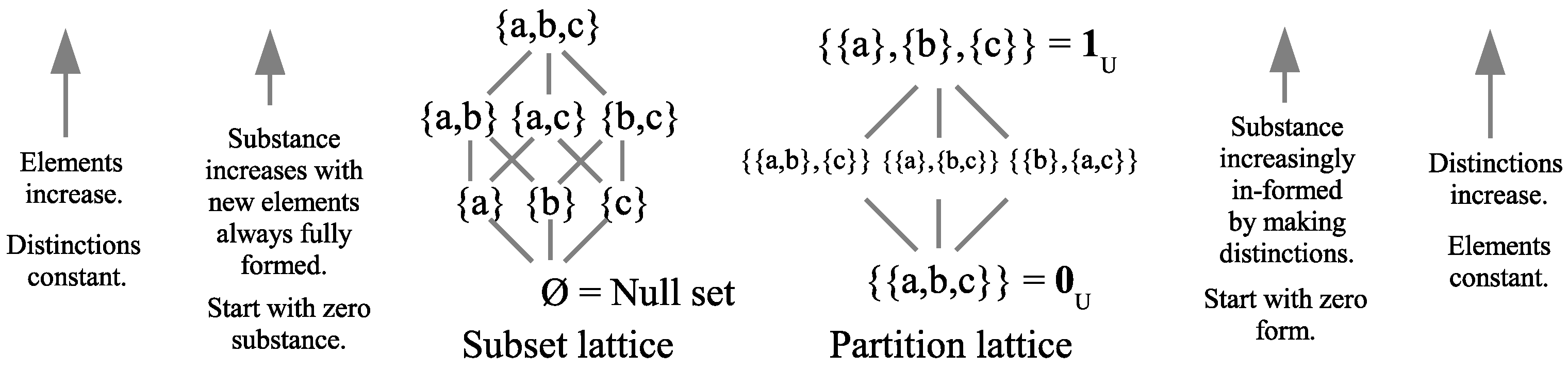
There is only one partition on a set that contains no superposition blocks (non-singleton blocks) and that is the discrete partition ${\mathbf{1}}_U$, where all the states are fully distinguished as singleton blocks. Leibniz used the Principle of Identity of Indistinguishables (PII) as a characterization of classical reality. Accordingly, the discrete partition (and only that partition) satisfies the partition logic version of the PII:

For any u,u′ ∈ U, if (u,u′) ∈ indit(1U), then u = u′

Principle of Identity of Indistinguishables in Partition Logic.

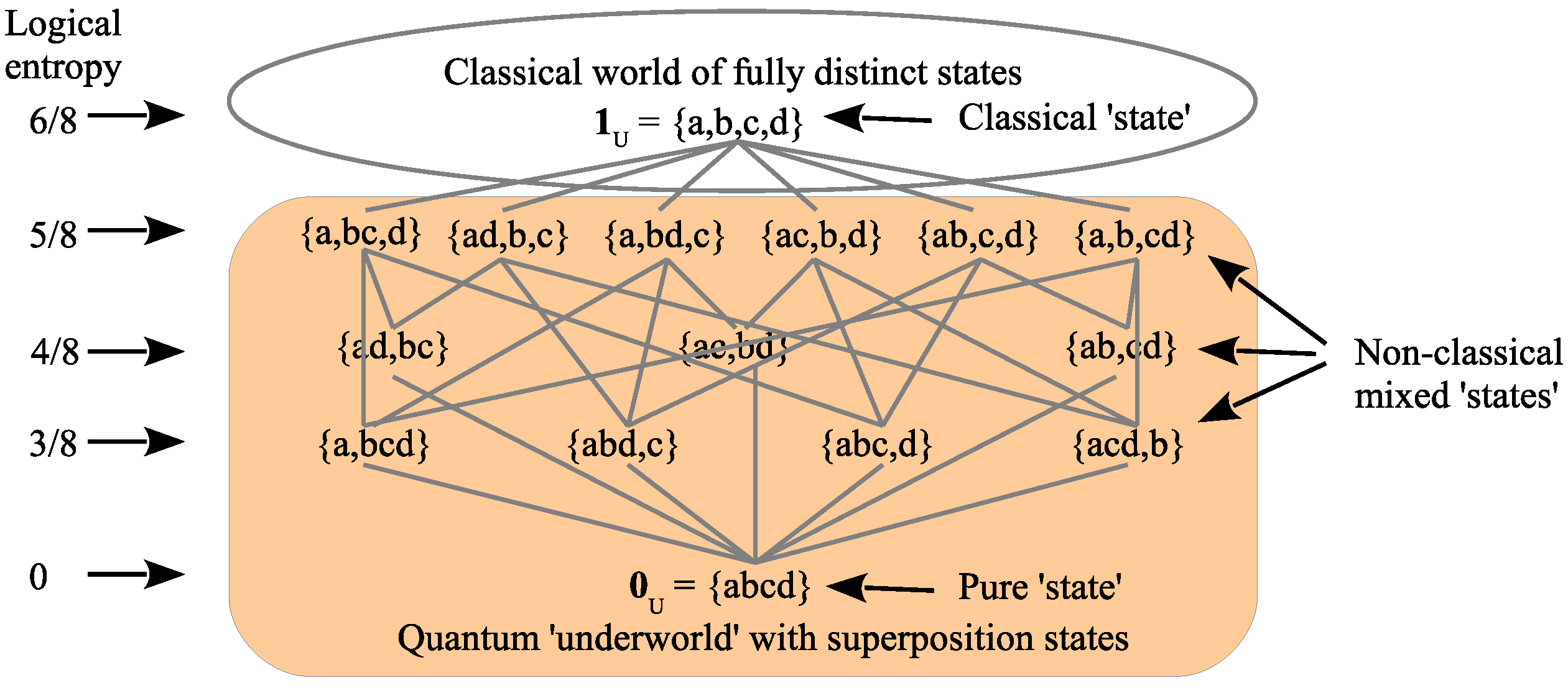
Thus, we can divide the partition lattice in the classical part (tip of the iceberg) and the quantum part (rest of the iceberg), where all the states include a superposition state, as illustrated in Figure 7 (with logical entropies based on an equiprobable assumption).

We begin building up the side-by-side dictionary by developing the set versions of the key QM concepts of quantum observables, quantum states, and quantum measurement.

3.4.2. Quantum Observables

We use a semi-algorithmic procedure to relate set concepts with the corresponding vector space concepts, where, for our purposes, the vector space is a Hilbert space. Such a procedure might be called a “yoga” [39] (p. 251). The key is to consider a set U first as just a set of elements at the set level and then as a basis set at the vector space level.

Yoga of Linearization:

Apply a set concept to U as a set,

and then the corresponding vector space concept

is whatever is linearly generated from the set concept

when U is taken as a basis set.

For instance, when a subset $S\subseteq U=\{u_1,\dots ,u_n\}$ taken as a subset of a basis set, then it generates a subspace $\left[S\right]$ of the Hilbert space $V=\left[U\right]$ and the cardinality $\left|S\right|$ of the subset correlates with the dimension $dim\left(\right[S\left]\right)$ of the subspace. Technically, the Yoga can be considered as an embellishment of the functor from the category of $Sets$ to the category of vector spaces over a given field, in our case the complex numbers $\mathbb{C}$. Given the vectors in a vector space represented in a certain basis U, the underlying set functor would take $\alpha |a\rangle +\beta |b\rangle$ to the support $\{a,b\}\subseteq U$.

If we start with a partition $\pi =\{B_1,\dots ,B_m\}$ on U, then applying that to a basis set of V, each block $B_j\in \pi$ generates a subspace $\left[B_j\right]$ and the collection of subspaces ${\left\{\left[B_j\right]\right\}}_{j=1}^m$ is a direct-sum decomposition or DSD of V, where DSD is defined as a set of subspaces so that each non-zero vector in the space can be uniquely represented as a sum of non-zero vectors from the subspaces in the set. Hence, a set partition correlates with a vector space DSD in our side-by-side dictionary. Indeed, we could have given a DSD-type definition of a set partition on U as a set of non-empty subsets ${\left\{B_j\right\}}_{j=1}^m$ such that every subset $S\subseteq U$ is uniquely represented as a union of non-empty subsets of the $B_j$’s. If the union of the $B_j$’s did not exhaust U, then $U-{\cup }_{j=1}^m{B}_j$ would have no representation, and if $B_j\cap B_k\ne \varnothing$, then that overlap would not have a unique representation. Hence, the DSD-type definition is equivalent to the usual definition as a set of non-empty subsets that exhaust U and are mutually disjoint.

In QM, the observables are Hermitian (or self-adjoint) operators $F:V\to V$, which have all eigenvalues as real numbers. The set correlate is a real-valued numerical attribute $f:U\to \mathbb{R}$. Given such a numerical attribute, the Yoga defines a Hermitian operator F by $F{u}_i=f\left(u_i\right)u_i$ on U as a basis set which then extends linearly to $F:V\to V$. The numerical attribute has an inverse-image partition $f^{-1}={\left\{f^{-1}\left(r\right)\right\}}_{r\in f\left(U\right)}$ and, by the Yoga, this generates the DSD ${\left\{V_r\right\}}_{r\in f\left(U\right)}$ of eigenspaces of F, where $V_r=\left[f^{-1}\left(r\right)\right]$. Given a Hermitian operator with an orthonormal (ON) basis U of eigenvectors, the numerical attribute f is recovered as the eigenvalue function $f:U\to \mathbb{R}$ that assigns each eigenvector in the basis to its eigenvalue. Thus, the set level correlate of an eigenvalue is a value of a real-valued numerical attribute.

What is the set level notion of an eigenvector? If we take “$rS$” to stand for “r is the value on the subset S”, then “$f\upharpoonright S=rS$” (where $f\upharpoonright S$ is f restricted to S) is the set version of the eigenvalue-eigenvector equation $F{u}_i=r{u}_i$. Then the set level eigenvectors are just the constant sets of f, the subsets on which f is constant (with some value r). The set level correlate of the eigenspace $V_r=\left[f^{-1}\left(r\right)\right]$ is the set of all constant subsets $\wp \left(f^{-1}\left(r\right)\right)$ (where we include ∅ as an honorary ‘eigenvector’).

Characteristic functions ${\chi }_S:U\to \{0,1\}\subseteq \mathbb{R}$, where ${\chi }_S\left(u_i\right)=1$ if $u_i\in S$, and 0 otherwise, define projection operators $P_{\left[S\right]}:V\to V$, which have only 0 or 1 eigenvalues. A Hermitian operator F, with eigenvalue function f, has a spectral decomposition as: $F={\sum }_{r\in f\left(U\right)}r{P}_{V_r}$, and the eigenvalue function or numerical attribute $f:U\to \mathbb{R}$ also has a ‘spectral decomposition’, where characteristic functions are substituted for the correlated projection operators, i.e., $f={\sum }_{r\in f\left(U\right)}r{\chi }_{f^{-1}\left(r\right)}:U\to \mathbb{R}$. Furthermore, given two sets U and $U^{\prime }$, we may form the set notion of the product $U\times U^{\prime }=\left\{(u,u^{\prime })\right|u\in U,u^{\prime }\in U^{\prime }\}$. Considering U and $U^{\prime }$ as a basis set for vector spaces V and $V^{\prime }$, we may apply the Yoga and the ordered pairs $(u,u^{\prime })$ (written as $u\otimes u^{\prime })$ bilinearly generate the tensor product $V\otimes V^{\prime }$.

We collect together these side-by-side correlates in partition math and QM math in

Table 3. Partition math for $f:U\to \mathbb{R}$ and corresponding QM math for $F:V\to V$.

Partition Math $\mathit{f}:\mathit{U}\to \mathbb{R}$	Hilbert Space Math $\mathit{F}:\mathit{V}\to \mathit{V}$
Partition ${\left\{f^{-1}\left(r\right)\right\}}_{r\in f\left(U\right)}$	DSD ${\left\{V_r\right\}}_{r\in f\left(U\right)}$
$U={\uplus }_{r\in f\left(U\right)}{f}^{-1}\left(r\right)$	$V={\oplus }_{r\in f\left(U\right)}{V}_r$
Numerical attribute $f:U\to \mathbb{R}$	Observable $F{u}_i=f\left(u_i\right)u_i$
$f\upharpoonright S=rS$	$F{u}_i=r{u}_i$
Constant set S of f	Eigenvector $u_i$ of F
Value r on constant set S	Eigenvalue r of eigenvector $u_i$
Characteristic fcn. ${\chi }_S:U\to \{0,1\}$	Projection operator $P_{\left[S\right]}{u}_i={\chi }_S\left(u_i\right)u_i$
Spectral Decomp. $f={\sum }_{r\in f\left(U\right)}r{\chi }_{f^{-1}\left(r\right)}$	Spectral Decomp. $F={\sum }_{r\in f\left(U\right)}r{P}_{V_r}$
Set of r-constant sets $\wp \left(f^{-1}\left(r\right)\right)$	Eigenspace $V_r=\left[f^{-1}\left(r\right)\right]$ of r -eigenvectors
Product $U\times U^{\prime }$	Tensor product $V\otimes V^{\prime }$

.

3.4.3. Quantum States

In ordinary mathematics. a real-valued random variable is a function $f:U\to \mathbb{R}$, where $U=\{u_1,...,u_n\}$ is an outcome set with point probabilities $p=(p_1,...,p_n)$. But it will be noted that probabilities played no role in the above treatment of quantum observables or their set correlates as real-valued numerical attributes. This is because in the comparison with real-valued random variables, quantum mechanics splits the two aspects between quantum observables (with no probabilities) and the quantum states which carry the probability information.

Hence, to build up the side-by-side correlates between partition math and QM math for quantum states, we begin with a universe set $U=\{u_1,...,u_n\}$ but with positive point probabilities $p=(p_1,...,p_n)$ (so U is an outcome space), and then we build the partition version of the quantum state. In QM math, there are two ways to represent a quantum state, as a state vector or as a density matrix. For our purposes, the density matrix [40] is far superior since the elements of the set level $n\times n$ density matrix can be one-to-one correlated with the distinctions and indistinctions of a partition in $U\times U$.

For a subset or event $S\subseteq U$, consider the $n\times 1$ column vector $|s\rangle$ whose $i^{th}$-entry is $\langle u_i|s\rangle =\sqrt{\frac{p_i}{Pr\left(S\right)}}$ if $u_i\in S$, and otherwise 0. Taking $\langle s|={|s\rangle }^t$ as the $1\times n$ row vector transpose of the normalized $|s\rangle$, we define the density matrix representation of the event S as the outer product:

$$\rho \left(S\right)=|s\rangle \langle s|.$$

Density matrices $\rho$ are called pure if ${\rho }^2=\rho$, and otherwise mixed. Since $|s\rangle$ is normalized, the inner product is $\langle s|s\rangle =1$ so $\rho {\left(S\right)}^2=|s\rangle \langle s|s\rangle \langle s|=|s\rangle \langle s|=\rho \left(S\right)$, so it is a pure state density matrix. The off-diagonal elements are $\rho {\left(S\right)}_{ik}=\frac{\sqrt{p_i{p}_k}}{Pr\left(S\right)}$ if $u_i,u_k\in S$ and 0 otherwise. This corresponds to the interpretation of S as a superposition subset since the non-zero off-diagonal elements indicate that the associated elements $u_i$ and $u_k$ are blurred, blobbed, or cohered together in a superposition. In QM math, the non-zero off-diagonal elements are called “coherences” indicating superposition, and, since superposition states are the characteristic non-classical states in QM, they account for the characteristic interference effects in QM.

For this reason, the off-diagonal terms of a density matrix… are often called “quantum coherences” because they are responsible for the interference effects typical of quantum mechanics that are absent in classical dynamics.

[41] (p. 177)

At the set level, $|s\rangle$ plays the role of the state vector or the so-called “wave function” even though there are no waves in sight in partition math.

It should be noted that the set version of the Born rule already appears since $Pr\left(u_i\right|S)={\langle u_i|s\rangle }^2$. It might be said that the Born rule was simply built into the definition of $|s\rangle$, but it still appears if we start with simply a pure state density matrix $\rho$. Since density matrices are positive and Hermitian, the eigenvalues of any density matrix are non-negative and sum to 1. The eigenvalues of a pure state density matrix $\rho$ are one 1 with the rest 0’s. If $|s\rangle$ is the normalized eigenvector associated with the eigenvalue 1, then it is the same as our previously defined $|s\rangle$ (up to sign), and the spectral decomposition of $\rho$ is $\rho =|s\rangle \langle s|$. Empirically, the Born rule does give the probability $Pr\left(u_i\right|S)$.

We now consider a partition $\pi =\{B_1,...,B_m\}$ on U and define the pure state density matrices $\rho \left(B_j\right)=|b_j\rangle \langle b_j|$ by taking $S=B_j$ with $|s\rangle$ then denoted $|b_j\rangle$. Then, the set level density matrix for $\pi$ is the probabilistic sum of the $\rho \left(B_j\right)$ matrices:

$$\rho \left(\pi \right)={\sum }_{j=1}^{m}Pr\left(B_j\right)\rho \left(B_j\right),$$

which is a mixed state density matrix except in the case $\pi ={\mathbf{0}}_U$ which is pure. All the properties of the partition $\pi$ are now expressed in a density matrix form at the set level. For instance, the entries in $\rho \left(\pi \right)$ are $\rho {\left(\pi \right)}_{ik}=\sqrt{p_i{p}_k}$ if $(u_i,u_k)\in indit\left(\pi \right)$ and 0 otherwise. Thus, the non-zero entries represent the indistinctions of $\pi$ and the zero entries represents the distinctions. The point probabilities are along the diagonal of $\rho \left(\pi \right)$ and the n eigenvalues of $\rho \left(\pi \right)$ are the m block probabilities $Pr\left(B_j\right)$ and $n-m$ 0’s and the associated ON eigenvectors are the m$|b_j\rangle$ vectors and $n-m$ other ON vectors; so, the spectral decomposition is: $\rho \left(\pi \right)={\sum }_{j=1}^{m}Pr\left(B_j\right)|b_j\rangle \langle b_j|$. Since the blocks of $\pi$ are disjoint, the normalized vectors $|b_j\rangle$ are mutually orthogonal, so $\langle b_k|b_j\rangle ={\delta }_{ki}$.

Now that we have converted the set level machinery of partition math into a density matrix format, the rest of the argument that QM math is just the Hilbert space version of the partition math is trivial. In a (n-dimensional) Hilbert space, an arbitrary density matrix $\rho$ has an orthonormal basis of eigenvectors $\left\{\right|u_i\rangle {\}}_{i=1}^n$ with n non-negative eigenvalues ${\lambda }_1,...,{\lambda }_n$, which sum to 1 and the spectral decomposition is: $\rho ={\sum }_{i=1}^n{\lambda }_i|u_i\rangle \langle u_i|$. These and the correlations for pure state density matrices $\rho \left(\psi \right)$ are given in

Table 4. Quantum states: partition math and QM math.

Partition Math	Hilbert Space Math
Density matrix: $\rho \left(\pi \right)$	$\rho$
ON eigenvectors: $\langle b_k|b_j\rangle ={\delta }_{kj}$	$\langle u_k|u_i\rangle ={\delta }_{ki}$
Eigenvalues: $Pr\left(B_1\right),...,Pr\left(B_m\right),0,...,0$	${\lambda }_1,...,{\lambda }_n$
Spectral decomp.: $\rho \left(\pi \right)={\sum }_{j=1}^{m}Pr\left(B_j\right)|b_j\rangle \langle b_j|$	$\rho ={\sum }_{i=1}^n{\lambda }_i|u_i\rangle \langle u_i|$
Non-zero off-diagonal entry: Cohering of diag. states	Cohering of diagonal states
Pure state: $\rho \left(S\right)=|s\rangle \langle s|$	$\rho \left(\psi \right)=|\psi \rangle \langle \psi |$
Eigenvector Eigenvalue 1 State vector: $|s\rangle$	$|\psi \rangle$
Born Rule: $Pr\left(u_i\right|S)={\langle u_i|s\rangle }^2$	$Pr\left(u_i\right|\psi )={\left|\langle u_i|\psi \rangle \right|}^2$

.

3.4.4. Quantum Measurement

A quantum measurement (always projective) can be described at the quantum level by the Lüders mixture operation ([42,43]). Given an observable $F:V\to V$ with projections ${\left\{P_{V_r}\right\}}_{r\in f\left(U\right)}$ to the eigenspaces ${\left\{V_r\right\}}_{r\in f\left(U\right)}$ with an ON basis of eigenvectors U, the result of measuring a quantum state given by a density matrix $\rho$, expressed in the measurement basis U, is the post-measurement density matrix $\widehat{\rho }$ given by:

$$\widehat{\rho }={\sum }_{r\in f\left(U\right)}{P}_{V_r}\rho P_{V_r}.$$

Hilbert space Lüders mixture operation

The Lüders mixture operation creates a mixed state, a set of states, one of which occurs with the probabilities given by the Born rule. That process is overall described as the infamous ‘quantum jump’.

We have already built up the side-by-side correlation tables between partition math and QM math, so we know how to formulate the set level version of the Lüders mixture operation. Given a numerical attribute $f:U\to \mathbb{R}$ with the inverse-image partition $f^{-1}={\left\{f^{-1}\left(r\right)\right\}}_{r\in f\left(U\right)}$ playing the role of the observable and the state $\rho \left(\pi \right)$ playing the role of the state being measured, we can compute the effect of the set level measurement. Let $P_{f^{-1}\left(r\right)}$ be the $n\times n$ projection matrix, which is a diagonal matrix with the diagonal entries being ${\chi }_{f^{-1}\left(r\right)}\left(u_i\right)$. Then, the Lüders mixture operation at the set level is:

$$\widehat{\rho }\left(\pi \right)={\sum }_{r\in f\left(U\right)}{P}_{f^{-1}\left(r\right)}\rho \left(\pi \right)P_{f^{-1}\left(r\right)}.$$

What is the result of measuring the partition-based state $\rho \left(\pi \right)$ by the numerical attribute f which defines the partition $f^{-1}={\left\{f^{-1}\left(r\right)\right\}}_{r\in f\left(U\right)}$? It is easily shown that:

$$\widehat{\rho }\left(\pi \right)=\rho (\pi \vee f^{-1})$$

Set level Lüders mixture operation.

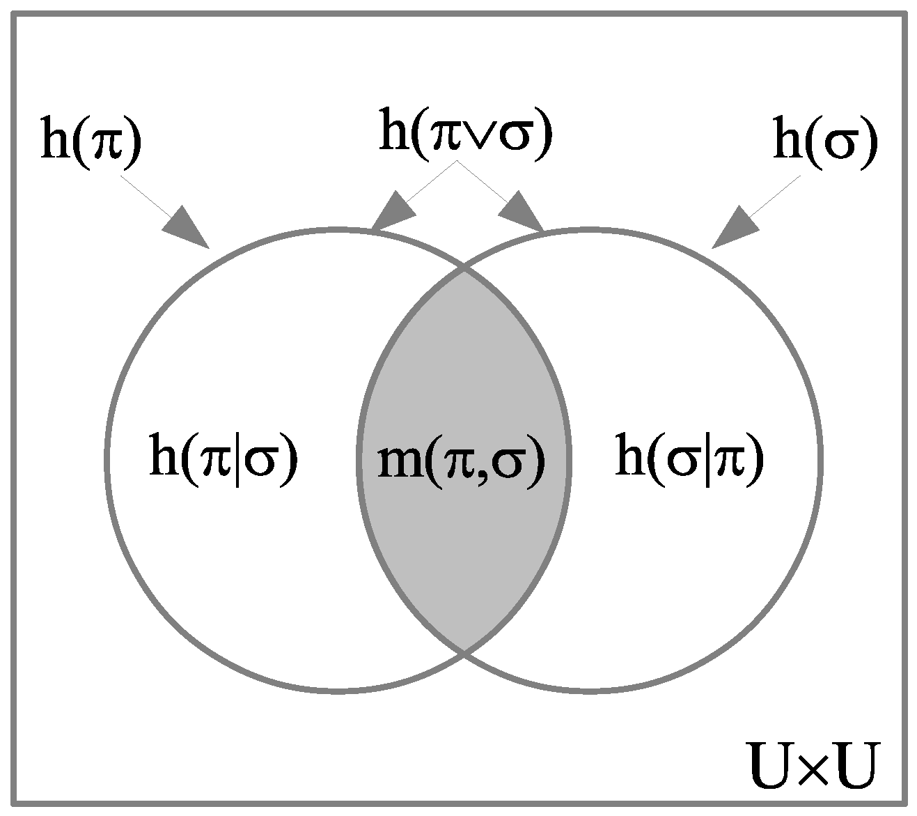
Thus, the effect of (projective) measurement at the set level is to go from a state given by $\pi$ to the more refined state $\pi \vee f^{-1}$. The increase in logical entropy is: $h(\pi \vee f^{-1})-h\left(\pi \right)=h\left(f^{-1}\right|\pi )$ (as one can see from the Venn diagram of Figure 2 with $\sigma =f^{-1}$. Moreover, that difference can be read off of the difference between the pre-measurement $\rho \left(\pi \right)$ and the post-measurement $\widehat{\rho }\left(\pi \right)=\rho (\pi \vee f^{-1})$. Logical entropy is the value of product measure $p\times p$ on the ditsets and the ditsets are given by the zeros in the density matrices. Hence, we consider all the indits given by non-zero entries $\sqrt{p_i{p}_k}$ in $\rho \left(\pi \right)$ that were turned into dits (i.e., zeroed) in $\rho (\pi \vee f^{-1})$. The squares $p_i{p}_k$ of all those zeroed entries is the value of the product measure $p\times p$ on the additional dits created in the measurement, which is just $h\left(f^{-1}\right|\pi )=p\times p[dit\left(f^{-1}\right)-dit\left(\pi \right)]$. The analogous theorem holds for quantum logical entropy for the projective measurement process in QM math ([1,28]).

This completes the argument that the QM math of quantum states, quantum observables, and quantum measurement is just the Hilbert space version of the math of partitions. The results are given in the side-by-side dictionary of

Table 5. Three basic notions: partition version and QM math version.

Dictionary	Partition Math	Hilbert Space Math
Notion of state	$\rho \left(\pi \right)={\sum }_{j=1}^{m}Pr\left(B_j\right)|b_j\rangle \langle b_j|$	$\rho ={\sum }_{i=1}^n{\lambda }_i|u_i\rangle \langle u_i|$
Notion of observable	$f={\sum }_{r\in f\left(U\right)}r{\chi }_{f^{-1}\left(r\right)}:U\to \mathbb{R}$	$F={\sum }_{r\in f\left(U\right)}r{P}_{V_r}$
Notion of measurement	$\widehat{\rho }\left(\pi \right)={\sum }_{r\in f\left(U\right)}{P}_{f^{-1}\left(r\right)}\rho \left(\pi \right)P_{f^{-1}\left(r\right)}$	$\widehat{\rho }={\sum }_{r\in f\left(U\right)}{P}_{V_r}\rho P_{V_r}$

.

A numerical example. These results can be illustrated with a simple example. Let $U=\{a,b,c\}$ with the point probabilities $p_a=\frac{1}{2}$, $p_b=\frac{1}{3}$, and $p_c=\frac{1}{6}$. We first construct the density matrix $\rho \left(\pi \right)$ for the partition $\pi =\{B_1,B_2\}=\{\{a,c\},\left\{b\right\}\}$. Then, we have:

$$|b_1\rangle =\left[\begin{array}{c}\sqrt{\frac{1/2}{2/3}}\\ 0\\ \sqrt{\frac{1/6}{2/3}}\end{array}\right]=\left[\begin{array}{c}\frac{\sqrt{3}}{2}\\ 0\\ \frac{1}{2}\end{array}\right] \mathrm{and} |b_2\rangle =\left[\begin{array}{c}0\\ \sqrt{\frac{1/3}{1/3}}\\ 0\end{array}\right]=\left[\begin{array}{c}0\\ 1\\ 0\end{array}\right]$$

so that the two pure state density matrices are:

$$|b_1\rangle \langle b_1|=\left[\begin{array}{c}\frac{\sqrt{3}}{2}\\ 0\\ \frac{1}{2}\end{array}\right]\left[\begin{array}{ccc}\frac{\sqrt{3}}{2}& 0& \frac{1}{2}\end{array}\right]=\left[\begin{array}{ccc}\frac{3}{4}& 0& \frac{\sqrt{3}}{4}\\ 0& 0& 0\\ \frac{\sqrt{3}}{4}& 0& \frac{1}{4}\end{array}\right] \mathrm{and} |b_2\rangle \langle b_2|=\left[\begin{array}{ccc}0& 0& 0\\ 0& 1& 0\\ 0& 0& 0\end{array}\right].$$

Then, $\rho \left(\pi \right)$ is the probabilistic sum:

$$\rho \left(\pi \right)={\sum }_{j=1}^2\rho \left(B_j\right){\displaystyle |}{b}_j\rangle \langle b_j{\displaystyle |}=\frac{2}{3}\left[\begin{array}{ccc}\frac{3}{4}& 0& \frac{\sqrt{3}}{4}\\ 0& 0& 0\\ \frac{\sqrt{3}}{4}& 0& \frac{1}{4}\end{array}\right]+\frac{1}{3}\left[\begin{array}{ccc}0& 0& 0\\ 0& 1& 0\\ 0& 0& 0\end{array}\right]=\left[\begin{array}{ccc}\frac{1}{2}& 0& \frac{1}{2\sqrt{3}}\\ 0& \frac{1}{3}& 0\\ \frac{1}{2\sqrt{3}}& 0& \frac{1}{6}.\end{array}\right]$$

With $\pi =\left\{\right\{a,c\},\{b\left\}\right\}$, we have: $indit\left(\pi \right)=\left\{\right(a,a),(b,b),(c,c),(a,c),(c,a\left)\right\}$, which corresponds to the five non-zero entries in $\rho \left(\pi \right)$—and thus the zero entries correspond to the ditset: $dit\left(\pi \right)=\left\{\right(a,b),(b,a),(b,c),(c,b\left)\right\}$.

The orthogonal eigenvectors of $\rho \left(\pi \right)$ are:

$$\left\{\left[\begin{array}{c}-\frac{1}{\sqrt{3}}\\ 0\\ 1\end{array}\right]\right\}\leftrightarrow 0,\left\{\left[\begin{array}{c}\sqrt{3}\\ 0\\ 1\end{array}\right]\right\}\leftrightarrow \frac{2}{3},\left\{\left[\begin{array}{c}0\\ 1\\ 0\end{array}\right]\right\}\leftrightarrow \frac{1}{3},$$

the non-zero eigenvalues are the block probabilities $Pr\left(B_1\right)$ and $Pr\left(B_2\right)$, and the eigenvectors for those non-zero eigenvalues normalize to $|b_1\rangle$ and $|b_2\rangle$.

Let $f:U\to \mathbb{R}$ be the numerical attribute where $f\left(a\right)=f\left(b\right)=1$ and $f\left(c\right)=0$; so, the inverse-image partition is $f^{-1}=\{\{a,b\},\left\{c\right\}\}$. The projection matrices for the blocks are:

$$P_{\{a,b\}}=\left[\begin{array}{ccc}1& 0& 0\\ 0& 1& 0\\ 0& 0& 0\end{array}\right] \mathrm{and} P_{\left\{c\right\}}=\left[\begin{array}{ccc}0& 0& 0\\ 0& 0& 0\\ 0& 0& 1\end{array}\right]$$

so, the set version of the Lüders mixture operation is:

$$P_{\{a,b\}}\rho \left(\pi \right)P_{\{a,b\}}+P_{\left\{c\right\}}\rho \left(\pi \right)P_{\left\{c\right\}}$$

$$=\left[\begin{array}{ccc}1& 0& 0\\ 0& 1& 0\\ 0& 0& 0\end{array}\right]\left[\begin{array}{ccc}\frac{1}{2}& 0& \frac{1}{2\sqrt{3}}\\ 0& \frac{1}{3}& 0\\ \frac{1}{2\sqrt{3}}& 0& \frac{1}{6}\end{array}\right]\left[\begin{array}{ccc}1& 0& 0\\ 0& 1& 0\\ 0& 0& 0\end{array}\right]+\left[\begin{array}{ccc}0& 0& 0\\ 0& 0& 0\\ 0& 0& 1\end{array}\right]\left[\begin{array}{ccc}\frac{1}{2}& 0& \frac{1}{2\sqrt{3}}\\ 0& \frac{1}{3}& 0\\ \frac{1}{2\sqrt{3}}& 0& \frac{1}{6}\end{array}\right]\left[\begin{array}{ccc}0& 0& 0\\ 0& 0& 0\\ 0& 0& 1\end{array}\right]$$

$$=\left[\begin{array}{ccc}\frac{1}{2}& 0& 0\\ 0& \frac{1}{3}& 0\\ 0& 0& 0\end{array}\right]+\left[\begin{array}{ccc}0& 0& 0\\ 0& 0& 0\\ 0& 0& \frac{1}{6}\end{array}\right]=\left[\begin{array}{ccc}\frac{1}{2}& 0& 0\\ 0& \frac{1}{3}& 0\\ 0& 0& \frac{1}{6}\end{array}\right]=\widehat{\rho }\left(\pi \right).$$

The first thing to check is $\widehat{\rho }\left(\pi \right)=\rho (\pi \vee f^{-1})$? The join is:

$$\pi \vee f^{-1}=\{\{a,c\},\left\{b\right\}\}\vee \{\{a,b\},\left\{c\right\}\}=\{\left\{a\right\},\left\{b\right\},\left\{c\right\}\}={\mathbf{1}}_U$$

as illustrated in Figure 8.

Then, it is clear that $\widehat{\rho }\left(\pi \right)=\rho (\pi \vee f^{-1})=\rho \left({\mathbf{1}}_U\right)$ since there are no non-zero off-diagonal elements indicating no superpositions in the partition, i.e., the discrete partition ${\mathbf{1}}_U$. Furthermore, we can check that the increase in logical entropy from $\rho \left(\pi \right)$ to $\widehat{\rho }\left(\pi \right)$ is equal to the sum of the squares of the ‘coherence’ entries that were ‘decohered’, i.e., zeroed in the measurement. The logical entropy of $\pi$ is:

$$h\left(\pi \right)=1-{\left(\frac{2}{3}\right)}^2-{\left(\frac{1}{3}\right)}^2=1-\frac{4}{9}-\frac{1}{9}=\frac{4}{9}.$$

The logical entropy of ${\mathbf{1}}_U$ is:

$$h\left({\mathbf{1}}_U\right)=1-{\left(\frac{1}{2}\right)}^2-{\left(\frac{1}{3}\right)}^2-{\left(\frac{1}{6}\right)}^2=1-\frac{1}{4}-\frac{1}{9}-\frac{1}{36}=1-\frac{14}{36}=\frac{11}{18}$$

so, the increase in logical entropy due to the measurement is:

$$h\left({\mathbf{1}}_U\right)-h\left(\pi \right)=\frac{11}{18}-\frac{8}{18}=\frac{3}{18}=\frac{1}{6}.$$

In the transition from $\rho \left(\pi \right)$ to $\widehat{\rho }\left(\pi \right)$, there were two non-zero coherence terms with the value of $\frac{1}{2\sqrt{3}}$ which were zeroed (i.e., those indits were decohered into dits), so the sum of their squares is: ${\left(\frac{1}{2\sqrt{3}}\right)}^2+{\left(\frac{1}{2\sqrt{3}}\right)}^2=\frac{1}{12}+\frac{1}{12}=\frac{1}{6}$. ✓

3.4.5. ‘Quantum Mechanics’ Over Sets

Now that we have established a basic dictionary to translate between partition math and QM math, we can start to use the partition math to help explain in relatively simple and intuitive terms, some of the more vexing aspects of QM. But there is one aspect of QM math that we have not yet given a set-based version for, and that is the existence of different bases since the QM math is formulated in a vector space.

The solution is that the set-based math can also be formulated in the vector space, where the vectors stand for subsets, name vector spaces over ${\mathbb{Z}}_2=\{0,1\}$. Addition modulo two is like normal addition except that $1+1=0$. To represent the subsets of U in vector space terms, we may work in ${\mathbb{Z}}_2^n$, where the vectors are $n\times 1$ column vectors with $0,1$ entries and modulo two addition of components. The canonical basis vectors are the column vectors $|u_i\rangle$ with a 1 in the $i^{th}$ place and otherwise 0’s; so, a subset $S\subseteq U$ would be represented on this basis by the column vector $|S\rangle$ with the $i^{th}$ entry ${\chi }_S\left(u_i\right)$. Given the vector $|T\rangle$ for $T\subseteq U$, the sum $|S\rangle +|T\rangle$ would have cancellation on the overlap $S\cap T$; so, the sum is the vector for the symmetric difference $S\Delta T=(S\cup T)-(S\cap T)=(S-T)\cup (T-S)$ so, $|S\rangle +|T\rangle =|S\Delta T\rangle$. By associating the canonical basis vectors $|u_i\rangle$ with the singletons $\left\{u_i\right\}\in \wp \left(U\right)$, we can transfer the vector space structure on ${\mathbb{Z}}_2^n$ to $\wp \left(U\right)$, where the subset addition operation in $\wp \left(U\right)$ as a vector space is $S+T=S\Delta T$; so, we have an isomorphism of vector spaces ${\mathbb{Z}}_2^n\cong \wp \left(U\right)$. In this manner, we can build up a toy or pedagogical model of QM called “Quantum Mechanics over Sets” or QM/Sets ([1,44]).

To keep matters simple, let us take $U=\{a,b,c\}$ and then the singletons $\left\{a\right\}$, $\left\{b\right\}$, and $\left\{c\right\}$ are a basis set for the $2^3=8$ vectors in the 3-dimensional vector space $\wp \left(U\right)$—a basis that we can treat as the computational basis. Now, there are other basis sets, such as $U^{\prime }=\{a^{\prime },b^{\prime },c^{\prime }\}$, where $\left\{a^{\prime }\right\}=\{a,b\}$, $\left\{b^{\prime }\right\}=\{a,b,c\}$, and $\left\{c^{\prime }\right\}=\{b,c\}$. The $U^{\prime }$ vectors form a basis since:

$\{a^{\prime },b^{\prime }\}=\{a,b\}+\{a,b,c\}=\left\{c\right\}$,

$\{b^{\prime },c^{\prime }\}=\{a,b,c\}+\{b,c\}=\left\{a\right\}$, and $\{a^{\prime },b^{\prime },c^{\prime }\}=\{a,b\}+\{a,b,c\}+\{b,c\}=\left\{b\right\}$.

Table 6. Ket table giving a vector space isomorphism: ${\mathbb{Z}}_2^3\cong \wp \left(U\right)\cong \wp \left(U^{\prime }\right)\cong \wp \left(U^{″}\right)$ where row = ket.

${\mathbb{Z}}_2^3$	$\mathit{U}=\{\mathit{a},\mathit{b},\mathit{c}\}$	${\mathit{U}}^{\prime }=\{{\mathit{a}}^{\prime },{\mathit{b}}^{\prime },{\mathit{c}}^{\prime }\}$	${\mathit{U}}^{″}=\{{\mathit{a}}^{″},{\mathit{b}}^{ȃ},{\mathit{c}}^{″}\}$
${[1,1,1]}^t$	$\{a,b,c\}$	$\left\{b^{\prime }\right\}$	$\{a^{″},b^{″},c^{″}\}$
${[1,1,0]}^t$	$\{a,b\}$	$\left\{a^{\prime }\right\}$	$\left\{b^{″}\right\}$
${[0,1,1]}^t$	$\{b,c\}$	$\left\{c^{\prime }\right\}$	$\{b^{″},c^{″}\}$
${[1,0,1]}^t$	$\{a,c\}$	$\{a^{\prime },c^{\prime }\}$	$\left\{c^{″}\right\}$
${[1,0,0]}^t$	$\left\{a\right\}$	$\{b^{\prime },c^{\prime }\}$	$\left\{a^{″}\right\}$
${[0,1,0]}^t$	$\left\{b\right\}$	$\{a^{\prime },b^{\prime },c^{\prime }\}$	$\{a^{″},b^{″}\}$
${[0,0,1]}^t$	$\left\{c\right\}$	$\{a^{\prime },b^{\prime }\}$	$\{a^{″},c^{″}\}$
${[0,0,0]}^t$	∅	∅	∅

lists the eight vectors expressed in three different bases, where each row represents the same abstract vector or “ ket”, so it is a ket table.

3.4.6. A Pedagogical Model of the Two-Slit Experiment

One simple application of this set level framework is to build a pedagogical model of the two-slit experiment, an experiment that Richard Feynman said “ has in it the heart of quantum mechanics” and the “only mystery” [45] (Section 1-1). We have already seen how quantum measurement looks at the set level. The transition of an isolated system in QM without any measurements (state reductions) is described as a unitary transformation, which is a linear transformation that preserves inner products and thus maps an ON basis to an ON basis. There are no inner products in vector spaces over finite fields, so the corresponding type of transformation would just be a non-singular one that transforms a basis into a basis, e.g., transforms the U-basis into the $U^{\prime }$-basis. Indeed, in our model of the two-slit experiment, we will assume that ‘dynamics’ for each time period, i.e., $\left\{a\right\}⇝\left\{a^{\prime }\right\}=\{a,b\}$, $\left\{b\right\}⇝\left\{b^{\prime }\right\}=\{a,b,c\}$, and $\left\{c\right\}⇝\left\{c^{\prime }\right\}=\{b,c\}$. 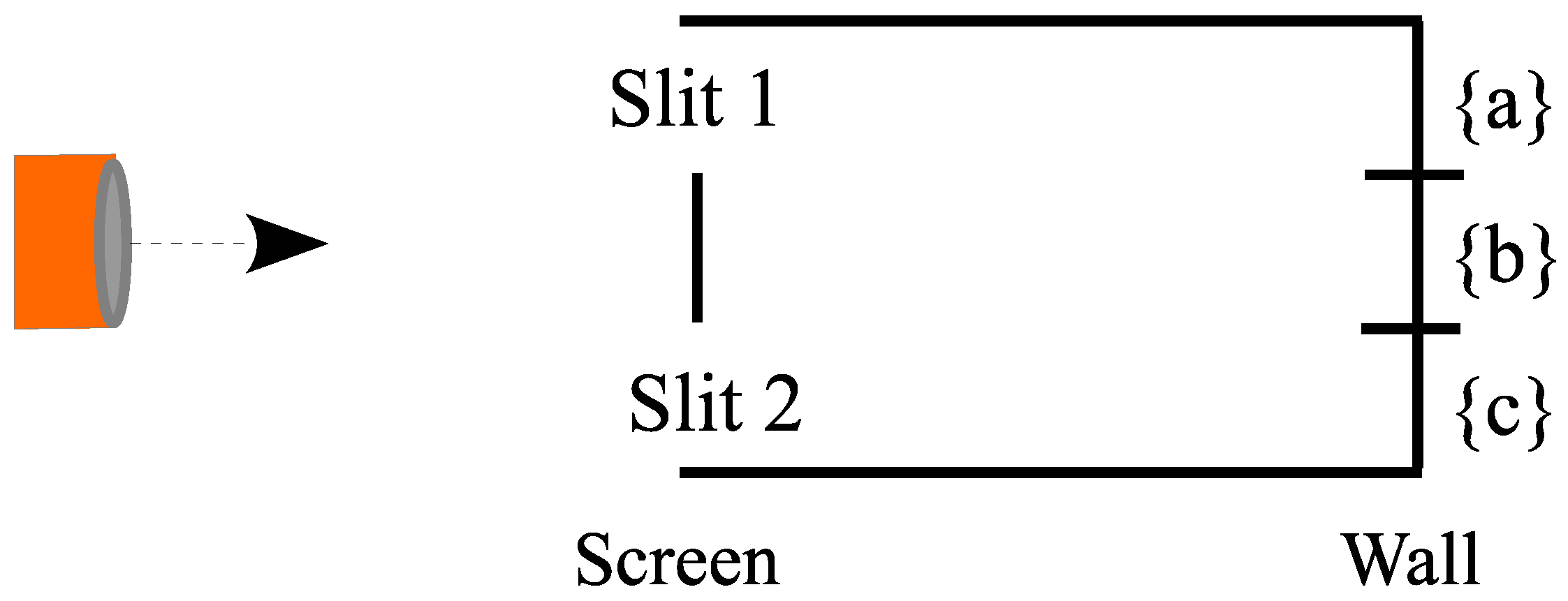There are three (equiprobable) states of $U=\{a,b,c\}$ that a particle can have which are the vertical positions as pictured in Figure 9 for the initial setup for the experiment. We could think of the vertical positions as having numerical values 3, 2, and 1, respectively, but the letters will suffice for a pedagogical model.

The two slits are in the screen at positions $\left\{a\right\}$ and $\left\{c\right\}$, and the detection wall can record a particle hitting at positions $\left\{a\right\}$, $\left\{b\right\}$, or $\left\{c\right\}$. A particle emerges at the source on the left at $\left\{b\right\}$ and in one time period evolves to the state $\left\{b^{\prime }\right\}=\{a,b,c\}$. The particle in that superposition state $\{a,b,c\}$ has its first state reduction at the screen. If it hits the screen at $\left\{b\right\}$, then it does not proceed on to the detection wall. Otherwise, the particle is reduced to the superposition state $\{a,c\}$ at the screen, i.e., a superposition of Slit 1 and Slit 2.

Starting with the superposition $\{a,c\}$ at the screen, we need to consider two cases: Case 1 where there are detectors at the slits so there is a state reduction to $\left\{a\right\}$ or $\left\{c\right\}$ with equal $\frac{1}{2}$ probability, or Case 2 where there is no detection at the screen.

Case 1: Starting with $\{a,c\}$ at the screen, with detectors, there is a half-half probability of the particle being detected at each of the slits and then it evolves according to the dynamics to the detection wall. If it went through Slit 1 at $\left\{a\right\}$, then it evolves to $\left\{a^{\prime }\right\}=\{a,b\}$ and hits the detection wall with equal probability at $\left\{a\right\}$ or $\left\{b\right\}$. If it went through Slit 2 at $\left\{c\right\}$, then it evolves to $\left\{c^{\prime }\right\}=\{b,c\}$ and hits the detection wall with equal probability at $\left\{b\right\}$ or $\left\{c\right\}$. Then, we add up the final probabilities at the detection wall as follows:

$Pr\left(\right\{a\left\}\mathrm{at}\mathrm{wall}\right|\{a,c\}\mathrm{at}\mathrm{screen})$

$=Pr\left(\right\{a\left\}\mathrm{at}\mathrm{screen}\right|\{a,c\}\mathrm{at}\mathrm{screen})Pr(\left\{a\right\}\mathrm{at}\mathrm{wall}\left|\right\{a\left\}\mathrm{at}\mathrm{screen}\right)$

$=\frac{1}{2}\times \frac{1}{2}=\frac{1}{4}$;

$Pr\left(\right\{b\left\}\mathrm{at}\mathrm{wall}\right|\{a,c\}\mathrm{at}\mathrm{screen})$

$=Pr\left(\right\{a\left\}\mathrm{at}\mathrm{screen}\right|\{a,c\}\mathrm{at}\mathrm{screen})Pr(\left\{b\right\}\mathrm{at}\mathrm{wall}\left|\right\{a\left\}\mathrm{at}\mathrm{screen}\right)$

$+Pr\left(\right\{c\left\}\mathrm{at}\mathrm{screen}\right|\{a,c\}\mathrm{at}\mathrm{screen})Pr(\left\{b\right\}\mathrm{at}\mathrm{wall}\left|\right\{c\left\}\mathrm{at}\mathrm{screen}\right)$

$=\frac{1}{2}\times \frac{1}{2}+\frac{1}{2}\times \frac{1}{2}=\frac{1}{2}$; and

$Pr\left(\right\{c\left\}\mathrm{at}\mathrm{wall}\right|\{a,c\}\mathrm{at}\mathrm{screen})$

$=Pr\left(\right\{c\left\}\mathrm{at}\mathrm{screen}\right|\{a,c\}\mathrm{at}\mathrm{screen})Pr(\left\{c\right\}\mathrm{at}\mathrm{wall}\left|\right\{c\left\}\mathrm{at}\mathrm{screen}\right)$

$=\frac{1}{2}\times \frac{1}{2}=\frac{1}{4}$.

Hence, Case 1 of detectors at the screen, gives the probability distribution pictured in Figure 10.

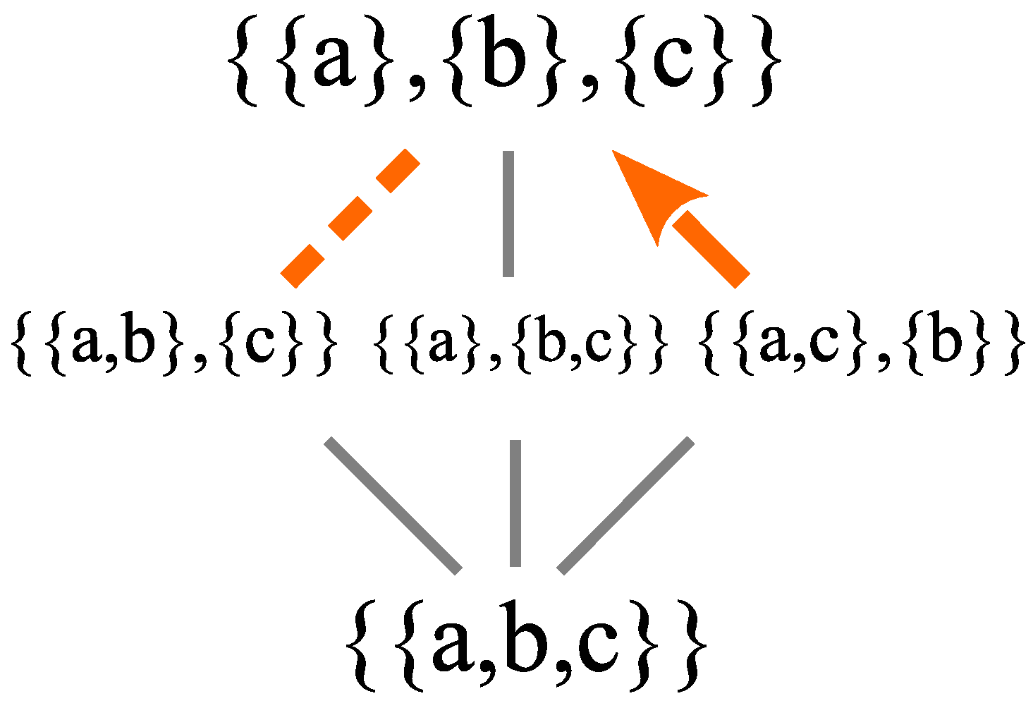
The partition lattice for $U=\{a,b,c\}$ provides an anschaulich or intuitive picture of these processes where $\{a,c\}$ at the screen reduces (i.e., “quantum jumps”) to the classical states $\left\{a\right\}$ or $\left\{c\right\}$, i.e., the particle goes through Slit 1 or through Slit 2, and evolves to either $\left\{a^{\prime }\right\}$ or $\left\{c^{\prime }\right\}$, as illustrated in Figure 11.

Case 2: Starting with the superposition $\{a,c\}$ at the screen, if there are not detectors at the slits, then the superposition evolves linearly according to the dynamics:

$$\{a,c\}=\left\{a\right\}+\left\{c\right\}⇝\left\{a^{\prime }\right\}+\left\{c^{\prime }\right\}=\{a,b\}+\{b,c\}=\{a,c\}.$$

Then, the probabilities at the detection wall are:

$Pr\left(\right\{a\left\}\mathrm{at}\mathrm{wall}\right|\{a,c\}\mathrm{at}\mathrm{screen})$

$=Pr\left(\right\{a\left\}\mathrm{at}\mathrm{wall}\right|\{a,c\}\mathrm{at}\mathrm{wall})Pr(\{a,c\}\mathrm{at}\mathrm{wall}\left|\right\{a,c\left\}\mathrm{at}\mathrm{screen}\right)$

$=\frac{1}{2}\times 1=\frac{1}{2}$;

$Pr\left(\right\{b\left\}\mathrm{at}\mathrm{wall}\right|\{a,c\}\mathrm{at}\mathrm{screen})$

$=Pr\left(\right\{b\left\}\mathrm{at}\mathrm{wall}\right|\{a,c\}\mathrm{at}\mathrm{wall})Pr(\{a,c\}\mathrm{at}\mathrm{wall}\left|\right\{a,c\left\}\mathrm{at}\mathrm{screen}\right)$

$=0\times 1=0$; and

$Pr\left(\right\{c\left\}\mathrm{at}\mathrm{wall}\right|\{a,c\}\mathrm{at}\mathrm{screen})$

$=Pr\left(\right\{c\left\}\mathrm{at}\mathrm{wall}\right|\{a,c\}\mathrm{at}\mathrm{wall})Pr(\{a,c\}\mathrm{at}\mathrm{wall}\left|\right\{a,c\left\}\mathrm{at}\mathrm{screen}\right)$

$=\frac{1}{2}\times 1=\frac{1}{2}$.

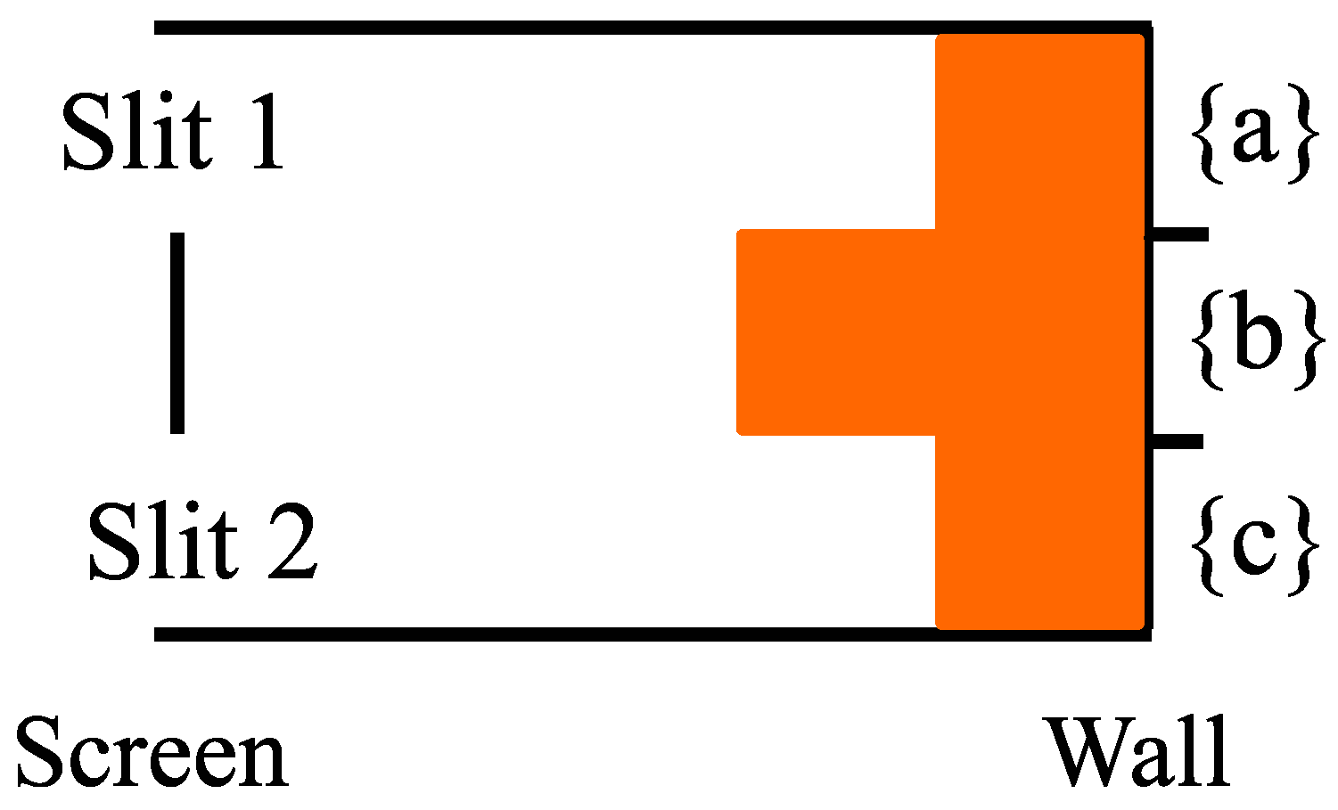
Hence, Case 2 of no detectors at the screen, gives the probability distribution pictured in Figure 12.

Figure 10 shows the probability stripes characteristic of the full QM two-slit experiments with no detectors at the slits. The stripes are due to the interference in the evolving superposition state, i.e., $\{a,c\}⇝\{a^{\prime },c^{\prime }\}=\{a,b\}+\{b,c\}=\{a,c\}$, where the $\left\{b\right\}$’s destructively interfere in the modulo two addition of the model. Since there were no state reductions (or ‘measurements’) at the screen, the evolution was from the superposition state $\{a,c\}$ to the superposition state $\{a^{\prime },c^{\prime }\}$, all at the non-classical quantum level, as illustrated in Figure 13–not at the classical level that is crossed out.

One of the important ‘takeaways’ of the partition analysis is that there are different levels of reality (Figure 7), and yet our intuitions only see reality in classical terms as fully definite. Thus, in case two, there is no state reduction at the screen (since there are no detectors), so the evolution of the superposition takes place at a non-classical level (Figure 13) without ever achieving the definiteness of “going through Slit 1” or “going through Slit” as in Case 1.

The great sticking point in the “mystery” of the two-slit experiment is that question: “Which slit did the particle do through to get to the detection wall in the case of no detectors?” This is the question that has gone unanswered for a century. The implicit classical assumption is that evolution has to be at the fully definite (“It has to go through one slit or the other”) classical level. Feynman stated that intuitive assumption as: “Proposition A: Either an electron goes through hole No. 1 or it goes through hole No. 2”. And then he showed that “Proposition A is false” [46] (pp. 139–140). If the particle did go through one slit or the other, then there would be no interference effects.

Nobel laureate Anthony Leggett, when addressing physics departments, would refer to the two-slit experiment with its Slit 1 (or path A) and Slit 2 (path B) and then ask for a vote on the negative statement “that it is not the case that each individual atom of the relevant ensemble chooses either path A or path B.” And he reports that “I almost invariably get a large majority in favor” [47] (pp. 154–155). Thus, it would seem that most physicists realize that the particle’s evolution does not rise to the classical level of having to go through one slit or the other; it has to take place at the quantum level of evolving non-classical superpositions as illustrated in the skeletal model of Figure 13.

3.4.7. Commuting, Non-Commuting, and Conjugate Observables

One of the distinctive features of QM math is the non-commuting and even conjugate observables, such as position and momentum. What light can the partition math throw on that feature? Given two or more numerical attributes defined on the same set U, their join is always another (more refined) partition on U. The join of two such partitions is formed by taking as blocks all the non-empty intersections of their blocks. Since a direct-sum decomposition of a vector space is the QM version of a partition, we might make a similar join-like operation of two or more DSDs. Given two DSDs ${\left\{V_i\right\}}_{i\in I}$ and ${\left\{W_j\right\}}_{j\in J}$ of eigenspaces of two observables $F,G:V\to V$, we consider all the non-zero spaces $V_i\cap W_j$, which would consist of the eigenvectors common to F and G, i.e., simultaneous eigenvectors. Let $\mathcal{SE}$ be the subspace of V spanned by those non-zero subspaces $V_i\cap W_j$ of simultaneous eigenvectors. The difference with the set case is that $\mathcal{SE}$ may not be the whole space. Commutativity is usually defined in terms of the commutator linear operator $[FG-GF]:V\to V$ being the zero operator. But as a linear operator, the commutator $[FG-GF]$ has a kernel (the subspace of vectors taken to the zero vector by the operator) and it can be shown [1] that:

$$ker\left(\right[FG-GF\left]\right)=\mathcal{SE}.$$

Since commutativity is equivalent to $ker\left(\right[FG-GF\left]\right)=V$, we can characterize commutativity by $\mathcal{SE}=V$, and it is only in that case that the join-like operation of forming the intersections $V_i\cap W_j$ can be called the join of commuting operators. Moreover, it is then clear that conjugacy can be characterized as the case $\mathcal{SE}=\mathbf{0}$ (the zero space), i.e., the case where there are no simultaneous eigenvectors. Moreover, we can use QM/Sets to construct canonical examples of conjugate operators in ${\mathbb{Z}}_2^n$ for even $n\ge 4$.

Example: take $U=\{a,b,c,d\}$ as the computational U-basis $\left\{\right\{a\},\{b\},\{c\},\{d\left\}\right\}$ in $\wp \left(U\right)\cong {\mathbb{Z}}_2^4$. The basis for a ‘conjugate’ attribute is $\widehat{U}=\{\left\{\widehat{a}\right\},\left\{\widehat{b}\right\},\left\{\widehat{c}\right\},\left\{\widehat{d}\right\}\}$, where the “hat” means leave out that state of the U-basis, so $\left\{\widehat{a}\right\}=\{b,c,d\}$,…, $\left\{\widehat{d}\right\}=\{a,b,c\}$. Then, we can define two linear operators in ${\mathbb{Z}}_2^4$ by: $f:U\to \{0,1\}$ with $f\left(a\right)=f\left(b\right)=1$ and $f\left(c\right)=f\left(d\right)=0$, and by $g:\widehat{U}\to \{0,1\}$ by $g\left(\widehat{b}\right)=g\left(\widehat{c}\right)=1$ and $g\left(\widehat{a}\right)=g\left(\widehat{d}\right)=0$. Then, the two operators define two DSDs. For f, the DSD has two subspaces:

$$\wp \left(f^{-1}\left(1\right)\right)=\{\varnothing ,\left\{a\right\},\left\{b\right\},\{a,b\}\} \mathrm{and} \wp \left(f^{-1}\left(0\right)\right)=\{\varnothing ,\left\{c\right\},\left\{d\right\},\{c,d\}\}.$$

For g, the DSD also has two subspaces:

$$\wp \left(g^{-1}\left(1\right)\right)=\{\varnothing ,\left\{\widehat{b}\right\},\left\{\widehat{c}\right\},\{\widehat{b},\widehat{c}\}\} \mathrm{and} \wp \left(g^{-1}\left(0\right)\right)=\{\varnothing ,\left\{\widehat{a}\right\},\left\{\widehat{d}\right\},\{\widehat{a},\widehat{d}\}\}.$$

But to take intersections of the subspaces in the DSDs, we need to first express the $\widehat{U}$ DSD in terms of the computational basis:

$$\wp \left(g^{-1}\left(1\right)\right)=\{\varnothing ,\{a,c,d\},\{a,b,d\},\{b,c\}\} \mathrm{and} \wp \left(g^{-1}\left(0\right)\right)=\{\varnothing ,\{b,c,d\},\{a,b,c\},\{a,d\}\}.$$

Then, when we take all the four cross-intersections between the two DSDs, we see that the zero vector ∅ is only a common subset, so the two operators $F,G:{\mathbb{Z}}_2^4\to {\mathbb{Z}}_2^4$ defined by f and g are conjugate operators. Any eigenvector of one operator, such as $\left\{\widehat{a}\right\}$ or $\left\{\widehat{b}\right\}$, is a superposition of eigenvectors for the other operator, such as $\{b,c,d\}=\left\{\widehat{a}\right\}$ and $\{a,c,d\}=\left\{\widehat{b}\right\}$, and vice versa in this Fourier-like transform, since $\left\{a\right\}=\{\widehat{b},\widehat{c},\widehat{d}\}$ and $\left\{b\right\}=\{\widehat{a},\widehat{c},\widehat{d}\}$.

It was previously noted in our treatment of coding and partitions that a sequence of partition joins can eventually characterize each distinct element. This provides one of the excellent cases where the partition math and QM math are just word-for-word translations of each other. Two or more numerical attributes are said to be compatible if defined on the same set.

Set case: A set of compatible numerical attributes $f,g,...,h:U\to \mathbb{R}$ is said to be complete if their join is the partition with all subsets of cardinality 1. In that case of a Complete Set of Compatible Attributes (CSCA), each element of U is uniquely characterized by the ordered set of its attribute values.

And then a word-for-word translation, using the Yoga-generated translation dictionary, gives the quantum case emphasized by Dirac.

Quantum case: A set of commuting observables $F,G,...,H:V\to V$ is said to be complete if their join is the DSD with all subspaces of dimension 1. In that case of a Complete Set of Commuting Observables (CSCO) [48] (p. 57), each simultaneous eigenvector in the basis is uniquely characterized by the ordered set of its eigenvalues.

3.4.8. Von Neumann’s Type I and II Processes and the Feynman Rules

Quantum processes were divided by John von Neumann (vN) into Type I and Type II [49]. The Type I processes were the state reductions (or measurements), which, as we have seen, make distinctions, e.g., in the set case, adding the distinctions of $f^{-1}$ to the distinctions of $\pi$. The Type II processes are those that evolve by Schrödinger’s Equation. That equation seems to have no connection to partitions, so let us consider how Type II processes might otherwise be characterized. Since Type I processes make distinctions, perhaps Type II processes should be those that do not make distinctions. In QM math, the distinctness or indistinctness of two quantum states is measured by their inner product, e.g., if the inner product is zero, then they have zero indistinctness or overlap so are fully distinct or orthogonal. Hence, the analysis in terms of distinctions indicates that Type II processes would be naturally characterized as those processes that preserve inner products, i.e., by unitary transformations. The connection to the solutions to the Schrödinger equation is then supplied mathematically by Stone’s Theorem [50]. The two types of fundamental processes in quantum mechanics are illustrated in Figure 14.

Classical mechanics has only one type of fundamental process, the evolution of definite states to definite states. There has been some questioning of how QM can have two basic processes unlike classical mechanics.

Even if the notion of “measurement” were somehow given a clear and precise meaning—even if, that is, a sharp boundary were somehow drawn between “measurements” and “non-measurements” so that it became unambiguous when to apply which part of the quantum formalism—there would still be something unbelievable about the idea that there are these two fundamentally distinct types of processes.

[51] (p. 79)

Figure 14 also helps to explain that difference between quantum and classical mechanics. The classical worldview is based on completely distinct states and those states are represented in the partition lattices of Figure 14 as the states in the discrete partitions ${\mathbf{1}}_U$ and ${\mathbf{1}}_{U^{\prime }}$. But at that classical level of full definiteness, there are no more Type I processes of becoming more definite; so, there is then only one type of fundamental process, the evolution at the same level of indefiniteness, i.e., the evolution of definite states to definite states as in classical mechanics.

Moreover, the sought-after boundary between “measurements” and “non-measurements” is given in the Feynman rules as the boundary between the distinguishable and indistinguishable cases. One of the important connections made by this partitional analysis in terms of distinctions is to connect the two vN processes characterized in terms of making more distinctions or preserving the level of distinctness with the two cases in the Feynman rules based on distinguishability or indistinguishability. As early as 1951 [52], and later in his Lectures, Richard Feynman made that point about the two cases in considering a quantum process that has an initial and a final state.

If you could, in principle, distinguish the alternative final states (even though you do not bother to do so), the total, final probability is obtained by calculating the probability for each state (not the amplitude) and then adding them together. If you cannot distinguish the final states even in principle, then the probability amplitudes must be summed before taking the absolute square to find the actual probability.

[45] (Sections 3–9)

It might be noted that those two cases can be read off of the skeletal model of Figure 13; the case 1 where the alternatives are distinguished by detection at the slits so probabilities are added and the case 2 where there is no distinguishing at the slits so the superposition does not rise to the classical level and, thus, it evolves unitarily, which involves the interference effects. This analysis has been further explained by John Stachel.

Feynman’s approach is based on the contrast between processes that are distinguishable within a given physical context and those that are indistinguishable within that context. A process is distinguishable if some record of whether or not it has been realized results from the process in question; if no record results, the process is indistinguishable from alternative processes leading to the same end result.

[53] (p. 314)

Feynman avoided the anthropomorphic language of “measurement” in stating his rules, but John Stachel has cleared up that language problem. “Using a registration apparatus is commonly called making a measurement” [53] (p. 290).

In my terminology, a registration of the realization of a process must exist for it to be a distinguishable alternative. In the two-slit experiment, for example, passage through one slit or the other is only a distinguishable alternative if a counter is placed behind one of the slits; without such a counter, these are indistinguishable alternatives. Classical probability rules apply to distinguishable processes. Nonclassical probability amplitude rules apply to indistinguishable processes.

[53] (p. 314)

In short, over-simplified terms,

Feynman’s Distinguishable Case = vN Type I state reductions, and

Feynman’s Indistinguishable Case = vN Type II unitary evolution.

In both cases, the key analytical concepts are distinctions and indistinctions, which at the set level are modeled by partitions (or equivalence relations).

Nobel laureate Anton Zeilinger described the Feynman rule using the notion of information-as-distinctions of any sort.

In other words, the superposition of amplitudes … is only valid if there is no way to know, even in principle, which path the particle took. It is important to realize that this does not imply that an observer actually takes note of what happens. It is sufficient to destroy the interference pattern, if the path information is accessible in principle from the experiment or even if it is dispersed in the environment and beyond any technical possibility to be recovered, but in principle is still “out there”. The absence of any such information is the essential criterion for quantum interference to appear.

[54] (p. 484)

Incidentally, it might also be noted that Zeilinger and Brukner [55] have also suggested the formula for logical entropy as being superior for analysis than the Shannon entropy.

Feynman uses ([45] (Section 3-3); [56] (pp. 17–18)) an example of a neutron starting at point A and then scattering off the atoms in a crystal to finally reach a point B. If there was no distinction made as to which atom it scattered off of (the indistinguishability case), then the amplitudes of getting from A to B by scattering off the different atoms would be added, and then the absolute square would give the probability of the transition. However, it might be that a distinction was made, say, by all the atoms having spin down and the neutron with spin up and the scattering would exchange the spin. Then, there was a distinction made as to which atom did the scattering (the distinguishability or “registration of a record” case), so the probabilities (not amplitudes) of scattering off the different atoms must be added to obtain the final A to B probability.

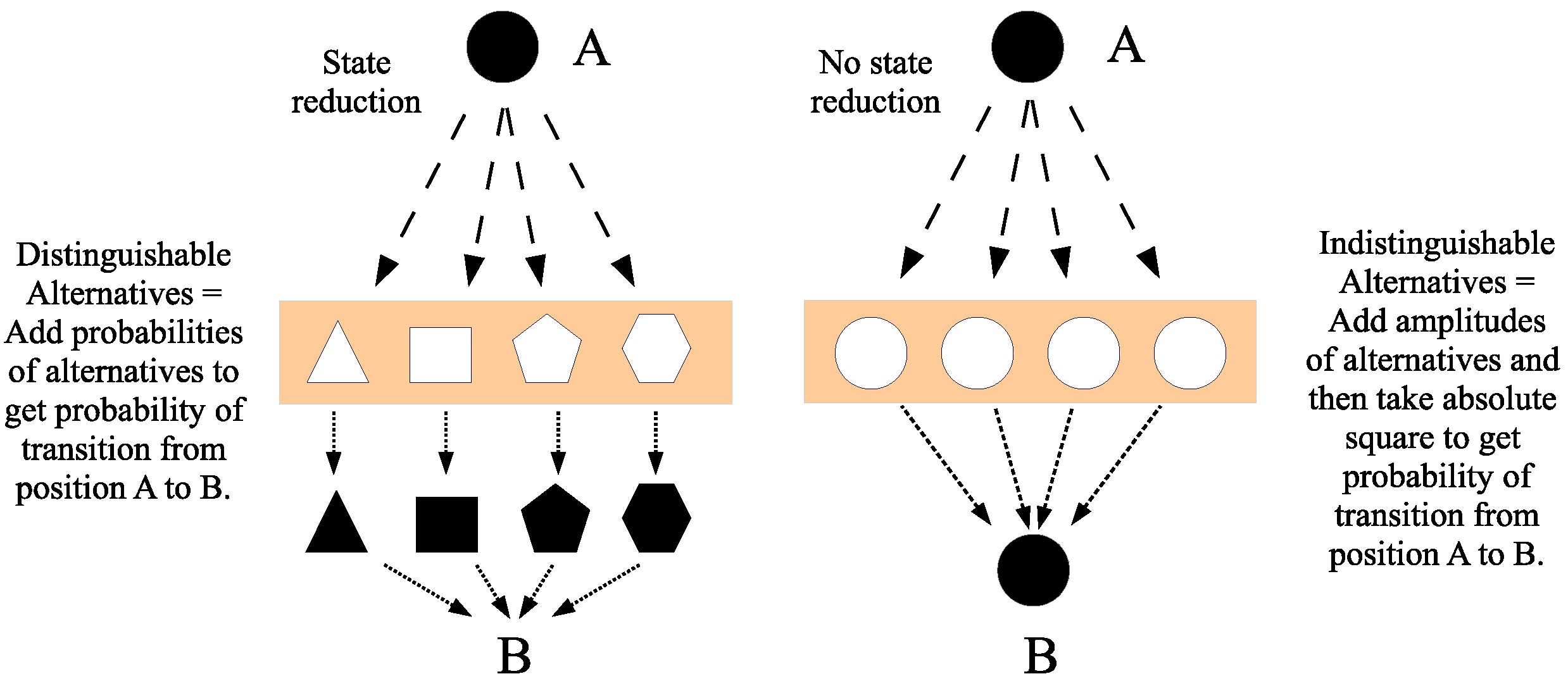
Hermann Weyl, in his informal writing about quantum mechanics, used the notion of a grating or sieve and implicitly used the Yoga to liken an equivalence relation on a set to a direct-sum decomposition of a vector space as two types of gratings [57] (p. 256). Then, a measurement of a state would be the application of a grating. In Figure 15, the grating metaphor for state reduction or measurement is used to illustrate the Feynman rules, where the ‘ball of dough’ black circle is like the superposition of the polygon-shapes, and when it passes through the distinguishing grating (left side of the figure), it reduces to one of the polygon shapes. On the right-side of the figure is the non-distinguishing grating so the amplitudes to go through each round hole are added to get the amplitude of going from A to B, and then the absolute square gives the probability.

Thus, the partitional analysis, in terms of making distinctions or not, is realized in the Feynman rules based on distinguishability or indistinguishability. In the two-slit experiment, case 1 is the distinguishable case (in Feynman’s terms), where there were detectors at the slits, and case 2 is the indistinguishable case, with no detectors at the slits. In Feynman’s example, the measurement is entirely at the quantum level with no macroscopic apparatus. Hence, the Feynman analysis undermines the approach trying to analyze measurement in term of the “decoherence” induced by a macroscopic measuring devices (e.g., [58]) as well as the literature about the “von Neumann cut” [49] (or “Heisenberg cut”) also involving macroscopic measuring devices. With virtual certainty that the state reductions take place at the quantum level, the literature about the ‘problems’ arising from extending Schrödinger’s equation to the macroscopic level (e.g., his eponymous cat) are pseudo-problems. Naturally, humans need some amplification of the quantum level physical result in the distinguishable case to know the result, but such macroscopic considerations have no role in quantum theory.

3.4.9. Summing up about Quantum Mechanics

Even though the Hermitian observables have real eigenvalues, quantum mechanics could not be formulated in vector spaces over the reals since the reals are not algebraically complete. Only in the algebraically complete extension of the reals, the complex numbers, could the Hermitian operators have a full set of eigenvectors [59] (p. 67, fn. 7). But the complex numbers are also the natural mathematics to express waves; in the polar representation, each complex number has an amplitude and a phase. But that turned out to be a major false clue about the nature of quantum reality. Now, it is widely accepted that the so-called “wave function” is only a computational device to compute probabilities by the Born rule, not a part of physical reality. Einstein’s famous quip that “The Lord is subtle, but not malicious” may need to be nuanced. If not malicious, He is at least a trickster. The mathematics of complex-valued vectors is not wrong, but it is certainly misleading if taken as a description of quantum reality.

That interpretive problem with waves was compounded by the misinterpretation of superposition, the key non-classical notion in QM. Superposition was misinterpreted as being like the classical addition of water waves or electromagnetic waves. Here, the approach by partitions or equivalence relations offered an alternative interpretation of superposition; the idea is that a superposition of definite states is indefinite on where the states differ and is only definite on commonalities. That is why superposition states are indefinite, blurry, blobby, or smeared-out, unlike the whole idea of superposition as the addition of physical waves. That basic wave-misinterpretation of superposition is compounded in the classroom ripple tank demonstration of the two-slit experiment. Again, it is not the math of complex numbers that is wrong but the interpretation of “probability waves” as matter waves like the water waves in a ripple tank. The partition approach was also helpful in building the pedagogical model of QM/Sets, which we used to model the two-slit experiment. In that model, using operations in a vector space over ${\mathbb{Z}}_2$, there was superposition and interference effects, but no waves.

The indefiniteness interpretation of superposition is certainly not new but it has been expressed in the language of “potentialities” by Werner Heisenberg [60], Abner Shimony [61], Gregg Jaeger [62], and many others, where indefinite states were described as being potentially any of a set of actualized definite states. But the notion of “potentiality” or “possibility” should be construed only as a manner of speaking (like “the thrown die has the potentiality of landing with six up”) instead of as a different ontological category of reality. There is only one type of reality but it can be in indefinite superposition states or definite eigenstates. Others, such as Henry Margenau [63] and R. I. G. Hughes [64], held similar views but used the word “latency” instead of “potentiality.” Many other quantum theorists have emphasized objective or ontic indefiniteness, such as Peter Mittelstaedt, “objective indeterminateness” [65] (p. 178), Paul Feyerabend, “inherent indefiniteness is a universal and objective property of matter” [66] (p. 202), and Fritz Rohrlich who saw “blurring as a fundamental ontic feature” [67] (p. 380). Thus, the partitional approach corroborates and clarifies this widespread acceptance of quantum reality as featuring objective indefiniteness. If quantum philosophers call any view of the nature of quantum reality an “interpretation”, then this might be called the “objective indefiniteness interpretation of quantum mechanics”.

4. Discussion and Conclusions

Our purpose has been to show that the subset–partitions duality (concretely, the elements and distinctions duality, and, abstractly, the reverse-the-arrows duality of category theory) shows up throughout the exact sciences in significant and sometimes unexpected ways, e.g., the connection between probability and information theory. But the major application has been to cast new light on the understanding and interpretation of quantum mechanics. Classical physics was very much a part of the Boolean worldview of full definiteness, and, thus, the dual worldview of partition logic and partition math turned out to play a major clarifying role in the century-old problem of interpreting quantum mechanics. The connection was simple: partitions or equivalence relations mathematically model the cohering together of states to become indefinite in partition blocks or equivalence classes; so, that clarifies at the set level the key non-classical notion in QM of superposition.

From these two basic ideas alone—indefiniteness and the superposition principle—it should be clear already that quantum mechanics conflicts sharply with common sense. If the quantum state of a system is a complete description of the system, then a quantity that has an indefinite value in that quantum state is objectively indefinite; its value is not merely unknown by the scientist who seeks to describe the system. … Classical physics did not conflict with common sense in these fundamental ways.

[68] (p. 47)

We have placed the partition math approach to understanding QM math in the context of the basic duality so that it will not be seen as another ad hoc, concocted, or jury-rigged attempt to make sense out of quantum mechanics, but as a natural application of the partition-side of the fundamental duality running throughout the exact sciences.

References

1. Ellerman, D. Partitions, Objective Indefiniteness, and Quantum Reality: The Objective Indefiniteness Interpretation of Quantum Mechanics; Springer Nature: Cham, Switzerland, 2024. [Google Scholar]
2. Boole, G. An Investigation of the Laws of Thought on Which Are Founded the Mathematical Theories of Logic and Probabilities; Macmillan and Co.: Cambridge, UK, 1854. [Google Scholar]
3. Church, A. Introduction to Mathematical Logic; Princeton University Press: Princeton, NJ, USA, 1956. [Google Scholar]
4. Mac Lane, S.; Moerdijk, I. Sheaves in Geometry and Logic: A First Introduction to Topos Theory; Springer: New York, NY, USA, 1992. [Google Scholar]
5. Birkhoff, G.; Von Neumann, J. The Logic of Quantum Mechanics. Ann. Math. 1936, 37, 823–843. [Google Scholar] [CrossRef]
6. Eilenberg, S.; Mac Lane, S. General Theory of Natural Equivalences. Trans. Am. Math. Soc. 1945, 58, 231–294. [Google Scholar] [CrossRef]
7. Lawvere, F.W.; Rosebrugh, R. Sets for Mathematics; Cambridge University Press: Cambridge, UK, 2003. [Google Scholar]
8. Finberg, D.; Mainetti, M.; Rota, G.-C. The Logic of Commuting Equivalence Relations. In Logic and Algebra; Ursini, A., Agliano, P., Eds.; Marcel Dekker: New York, NY, USA, 1996; pp. 69–96. [Google Scholar]
9. Britz, T.; Mainetti, M.; Pezzoli, L. Some operations on the family of equivalence relations. In Algebraic Combinatorics and Computer Science: A Tribute to Gian-Carlo Rota; Crapo, H., Senato, D., Eds.; Springer: Milano, Italy, 2001; pp. 445–459. [Google Scholar]
10. Ellerman, D. The Logic of Partitions: Introduction to the Dual of the Logic of Subsets. Rev. Symb. Log. 2010, 3, 287–350. [Google Scholar] [CrossRef]
11. Birkhoff, G. Lattice Theory; American Mathematical Society: New York, NY, USA, 1948. [Google Scholar]
12. Grätzer, G. General Lattice Theory, 2nd ed.; Birkhäuser: Boston, MA, USA, 2003. [Google Scholar]
13. Kung, J.P.S.; Rota, G.-C.; Yan, C.H. Combinatorics: The Rota Way; Cambridge University Press: New York, NY, USA, 2009. [Google Scholar]
14. Lawvere, F.W.; Schanuel, S. Conceptual Mathematics: A First Introduction to Categories; Cambridge University Press: New York, NY, USA, 1997. [Google Scholar]
15. Ellerman, D. The Logical Theory of Canonical Maps: The Elements & Distinctions Analysis of the Morphisms, Duality, Canonicity, and Universal Constructions in Set. arXiv 2022, arXiv:2104.08583. Available online: https://arxiv.org/abs/2104.08583 (accessed on 1 May 2024).
16. Rota, G.-C. Combinatorial Theory: The Guidi Notes; Guidi, J., Ed.; MIT Copy Services: Cambridge, MA, USA, 1998. [Google Scholar]
17. Rota, G.-C. Twelve problems in probability no one likes to bring up. In Algebraic Combinatorics and Computer Science: A Tribute to Gian-Carlo Rota; Crapo, H., Senato, D., Eds.; Springer: Milano, Italy, 2001; pp. 57–93. [Google Scholar]
18. Campbell, L.L. Entropy as a Measure. IEEE Trans. Inf. Theory 1965, IT-11, 112–114. [Google Scholar] [CrossRef]
19. Shannon, C.E. Some Topics in Information Theory. In Claude E. Shannon: Collected Papers; Sloane, N.J.A., Wyner, A.D., Eds.; IEEE Press: Piscataway, NJ, USA, 1993; pp. 458–459. [Google Scholar]
20. Shannon, C.E. A Mathematical Theory of Communication. Bell Syst. Tech. J. 1948, 27, 379–423, 623–656. [Google Scholar] [CrossRef]
21. Bateson, G. Mind and Nature: A Necessary Unity; Dutton: New York, NY, USA, 1979. [Google Scholar]
22. Collier, J. Information Originates in Symmetry Breaking. Symmetry Sci. Cult. 1996, 7, 247–256. [Google Scholar]
23. Muller, S.J. Asymmetry: The Foundation of Information; Springer: Berlin/Heidelberg, Germany, 2007. [Google Scholar]
24. Bennett, C.H. Quantum Information: Qubits and Quantum Error Correction. Int. J. Theor. Phys. 2003, 42, 153–176. [Google Scholar] [CrossRef]
25. Wilkins, J. Mercury or the Secret and Swift Messenger; John Nicholson: London, UK, 1708. [Google Scholar]
26. Gleick, J. The Information: A History, a Theory, a Flood; Pantheon: New York, NY, USA, 2011. [Google Scholar]
27. Gini, C. Variabilità e Mutabilità; Tipografia di Paolo Cuppini: Bologna, Italy, 1912. [Google Scholar]
28. Ellerman, D. New Foundations for Information Theory: Logical Entropy and Shannon Entropy; Springer Nature: Cham, Switzerland, 2021. [Google Scholar]
29. Rao, C.R. Gini-Simpson Index of Diversity: A Characterization, Generalization and Applications. Util. Math. B 1982, 21, 273–282. [Google Scholar]
30. Rao, C.R. Quadratic Entropy and Analysis of Diversity. Sankhyā Indian J. Stat. 2010, 72, 70–80. [Google Scholar] [CrossRef]
31. Martin, N.; England, J. Mathematical Theory of Entropy. Encyclopedia of Mathematics and Its Applications; Addison-Wesley: Reading, MA, USA, 1981; Volume 12. [Google Scholar]
32. Ainsworth, T. Form vs. Matter. In The Stanford Encyclopedia of Philosophy (Spring 2016 Edition); Zalta, E.N., Ed.; Stanford University: Stanford, CA, USA, 2016; Available online: https://plato.stanford.edu/archives/spr2016/entries/form-matter/ (accessed on 1 May 2024).
33. Heisenberg, W. Philosophic Problems of Nuclear Science; Fawcett Publications: Greenwich, CN, USA, 1952. [Google Scholar]
34. Pagels, H. Perfect Symmetry: The Search for the Beginning of Time; Simon and Schuster: New York, NY, USA, 1985. [Google Scholar]
35. Ariew, R. (Ed.) G. W. Leibniz and Samuel Clarke: Correspondence; Hackett: Indianapolis, IN, USA, 2000. [Google Scholar]
36. Kant, I. Critique of Pure Reason; Guyer, P.; Wood, A.W., Translators; Cambridge University Press: Cambridge, UK, 1998. [Google Scholar]
37. Weinberg, S. Dreams of a Final Theory; Vintage Books: New York, NY, USA, 1994. [Google Scholar]
38. Bunge, M. Matter and Mind: A Philosophical Inquiry. Boston Studies in the Philosophy of Science #287; Spring Publications: Dordrecht, The Netherlands, 2010. [Google Scholar]
39. Rota, G.-C. Indiscrete Thoughts; Birkhäuser: Boston, MA, USA, 1997. [Google Scholar]
40. Weinberg, S. Quantum Mechanics without State Vectors. Phys. Rev. A 2014, 90, 042102. [Google Scholar] [CrossRef]
41. Auletta, G.; Fortunato, M.; Parisi, G. Quantum Mechanics; Cambridge University Press: Cambridge, UK, 2009. [Google Scholar]
42. Lüders, G. Über Die Zustandsänderung Durch Meßprozeß. Ann. Phys. 1951, 8, 322–328. [Google Scholar] [CrossRef]
43. Furry, W.H. Some Aspects of the Quantum Theory of Measurement. In Lectures in Theoretical Physics; Brittin, W.E., Ed.; University of Colorado Press: Boulder, CO, USA, 1966; Volume 8A, pp. 1–64. [Google Scholar]
44. Ellerman, D. Quantum Mechanics over Sets: A Pedagogical Model with Non-Commutative finite Probability Theory as Its Quantum Probability Calculus. Synthese 2017, 194, 4863–4896. [Google Scholar] [CrossRef]
45. Feynman, R.P.; Leighton, R.B.; Sands, M. The Feynman Lectures on Physics: Quantum Mechanics; Addison-Wesley: Reading, MA, USA, 1965; Volume III. [Google Scholar]
46. Feynman, R.P. The Character of Physical Law; MIT Press: Cambridge, UK, 1967. [Google Scholar]
47. Leggett, A. Quantum Interview. In Elegance and Enigma: The Quantum Interviews; Schlosshauer, M., Ed.; Springer: Berlin/Heidelberg, Germany, 2011. [Google Scholar]
48. Dirac, P.A.M. The Principles of Quantum Mechanics, 4th ed.; Clarendon Press: Oxford, UK, 1958. [Google Scholar]
49. von Neumann, J. Mathematical Foundations of Quantum Mechanics; Beyer, R.T., Translator; Princeton University Press: Princeton, NJ, USA, 1955. [Google Scholar]
50. Stone, M.H. On One-Parameter Unitary Groups in Hilbert Space. Ann. Math. 1932, 33, 643–648. [Google Scholar] [CrossRef]
51. Norsen, T. Foundations of Quantum Mechanics; Springer International: Cham, Switzerland, 2017. [Google Scholar]
52. Feynman, R.P. The Concept of Probability in Quantum Mechanics. In Second Berkeley Symposium on Mathematical Statistics and Probability; University of California Press: Berkeley, CA, USA, 1951; pp. 533–541. [Google Scholar]
53. Stachel, J. Do Quanta Need a New Logic? In From Quarks to Quasars: Philosophical Problems of Modern Physics; Colodny, R.G., Ed.; University of Pittsburgh Press: Pittsburgh, PA, USA, 1986; pp. 229–347. [Google Scholar]
54. Zeilinger, A. Experiment and the Foundations of Quantum Physics. In More Things in Heaven and Earth; Bederson, B., Ed.; Springer: Berlin/Heidelberg, Germany, 1999; pp. 482–498. [Google Scholar]
55. Brukner, Č.; Zeilinger, A. Information and Fundamental Elements of the Structure of Quantum Theory. In Time, Quantum and Information; Castell, L., Ischebeck, O., Eds.; Springer: Berlin/Heidelberg, Germany, 2003; pp. 323–354. [Google Scholar]
56. Feynman, R.P.; Hibbs, A.R.; Styer, D.F. Quantum Mechanics and Path Integrals (Emended Ed.); Dover: Mineola, NY, USA, 2005. [Google Scholar]
57. Weyl, H. Philosophy of Mathematics and Natural Science; Princeton University Press: Princeton, NJ, USA, 1949. [Google Scholar]
58. Zurek, W.H. Decoherence, Einselection, and the Quantum Origins of the Classical. Rev. Mod. Phys. 2003, 75, 715–775. [Google Scholar] [CrossRef]
59. Weinberg, S. Lectures on Quantum Mechanics, 2nd ed.; Cambridge University Press: Cambridge, UK, 2015. [Google Scholar]
60. Heisenberg, W. Physics & Philosophy: The Revolution in Modern Science; Harper Torchbooks: New York, NY, USA, 1962. [Google Scholar]
61. Shimony, A. Search for a Naturalistic Worldview. Vol. II Natural Science and Metaphysics; Cambridge University Press: Cambridge, UK, 1993. [Google Scholar]
62. Jaeger, G. Quantum Objects: Non-Local Correlation, Causality and Objective Indefiniteness in the Quantum World; Springer: Berlin/Heidelberg, Germany, 2014. [Google Scholar]
63. Margenau, H. Advantages and Disadvantages of Various Interpretations of the Quantum Theory. Phys. Today 1954, 7, 6–13. [Google Scholar] [CrossRef]
64. Hughes, R.I.G. The Structure and Interpretation of Quantum Mechanics; Harvard University Press: Cambridge, MA, USA, 1989. [Google Scholar]
65. Mittelstaedt, P. The Constitution of Objects in Kant’s Philosophy and in Modern Physics. In Interpreting Bodies: Classical and Quantum Objects in Modern Physics; Castellani, E., Ed.; Princeton University Press: Princeton, NJ, USA, 1998; pp. 168–180. [Google Scholar]
66. Feyerabend, P. Problems of Microphysics. In Frontiers of Science and Philosophy; Colodny, R.G., Ed.; University Press of America: Lanham, MD, USA, 1983; pp. 189–283. [Google Scholar]
67. Rohrlich, F. Reality and Quantum Mechanics. In New Techniques and Ideas in Quantum Measurement Theory; Annals of the New York Academy of Sciences; Greenberger, D.M., Ed.; New York Academy of Sciences: New York, NY, USA, 1986; Volume 480, pp. 373–381. [Google Scholar]
68. Shimony, A. The Reality of the Quantum World. Sci. Am. 1988, 258, 46–53. [Google Scholar] [CrossRef]
Figure 1. Partition lattice on U = { a , b , c } .
Foundations 04 00013 g001
Figure 2. Venn diagram for compound logical entropies.
Foundations 04 00013 g002
Figure 3. Rooted tree illustrating the codes defined by a sequence of partition joins.
Foundations 04 00013 g003
Figure 4. Two creation stories described in terms of the elements and distinctions duality and the dual lattices.
Foundations 04 00013 g004
Figure 5. Boolean lattice of subsets of U = { a , b , c , d } .
Foundations 04 00013 g005
Figure 6. Lattice of partitions on U = { a , b , c , d } .
Foundations 04 00013 g006
Figure 7. Classical and quantum worlds illustrated using the lattice of partitions along with logical entropies.
Foundations 04 00013 g007
Figure 8. Partition join { { a , c } , { b } } { { a , b } , { c } } = 1 U .
Foundations 04 00013 g008
Figure 9. Setup for two-slit experiment.
Foundations 04 00013 g009
Figure 10. Case 1 probabilities at the detection wall.
Foundations 04 00013 g010
Figure 11. Case 1 state reductions to { a } or { c } and evolution to { a } or { c } , all at classical level.
Foundations 04 00013 g011
Figure 12. Case 2 probabilities at detection wall.
Foundations 04 00013 g012
Figure 13. Case 2 Evolution of the superposition { a , c } to { a , c } at the non-classical quantum level.
Foundations 04 00013 g013
Figure 14. Anschaulich (intuitive) picture of the two von Neumann processes.
Foundations 04 00013 g014
Figure 15. Grating metaphor illustrating the Feynman rule.
Foundations 04 00013 g015