Foundations of Nonequilibrium Statistical Mechanics in Extended State Space

Abstract

The review provides a pedagogical but comprehensive introduction to the foundations of a recently proposed statistical mechanics ($\mu$NEQT) of a stable nonequilibrium thermodynamic body, which may be either isolated or interacting. It is an extension of the well-established equilibrium statistical mechanics by considering microstates $\left\{{\mathfrak{m}}_k\right\}$ in an extended state space in which macrostates (obtained by ensemble averaging $\widehat{A}$) are uniquely specified so they share many properties of stable equilibrium macrostates. The extension requires an appropriate extended state space, three distinct infinitessimals $d_{\alpha }=(d,d_{\mathrm{e}},d_{\mathrm{i}})$ operating on various quantities q during a process, and the concept of reduction. The mechanical process quantities (no stochasticity) like macrowork are given by $\widehat{A}{d}_{\alpha }\mathsf{q}$, but the stochastic quantities ${\widehat{C}}_{\alpha }\mathsf{q}$ like macroheat emerge from the commutator ${\widehat{C}}_{\alpha }$ of $d_{\alpha }$ and $\widehat{A}$. Under the very common assumptions of quasi-additivity and quasi-independence, exchange microquantities $d_{\mathrm{e}}$q${}_k$ such as exchange microwork and microheat become nonfluctuating over $\left\{{\mathfrak{m}}_k\right\}$ as will be explained, a fact that does not seem to have been appreciated so far in diverse branches of modern statistical thermodynamics (fluctuation theorems, quantum thermodynamics, stochastic thermodynamics, etc.) that all use exchange quantities. In contrast, dq${}_k$ and $d_{\mathrm{i}}$q${}_k$ are always fluctuating. There is no analog of the first law for a microstate as the latter is a purely mechanical construct. The second law emerges as a consequence of the stability of the system, and cannot be violated unless stability is abandoned. There is also an important thermodynamic identity $d_{\mathrm{i}}Q\equiv d_{\mathrm{i}}W$$\ge 0$ with important physical implications as it generalizes the well-known result of Count Rumford and the Gouy-Stodola theorem of classical thermodynamics. The $\mu$NEQT has far-reaching consequences with new results, and presents a new understanding of thermodynamics even of an isolated system at the microstate level, which has been an unsolved problem. We end the review by applying it to three different problems of fundamental interest.

1. Introduction

Thermodynamics is the study of physical systems in nature that eventually evolve in time to stationary macrostates, in which any disturbance generates restoring forces to bring them back to the stationary macrostates [1,2,3], which makes them stable macrostates, usually called equilibrium (EQ) macrostate ${\mathfrak{M}}_{\mathrm{eq}}$, satisfying certain stability conditions. Any disturbance to modify macrostates of the system invariably results in nonequilibrium (NEQ) processes so that they abound in nature and obey the well-established second law [4,5,6,7]. The law is also obeyed by biological systems [8,9]. However, NEQ processes are not well-understood, as the corresponding thermodynamics (NEQT) is not yet fully developed, despite it having a long history of various competing schools [10,11,12,13,14,15,16,17,18,19,20,21,22,23,24,25,26,27,28], among which are the most widely known schools of local equilibrium thermodynamics, rational thermodynamics, extended thermodynamics, and GENERIC thermodynamics [21,29]. They mostly deal with the time evolution of macroscopic quantities only; the latter emerge as instantaneous averages over microstates in a more fundamental and statistical approach, and are used to characterize any thermodynamic process and the resulting nonnegative entropy generation ${\Delta }_{\mathrm{i}}S\ge 0$, as first proposed by Clausius [30,31]. In contrast, the equilibrium (EQ) thermodynamics (EQT) in which ${\Delta }_{\mathrm{i}}S\equiv 0$ is based on the original ideas of Carnot, Clapeyron, Clausius, Thomson, Maxwell, and many others [3,12,32,33,34,35,36,37,38,39,40,41,42,43,44,45], and has by now been firmly established in statistical physics, thanks to Boltzmann [46,47] and Gibbs [48], who established that classical EQ thermodynamics is a direct consequence of the EQ statistical mechanics [33,34,37,38] that deals directly with microstates $\left\{{\mathfrak{m}}_k\right\}$ of the Hamiltonian $\mathcal{H}$ of the system, and their equilibrium probabilities $\left\{p_k^{\mathrm{eq}}\right\}$ that together specify the EQ macrostate ${\mathfrak{M}}_{\mathrm{eq}}$. In contrast, EQT deals directly with ${\mathfrak{M}}_{\mathrm{eq}}$ without any need to know $\left\{{\mathfrak{m}}_k\right\}$ and $\left\{p_k^{\mathrm{eq}}\right\}$.

In general, the collection $\left\{{\mathfrak{m}}_k,p_k\right\}$ of microstates and their probabilities is used in a statistical description of a macrostate $\mathfrak{M}$ of the system $\Sigma$ that may be isolated or interacting with a medium $\tilde{\Sigma }$, as shown in Figure 1. The same microstate set $\left\{{\mathfrak{m}}_k\right\}$ determines different macrostates depending on the probabilities $p_k=p_k\left(\mathfrak{M}\right)$ with which ${\mathfrak{m}}_k$ appears in $\mathfrak{M}$. As $\mathcal{H}$ is by definition deterministic, ${\mathfrak{m}}_k$ is also deterministic. Thus, it is independent of $p_k$, but is specified by its energies $E_k$ and the parameters defining $\mathcal{H}$. Because of this, $\left\{{\mathfrak{m}}_k\right\}$ and $\left\{E_k\right\}$ are the same for any of its possible macrostates $\mathfrak{M}$ including ${\mathfrak{M}}_{\mathrm{eq}}$. This allows $\left\{E_k\right\}$ to be treated as purely mechanical, which is then supplemented by $\left\{p_k\right\}$ to add stochasticity to the mechanical system. Such a description has proven very useful in EQ statistical mechanics [33,34], where the concepts of the entropy $S_{\mathrm{eq}}=S\left({\mathfrak{M}}_{\mathrm{eq}}\right)$ that was first introduced by Clausius [30,31] as a state function of ${\mathfrak{M}}_{\mathrm{eq}}$, and the temperature T are the new concepts that play a central role in the resulting EQ thermodynamics of $\Sigma$. As such, it is very common to use them to distinguish a thermodynamic system from a mechanical system by recognizing that the concept of heat (a consequence of a particular commutator as described later) is novel to thermodynamics but is not applicable to a mechanical system, which is traditionally taken to be described by a purely conservative Hamiltonian $\mathcal{H}$. We use $\mathbf{X}\doteq (N,E,V,\cdots )$ to collectively denote the number of particles N, their energy E, the volume V occupied by them, etc., as representing the common thermodynamic extensive state variables that determine ${\mathfrak{M}}_{\mathrm{eq}}\equiv \mathfrak{M}\left(\mathbf{X}\right)$ in the state space ${\mathfrak{S}}_{\mathbf{X}}$ spanned by $\mathbf{X}$. We call them observables. As observables, these variables can be controlled from the outside of the system. We will allow $\mathbf{X}=\mathbf{X}\left(t\right)$ to have time dependence in this work; here, t denotes the time. For the moment, we suppress the suffix “eq” for notational simplicity unless necessary as we are dealing with ${\mathfrak{S}}_{\mathbf{X}}$. To be useful, S and T must uniquely refer to the thermodynamic state $\mathfrak{M}\left(\mathbf{X}\right)$. This unique relationship is what is meant by S being a state function of $\mathbf{X}$, which when inverted gives E a state function of $\zeta \doteq (S,\mathbf{w}),\mathbf{w}\doteq \mathbf{X}\setminus E$, where $\setminus E$ stands for deleting E from the set preceding it. Being functions of $\mathfrak{M}$ of $\Sigma$, S and T, an intensive field, must be interrelated in some fashion such as

$$1/T=\partial S/\partial E,$$

(1)

(see Equation (129)) so only one of them can be treated as a primitive concept, which we take to be the entropy. The goal of NEQT is to then specify it in terms of $\mathbf{X}$ in the state space ${\mathfrak{S}}_{\mathbf{X}}$. In this respect, having S a state function considerably simplifies the study as we then deal with ${\mathfrak{M}}_{\mathrm{eq}}$. When this cannot be done, we must go beyond ${\mathfrak{S}}_{\mathbf{X}}$ to an extended state space in which the NEQ entropy also becomes a state function, which is the central theme of this review. In this space, a uniform global temperature of the body is defined as its unique field by the above derivative in the extended state space. Thus, our goal will be to identify the NEQ entropy in this space.

Although S plays important roles in diverse fields ranging from classical thermodynamics of Clausius [3,10,12,13,17,20,24,25,30,33,39,40,41,42,43,44,46,47,48,49,50,51,52,53,54,55,56,57,58], quantum mechanics and uncertainty [59,60,61], black holes [62,63,64], coding and computation [65,66,67], to information technology [68,69,70,71,72], it does not seem to have a standard definition in all cases, even though it is well-defined under EQ conditions, as extensively discussed in the literature; see, for example, [46,47,48,73,74,75,76,77,78]. As $S_{\mathrm{eq}}$ is uniquely determined by $\left\{p_k^{\mathrm{eq}}\right\}$ as a state function, $p_k^{\mathrm{eq}}$’s must be unique functions in ${\mathfrak{S}}_{\mathbf{X}}$, as is well-known [33]. Requiring this uniqueness will be a guiding force in our endeavor to formulate the NEQ statistical mechanics. Whether S has any physical significance in a NEQ macrostate $\mathfrak{M}$ has been a topic of extensive debate; see for example [73,74,75,76,77] and references therein. The  problem arises because it is not clear if, and how, $\mathfrak{M}$ can be uniquely identified. Because of the lack of uniqueness, introducing $S\left(\mathfrak{M}\right)$ as a state function becomes nontrivial. The same concern also applies to $\left\{p_k\right\}$.

Recently, we have been able to extend the classical concept of Clausius entropy from EQ states to NEQ states where irreversible entropy is generated [75,76,77,78]. That approach is an outgrowth of an earlier review [79] in this journal about a possible source of stochasticity that is required in a thermodynamic system, even though its mechanics is completely deterministic due to its Hamiltonian dynamics so that heat and temperature have no mechanical analogs. Not appreciating that the source of stochasticity is independent from the deterministic (mechanical) aspect has been a source of bitter debate between Boltzmann, Zermelo, Poincare, and many others ([45,56,79,80,81,82,83,84,85,86,87,88,89,90,91,92,93,94,95,96], and references cited in there). The dispute required Boltzmann to propose the ideas of molecular chaos and of the ergodicity hypothesis [91] that have played a major role in EQ statistical mechanics. We discuss these important ansatze in [92,93,94,95] with an emphasis on Kac’s ring model [97,98] in more detail, where we find that they are not fulfilled in a deterministic dynamics. We infer, as is commonly believed, that one needs a stochastic dynamics for the ansatz to be satisfied. Both these ideas can only be supported by a stochastic dynamics as discussed in these references [99,100,101,102].

It is clear that we need to supplement a purely mechanical approach by supplementing it with stochasticity. We accomplish treating both aspects separately but unifying them together and enabling uniqueness by using an extended state space ${\mathfrak{S}}_{\mathbf{Z}}$ spanned by extensive state variables (compactly denoted by $\mathbf{Z}=\mathbf{Z}\left(t\right)=\mathbf{X}\left(t\right)\cup \xi \left(t\right)$ as an extension of $\mathbf{X}\left(t\right)$ in this review) to obtain a state function S. In general, $\mathbf{Z}$ includes the observables but possibly some more independent variables, compactly denoted by $\xi \left(t\right)$ required for an NEQ situation, as will become clear later. The additional state variable $\xi$, when properly chosen as will be described later, allows for a unique description of the macrostate $\mathfrak{M}\left(\mathbf{Z}\right)$ in ${\mathfrak{S}}_{\mathbf{Z}}$. Once such a state space has been uncovered for $\mathfrak{M}\left(\mathbf{Z}\right)$, its entropy $S\left(\mathfrak{M}\right)$ also become a state function$S\left(\mathbf{Z}\right)$ in ${\mathfrak{S}}_{\mathbf{Z}}$. This again requires its $p_k$’s to be unique functions in ${\mathfrak{S}}_{\mathbf{Z}}$, just as $p_k^{\mathrm{eq}}$ are in ${\mathfrak{S}}_{\mathbf{X}}$. Thus, the identification of an appropriate ${\mathfrak{S}}_{\mathbf{Z}}$ immediately solves the problem of obtaining a unique statistical mechanics of an NEQ system as it directly leads to $p_k$ as a unique function of ${\mathfrak{m}}_k$ and $\mathfrak{M}\left(\mathbf{Z}\right)$ in ${\mathfrak{S}}_{\mathbf{Z}}$.

In order for such an approach to work, and in particular for $S\left(\mathbf{Z}\right)$, which itself is a system quantity, it is crucial that we deal with only system-intrinsic (SI) quantities (they are determined by the system), and not medium-intrinsic (MI) quantities (they are primarily determined by the medium) for the simple reason that utilizing $\left\{{\mathfrak{m}}_k\right\}$ requires their specification by the Hamiltonian of the system and so require SI-quantities for its specification. (We will use body to refer to $\Sigma ,\tilde{\Sigma }$, and ${\Sigma }_0$, and BI-quantities to refer to quantities of a body.) As will become clear in the following, these quantities capture the internal processes going on within the system. They cannot be fully captured by the MI-quantities, even though they have been traditionally used in thermodynamics, for the simple reason that they retain the memory of the medium and can depend on the system only weakly. Thus, they will require additional steps to study internal processes. There has been a long debate about the relevance and significance of the two kinds of quantities that ensued from a very different perspective [103,104,105,106,107], but did not capture the importance these quantities acquire in our approach.

The SI-quantities allow us to develop our NEQ statistical mechanics, which for brevity is identified as the $\mu$NEQT, with $\mu$ referring to the microstates $\left\{{\mathfrak{m}}_k\right\}$, in which we directly capture internal processes that are responsible for irreversibility. As the collection $\left\{{\mathfrak{m}}_k\right\}$ is the central object in the $\mu$NEQT, the latter deals with quantities such as $\left\{E_k,p_k\right\}$. At the microstate level, there are fluctuations that are essential in a statistical treatment, and are properly captured in the $\mu$NEQT through the fluctuations in $E_k$ and $p_k$ over ${\mathfrak{m}}_k$. In contrast, the use of the MI-quantities does not directly describe $\left\{{\mathfrak{m}}_k\right\}$ so it cannot properly yield a statistical mechanical description of an NEQ process in a system. This is one of our most important conclusions. In particular, an important consequence of the $\mu$NEQT as will be shown later is that MI-quantities, after  reduction (being averaged over the microstates of the medium) under commonly accepted conditions of quasi-additivity and quasi-independence, do not exhibit any fluctuations. This explains why they are not suitable in developing the statistical mechanics. We call the resulting version of the microstate NEQT the $\mathring{\mu }$NEQT; the circle on $\mu$ is a reminder for the use of “exchange” microquantities derived from the MI-quantities in its formulation. The most prominent are the exchange (also called external) microwork $d_{\mathrm{e}}{W}_k=d_{\mathrm{e}}W,\forall k$, and the exchange (also called external) microheat $d_{\mathrm{e}}{Q}_k=d_{\mathrm{e}}Q,\forall k$, thus, explicitly exhibiting that they have no fluctuations. Because of this, it does not directly capture internal processes at the microstate level, which require additional steps to describe irreversibility as mentioned above. The  corresponding macroscopic NEQT from the two approaches are called the MNEQT and the $\mathring{\mathrm{M}}\mathrm{NEQT}$, respectively; here, M stands for the macroscopic description in terms of macrostates, the circle again having the same connotation as above. There are no fluctuations in these theories, as is well-known. The $\mathring{\mathrm{M}}\mathrm{NEQT}$ is the standard formulation of classical thermodynamics and has been discussed extensively by many prominent scientists [13,18,33,39,41,42,51,108], some including internal variables that play an important role in our approach.

It should be obvious from the above discussion that we need to make a clear distinction between fluctuating (Fl) and nonfluctuating (NFl) quantities. In  addition, we also recognize that there are many other macrostates in ${\mathfrak{S}}_{\mathbf{Z}}$ for which neither S nor the corresponding $p_k$’s are unique functions in ${\mathfrak{S}}_{\mathbf{Z}}$, so S must be treated independently of $\mathbf{Z}$. Our previous work did not consider such states, but they will be considered in this review. For this purpose, we will find it convenient to introduce the following state variable sets:

$$S,E,\mathbf{w}\doteq \mathbf{X}\setminus E,\mathbf{W}\doteq \mathbf{Z}\setminus E,\mathbf{Z},\zeta =(S,\mathbf{W}),\chi =(S,\mathbf{Z}),$$

(2)

and the corresponding state spaces ${\mathfrak{S}}_S,{\mathfrak{S}}_E,{\mathfrak{S}}_{\mathbf{W}},{\mathfrak{S}}_{\mathbf{Z}},{\mathfrak{S}}_{\zeta }\doteq {\mathfrak{S}}_S\cup {\mathfrak{S}}_{\mathbf{W}}$, and  ${\mathfrak{S}}_{\varnothing }\doteq {\mathfrak{S}}_S\cup {\mathfrak{S}}_{\mathbf{Z}}$, where the suffix denotes the variable set forming the state space.

We should emphasize that internal variables also appear in mechanical systems. A simple example is that of two particles in a system, whose interior is hidden in the lab from us so that we cannot see where the particles are inside the system. From outside the system, we can only be aware of the position of the center of mass by observing its motion in the lab. However, there is no way to determine their separation within the system. This separation and the corresponding relative motion are examples of the internal variable and its motion, and play a role in the dynamics of the mechanical system. Thus, it should not come as a surprise that such internal variables will also be relevant in a thermodynamic system. Indeed, we will see later in Section 14 that this relative motion becomes the source of “microfriction”, resulting in friction, when we treat the system in thermodynamics.

To appreciate at a more fundamental level the distinction between a mechanical and a thermodynamic system, we first realize that both systems are usually separated from their surroundings $\tilde{\Sigma }$ by some clear partitions, the most common being the walls between them; see Figure 1. We collectively call them containers or walls that contain the system [109]. In this review, we find it convenient to not include the container as part of the system, but use it to determine the boundary conditions for the equations of motion or as defining parameters in the Hamiltonian $\mathcal{H}$ of the system $\Sigma$. As $\mathcal{H}$ plays the role of E, the parameters $\mathbf{w}$ and $\mathbf{W}$ are obtained by taking out E from $\mathbf{X}$ and $\mathbf{Z}$, respectively:

$$\mathbf{w}=(V,\cdots ),\mathbf{W}=(V,\cdots ,\xi );$$

(3)

where ⋯ refers to the rest of the elements in $\mathbf{X}$ besides V [110]. As will become evident below, these parameters denote the work parameter in the Hamiltonian, which we will denote by $\mathcal{H}\left(\left.\mathbf{x}\right|\mathbf{w}\right)$ or $\mathcal{H}\left(\left.\mathbf{x}\right|\mathbf{W}\right)$, respectively. For simplicity in the following, we will always use $\mathbf{W}$ for the work parameter to refer to both cases and express the Hamiltonian as $\mathcal{H}\left(\left.\mathbf{x}\right|\mathbf{W}\right)$. The parameter can be varied in a process with a concomitant change in $\mathcal{H}\left(\left.\mathbf{x}\right|\mathbf{W}\right)$ due to the work done by the system. This is in accordance with the work–energy theorem of mechanics that states that the change in the energy is due to work alone. Also, $\mathbf{x}=\mathbf{x}\left(t\right)\doteq \left\{\mathbf{r}\left(t\right),\mathbf{p}\left(t\right)\right\}$ is the dynamical variable and denotes the collection of coordinates $\left\{\mathbf{r}\left(t\right)\right\}$ and momenta $\left\{\mathbf{p}\left(t\right)\right\}$ of the N particles in the phase space $\Gamma \left(\mathbf{x}\left|\mathbf{W}\right.\right)$ of $\Sigma$ [110]. As internal variables play no role in EQ, $\mathbf{W}=\mathbf{w}$ in EQ. For any $\mathbf{x}\in \Gamma \left(\mathbf{x}\left|\mathbf{W}\right.\right)$, the  deterministic energy of $\Sigma$ in the state specified by $\mathbf{x}$ is $E_{\mathbf{x}}\left(\mathbf{W}\right)=\mathcal{H}\left(\left.\mathbf{x}\right|\mathbf{W}\right)$, which need not be constant. However, there is no stochasticity so there is no concept of heat. Thus, the Hamiltonian itself cannot explain the fundamental difference between the two systems [79].

We elaborate further. Mechanics is a branch of the physical science to study the deterministic behavior of the system in the presence of known forces and radiation in time. The central concept is that of energy whose changes are governed by deterministic Hamiltonian equation of motion in $\Gamma \left(\mathbf{x}\left|\mathbf{w}\right.\right)$ with deterministic boundary conditions such as at the walls confining the system $\Sigma$ (see Figure 1a) that generate deterministic wall potentials acting on the particles. Accordingly, a point $\mathbf{x}\left(t\right)\in \Gamma \left(\mathbf{x}\left|\mathbf{w}\right.\right)$ is uniquely determined by $\mathbf{x}\left(t_0\right)$ at some reference time $t_0$. A central aspect of the equation is that it uniquely determines the properties of the system in the future ($t>t_0$) as well as in the past ($t<t_0$) [111,112]. We will assume in this review that the fundamental weak nuclear forces are not included in our discussion [113]. A movie of such a deterministic process in the future, when run backward for the past, will appear just as natural with no hint of the direction of the time flow. Thus, starting from $\mathbf{x}$, which also identifies a microstate [110], at  t, the state undergoes a unique state transformation

$$\mathbf{x}⟼{\mathbf{x}}^{\prime }$$

(4)

in the same interval $\Delta t$ for any $\Delta t$. If we now consider an ensemble of the same mechanical system, each prepared in the state $\mathbf{x}$ at $t=0$, then at $t=\Delta t$, each system will be in the same state ${\mathbf{x}}^{\prime }$. In the language of probability theory [114], we say that ${\mathbf{x}}^{\prime }$ follows with certainty from $\mathbf{x}$ in $\Delta t\gtrless 0$. (This will be useful later to associate the concept of a constant entropy to a mechanical system but not heat.)

But the above invariance is contrary to our daily experience as a rule [115,116,117,118,119,120,121,122,123,124]. For example, the initial state ${\mathbf{x}}_0$ may be when all the gas particles are confined to a small portion of the container [109] located at the center of the container. We are not interested in particle momenta. As the gas expands spontaneously, it occupies the entire volume uniformly. However, once the gas has occupied the entire volume in the state ${\mathbf{x}}_1$, the reverse evolution is not seen in nature. Similarly, the  cream mixed in a cup of coffee does not ever unmix on its own. The smoke from a burning piece of wood only spreads out in the room, but never confines itself on its own. If we run the movies in any of these cases backward, we immediately realize that the backward movies do not represent physical phenomena that are consistent with our daily experience.

This lack of time-reversal invariance of the equations of motion is a natural fact of daily life where we deal with macroscopic systems [125] that eventually evolve in time to ${\mathfrak{M}}_{\mathrm{eq}}$. This is at the root of the second law of thermodynamics, and can be easily explained as follows. It happens here that each member of the above ensemble that was initially prepared in the same state $\mathbf{x}$ evolves during a fixed interval $\Delta t$ into different states ${\mathbf{x}}^{\left(n\right)}={\mathbf{x}}^{\prime },$${\mathbf{x}}^{″},$$x^{‴}$$,\cdots$ for different $n=1,2,3,\cdots$

$$\mathbf{x}⟶{\mathbf{x}}^{\left(n\right)},n=1,2,3,\cdots ,$$

(5)

then the certainty implied in Equation (4) is lost so that most often it would happen that the states of different members after $\Delta t$ would have no discernible pattern for ${\mathbf{x}}^{\left(n\right)}$ and appear haphazard for the members. The result is ([126], pp. 1–14) a loss of physical determinism [127]. Thus, the mapping

$$\mathbf{x}⤏{\mathbf{x}}^{\prime }$$

(6)

in (5) between $\mathbf{x}$ and one of its evolved states ${\mathbf{x}}^{\prime }$ is one-to-many, and the mapping becomes unpredictable, i.e., stochastic [114]. One possible explanation of the loss of certainty at the level of states lies in the presence of stochasticity in the system due to the uncontrollable interactions with the surroundings, as discussed elsewhere [79] and elaborated later in Section 7. This is the foundations of classical probability theory by Laplace, and used to formulate the idea of density matrix by Landau [59,128] and von Neumann [129]. In this case, the mapping (6) cannot be reversed, and we cannot perform time-reversal of the evolution anymore. It is the success of a probabilistic approach to nonequilibrium thermodynamics that prompted Maxwell [50] and Boltzmann [130,131] to promote the “ergodic hypothesis” to achieve EQ. One of our aims in this review is to follow the consequences of this stochasticity in the dynamics such as in the Brownian motion [132] and Langevin’s equation [133], and  extend the concept of ergodicity to a special class of NEQ states [134] that has been identified as internal equilibrium states; see Definition 9.

1.1. Scope of the Review

It should be obvious that the scope of the NEQ statistical mechanics, the  $\mu$NEQT, is more general than that of the equilibrium statistical mechanics, to be denoted here simply as the $\mu$EQT in short, in that the attempts are now mostly to deal with the most general time evolution of microscopic quantities in the former. The instantaneous averages of these quantities over microstates $\left\{{\mathfrak{m}}_k\right\}$ are used to specify the instantaneous macrostates $\mathfrak{M}$ required to characterize any thermodynamic process$\mathcal{P}$ in time in the MNEQT. Thus, the tasks in the $\mu$NEQT and the MNEQT are more difficult and their foundations less developed, which justifies the motivation of this review. The exception is the validity of the first law in terms of exchange (or external) work and heat between $\Sigma$ and $\tilde{\Sigma }$ in thermodynamics, which plays a central role in the $\mathring{\mathrm{M}}\mathrm{NEQT}$. These MI-quantities are determined uniquely by $\tilde{\Sigma }$ regardless of $\mathcal{P}$ being reversible or irreversible, and are easily identified under generally acceptable conditions such as $\tilde{\Sigma }$ always being in EQ, quasi-additivity and quasi-independence; see later. Some of the approaches in the $\mathring{\mathrm{M}}\mathrm{NEQT}$ employ the enlarged state space ${\mathfrak{S}}_{\mathbf{Z}}$ [18,21,42,108]. Being associated with an EQ $\tilde{\Sigma }$, the MI-quantities including the exchange (or external) entropy carry no information about irreversibilities going on within the system. In contrast, the MNEQT based on the use of the SI-quantities include, by definition, these irreversible contributions so they are directly obtainable. One of our goals, besides laying down the foundations of the $\mu$NEQT, is to justify the MNEQT from the $\mu$NEQT.

A system in EQ always has its observables uniformly distributed throughout the system so it is uniform in ${\mathfrak{S}}_{\mathbf{X}}$ [33]. In  contrast, an NEQ system is not uniform and requires additional information about the nonuniformity to uniquely specify its states, which is provided by a proper choice of internal variables in $\xi$. The set $\xi$ allows us to treat $\Sigma$ as uniform in the state space ${\mathfrak{S}}_{\mathbf{Z}}$ (see Section 5.7) so that there is a unique thermodynamic temperature and other fields for the entire system even though it is still nonuniform in ${\mathfrak{S}}_{\mathbf{X}}$. This is very useful to obtain a proper thermodynamics of the system. For example, the  single thermodynamic temperature T even for a nonuniform system satisfies Clausius’s theorem that heat flows from hot to cold. This is what makes the $\mu$NEQT in the extended space ${\mathfrak{S}}_{\mathbf{Z}}$ so useful and desirable.

Various microquantities associated with $\Sigma$ (having microstates $\left\{{\mathfrak{m}}_k\right\}$), $\tilde{\Sigma }$ (having microstates $\left\{{\tilde{\mathfrak{m}}}_{\tilde{k}}\right\}$), and ${\Sigma }_0$ (having microstates $\left\{{\mathfrak{m}}_{0k_0}\right\}$) carry the suffix $k,\tilde{k}$, and $k_0$, respectively. However, we are only interested in microquantities associated with $\left\{{\mathfrak{m}}_k\right\}$ as our focus is on $\Sigma$. This means that microquantities of $\tilde{\Sigma }$ and ${\Sigma }_0$ must be manipulated so that they can be associated with $\left\{{\mathfrak{m}}_k\right\}$. To accomplish this, we introduce the principle of reduction, which accounts for the correlation introduced by mutual interactions between $\Sigma$ and $\tilde{\Sigma }$. Under commonly accepted conditions about $\tilde{\Sigma }$, the principle shows that the effect of $\tilde{\Sigma }$ on $\Sigma$ can be incorporated by treating its microquantities in the form of exchange (or external) quantities having no fluctuations. This is what makes the MI-quantities play such an important role in classical thermodynamics, but makes them unsuitable to extract fluctuations in a statistical theory.

Our goal here is to provide a comprehensive and self-contained introduction to our recently developed NEQ statistical mechanics ($\mu$NEQT), in which we study deterministic time evolution of individual microstates in $\left\{{\mathfrak{m}}_k\right\}$ along Hamiltonian trajectories in $\left\{{\gamma }_k\right\}$ during $\mathcal{P}$. When quantities associated with these trajectories are averaged over them using their probabilities, the result is the MNEQT, an extension of the equilibrium thermodynamics to describe NEQ processes. This consistency with the MNEQT is not only a check on the validity of the $\mu$NEQT, but also a justification of the MNEQT by the $\mu$NEQT. The use of the SI-quantities in the $\mu$NEQT allows for directly obtaining quantities such as ${\Delta }_{\mathrm{i}}S$ after averaging. Thus, the  $\mu$NEQT is an extension of the EQ statistical mechanics [33,34], the $\mu$EQT, that was originally developed by Boltzmann [46,47] and Gibbs [48], and limited to ${\Delta }_{\mathrm{i}}S\equiv 0$.

We will follow deterministic trajectories $\left\{{\gamma }_k\right\}$ during $\mathcal{P}$ between two macrostates ${\mathfrak{M}}_{\mathrm{in}}$ and ${\mathfrak{M}}_{\mathrm{fin}}$. Only the latter determine the trajectories so they are the same for all processes $\mathcal{P}$ between them. This makes $\left\{{\gamma }_k\right\}$ independent of the trajectory probabilities $\left\{p_{{\gamma }_k}\right\}$ controlling various $\mathcal{P}$’s, which is similar to $\left\{{\mathfrak{m}}_k\right\}$ being independent of the microstate probabilities $\left\{p_k\right\}$. The extended state space ${\mathfrak{S}}_{\mathbf{Z}}$ is chosen appropriately to uniquely specify $\left\{{\mathfrak{m}}_k\right\}$ and $\left\{{\gamma }_k\right\}$ in it. This uniqueness is an important aspect of the $\mu$NEQT and the MNEQT as it is missing in other contemporary NEQT theories [10,12,13,17,18,19,20,21,24,25,26,27,28,99,135,136,137,138,139,140,141,142,143,144,145,146,147]. The instantaneous $E_k$ along ${\gamma }_k$ can only change mechanically due to the variation in $\mathbf{W}$. This variation is responsible for the net change $\left\{\Delta E_k\right\}$ along $\left\{{\gamma }_k\right\}$, and is only determined by ${\mathfrak{M}}_{\mathrm{in}}$ and ${\mathfrak{M}}_{\mathrm{fin}}$ and not by $\left\{p_{{\gamma }_k}\right\}$ as noted above. To complete the formulation of the $\mu$NEQT, we determine the unique $\left\{p_{{\gamma }_k}\left(\mathcal{P}\right)\right\}$ for any $\mathcal{P}$ in ${\mathfrak{S}}_{\mathbf{Z}}$, which is another exceptional aspect of the $\mu$NEQT. This way, the deterministic aspect of a process (the mechanical work) has been separated from the stochastic aspect (the heat) in thermodynamics in a unique way in the $\mu$NEQT for any $\mathcal{P}$, NEQ or not. With the unique probabilities in hand, all calculation can be carried out exactly in the $\mu$NEQT, once ${\mathfrak{S}}_{\mathbf{Z}}$ has been identified. In the $\mathring{\mu }$NEQT, the trajectory probabilities need to be determined using additional steps such as using the master equation [54], Fokker–Planck equation [37,102], etc., which are phenomenological.

Being deterministic, microquantities associated with $\left\{{\mathfrak{m}}_k\right\}$ or $\left\{{\gamma }_k\right\}$ are not constrained by the second law, which is a macroscopic law based on stochasticity. This is not surprising, as the Hamiltonian dynamics has nothing to say about the second law. For the MNEQT, we need to determine various thermodynamic averages over $\left\{{\gamma }_k\right\}$ using $\left\{p_{{\gamma }_k}\right\}$. Thus, the development of the $\mu$NEQT is carried out in two independent stages. First we determine mechanical quantities as if the system is a mechanical one following Hamiltonian dynamics. Its stochastic aspects are captured by $\left\{p_{{\gamma }_k}\left(\mathcal{P}\right)\right\}$, which determine not only mechanical averages such as work but also the stochastic averages such as heat and entropy. It is the latter that finds itself manifested in the second law for appropriate choices of $\left\{p_k\right\}$ and $\left\{p_{{\gamma }_k}\right\}$. By simply modifying the second stage, we are able to investigate the catastrophic consequences of violating the second law. This proves the usefulness of our approach. With $\left\{\Delta E_k\right\}$ and $\left\{p_{{\gamma }_k}\left(\mathcal{P}\right)\right\}$ in hand, we now have a complete NEQ statistical mechanics to describe any process $\mathcal{P}$. The division in the two distinct and independent stages is of central importance to the $\mu$NEQT and the MNEQT [148,149,150,151,152,153,154,155,156,157].

We have successfully applied the $\mu$NEQT recently to study free expansion [154], to provide a correct application of microwork and microheat [155,156] in the various modern fluctuation theorems [26,158,159], and to describe viscous dissipation [157] associated with the dynamics of a Brownian particle (BP) [115,132,133,140] in its medium by developing an alternative to the stochastic Langevin description [38,99]. The above applications clearly show the usefulness of the $\mu$NEQT. However, our previous studies were mostly limited to microworks; microheats were not treated as extensively. One of our major incentives here is to overcome this limitation to determine the $\mu$NEQT for which the central requirement is the unique microstate probability $p_k$ in the state space ${\mathfrak{S}}_{\mathbf{Z}}$. This ensures that $\mathfrak{M}\left(\mathbf{Z}\right)$ and $S\left(\mathbf{Z}\right)$ are uniquely identified in ${\mathfrak{S}}_{\mathbf{Z}}$. Such macrostates are said to be in internal equilibrium (IEQ) in ${\mathfrak{S}}_{\mathbf{Z}}$ and written as ${\mathfrak{M}}_{\mathrm{ieq}}$ or $\mathfrak{M}\left(\mathbf{Z}\right)$, as opposed to EQ macrostates ${\mathfrak{M}}_{\mathrm{eq}}=\mathfrak{M}\left(\mathbf{X}\right)$ in ${\mathfrak{S}}_{\mathbf{X}}$. The  unique entropy $S\left(\mathbf{Z}\right)$ has the maximum possible value for a given $\mathbf{Z}$ so it has no memory of where the microstate has come from. Once $\mathfrak{M}$ becomes uniquely specified as $\mathfrak{M}\left(\mathbf{Z}\right)$ in ${\mathfrak{S}}_{\mathbf{Z}}$, it satisfies the extension of the ergodic hypothesis for ${\mathfrak{M}}_{\mathrm{ieq}}$; see Section 14 for an example.

But the applications so far of the $\mu$NEQT have provided only a piecewise and incomplete description of the $\mu$NEQT [148,149,150,151,152,153,154,155,156,157] that was restricted in scope to highlight its NEQ aspects in the limited context. This comprehensive review aims to overcome this limitation and provide a complete introduction to the foundation of the $\mu$NEQT by assimilating and extending together the previous results and by including missing details and newer aspects that emerge from the use of the SI-quantities in the extended state space ${\mathfrak{S}}_{\mathbf{Z}}$, where ${\mathfrak{m}}_k$ and $\mathfrak{M}$ are uniquely specified in an IEQ macrostate ${\mathfrak{M}}_{\mathrm{ieq}}$ just as they are uniquely specified for an EQ macrostate ${\mathfrak{M}}_{\mathrm{eq}}$ in the EQ state space ${\mathfrak{S}}_{\mathbf{X}}$. The $\mu$NEQT has met with success, as we will describe in this review, so it is desirable to introduce it to a wider class of readers.

Due to its microscopic SI-nature, the $\mu$NEQT provides a more detailed description of fluctuations in a thermodynamic process that are hidden in the MNEQT. For this reason, therefore, the former is highly desirable from both a theoretical and experimental point of view. It is an extension of the MNEQT [77,78,134,148,149,152,153,160] to the microstate level, which brings about a very close parallel with $\mu$EQT [32,33,34,36].

A microstate ${\mathfrak{m}}_k,k=1,2,\cdots$, carries an index k; the set $\left\{{\mathfrak{m}}_k\right\}$ forms a countable set and is specified by its energy set $\left\{E_k\left(\mathbf{W}\right)\right\}$; however, we will usually suppress $\mathbf{W}$ in ${\mathfrak{m}}_k$ and $E_k\left(\mathbf{W}\right)$, unless necessary. In a macrostate $\mathfrak{M}$, ${\mathfrak{m}}_k$’s appear with a probability $p_k\left(\mathfrak{M}\right)$; see Section 7 for details. For simplicity, we will also not explicitly show the argument $\mathfrak{M}$ in $p_k$; the dependence is always implicit. In the rest of the review, all quantities pertaining to $\mathfrak{M}$ are identified as macroquantities, while those pertaining to ${\mathfrak{m}}_k$ are identified as microquantities that always have the microstate index k of ${\mathfrak{m}}_k$ or of ${\mathbf{x}}_k$ in $\mathcal{H}\left(\left.{\mathbf{x}}_k\right|\mathbf{W}\right)$; see Definition 4. After statistical averaging over microstates using their probabilities $p_k$ (see Equation (12) for its proper definition), we obtain quantities without k or $\mathbf{x}$.

A microquantity associated with ${\mathfrak{m}}_k$ will always carry the index k (see later). A macrostate $\mathfrak{M}$ and a macroquantity associated with it do not carry the index k so it is always easy to distinguish the two kinds of quantities. We will continue to use “quantity” to stand for both microquantity and macroquantity, unless clarity is needed.

1.2. System-Intrinsic and Medium-Intrinsic Thermodynamics

As the medium is always taken to be in EQ, its properties do not change even if the system is out of equilibrium. This has made the choice of MI-description ($\mathring{\mathrm{M}}\mathrm{NEQT}$) very convenient to formulate classical thermodynamics [13,18,33,39,41,42,51,108], in which one uses the exchange macroheat ${\Delta }_{\mathrm{e}}Q=T_0{\Delta }_{\mathrm{e}}S$ in terms of the exchange entropy (see Equation (46)) and the exchange macrowork ${\Delta }_{\mathrm{e}}W$ (see Equation (135c)) such as ${\Delta }_{\mathrm{e}}W=P_0{\Delta }_{\mathrm{e}}V=P_0\Delta V$ for the PV-macrowork; see Equation (94) for the first law as an example. Here, $T_0$ and $P_0$ are the temperature and pressure of the medium (see Figure 1), which remain the same for all possible states of the system. This has made the $\mathring{\mathrm{M}}\mathrm{NEQT}$ a highly desirable thermodynamic theory as it is applicable in all cases. The main problem with this theory is that it is not directly applicable to an isolated system in Figure 1b for which exchange quantities are identically zero, but which provides the most cogent formulation of the second law $\Delta S_0\ge 0$; see Equation (213) in Proposition 3. It is useful only for an interacting system in Figure 1a for which the second law is stated indirectly in terms of irreversible entropy generation ${\Delta }_{\mathrm{i}}S\ge 0$; see Equation (67c). Indeed, all irreversible quantities including irreversible macrowork are indirectly determined.

In contrast, the MNEQT provides an SI-description involving quantities associated with the system alone so it is applicable to both systems in Figure 1 by explicitly taking into account the EQ properties of the medium, when it is present. All irreversible quantities including macroworks and macroheats are contained in this approach so they are determined directly in the MNEQT.

We elaborate on the distinction between the MNEQT and the $\mathring{\mathrm{M}}\mathrm{NEQT}$. The  exchange quantities $d_{\mathrm{e}}Z$ require the system $\Sigma$ to be embedded in a medium $\tilde{\Sigma }$ (see Figure 1a) and are controlled by $\tilde{\Sigma }$ [154] so that $d_{\mathrm{e}}Z=-d_{\mathrm{e}}\tilde{Z}$ (see Section 2) and  are easy to handle and measure, as $\tilde{\Sigma }$ is normally taken to be in equilibrium with no irreversibility ($d_{\mathrm{i}}\tilde{Z}=0$) so that $d_{\mathrm{e}}\tilde{Z}=d\tilde{Z}$. Thus, the exchange quantities do not directly provide any information about $d_{\mathrm{i}}Z$ and any irreversibility as mentioned above. As an example, the lost macrowork due to irreversibility in the $\mathring{\mathrm{M}}\mathrm{NEQT}$ is defined as

$${\mathring{d}}_{\mathrm{lost}}W={\mathring{d}}_{\mathrm{rev}}W-{\mathring{d}}_{\mathrm{irr}}W\ge 0,$$

where various ${\mathring{d}}_{\mathrm{rev}}W$ and ${\mathring{d}}_{\mathrm{irr}}W$ refer to the exchange macroworks along two distinct processes: a reversible and an irreversible. We have used a new notation $\mathring{d}$ to ensure that any $\mathring{d}W$ is not confused with $dW$ in the MNEQT. It is easy to see that ${\mathring{d}}_{\mathrm{lost}}W$ is precisely the irreversible macrowork $d_{\mathrm{i}}W$, which is determined by the actual process.

Similar distinctions can also be noted between the $\mathring{\mu }$NEQT and the $\mu$NEQT; they differ at least in the following important ways, with sweeping consequences, as we will see:

A.

The internal microwork ${\Delta }_{\mathrm{i}}{W}_k$ has no analog in the former because it uses the following questionable conjecture:

$${\Delta }_{\mathrm{e}}{W}_k\stackrel{?}{=}-\Delta E_k,$$

(7)

(see Section 15) which is often used in fluctuation theorems [99,135,136,137,138,139,140,141,142,143,144,145,146,147]; the use of $\stackrel{?}{=}$ is a reminder of its possible questionable nature, which is justified later in Theorem 7. In these fluctuation theorems, one begins with the conventional form of the first law $dE=d_{e}Q-d_{e}W$ in terms of exchange macroquantities, but identifies

$$d_{e}W\stackrel{?}{=}-{\sum }_k{p}_{k}d{E}_k,d_{e}Q\stackrel{?}{=}{\sum }_k{E}_{k}d{p}_k.$$

As a consequence of the above identification, no distinction can be made between fluctuating microwork

$$d{W}_k\equiv -d{E}_k,$$

which is an identity in accordance with the work–energy theorem (see Theorem 6) and nonfluctuating exchange microwork

$$d_e{W}_k=d_{e}W,\forall k;$$

see Theorem 7. The distinction is always maintained in the latter, in which we also show (see Section 10.1) why the above identification cannot be rigorously justified. Similar conclusions as above are obtained by replacing infinitesimal $d_{\alpha }$ by accumulation ${\Delta }_{\alpha }$, properly defined in Section 13 along a process $\mathcal{P}$.

B.

Consequently, the microforce imbalance ($\mu$FI) that results in fluctuating ${\Delta }_{\mathrm{i}}{W}_k=-{\Delta }_{\mathrm{i}}{E}_k$, a ubiquitous quantity, is absent in the former in that ${\Delta }_{\mathrm{i}}{W}_k=\Delta W_k-{\Delta }_{\mathrm{e}}{W}_k\equiv 0$ but is always present (${\Delta }_{\mathrm{i}}{W}_k\ne 0$) in the latter.

C.

The former results in a first law of thermodynamics ($\Delta E_k={\Delta }_{\mathrm{e}}{Q}_k-{\Delta }_{\mathrm{e}}{W}_k$) for each ${\mathfrak{m}}_k$, while the latter has it hold ($\Delta E={\Delta }_{\mathrm{e}}Q-{\Delta }_{\mathrm{e}}W$) only for a $\mathfrak{M}$; however, see Equation (243).

D.

The lost or dissipated macrowork ${\Delta }_{\mathrm{lost}}W$ measured by the average ${\Delta }_{\mathrm{i}}{W}_k$ should be absent in the former due to its above conjecture, but is always present in the latter.

E.

The exchange microwork ${\Delta }_{\mathrm{e}}{W}_k$ depends on the entire trajectory ${\gamma }_k$ in the former to make it fluctuating over ${\gamma }_k$, while in the latter, $\Delta W_k$ depends only on the terminal microstates of ${\gamma }_k$, and ${\Delta }_{\mathrm{e}}{W}_k\equiv {\Delta }_{\mathrm{e}}W$ is nonfluctuating (it is the same for all ${\gamma }_k$’s).

1.3. Main Results

The review emphasizes the very close parallel with EQ statistical mechanics ($\mu$EQT) that is clearly seen in the microstate probabilities and the existence of IEQ partition functions for ${\mathfrak{M}}_{\mathrm{ieq}}$. There are also major differences mainly in new concepts, some of which are very counter-intuitive, such as ubiquitous $d_{\mathrm{i}}{E}_k$, microforce imbalance ($\mu$FI) and internal microwork $d_{\mathrm{i}}{W}_k$ resulting from it, etc., for any macrostates including ${\mathfrak{M}}_{\mathrm{eq}}$ that have not been appreciated so far. They have been introduced previously [77,78,150,156,157] but now receive detailed explanation here. For example, it is a well-known fact that $d_{\mathrm{i}}E=0$ [12] (see Equation (53a)) for any $\mathfrak{M}$; yet $d_{\mathrm{i}}{E}_k$ is fluctuating and so can be different from zero, its average. The presentation here is simple enough to reach even an untrained reader. To accomplish this goal, we only focus on some examples borrowed from undergraduate physics so that a reader will not be lost; however, it does require an open mind to learn new concepts that are counter-intuitive and perplexing, as it is very hard to shake off old preconceptions.

Remark 1. 

As μEQT only deals with EQ processes, the second law plays no role here. However, the situation in the μNEQT is different, where we deal with NEQ processes. As the second law does not operate at the microstate level, our development of the μNEQT is not limited by this law. To make contact with thermodynamics, however, we will have to impose it at the level of macrostate. By investigating the internal inconsistencies that emerge if the second law is violated, we are able to conclude that the law cannot violated for a stable system. This is one of the most important benefits of our approach.

Throughout this review, we work in the enlarged state space ${\mathfrak{S}}_{\mathbf{Z}}$ so we include at least one internal variable $\xi$ as a prototype to make our discussion more realistic, as will become clear in Section 4 and Section 14. The main emphasis here will be to demonstrate the ubiquitous nature of internal changes such as $d_{\mathrm{i}}{E}_k$, a new concept whose existence has not been previously appreciated in various fluctuation theorems [26,158,159]. Not recognizing its existence has resulted in the conjecture $d_{\mathrm{e}}{W}_k=-d{E}_k=-$$d_{\mathrm{e}}{E}_k$ (see Equation (7)), used extensively in the $\mathring{\mu }$NEQT. This is contrary to a central result of the $\mu$NEQT; see Theorem 6. It is the microforce imbalance ($\mu$FI) between the internal and external microforces, a hitherto unrecognized purely mechanical concept at the microstate level in EQ and NEQ thermodynamics, that generates $d_{\mathrm{i}}{E}_k$ and is present in all processes, whether they are thermodynamic or not, as we will demonstrate. This is the most important outcome of the our approach; see Proposition 2. It emphasizes the importance of SI-quantities (such as in $d{E}_k=-d{W}_k$) that are very different from the MI-quantities (such as in $d_{\mathrm{e}}{E}_k=d{\tilde{W}}_k$) for any ${\gamma }_k$, even if the trajectory belongs to a reversible process. The use of generalized work $dW=-d{E}_{\mathrm{m}}$ in Equation (234a) as isentropic change allows us to calculate microscopic work (microwork) $d{W}_k$, which changes $E_k$ but not $p_k$. This is because ${\mathfrak{m}}_k$, whose concept is independent of $p_k$, uniquely determines $E_k$ for a fixed work set $\mathbf{W}$; see Definition 5. Therefore, $d{E}_k$ is uniquely determined by $d\mathbf{W}$ and does not have any contribution from the change in $p_k$. On the other hand, the generalized heat $dQ$ allows us to introduce microscopic heat (microheat) $d{Q}_k$, which does not change $E_k$ but changes $p_k$. The above mutually exclusive nature of $d{W}_k$ and $d{Q}_k$ proves to be a great simplification and allows us to treat $d{W}_k$ and $d{Q}_k$ as purely a mechanical and a stochastic concept, respectively, in the development of the $\mu$NEQT. In addition, as $d{E}_k$ does not have any contribution from $d{p}_k$, it has no microheat contribution, so there is no first law for ${\mathfrak{m}}_k$ in the $\mu$NEQT.

As $E_k$ is fluctuating, $d{E}_k=-d{W}_k$ is also fluctuating and is uniquely determined as $d{E}_k\doteq E_k(\mathbf{W}+d\mathbf{W})-E_k\left(\mathbf{W}\right)$ for ${\mathfrak{m}}_k$; the (slow or fast) nature of the process is irrelevant. The latter only controls $p_k$. This provides a simplification in evaluating the cumulative change $\Delta W_k$, which is independent of the nature of $\mathcal{P}$ between two macrostates; see Remark 71 and the discussion following it. The  fluctuating microwork $d{W}_k$ is different from $\Delta {\tilde{W}}_k=\Delta \tilde{W}$, which is the microwork done by the working medium on ${\mathfrak{m}}_k$ after reduction, and which depends strongly on the nature of $\mathcal{P}$ but is the same for all microstates for a given $\mathcal{P}$.

The most important new results that emerge in the $\mu$NEQT are the following:

• a clear separation of different kinds of work and heat and their fluctuations that emerge from $d_{\alpha }$;
• additional thermodynamic forces for irreversibility due to internal variables;
• stochasticity resulting from a nonvanishing commutator ${\widehat{C}}_{\alpha }\doteq d_{\alpha }\widehat{A}-\widehat{A}{d}_{\alpha }$;
• exchange microquantities are nonfluctuating, which makes them useless for directly obtaining fluctuations and irreversibility;
• the fundamental identity ${\Delta }_{\mathrm{i}}W={\Delta }_{\mathrm{i}}Q$ between irreversible macrowork and macroheat generalizing the result of Count Rumford and the Gouy-Stodola theorem;
• the origin of work dissipation ${\Delta }_{\mathrm{i}}W>0$ in an irreversible process;
• the uniqueness of macrostates and microstate probabilities in the enlarged state space for $\mathfrak{M}\left(\mathbf{Z}\right)$ determined by the experimental setup;
• the $\mu$NEQT justifies the MNEQT as the $\mu$EQT justifies the EQT.

1.4. Layout

The layout of the paper is the following. In the next section, we introduce our notation, definitions, and new concepts, which may be unfamiliar to many readers but are justified in the following sections. We describe here our basic approach that a thermodynamic description is equivalent to treating microquantities as purely mechanical without any consideration of stochasticity, to be followed by bringing in microstate probabilities to determine macroquantities, just as in EQ statistical mechanics. Microstate probabilities are not truly microquantities as they are not independent of each other. The stochasticity adds the dimension of entropy, without which we only have a mechanical description of an NEQ body in ${\mathfrak{S}}_{\mathbf{Z}}$. An arbitrary macrostate ${\mathfrak{M}}_{\mathrm{arb}}$ is divided into an EQ macrostate ${\mathfrak{M}}_{\mathrm{eq}}$ and an NEQ macrostate ${\mathfrak{M}}_{\mathrm{neq}}$; the latter is further divided into an IEQ (internal equilibrium) macrostate ${\mathfrak{M}}_{\mathrm{ieq}}$ and an NIEQ (non-internal equilibrium) macrostate ${\mathfrak{M}}_{\mathrm{nieq}}$. The IEQ macrostates share all the properties of EQ macrostates, except that the former have nonvanishing irreversible entropy generation ${\Delta }_{\mathrm{i}}S>0$. The principle of reduction is also introduced here. In Section 3, we discuss the mathematical properties of and manipulations with the linear operators $d_{\alpha }$, and give some examples for clarification. The origin of internal variables is explained in Section 4, where we show that they also emerge in mechanical descriptions so that they are not unique to thermodynamics. This explains why we need the enlarged state space ${\mathfrak{S}}_{\mathbf{Z}}$ for microscopic mechanical descriptions as well. We finally present the fundamentals of the $\mu$NEQT in Section 5. This is a very important section, where we present various axioms and requirements of the $\mu$NEQT. We then discuss stochasticity to derive a very general formulation of the entropy in terms of $\left\{p_k\right\}$, which is then used to obtain the unique form of $\left\{p_k\right\}$ for ${\mathfrak{M}}_{\mathrm{ieq}}$. An important and surprising aspect of the $\mu$NEQT is obtained in the equality of internal microwork (a mechanical microquantity) and microheat (a stochastic microquantity) even though they have distinct origins. At this stage, we have a complete and unique NEQ statistical mechanics (the $\mu$NEQT) in ${\mathfrak{S}}_{\mathbf{Z}}$. We identify SI-macroquantities and use them to derive the MNEQT for ${\mathfrak{M}}_{\mathrm{ieq}}$ exemplified by the Gibbs fundamental relation in ${\mathfrak{S}}_{\mathbf{Z}}$, which is then generalized to obtain the Gibbs fundamental relations for ${\mathfrak{M}}_{\mathrm{nieq}}$ in ${\mathfrak{S}}_{\mathbf{Z}}$.

In Section 6 and Section 7, we begin to introduce the mechanical and stochastic aspects of the $\mu$NEQT, respectively. In Section 6, we use $\mathbf{W}$ to identify microforces that operate in the mechanical formulation of the body so they are also present in its thermodynamic formulation. We use them to introduce the concept of microforce imbalance in Section 6.4, which captures the mechanical disparity between $\Sigma$ and $\tilde{\Sigma }$. The imbalance is responsible for the internal microwork. In Section 6.5, we derive the extension of the work–energy theorem of mechanics in ${\mathfrak{S}}_{\mathbf{Z}}$. In Section 7, we revisit a previous proposal for the origin of stochasticity and extend it further by discussing the effect of correlations between $\Sigma$ and $\tilde{\Sigma }$, and introducing the principle of reduction in Section 7.2. We then discuss quasi-independence in Section 7.3, and the simplification it brings about in thermodynamic considerations after reduction, especially with respect to the effects produced by $\tilde{\Sigma }$ on $\Sigma$, which is discussed in Section 7.4 and Section 7.5. The discussion, which forms a very important part of the review, shows why classical thermodynamics works so well.

In Section 8, we discuss the properties of the unique entropy $S_{\mathrm{ieq}}$ for ${\mathfrak{M}}_{\mathrm{ieq}}$ in ${\mathfrak{S}}_{\mathbf{Z}}$, and discuss its approximate formulation as a flat distribution that is commonly used in EQ statistical mechanics. This distribution neglects any fluctuations in the entropy, which are always present in the body. Despite this, it correctly gives the entropy so it can always be used to determine it as it simplifies the calculation. We show that the entropy additivity requires quasi-independence in Section 8.1 so the latter should not be confused with the principle of additivity for $\mathbf{W}$. Using this flat distribution, we provide a simple proof of the second law for ${\mathfrak{M}}_{\mathrm{ieq}}$ in ${\mathfrak{S}}_{\mathbf{Z}}$ in Section 8.3 by simply counting the number of distinct microstates as the system evolves in time, which can only increase with time; see Theorem 8. This direct proof is supplemented by Theorem 9 in Section 8.4 that the law is simply a direct consequence of the stability of the system so it does not need to be included as an additional part of Axiom 2 in the $\mu$NEQT; see Section 5). In Section 9, we show that a violation [161] of the second law results in internally inconsistent thermodynamics for stable physical systems, and cannot be taken seriously (see Conclusion 7), even though thermodynamic instabilities arise in approximate calculations such as van der Waals equations or mean field, but are always removed from consideration; see Remark 58. Therefore, we will always assume that we are dealing with a stable system for which the law is always valid, as noted in Section 1, except in Section 9. In Section 10, we initiate the formulation of the $\mu$NEQT by focusing on the two most important concepts, those of generalized or BI-microwork and microheat for ${\Sigma }_{\mathrm{b}}$. We show that various micro- and macroheats emerge from the nonvanishing commutator ${\widehat{C}}_{\alpha }$ introduced in Equation (229). For a fuller understanding, we first revisit in Section 10.1 the ensemble average of a fluctuating state variable, and its change in a process $\mathcal{P}$. We show that for $Z\in \mathbf{Z}$ such as E belonging to ${\mathfrak{S}}_{\mathbf{Z}}$, its change $dZ$ consists of two independent process contributions in orthogonal state spaces ${\mathfrak{S}}_{\mathbf{Z}}$ and ${\mathfrak{S}}_S$, a mechanical one $d{Z}_{\mathrm{m}}$ at fixed $\left\{p_k\right\}$ in ${\mathfrak{S}}_{\mathbf{Z}}$, and a stochastic one $d{Z}_{\mathrm{s}}$ at fixed $\left\{Z_k\right\}$ in ${\mathfrak{S}}_S$. Thus, $dZ\doteq d〈Z〉\in {\mathfrak{S}}_{\chi }$. In contrast, the stochastic state variable $S\in {\mathfrak{S}}_S$ has only stochastic contributions belonging to ${\mathfrak{S}}_S$. For E, $d{E}_{\mathrm{m}}$ represents the negative of the generalized macrowork $dW$, and $d{E}_{\mathrm{s}}$ the generalized macroheat $dQ$ in the body. Their statistical interpretation is covered in Section 10.2, where we show that $d{W}_k$ is purely mechanical, and $d{Q}_k$ purely stochastic. In Section 11, we discuss how $d_{\mathrm{e}}{p}_k$ and $d_{\mathrm{i}}{p}_k$ are determined, and how they determine the forms of various microworks, microheats, and microentropies. We also give a general proof of the identity $d_{\mathrm{i}}E\equiv 0$, even if $d_{\mathrm{i}}{E}_k\ne 0,\forall k$. This now completes the formulation of the unique NEQ statistical mechanics ($\mu$NEQT) in ${\mathfrak{S}}_{\mathbf{Z}}$.

The only thing remaining for a complete formulation of the $\mu$NEQT is to identify the choice of ${\mathfrak{S}}_{\mathbf{Z}}$, which is discussed in Section 12. This is a very important section that describes how the choice of ${\mathfrak{S}}_{\mathbf{Z}}$ is dictated by the way an experiment is performed, which must not come as a surprise for an NEQ process. This is because the observation and relaxation times play important roles here. By ordering various internal variables with their relaxation times in decreasing order, we show that only those internal variables have to considered whose relaxation times are greater than the observation time to uniquely specify the macrostate in ${\mathfrak{S}}_{\mathbf{Z}}$. We show how the unique microstate probability is identified. We consider the possibilities of fluctuating (Fl) and nonfluctuating (NFl) work parameter $\mathbf{W}$. It will be convenient to take the parameters to be fixed so that they are the same for all microstates. We introduce the Legendre transform $E_k^{\mathrm{L}}$ of the microenergy $E_k$, which proves to be very useful in expressing $p_k$. The discussion justifies that once ${\mathfrak{S}}_{\mathbf{Z}}$ has been identified in which $\mathfrak{M}$ becomes uniquely specified, the microstate probabilities are also uniquely specified. No auxiliary step is required to determine $p_k$. This is what makes the $\mu$NEQT so useful. The discussion is easily extended to consider a microstate that is not unique in ${\mathfrak{S}}_{\mathbf{Z}}$.

So far, we have provided a complete formulation of the $\mu$NEQT for any ${\mathfrak{M}}_{\mathrm{arb}}$ at each instant. To proceed further to extend the $\mu$NEQT for any process, we need to introduce a trajectory ensemble and determination of various path and process quantities, which is taken over in Section 13. We show that different trajectory quantities have different trajectory probabilities (path microprobabilities), which has not been appreciated so far. This finally provides a complete description of the $\mu$NEQT for any process.

We now turn to some of the applications of the $\mu$NEQT in the next three sections. In Section 14, we use it to describe the origin of microfricton at the microstate level. A new NEQ work fluctuation theorem is derived in Section 15 between any two arbitrary macrostates. In Section 16, we use the $\mu$NEQT to study the quantum and classical free expansion using our work fluctuation theorem. The final section provides a brief discussion of our conclusions and a summary.

2. Notation, Definitions and New Concepts

Before proceeding further, it is useful to introduce in this section our notation to describe various systems and their behavior, and new concepts for their understanding without much or any explanation (that will be offered later in the review where we discuss them). We also give various definitions and briefly discuss new concepts such as various forms of NEQ work and heat that need to be carefully distinguished for a precise formulation of the $\mu$NEQT. Various important concepts are highlighted in the form of Remarks to draw the attention of the reader. It is the hope that a reader can always come back here to be refreshed in case of confusion. In this sense, this section plays an important role in the review for the purpose of bookkeeping.

2.1. Systems and State Variables

Definition 1. 

A system Σ is a collection of material particles and radiation enclosed in a region of space defined by some parameter $\mathbf{W}$, and its Hamiltonian dynamics is determined by the Hamiltonian $\mathcal{H}\left(\mathbf{x}\left|\mathbf{W}\right.\right)$. A system can be embedded in a medium $\tilde{\Sigma }$, which is extremely large compared to it, and with which it interacts. The combined system ${\Sigma }_0$ formed by Σ and $\tilde{\Sigma }$ is commonly treated as an isolated system.

Remark 2. 

For convenience, we take the parameter $\mathbf{W}$ to be fixed so that it is the same for all microstates, even though it is not hard to take it to be unfixed so that it changes over the microstates. We will refer to them as nonfluctuating and fluctuating, respectively.

We draw attention to Figure 1 to introduce the notation. The  review mostly deals with statistical mechanics of macroscopically large systems $\Sigma$; however, we will also digress a bit to discuss small systems. In both cases, $\Sigma$ is extremely small compared to the medium $\tilde{\Sigma }$; see Figure 1b. The medium $\tilde{\Sigma }$ consists of two parts: a work source ${\tilde{\Sigma }}_{\mathrm{w}}$ and a heat source ${\tilde{\Sigma }}_{\mathrm{h}}$, both of which can interact with $\Sigma$ directly but not with each other. This separation allows us to study work and heat exchanges between $\Sigma$ and $\tilde{\Sigma }$ separately. We will continue to use $\tilde{\Sigma }={\tilde{\Sigma }}_{\mathrm{w}}\cup {\tilde{\Sigma }}_{\mathrm{h}}$ to refer to both of them together. The collection ${\Sigma }_0=\Sigma \cup \tilde{\Sigma }$ forms an isolated system, which we assume to be stationary. We remark that the concept of an isolated system in a laboratory is an important approximation [79,162] but extremely useful as no such system locally exists in reality. We need to always keep this in mind.

The system in Figure 1a is an isolated system, which we may not be able to divide into a medium and a system. Each medium in Figure 2, although not interacting with each other, has a similar relationship with $\Sigma$. In case they were mutually interacting, they can be treated as a single medium. The collection ${\Sigma }_0=\Sigma \cup {\tilde{\Sigma }}_1\cup {\tilde{\Sigma }}_2$ forms an isolated system. In the following, we will mostly focus on Figure 1 to introduce the notation, which can be easily extended to Figure 2 or to an extension with several mediums.

Definition 2. 

Observables $\mathbf{X}=(E,V,N,\cdots )$ of a system are extensive quantities that can be controlled from outside the system, and internal variables  $\xi =({\xi }_1,{\xi }_2,{\xi }_3,\cdots )$ are extensive quantities that cannot be controlled from outside the system. Their collection $\mathbf{Z}=\mathbf{X}\cup \xi$ is called the set of extensive state variables of Σ forming ${\mathfrak{S}}_{\mathbf{Z}}$, which we may simply write as $\mathfrak{S}$ when no confusion will arise. The set $\mathbf{W}$ or a subset of it may be fixed or may fluctuate over all microstates of Σ.

Definition 3. 

A system-intrinsic (SI) quantity is a quantity that pertains to the system Σ alone and can be used to characterize the system. A medium-intrinsic (MI) quantity is a quantity that is determined by the medium $\tilde{\Sigma }$ alone and can be used to characterize it and also the exchanges between Σ and $\tilde{\Sigma }$. No external exchange is allowed for ${\Sigma }_0$.

We use a suffix 0 to denote all quantities pertaining to ${\Sigma }_0$, a tilde $\left(\tilde{}\right)$ for all quantities pertaining to $\tilde{\Sigma }$, and no suffix for all quantities pertaining to $\Sigma$, even if it is isolated. Thus, the set of observables is denoted by ${\mathbf{X}}_0,\tilde{\mathbf{X}}$, and $\mathbf{X}$, respectively, and the set of state variables by ${\mathbf{Z}}_0,\tilde{\mathbf{Z}}$, and $\mathbf{Z}$, respectively, in the state space ${\mathfrak{S}}_{\mathbf{Z}}$; the set of internal variables are ${\xi }_0,\tilde{\xi }$, and $\xi$, respectively.

Remark 3. 

We will use the term “body” to refer to any of  $\Sigma ,\tilde{\Sigma },$ and ${\Sigma }_0$ in this review and use ${\Sigma }_b$ to denote it. However, to avoid notational complication, we will use the notation suitable for Σ for ${\Sigma }_b$ if no confusion would arise in the context. The mechanical aspect of a body is described by its Hamiltonian $\mathcal{H}\left(\left.\mathbf{x}\right|\mathbf{W}\right)$, and we refer to all quantities pertaining to it as body-intrinsic (BI), which includes SI, MI, and ISI (for the isolated system) as the case may be.

The discussion below is mostly for a body ${\Sigma }_{\mathrm{b}}$, but the notation is suited for a system. Thus, it covers the three systems $\Sigma ,\tilde{\Sigma }$, and ${\Sigma }_0$, unless mentioned otherwise.

Definition 4. 

A microstate of $\mathcal{H}\left(\mathbf{x}\left|\mathbf{W}\right.\right)$ represents the instantaneous deterministic state of ${\Sigma }_b$. The quantum microstates are specified by a set of good quantum numbers, which we usually denote by k as a single quantum number for simplicity; we take $k\in \mathbb{N},\mathbb{N}$ denoting the set of natural numbers. In the classical case, we use a small cell $\delta {\mathbf{x}}_k$ of volume $h^{3N}$ around ${\mathbf{x}}_k=\mathbf{x}$ as the microstate ${\mathfrak{m}}_k$ [163]; the collection $\left\{\delta {\mathbf{x}}_k\right\}$ covers the entire phase space Γ. A microstate ${\mathfrak{m}}_k$ appears with probability $p_k$ that is central for statistical mechanics.

Below, we clarify the definition further.

2.2. Microstates and Macrostates

Remark 4. 

In order to obtain a microscopic understanding of thermodynamics, we need to focus on the countable set of microstates ${\left\{{\mathfrak{m}}_k\right\}}_{k=1,2,\cdots }$. Then

$$E_k=\mathcal{H}\left(\left.{\mathbf{x}}_k\right|\mathbf{W}\right)$$

(8)

denotes the microenergy of ${\mathfrak{m}}_k$. In explicit form, the microenergy for ${\mathfrak{m}}_k$ of Σ will be expressed as $E_k\left(\mathbf{W}\right)$, for ${\tilde{\mathfrak{m}}}_{\tilde{k}}$ of $\tilde{\Sigma }$ it will be expressed as ${\tilde{E}}_{\tilde{k}}\left(\tilde{\mathbf{w}}\right)$ (see Equation (28a)), and for ${\mathfrak{m}}_{0k_0}$ of ${\Sigma }_0$ it will be expressed as $E_{0k_0}(\mathbf{W},\tilde{\mathbf{w}})$ (see Equation (28b)).

Remark 5. 

For clarity and ease of presentation, we will assume each microstate to be nondegenerate, i.e., a singlet. Extending the discussion to degenerate microstates is trivial, as discussed in Section 15.

We now identify microstates $\left\{{\mathfrak{m}}_k\right\}$. In quantum mechanics, they refer to the countable microstates of the Hamiltonian of a bounded body, with k denoting the set of quantum numbers. In classical mechanics, they are usually identified as follows. We will normally employ a discretization of the classical phase space $\Gamma$ of a bounded system by dividing it into countable nonoverlapping cells $\delta {\mathbf{x}}_k$, centered at ${\mathbf{x}}_k$ and of some small size, commonly taken to be ${\left(2\pi \hslash \right)}^{3N}$. The cells cover the entire phase space $\Gamma$. To  account for the identical nature of the particles, the number of cells and the volume of the phase space are assumed to be divided by $N!$ to count distinct microstates ${\mathfrak{m}}_k\doteq \delta {\mathbf{x}}_k$, indexed by k $=1,2,\cdots$; the center of $\delta {\mathbf{x}}_k$ is at ${\mathbf{x}}_k$. The energy and probability of these cells are denoted by $\left\{E_k,p_k\right\}$ in which $E_k\left(\mathbf{W}\right)$ is a function of $\mathbf{W}$. The microstates obey deterministic evolution of the Hamiltonian $\mathcal{H}\left(\mathbf{x}\left|\mathbf{W}\right.\right)$ of the body. For ${\Sigma }_{\mathrm{b}}=\tilde{\Sigma }$, $\left\{{\tilde{\mathfrak{m}}}_{\tilde{k}}\right\}$ appear with probabilities $\left\{{\tilde{p}}_{\tilde{k}}\right\}$; for ${\Sigma }_{\mathrm{b}}={\Sigma }_0$, $\left\{{\mathfrak{m}}_{0,k_0}\right\}$ appear with probabilities $\left\{p_{0k_0}\right\}$.

With the discretization, we will use the same symbol $\Gamma$ to denote the space occupied by microstates ${\mathfrak{m}}_k$.

Claim 1. 

It is through the changes in microstate probabilities that a thermodynamic process $\mathcal{P}$ gets its stochastic nature. In contrast, constant $p_k$’s describe a mechanical process, which is deterministic.

A thermodynamic process $\mathcal{P}$ between any two arbitrary states (we will instead use $\mathring{\mathcal{P}}$ to denote a process between two equilibrium (EQ) terminal microstates) is understood in the context of the MNEQT [12,51] as a temporal sequence of macrostates $\mathfrak{M}\left(t\right)$ of the body which keep changing during $\mathcal{P}$ due to changes in $\left\{{\mathfrak{m}}_k\left(t\right)\right\}$ and/or $\left\{p_k\left(t\right)\right\}$. The rate of time variation (fast or slow compared to the equilibration time ${\tau }_{\mathrm{eq}}$) determines the (reversible or irreversible) nature of $\mathcal{P}$.

Definition 5. 

At the microscopic level, the state of ${\Sigma }_b$ is specified by microstates set $\left\{{\mathfrak{m}}_k\right\}$, their energy set $\left\{E_k\right\}$, and their probability set $\left\{p_k\right\}$. For the same set $\left\{{\mathfrak{m}}_k,E_k\right\}$, different choices of $\left\{p_k\right\}$ describe different macrostates $\mathfrak{M}$ (see Definition 6), one of which, ${\mathfrak{M}}_{eq}$, corresponding to $\left\{p_k^{eq}\right\}$, specifies an EQ macrostate having the maximum entropy; all other states have smaller entropies and are called nonequilibrium (NEQ) macrostates.

It is important to draw attention to the following important distinction between the Hamiltonian $\mathcal{H}$ required for a microstate and the average energy E of a macrostate. While the thermodynamic energy accounts for the stochasticity through microstate probabilities, the use of the Hamiltonian is going to be restricted to a particular microstate. In other words, the Hamiltonian depends on $\mathbf{x}$ and $\mathbf{W}$ but the energy depends on the entropy S and $\mathbf{W}$. The energy $E_k$ of ${\mathfrak{m}}_k$, on the other hand, depends only on $\mathbf{W}$ and denotes the value of $\mathcal{H}$ associated with ${\mathfrak{m}}_k$; see Equation (8). In the following, we will always treat Hamiltonians and microstate energies as equivalent descriptions, which does not depend on knowing $\left\{p_k\right\}$; the average energies depend on $\left\{p_k\right\}$ for their definition; see Equation (12) with $\mathsf{q}=E$ and ${\mathsf{q}}_k=E_k$.

Definition 6. 

A macrostate $\mathfrak{M}$ in $\mathfrak{S}$ is a collection $\left\{{\mathfrak{m}}_k,p_k\right\}$ of microstates ${\mathfrak{m}}_k$ and their probabilities $p_k,k=1,2,\cdots$ for a ${\Sigma }_b$. Quantities that are the same for all microstates are called macroquantities as they refer to the macrostates $\mathfrak{M}$. Quantities that refer to microstates are called microquantities, and  carry the suffix k when associated with the microstate ${\mathfrak{m}}_k$ such as ${\mathbf{X}}_k$ or ${\mathbf{Z}}_k$, which are the microanalogs of $\mathbf{X}$ or $\mathbf{Z}$, respectively; however, see Remark 14. We will simply use “quantity” to refer to both of these quantities in short.

For example, we will refer to $d{W}_k$ as the microwork; similarly, we will refer to $d{\tilde{W}}_k$ as the external microwork, $d_{\mathrm{e}}{W}_k$ as the exchange microwork, and $d_{\mathrm{i}}{W}_k$ as the internal microwork. The corresponding macroworks are denoted by $dW,d\tilde{W},d_{\mathrm{e}}W$, and $d_{\mathrm{i}}W$. We thus see that there are various possible notions of works in NEQT.

A macrostate $\mathfrak{M}$ is usually described by the state variable $\mathbf{Z}$ in thermodynamics but functions of $\mathbf{Z}$ can also be used to characterize $\mathfrak{M}$. They are all macroquantities. In statistical mechanics, microstates of the Hamiltonian are used to describe $\mathfrak{M}$ at the microstate level.

Remark 6. 

Microquantities can be divided into two kinds: pure and mixed. A pure microquantity such as $E_k$ is determined solely by ${\mathfrak{m}}_k$ but not by $\mathfrak{M}$. A mixed microquantity such as microheat and microentropy is one that is also determined by $\mathfrak{M}$. With this caveat in mind, we will call both kinds microquantities.

We find the shorthand notation [12,13,51]

$$d_{\alpha }=(d,d_{\mathrm{e}},d_{\mathrm{i}})$$

(9)

quite useful in the following for the various infinitesimal contributions. Thus, $d_{\alpha }{E}_k=d{E}_k,d_{\mathrm{e}}{E}_k,d_{\mathrm{i}}{E}_k$ will refer to microenergy change, exchange microenergy change, and internal microenergy change, respectively. We similarly use $d_{\alpha }{Q}_k=d{Q}_k,d_{\mathrm{e}}{Q}_k,d_{\mathrm{i}}{Q}_k$ for various forms of microheats, and $d_{\alpha }{S}_k=d{S}_k,d_{\mathrm{e}}{S}_k,d_{\mathrm{i}}{S}_k$ for various forms of microentropies; see Equation (27a) and Remark 14. In particular, the random variable dq should not be confused with the differential of q, which may not even be defined; see Remark 20. We will refer to $d{Q}_k$ and $d{S}_k$ as microheat and microentropy, respectively. The corresponding macroquantities are denoted by $d_{\alpha }E,d_{\alpha }Q$, and $d_{\alpha }S$, respectively, without the index k. The following notation generalizes the physics of various infinitesimals and their relationship.

2.3. Micro–Macro Variables

Notation 1. 

We introduce the sets of state variables

$${\chi }_k\doteq \left\{S_k,{\mathbf{Z}}_k\right\},\chi \doteq \left\{S,\mathbf{Z}\right\},{\zeta }_k\doteq \left\{S_k,{\mathbf{W}}_k\right\},\zeta \doteq (S,\mathbf{W}),$$

(10a)

and infinitesimals

$$d_{\alpha }{\theta }_k\doteq \left\{d_{\alpha }{\chi }_k,d_{\alpha }{W}_k,d_{\alpha }{Q}_k\right\},d_{\alpha }\theta \doteq \left\{d_{\alpha }\chi ,d_{\alpha }W,d_{\alpha }Q\right\}.$$

(10b)

Notation 2. 

We introduce a compact notation $\left[q\right]$ for the collection $\left\{q_k,q\right\}$:

$$\left[q\right]\doteq \left\{q_k,q\right\}.$$

(11a)

and $\left[d_{\alpha }q\right]$ to cover all of the following quantities:

$$\left[d_{\alpha }q\right]\in \left[d_{\alpha }\theta \right]\doteq \left\{\left[d_{\alpha }\chi \right],\left[d_{\alpha }W\right],\left[d_{\alpha }Q\right]\right\}.$$

(11b)

Thus, $\left[\chi \right]\doteq \left\{{\chi }_k,\chi \right\}\in {\mathfrak{S}}_{\chi },$$\left[\zeta \right]\doteq \left\{{\zeta }_k,\zeta \right\}\in {\mathfrak{S}}_{\zeta },\left[d_{\alpha }\chi \right]\doteq \left\{d_{\alpha }{\chi }_k,d_{\alpha }\chi \right\}\in {\mathfrak{S}}_{\chi }$, etc. For specificity, we use ${\chi }_k^j$ and ${\chi }^j$ to refer to the jth element of ${\chi }_k$ and $\chi$, respectively. Similarly, we use ${\zeta }_k^j,{\zeta }^j$ for the jth element of ${\zeta }_k$ and $\zeta$, respectively, and $d_{\alpha }{\theta }_k^j,d_{\alpha }{\theta }^j$ for the jth element of $d_{\alpha }{\theta }_k$ and $d_{\alpha }\theta$, respectively.

2.4. Random Variable and Average

Remark 7. 

In the language of probability theory, $\mathfrak{M}\left(t\right)$ can be thought of as a random variable with outcomes ${\mathfrak{m}}_k$ with probability $p_k\left(t\right)$. A microquantity ${\mathsf{q}}_k$ associated with ${\mathfrak{m}}_k$ appears with probability $p_k\left(t\right)$ at time t. Thus, ${\mathsf{q}}_k$ denotes an outcome of a random variable q, and usually forms a fluctuating (Fl) microquantity.

Definition 7. 

The ensemble average for $\left\{{\mathsf{q}}_k\right\}$ or of the random variable  q  is defined by

$$\widehat{A}\mathsf{q}\left(t\right)=\mathsf{q}\left(t\right)\mathrm{or}\overline{\mathsf{q}}\left(t\right)\mathrm{or}〈\mathsf{q}〉\left(t\right)\equiv \sum _k{p}_k\left(t\right){\mathsf{q}}_k$$

(12)

for a countable set $\left\{p_k\right\}\left(t\right)$ that satisfies the sum rule

$${\sum }_k{p}_k\left(t\right)=1$$

(13)

due to the conservation of probability. We can also extend Equation (12) to q for which ${\mathsf{q}}_k=\mathsf{q},\forall k$. We have used $\widehat{A}$ to denote the above averaging operator in Equation (12).

In thermodynamics, it is customary to use the simpler notation $\mathsf{q}$ for $〈\mathsf{q}〉=\widehat{A}\mathsf{q}$, which we will also follow in this review, such as $E,S$, etc., for the average energy, entropy, etc. However, we will also use the notation $\widehat{A}\mathsf{q},\overline{\mathsf{q}}$ or $〈\mathsf{q}〉$, when clarity is needed, as we will see in Section 10 that such a convention can lead to confusion if care is not exercised. We wish to emphasize that $\widehat{A}\mathsf{q}=\mathsf{q}$ does not imply that $\widehat{A}=1$, except when ${\mathsf{q}}_k=\mathsf{q},\forall k$.

Remark 8. 

To avoid confusion with the notation $d_{\alpha }{\chi }_k$, which can either mean $d_{\alpha }\left({\chi }_k\right)$ as $d_{\alpha }$ acting on ${\chi }_k$, or ${\left(d_{\alpha }\left(\chi \right)\right)}_k$ denoting the microquantity associated with $d_{\alpha }\left(\chi \right)$, we will continue to use $d_{\alpha }{\chi }_k$ for the former, and $d_{\alpha }{\overline{\chi }}_k$ for the latter, where $\chi =\overline{\chi }$ stands for the macroquantity associated with ${\chi }_k$; see Section 10.1 for details. However, we will simply use $d_{\alpha }{\chi }_k$ in $d_{\alpha }{\theta }_k$ to simplify the notation, but we will always use the specific notation when clarity is needed.

In this review, we will not consider a constant random variable. Hence, a random variable will always have fluctuating outcomes.

Notation 3. 

We use modern notation [13,51] and its extension (see Figure 1), which will be extremely useful to understand the usefulness of our novel approach. Any infinitesimal and extensive ${\Sigma }_b$-intrinsic quantity dq$\left(t\right)$ (see Equation (11b)) during an arbitrary infinitesimal process $d\mathcal{P}$ can be partitioned as

$$dq\left(t\right)\equiv d_{\mathrm{e}}q\left(t\right)+d_{\mathrm{i}}q\left(t\right),$$

(14a)

where $d_{\mathrm{e}}$q$\left(t\right)$ is the change caused by exchange (“e”) with the surroundings such as the medium and $d_{\mathrm{i}}$q$\left(t\right)$ is its change due to internal or irreversible (“i”) processes going on within ${\Sigma }_b$. As mentioned earlier, the term external quantity will also be used for an exchange quantity to emphasize its external nature in this review. The partition also applies to the outcome $d{\mathsf{q}}_k$ as follows:

$$d{q}_k\left(t\right)\equiv d_{\mathrm{e}}{q}_k\left(t\right)+d_{\mathrm{i}}{q}_k\left(t\right),$$

(14b)

As an example, we have (see Equation (27a) for the definition of $S_k$)

$$d{E}_k=d_{\mathrm{e}}{E}_k+d_{\mathrm{i}}{E}_k,d{S}_k=d_{\mathrm{e}}{S}_k+d_{\mathrm{i}}{S}_k$$

(15)

for ${\Sigma }_{\mathrm{b}}$; here $d_{\mathrm{i}}{E}_k$ or $d_{\mathrm{i}}{S}_k$ does not have to vanish or have a particular sign even though $d_{\mathrm{i}}E=0$ (see Equation (53a)) or $d_{\mathrm{i}}S\ge 0$ (see Equation (67c)). We see that the linear operators $d_{\alpha }$ satisfy

$$d\equiv d_{\mathrm{e}}+d_{\mathrm{i}}.$$

(16)

Claim 2. 

An extensive quantity of ${\Sigma }_b$ is additive over its various macroscopic parts, but the energy E is usually quasi-additive; see Section 5.6.

For the sake of clarity, we will take V as a symbolic representation of $\mathbf{X}$, and a single $\xi$ as an internal variable in many examples. Then, $\mathbf{w}=\left(V\right),\mathbf{W}=(V,\xi )$, and $\mathbf{Z}=(E,V,\xi )$.

2.5. Different States in NEQT

Definition 8. 

An equilibrium (EQ) macrostate is a uniform macrostate having the maximum possible entropy in ${\mathfrak{S}}_{\mathbf{X}}$.

Definition 9. 

A nonequilibrium macrostate can be classified into two classes:

(a)

Internal-equilibrium macrostate (IEQ): The nonequilibrium entropy $S(\mathbf{X},t)$ for such a macrostate is a state function $S\left(\mathbf{Z}\right)$ in the larger nonequilibrium state space ${\mathfrak{S}}_{\mathbf{Z}}$ spanned by $\mathbf{Z}$; ${\mathfrak{S}}_{\mathbf{X}}$ is a proper subspace of ${\mathfrak{S}}_{\mathbf{Z}}$: ${\mathfrak{S}}_{\mathbf{X}}\subset {\mathfrak{S}}_{\mathbf{Z}}$. As there is no explicit time dependence, there is no memory of the initial macrostate in IEQ macrostates.

(b)

Non-internal-equilibrium macrostate (NIEQ): The nonequilibrium entropy for such a macrostate is not a state function of the state variable $\mathbf{Z}$. Accordingly, we denote it by $S(\mathbf{Z},t)$ with an explicit time dependence. The explicit time dependence gives rise to memory effects in these NEQ macrostates that lie outside the nonequilibrium state space ${\mathfrak{S}}_{\mathbf{Z}}$. An NIEQ macrostate in ${\mathfrak{S}}_{\mathbf{Z}}$ becomes an IEQ macrostate in a larger state space ${\mathfrak{S}}_{{\mathbf{Z}}^{\prime }},{\mathbf{Z}}^{\prime }\supset \mathbf{Z}$, with a proper choice of ${\mathbf{Z}}^{\prime }$.

Definition 10. 

An arbitrary macrostate ${\mathfrak{M}}_{arb}$ of a system refers to all possible thermodynamic states, which include EQ macrostates, and NEQ macrostates with and without the memory of the initial macrostate. From now on, we denote an arbitrary macrostate by $\mathfrak{M}$, NEQ macrostates by ${\mathfrak{M}}_{neq}$, EQ macrostates by ${\mathfrak{M}}_{eq}$, and IEQ macrostates by ${\mathfrak{M}}_{ieq}$.

Different choices of $\left\{p_k\right\}$ for the same set $\left\{{\mathfrak{m}}_k,E_k\right\}$ describe different macrostates for a given $\mathbf{W}$, one of which corresponding to $\left\{p_k^{\mathrm{eq}}\right\}$ uniquely specifies the EQ macrostate ${\mathfrak{M}}_{\mathrm{eq}}$; all other states are called NEQ macrostates ${\mathfrak{M}}_{n\mathrm{eq}}$. Among  ${\mathfrak{M}}_{\mathrm{neq}}$ are some special macrostates ${\mathfrak{M}}_{\mathrm{ieq}}$ that are said to be in internal equilibrium (IEQ); the rest are nonIEQ macrostates ${\mathfrak{M}}_{\mathrm{nieq}}$. An arbitrary macrostate $\mathfrak{M}$ refers to either an EQ or an NEQ macrostate; the latter can be either ${\mathfrak{M}}_{\mathrm{ieq}}$ or ${\mathfrak{M}}_{\mathrm{nieq}}$.

2.6. Mechanical Description

Claim 3. 

There are two distinct approaches to handling state variable $\mathbf{W}$ for a macrostate $\left\{{\mathfrak{m}}_k,p_k\right\}$ of ${\Sigma }_b$; see Remark 2 and Definition 2.

• Nonfluctuating (NFl) approach: It can be treated as a nonfluctuating (fixed) parameter in the Hamiltonian of ${\Sigma }_b$ so that it is the same for all of its microstates. If we alter $\mathbf{W}$, it changes the same way for all ${\mathfrak{m}}_k$’s. We say that $\mathbf{W}$ is a NFl-parameter over ${\mathfrak{m}}_k$’s. This results in fluctuating generalized microforce

  $${\mathbf{F}}_{\mathrm{w}k}\doteq -\partial E_k/\partial \mathbf{W}$$

  (17a)

  over ${\mathfrak{m}}_k$’s, with its ensemble average (see Equation (12)), given by the generalized macroforce

  $${\mathbf{F}}_{\mathrm{w}}\doteq {\sum }_k{p}_k{\mathbf{F}}_{\mathrm{w}k}=-\partial E/\partial \mathbf{W}.$$

  (17b)

  Even though ${\mathbf{F}}_{\mathrm{w}k}$ is a microvariable, we find it useful conceptually to think of it as the outcome of a random variable ${\mathbb{F}}_{\mathrm{w}}$ on ${\mathfrak{m}}_k$. We use the notation $\left\{\mathbf{W},{\mathbf{F}}_{\mathrm{w}k}\right\}$ to compactly refer to this case.
• Fluctuating (Fl) approach: Alternatively, we let $\mathbf{W}$ fluctuate over ${\mathfrak{m}}_k$’s and think of it conceptually as a random variable $\mathbb{W}$ with outcomes $\left\{{\mathbf{W}}_k\right\}$, even though ${\mathbf{W}}_k$ is a microvariable. To be consistent with the NFl-approach (see below), we require that ${\mathbf{F}}_w$ becomes nonfluctuating (fixed) defined by

  $$\forall k,-\partial E_k/\partial {\mathbf{W}}_k=-\partial E/\partial \mathbf{W}={\mathbf{F}}_{\mathrm{w}}.$$

  (18)
  In this view, the macroforce ${\mathbf{F}}_w$ is fixed (so it is the same for all macrostates) with the result that ${\mathfrak{m}}_k\left({\mathbf{W}}_k\right)$ is determined by the fluctuating random variable $\mathbb{W}$ over ${\mathfrak{m}}_k$’s, with its average (see Equation (112)) given by

  $$\mathbf{W}\doteq {\sum }_k{p}_k{\mathbf{W}}_k.$$

  (19)
  We use the notation $\left\{{\mathbf{W}}_k,{\mathbf{F}}_w\right\}$ to compactly refer to this case.

The same two approaches apply as well if we replace $\mathbf{W}$ by $\mathbf{w}$, and ${\mathbf{F}}_{\mathrm{w}}$ by ${\mathbf{f}}_{\mathrm{w}}$ in the above equations.

Claim 4. 

The presence of a parameter in the Hamiltonian $\mathcal{H}\left(\left.\mathbf{x}\right|\mathbf{W}\right)$ of the body brings forth the Legendre-transformed Hamiltonian ${\mathcal{H}}^L\left(\left.\mathbf{x}\right|{\mathbf{W}}^L\right)$ as the most important quantity to consider, where ${\mathbf{W}}_w^L$ is the work parameter in ${\mathcal{H}}^L$; see Section 6.3.

Claim 5. 

The nonfluctuating (NFl) parameter $\mathbf{W}$ results in fluctuating (Fl) microfield $\left\{{\mathbf{F}}_{wk}\right\}$ that plays the role of ${\mathbf{W}}^L$, and fluctuating $\left\{{\mathbf{W}}_k\right\}$ results in a NFl workfield ${\mathbf{F}}_w$ that plays the role of ${\mathbf{W}}^L$. As noted in Remark 2, we find it convenient to take $\mathbf{W}$ and ${\mathbf{F}}_w$ as the parameters, respectively, as will become clear later in the review.

We provide an intuitive understanding of the two approaches. For the NFl-$\mathbf{W}$, we use the microstates $\left\{{\mathfrak{m}}_k\right\}$ of $\mathcal{H}\left(\left.\mathbf{x}\right|\mathbf{W}\right)$ so that every microstate is specified by the same $\mathbf{W}$. If we use the same Hamiltonian $\mathcal{H}\left(\left.\mathbf{x}\right|\mathbf{W}\right)$ for the Fl-$\mathbf{W}$ case, this will require considering different Hamiltonian $\mathcal{H}\left(\left.{\mathbf{x}}_k\right|{\mathbf{W}}_k\right)$ for different microstates so that their slopes are all equal to ($-{\mathbf{F}}_{\mathrm{w}}$); see Equation (18). This is quite cumbersome. It is well-known that in this case, it is most convenient to consider ${\mathcal{H}}^{\mathrm{L}}\left(\left.\mathbf{x}\right|{\mathbf{F}}_{\mathrm{w}}\right)$ with ${\mathbf{W}}^{\mathrm{L}}={\mathbf{F}}_{\mathrm{w}}$ so that every microstate is specified by the same ${\mathbf{W}}^{\mathrm{L}}$, which plays the role of the work-parameter in ${\mathcal{H}}^{\mathrm{L}}\left(\left.\mathbf{x}\right|{\mathbf{F}}_{\mathrm{w}}\right)$; see Section 6.3.

Remark 9. 

We now explain the concept of consistency noted above. Consider $E_k\left(\mathbf{W}\right)$ for some microstate ${\mathfrak{m}}_k$ in the NFl-approach, and determine ${\mathbf{F}}_{wk}$ at some $\mathbf{W}$. Using the variation $d\mathbf{W}$, we determine the change $d{E}_k^{NFl}=-{\mathbf{F}}_{wk}·d\mathbf{W}$. In the Fl-approach, we choose that particular value ${\mathbf{W}}_k$ at which $E_k$ has the NFl slope ${\mathbf{F}}_w$ as shown in Equation (18). We emphasize that only the particular $\left\{{\mathbf{W}}_k\right\}$ is considered that satisfies Equation (18). We then determine the variation $d{\mathbf{W}}_k$ so that $d{E}_k^{Fl}=-{\mathbf{F}}_w·d{\mathbf{W}}_k$, as follows from Equations (17a), has exactly the same value as $d{E}_k^{NFl}$. Therefore, we do not have to distinguish between $d{E}_k^{NFl}$ and $d{E}_k^{Fl}$, and use the simpler notation $d{E}_k$ for both of them. As a consequence, we can make the following:

Claim 6. 

We have the same microwork in both approaches:

$$d{W}_k={\mathbf{F}}_{wk}·d\mathbf{W}={\mathbf{F}}_w·d{\mathbf{W}}_k=-d{E}_k.$$

(20)

Remark 10. 

In the NFl approach, we introduce the Legendre transform

$$E_k^{L,NFl}\left({\mathbf{F}}_{wk}\right)=E_k\left(\mathbf{W}\right)+{\mathbf{F}}_{wk}·\mathbf{W},$$

(21a)

as a function of ${\mathbf{F}}_{wk}$ with

$$\mathbf{W}=\partial E_k^{NFl}\left({\mathbf{F}}_{wk}\right)/\partial {\mathbf{F}}_{wk}.$$

(21b)

In the Fl approach, we introduce the Legendre transform

$$E_k^{L,Fl}\left({\mathbf{F}}_w\right)=E_k\left({\mathbf{W}}_k\right)+{\mathbf{F}}_w·{\mathbf{W}}_k,$$

(22a)

as a function of ${\mathbf{F}}_w$ with

$${\mathbf{W}}_k=\partial E_k^{NFl}\left({\mathbf{F}}_w\right)/\partial {\mathbf{F}}_w.$$

(22b)

We see that the above definitions of the Legendre transform $E_k^{\mathrm{L}}$ of $E_k$ in the two approaches can be compactly denoted by

$$E_k^{\mathrm{L}}\left(\mathbf{b}\right)=E_k\left(\mathbf{a}\right)+\Phi (\mathbf{a},\mathbf{b})$$

(23a)

in terms of a scalar function

$$\Phi (\mathbf{a},\mathbf{b})\doteq \mathbf{a}·\mathbf{b};$$

(23b)

see also Section 6.3. It is clear from Equation (23a) that it is sufficient to investigate the behavior of $E_k$; the behavior of $E_k^{\mathrm{L}}$ is easily obtained from it. Therefore, we will mostly focus on $E_k$ in the review.

Remark 11. 

As microstates ${\mathfrak{m}}_k$ play the central and important role in our approach involving the Hamiltonian, the microstate energies $\left\{E_k\right\}$ represent the outcomes of a random variable E  over the microstates. Thus, we always deal with a fluctuating microstate energy. Consequently, the corresponding “macroforce”

$$f_{\mathrm{s}}\doteq -\partial E/\partial S=-T$$

(24)

(see Equation (1) or equivalently Equation (129)) always appears as a NFl-parameter for ${\Sigma }_b$, which can be combined with ${\mathbf{f}}_w$ and ${\mathbf{F}}_w$ as

$$\mathbf{f}\doteq \left\{f_s,{\mathbf{f}}_w\right\},\mathbf{F}\doteq \left\{f_s,{\mathbf{F}}_w\right\}$$

(25)

to represent the relevant macroforces.

Remark 12. 

It follows from the above Remark that we can either consider the case $\left\{\mathbf{W},{\mathbf{F}}_{wk}\right\}$ or $\left\{{\mathbf{W}}_k,{\mathbf{F}}_w\right\}$. In  both cases, we obtain the same thermodynamics. A NFl parameter can be treated as a deterministic parameter for whichq${}_k=$q$,\forall k$, as the probability of q  is unity (certainty).

Remark 13. 

The work parameter may be a function of time t. By taking one of the components of the work parameter $\mathbf{w}$ to be simply t, it is also possible to include t as a separate parameter in $\mathcal{H}\left(\mathbf{x}\left|t,\mathbf{W}\right.\right)$ as is common in mechanics [164].

Definition 11. 

In general, $p_k$ are functions of the microquantity ${\mathbf{X}}_k$ or ${\mathbf{Z}}_k$ in ${\mathfrak{S}}_{\mathbf{X}}$ or ${\mathfrak{S}}_{\mathbf{Z}}$, respectively, and are implicit functions of t through the latter; they may also depend explicitly on time t if not unique in the state space. For an EQ or an IEQ macrostate, $p_k$ have no explicit dependence on t; see Section 12 for details. As $p_k$ always satisfies the sum rule (see Equation (13)) over any $\mathfrak{M}$, it is also an ensemble quantity because of this, and should be treated as a mixed microquantity; it is not determined by ${\mathfrak{m}}_k$ alone so it is not a true microquantity.

Definition 12. 

The collection $\left\{{\mathfrak{m}}_k,p_k\right\}$ provides a complete microscopic or statistical mechanical description of thermodynamics of any arbitrary macrostate $\mathfrak{M}$ in some state space $\mathfrak{S}$ in which one deals with macroscopic or ensemble averages using $\left\{p_k\right\}$ (see Definition 7) over $\left\{{\mathfrak{m}}_k\right\}$ of microstate variables.

2.7. Entropy and Stochastic Description

Definition 13. 

A state function entropy S for ${\mathfrak{M}}_{eq}$ or ${\mathfrak{M}}_{ieq}$ is defined thermodynamically by the Gibbs fundamental relation up to a constant.

Definition 14. 

Statistical entropy S, often called the Gibbs entropy, for $\mathfrak{M}$ is defined by its microstates by the Gibbs formulation (see Equation (116)),

$$S\equiv 〈S〉={\sum }_k{p}_k{S}_k=-{\sum }_k{p}_{k}ln{p}_k,$$

(26a)

with its differential given by

$$dS=d〈S〉=-{\sum }_k({\eta }_k+1)d{p}_k\equiv -{\sum }_k{\widehat{\eta }}_{k}d{p}_k$$

(26b)

where  $S_k$ is defined by

$$S_k\equiv -{\eta }_k\doteq -ln{p}_k;$$

(27a)

in terms of Gibbs’ index of probability ([48], p. 16)

$${\eta }_k\doteq ln{p}_k,$$

(27b)

and where we have also introduced

$${\widehat{\eta }}_k\doteq {\eta }_k+1.$$

(27c)

Remark 14. 

The quantity $S_k$ and any deterministic function of it are mixed microquantities for the simple reason that $p_k$ satisfies the sum rule in Equation (13), which requires considering all the microstates; see also Definition 11. However, S is a macroquantity that is also a state variable.

This property of $S_k$ should not be forgotten.

Remark 15. 

Being additive, S is extensive. As a consequence, $S_k$ must be extensive.

As $\tilde{\Sigma }$ is taken to be in EQ, its Hamiltonian is defined by its observable $\tilde{\mathbf{X}}$; the internal variable $\tilde{\xi }$ plays no role. Thus, we will express its Hamiltonian as

$$\tilde{\mathcal{H}}\left(\tilde{\mathbf{x}}\left|\tilde{\mathbf{w}}\right.\right).$$

(28a)

We will also assume that $\tilde{\Sigma }$ is weakly interacting with $\Sigma$, a point discussed carefully in Section 5.6. By neglecting their mutual interaction, we have quasi-additivity of their Hamiltonians to determine the Hamiltonian of ${\Sigma }_0$:

$${\mathcal{H}}_0\left({\mathbf{x}}_0\left|\mathbf{W},\tilde{\mathbf{w}}\right.\right)\approx \mathcal{H}\left(\mathbf{x}\left|\mathbf{W}\right.\right)+\tilde{\mathcal{H}}\left(\tilde{\mathbf{x}}\left|\tilde{\mathbf{w}}\right.\right),$$

(28b)

and states the quasi-additivity of the microstate energies; see Equation (119). We also assume the following additivity in this case:

$${\mathbf{W}}_0\equiv \mathbf{W}+\tilde{\mathbf{w}};$$

(28c)

see also Equation (118a).

2.8. Reduction

Very often, we need to define an ensemble average over a composite system such as ${\Sigma }_0$ formed by two or more systems. We focus on ${\Sigma }_0=\Sigma \cup \tilde{\Sigma }$. A microquantity q${}_{0k_0}$ associated with ${\Sigma }_0$ may also refer to a microquantity q${}_k$ associated with $\Sigma$, or a microquantity ${\tilde{\mathsf{q}}}_{\tilde{k}}$ associated with $\tilde{\Sigma }$.

Definition 15. 

The ensemble average over ${\mathfrak{m}}_{0k_0}$ of a composite microquantity  q${}_{0k_0}$ of ${\Sigma }_0$ is given by the joint probability

$$p_{0k_0}\equiv p\left(\left.k\right|\tilde{k}\right)p_{\tilde{k}}=p_{k}p\left(\left.\tilde{k}\right|k\right)$$

(29)

to be used in the following two equivalent ways:

$$\begin{array}{cc}\hfill q_0& ={\sum }_k{p}_k{\sum }_{\tilde{k}}\frac{p\left(\left.k\right|\tilde{k}\right)}{p_k}{p}_{\tilde{k}}{q}_{0k_0}\hfill \end{array}$$

(30a)

$$\begin{array}{cc}\hfill & ={\sum }_k{p}_k{\sum }_{\tilde{k}}p\left(\left.\tilde{k}\right|k\right)q_{0k_0}.\hfill \end{array}$$

(30b)

This averaging is properly discussed in Section 7. The  conditional probabilities $p\left(\left.k\right|\tilde{k}\right)$ and $p\left(\left.\tilde{k}\right|k\right)$ contain all the information about the correlation between $\Sigma$ and $\tilde{\Sigma }$ due to their mutual interaction, which will be considered in detail in Section 5.6 and Section 7. Here, we use the above definition to define the conditional microquantity q${}_{0k}$ given that $\Sigma$ is in the microstate ${\mathfrak{m}}_k$.

Definition 16. 

The reduction of the composite microquantity $q_{0k_0}$ to a conditional ${\Sigma }_0$-microquantity q${}_{0k}$ is defined by

$$q_{0k}\doteq {\sum }_{\tilde{k}}\frac{p\left(\left.k\right|\tilde{k}\right)}{p_k}{p}_{\tilde{k}}{q}_{0k_0}={\sum }_{\tilde{k}}p\left(\left.\tilde{k}\right|k\right)q_{0k_0}.$$

(31)

Here, the conditional microquantity q${}_{0k}$ associated with ${\Sigma }_0$ carries the suffix k and not $k_0$, and is obtained under the condition that Σ is in the microstate ${\mathfrak{m}}_k$, and requires conditionally averaging over all the microstates ${\tilde{\mathfrak{m}}}_{\tilde{k}}$ of $\tilde{\Sigma }$ using the reduced or conditional probability $p\left(\left.k\right|\tilde{k}\right)/p_k$; see Section 7 for details.

It is evident, but also easily verified, that the conditional microquantity associated with $\Sigma$ is the same as q${}_k$. For ${\tilde{\mathrm{q}}}_{\tilde{k}}$, we find that

$${\tilde{\mathrm{q}}}_k\doteq {\sum }_{\tilde{k}}p\left(\left.\tilde{k}\right|k\right){\tilde{\mathrm{q}}}_{\tilde{k}},$$

(32)

and can be very different from ${\tilde{\mathrm{q}}}_{\tilde{k}}$.

Claim 7. 

When the two bodies in the above definition are quasi-independent (see Definition 28 and Section 7.3 for full details), then

$$p\left(\left.k\right|\tilde{k}\right)\approx p_k,p\left(\left.\tilde{k}\right|k\right)\approx p_{\tilde{k}}.$$

(33)

Remark 16. 

A composite microquantity ${\chi }_{0k_0}^j$ and a medium microquantity ${\tilde{\chi }}_{\tilde{k}}^j$ are easily reduced to the conditional microquantities ${\chi }_{0k}^j$ and ${\tilde{\chi }}_k^j$ ascribed to ${\mathfrak{m}}_k$, respectively, by  using quasi-independence condition as

$${\chi }_{0k}^j\approx {\sum }_{\tilde{k}}{p}_{\tilde{k}}{\chi }_{0k_0}^j,{\tilde{\chi }}_k^j\approx {\sum }_{\tilde{k}}{p}_{\tilde{k}}{\tilde{\chi }}_{\tilde{k}}^j={\tilde{\chi }}^j,$$

(34)

so that their averages following Equation (12) finally give ${\overline{\chi }}_0^j$ and ${\tilde{\chi }}^j$ approximately compared to its exact formulation in Equation (31). Here, the  conditional quantities ${\chi }_{0k}^j$ and ${\tilde{\chi }}_k^j$ require conditional averaging over all the microstates ${\tilde{\mathfrak{m}}}_{\tilde{k}}$ with their probabilities $p_{\tilde{k}}$, given that Σ is in the microstate ${\mathfrak{m}}_k$; the reduced or conditional probability approximately becomes unity due to Equation (33). The last equation in Equation (34) follows from Theorem 1.

Remark 17. 

The above reduction plays a very important role in the formulation of the NEQ statistical mechanics (μNEQT) of the system Σ by reducing all microquantities in ${\Sigma }_0$ to conditional microquantities under the condition that Σ is in microstate ${\mathfrak{m}}_k$.

For a medium microquantity ${\tilde{\mathrm{q}}}_{\tilde{k}}$, we obtain a very important result, which we quote as a Theorem because of its extreme importance.

Theorem 1. 

Under quasi-independence approximation, the conditional ${\tilde{q}}_k$ is simply given by the macroquantity $\tilde{q}$:

$${\tilde{q}}_k\approx \tilde{q},\forall k.$$

(35)

Proof. 

By replacing ${\tilde{\chi }}_{\tilde{k}}^j$ by ${\tilde{\mathrm{q}}}_{\tilde{k}}$ and ${\tilde{\chi }}_k^j$ by ${\tilde{\mathrm{q}}}_k$ in Equation (34), we obtain the ensemble average on the right side, which proves the theorem. ☐

The application and general proof of this important theorem is deferred to Section 7.5, where it is restated slightly differently as Theorem 7, where we justify Remark 16, which is used in the simple proof given above.

2.9. Process Quantities

Remark 18. 

For a state variable  q$\in \left\{S,\mathbf{Z}\right\}$ for ${\Sigma }_b$, its microstate analog  q${}_k$ is trivially identified as the microstate value  q  takes on ${\mathfrak{m}}_k$, and appears as the coefficient of $p_k$ in the right-hand side of Equation (12), the ensemble average. We now consider the process quantity$d_{qk}$ and consider its ensemble average

$$〈d\mathrm{q}〉\equiv \widehat{A}d{\mathrm{q}}_k\doteq {\sum }_k{p}_{k}d{\mathrm{q}}_k$$

(36a)

if we follow the convention adopted in Equation (12). However, $〈dq〉$ above is not the same as

$$d\widehat{A}q\equiv dq\mathrm{or}d\overline{q}\left(t\right)\mathrm{or}d〈q〉\doteq {\sum }_k{p}_{k}d{\overline{q}}_k\equiv d\left({\sum }_k{p}_k{q}_k\right);$$

(36b)

we have also introduced the microstate analog $d{\overline{q}}_k$ for dq  or $d〈q〉$ to make sure that we distinguish dq${}_k$ and

$$d{\overline{q}}_k={\left(d\widehat{A}\mathsf{q}\right)}_k\doteq d{\mathrm{q}}_k+{\mathrm{q}}_{k}d{\eta }_k,$$

(36c)

so that $d〈q〉=\widehat{A}d\overline{q}$. This distinction becomes very important for  q$=E$ and S, as we will see in Section 10.1; see also Definition 23.

Definition 17. 

In mechanics, the generalized or BI-microwork by ${\Sigma }_b$ with parameter $\mathbf{W}$ is defined as the microwork done by the fluctuating microforce ${\mathbf{F}}_{wk}$

$$d{W}_k\doteq {\mathbf{F}}_{wk}·d\mathbf{W}=-(\partial E_k/\partial \mathbf{W})·d\mathbf{W}=-d{E}_k,$$

(37a)

with ${\mathbf{F}}_{wk}$ in its component form is given by

$${\mathbf{F}}_{wk}=(P_k,...,{\mathbf{A}}_k)=({\mathbf{f}}_{wk},{\mathbf{A}}_k);$$

(37b)

here, ⋯ denotes microfields corresponding to the rest of the state variables in $\mathbf{w}$ besides V, and

$${\mathbf{f}}_{wk}\doteq -\partial E_k/\partial \mathbf{w},{\mathbf{A}}_k\doteq -\partial E_k/\partial \xi ,$$

(37c)

with ${\mathbf{A}}_k$ representing the microaffinity.

With fluctuating $\left\{{\mathbf{W}}_k\right\}$, it is defined as the microwork done over the fluctuating generalized displacement $d{\mathbf{W}}_k$

$$d{W}_k\doteq {\mathbf{F}}_{\mathrm{w}}·d{\mathbf{W}}_k=-(\partial E_k/\partial {\mathbf{W}}_k)·d{\mathbf{W}}_k;$$

(38)

see Claim 6. The generalized or BI-macrowork done by ${\Sigma }_{\mathrm{b}}$ after ensemble averaging (see Equation (19)) in both approaches are the same:

$$dW=〈dW〉={\mathbf{F}}_{\mathrm{w}}·d\mathbf{W}$$

(39)

Explicitly, we express ${\mathbf{F}}_{\mathrm{w}}$ in its component form as

$${\mathbf{F}}_{\mathrm{w}}=(P\left(t\right),...,\mathbf{A}\left(t\right))=({\mathbf{f}}_{\mathrm{w}}\left(t\right),\mathbf{A}\left(t\right));$$

(40)

see Figure 1. Here, ⋯ denotes the macrofields corresponding to the rest of the state variables in $\mathbf{w}$ besides V, and

$${\mathbf{f}}_{\mathrm{w}}\doteq -\partial E/\partial \mathbf{w}.$$

(41)

The SI-affinity

$$\mathbf{A}\doteq -\partial E/\partial \xi$$

(42)

corresponding to $\xi$ [12,51] is nonzero, except in EQ, when it vanishes: ${\mathbf{A}}_{\mathrm{eq}}\equiv {\mathbf{A}}_0=0=0$ [13,51].

The SI-macrowork $d{W}_{\xi }$ done by $\Sigma$ as the internal variable $\xi$ varies is

$$d{W}_{\xi }\equiv d_{\mathrm{i}}{W}_{\xi }\doteq \mathbf{A}·d\xi \ge 0.$$

(43)

Even for an isolated NEQ system, $d{W}_{\xi }$ will not vanish; it vanishes only in EQ, since $\xi$ does no work when ${\mathbf{A}}_0=0$. Because of this, $d_{\mathrm{e}}{W}_{\xi }\equiv 0$ so that $d{W}_{\xi }\equiv d_{\mathrm{i}}{W}_{\xi }$. However, ${\mathbf{f}}_{\mathrm{w}},d\tilde{W}$ and $d_{\mathrm{e}}W$ are unaffected by the presence of $\xi$.

Definition 18. 

In statistical mechanics, generalized or SI-microheat for ${\Sigma }_b$ is defined as

$$d{Q}_k\doteq -T({\eta }_k+1)d{\eta }_k\equiv -T{\widehat{\eta }}_{k}d{\eta }_k;$$

(44a)

see Equation (255). The average of $d{Q}_k$ is the generalized or SI-macroheat

$$dQ\doteq {\sum }_k{E}_{k}d{p}_k\equiv TdS.$$

(44b)

Remark 19. 

We will use “generalized” or “SI” interchageably in this review.

Conclusion 1. 

The SI-macroheat or the generalized macroheat $dQ$

$$dQ\doteq TdS,$$

(45)

is identified as the Clausius equality; see Remark 42.

This interesting equality should be distinguished from the well-known Clausius inequality

$$d_{\mathrm{e}}Q\doteq T_0{d}_{\mathrm{e}}S\le T_{0}dS.$$

(46)

Thus, Equation (93a) allows us to uniquely identify generalized heat and work as independent of each other.

Remark 20. 

The d in $dW,dQ,d{W}_k$, and $d{Q}_k$ does not denote any differential operator on some quantity $W,Q,W_k$, and $Q_k$, respectively. Conventionally, one uses a symbol đ or some other symbols in thermodynamics to emphasize this distinction. However, we follow the standard notation of mechanics for $dW$ and $d{W}_k$ to emphasize these mechanical concept of work. We also use the same symbol for $dQ$ and $d{Q}_k$. If we extend Equation (36a) to also include $d{W}_k$ and $d{Q}_k$, then we could also use $\overline{dW}$ and $\overline{dQ}$ for $dW$ and $dQ$, respectively, but we will use the simpler notation $dW$ and $dQ$. This should not cause any confusion.

It follows from Equations (45) and (46) that the irreversible macroheat is

$$d_{\mathrm{i}}Q=\left\{\begin{array}{c}(T-T_0)dS+T_0{d}_{\mathrm{i}}S\\ (T-T_0)d_{\mathrm{e}}S+T{d}_{\mathrm{i}}S\end{array}\right.;$$

(47)

see also Equation (142).

Definition 19. 

Changes in quantities such as $S,E,V,\cdots$ in an infinitesimal process $\delta \mathcal{P}$ are denoted by $d_{\alpha }S,d_{\alpha }E,d_{\alpha }V,\cdots$; changes during a finite process $\mathcal{P}$ are denoted by ${\Delta }_{\alpha }S,{\Delta }_{\alpha }E,{\Delta }_{\alpha }V,\cdots$. All of these are process quantities, which also include $d_{\alpha }W,d_{\alpha }Q,{\Delta }_{\alpha }W$, and ${\Delta }_{\alpha }Q$.

Definition 20. 

The path ${\gamma }_{\mathcal{P}}$ of a macrostate $\mathfrak{M}$ is the path it takes in ${\mathfrak{S}}_{\mathbf{Z}}$ during a process $\mathcal{P}$. The trajectory ${\gamma }_k$ is the trajectory a microstate ${\mathfrak{m}}_k$ takes in time in $\mathfrak{S}$ during the process $\mathcal{P}$. The path and the trajectories are uniquely specified in ${\mathfrak{S}}_{\mathbf{Z}}$ if $\left\{{\mathfrak{m}}_k\right\}$ are uniquely specified in it.      

2.10. ${\Sigma }_0$ (Isolated Body) and $\tilde{\Sigma }$(Medium)

Remark 21. 

As an isolated body cannot exchange anything with its surroundings, we must always have

$$d_e{\theta }_0\left(t\right)\equiv 0,d_e{\theta }_{0k_0}\left(t\right)\equiv 0,d_{\mathrm{e}}{\theta }_{0k}\left(t\right)\equiv 0,\forall k_0,k;$$

(48a)

see Definition 3. The last equality emerges from reduction; see Remark 16.

Remark 22. 

For a medium $\tilde{\Sigma }$, which is assumed to be in EQ and weakly interacting with and quasi-independent of the system Σ in microstate ${\mathfrak{m}}_k$, we must have

$$d_{\mathrm{i}}\tilde{\theta }\left(t\right)\equiv 0,d_{\mathrm{i}}{\tilde{\theta }}_{\tilde{k}}\left(t\right)\ne 0,d_{\mathrm{i}}{\tilde{\theta }}_k\left(t\right)=0$$

(49)

after reduction of $d_i{\tilde{\theta }}_{\tilde{k}}\left(t\right)$ from $\tilde{k}$ to k. The last equality follows from Theorem 1 by replacing ${\tilde{q}}_k$ by $d_{\mathrm{i}}{\tilde{\theta }}_k=d_i\tilde{\theta }$, a NFl macroquantity, even though $d_i{\tilde{\theta }}_{\tilde{k}}$ is a Fl microquantity over ${\tilde{\mathfrak{m}}}_{\tilde{k}}$.

Remark 23. 

As we always use microstates ${\mathfrak{m}}_k$’s with fluctuating energies $E_k$, we find it useful and simple to use the notation in which $\mathbf{W}$ is fluctuating with ${\mathbf{W}}_k$ over microstates. This means that we will consider the state variable $\mathbf{Z}$ fluctuating with ${\mathbf{Z}}_k$ over microstates as if we are dealing with the fixed field approach with $\mathbf{Z}$ given by the extension of Equation (19)

$$\mathbf{Z}={\sum }_k{p}_k{\mathbf{Z}}_k.$$

(50)

The approach also covers the fluctuating workfield approach if we simply replace each ${\mathbf{W}}_k$ by a fixed $\mathbf{W}$.

3. Mathematical Digression on $\left\{{\mathit{d}}_{\mathit{\alpha }}\right\}$

In NEQT, there are various forms of work and heat $\left[dW\right]$ and $\left[dQ\right]$. Therefore, it is necessary to distinguish between them. Let us consider the Clausius equality in Equation (45) relating the SI-macroheat $dQ$ and the entropy change $dS$. It would be naïve to take this equality to conjecture that

$$d_{\alpha }Q=T{d}_{\alpha }S,$$

for the simple reason that the exchange macroheat $d_{\mathrm{e}}Q$ is a MI-quantity so it must be determined by the medium alone. The presence of T in the above conjecture $d_{\mathrm{e}}Q=T{d}_{\mathrm{e}}S$ raises doubts about the conjecture as T has nothing to do with the medium. Therefore, it is important to understand the role of the operators $d_{\alpha }$, which is explained in this section. This makes this section extremely important in the review.

3.1. Generalizing $d\equiv d_e+d_i$

The linear operators $d_{\alpha }$ satisfy not only the identities in Equations (14a) and (14b), but also the following identities:

$$\begin{array}{cc}\hfill d_{\alpha }(a{\mathrm{q}}_1+b{\mathrm{q}}_2)& =a{d}_{\alpha }{\mathrm{q}}_1+b{d}_{\alpha }{\mathrm{q}}_2,\hfill \\ \hfill d_{\alpha }\left({\mathrm{q}}_1{\mathrm{q}}_2\right)& =\mathrm{q}{}_1{d}_{\alpha }{\mathrm{q}}_2+\left(d_{\alpha }{\mathrm{q}}_2\right){\mathrm{q}}_2;\hfill \end{array}$$

(51)

here q${}_1$ and q${}_2$ are two extensive random variables, and a and b are two pure numbers.

The generalization of de Groot–Prigogine notation in Notation 3 provides a very compact description of NEQ processes in the $\mu$NEQT. The original notation [13,51] is restricted to the entropy, particle number, energy, and volume changes $dS,dN,dE$, and $dV$, respectively, for ${\Sigma }_{\mathrm{b}}$; see Figure 1 for $dZ\to dX=dS,dN,dE$ and $dV$:

$$\begin{array}{cc}\hfill d\left[S\right]& \equiv d_e\left[S\right]+d_{\mathrm{i}}\left[S\right],\hfill \end{array}$$

(52a)

$$\begin{array}{cc}\hfill d\left[N\right]& \equiv d_e\left[N\right]+d_{\mathrm{i}}\left[N\right],\hfill \end{array}$$

(52b)

$$\begin{array}{cc}\hfill d\left[E\right]& \equiv d_e\left[E\right]+d_{\mathrm{i}}\left[E\right],\hfill \end{array}$$

(52c)

$$\begin{array}{cc}\hfill d\left[V\right]& \equiv d_e\left[V\right]+d_{\mathrm{i}}\left[V\right],\hfill \end{array}$$

(52d)

As no internal process can change the energy [12], we have

$$d_{\mathrm{i}}E\equiv 0.$$

(53a)

The surprising fact is that $d_{\mathrm{i}}{E}_k\ne 0$, as we will establish below; see Theorem (6). Similarly,

$$d_{\mathrm{i}}V=0.$$

(53b)

We have also assumed that $d_{\mathrm{i}}N=0$, but this is no consequence as we are assuming no chemical reaction in the review. We should emphasize that the partitions above have nothing to do with the partitions in Equations (238) and (247a), respectively. The original partition in Equation (52b) is not relevant in the review as we do not consider any chemical reaction, so $dN\equiv d_{\mathrm{e}}N$. Observe that the above partitions are defined only for macroscopic extensive observables for a body. We have extended the notation to not only all extensive state variables in $\left[\chi \right]$ but for $\left[d_{\alpha }W\right],\left[d_{\alpha }Q\right]$ for any body ${\Sigma }_{\mathrm{b}}$. We thus have

$$\begin{array}{cc}\hfill d{W}_k& =d_e{W}_k+d_{\mathrm{i}}{W}_k,d{Q}_k=d_e{Q}_k+d_{\mathrm{i}}{Q}_k,\hfill \end{array}$$

(54a)

$$\begin{array}{cc}\hfill dW& =d_{e}W+d_{\mathrm{i}}W,dQ=d_{e}Q+d_{\mathrm{i}}Q;\hfill \end{array}$$

(54b)

For ${\Sigma }_{\mathrm{b}}$ an isolated system ${\Sigma }_0$, it follows from Equation (48a) that

$$d_{\mathrm{e}}{W}_0\equiv 0,d_{\mathrm{e}}{Q}_0\equiv 0.$$

(55a)

For ${\Sigma }_{\mathrm{b}}$ a medium $\tilde{\Sigma }$, it follows from Equation (49) that

$$d_{\mathrm{i}}\tilde{W}\equiv 0,d_{\mathrm{i}}\tilde{Q}\equiv 0.$$

(55b)

Note that $dW,dQ$, etc., do not represent changes in any SI-macrovariable; see Remark 20.

Remark 24. 

We mostly focus on $\left\{q_k\right\}$ or $\left\{d_{\alpha }{q}_k\right\}$ in the μNEQT, from which we obtain the information about the corresponding macroquantity  q  or $d_{\alpha }$q,  respectively, by ensemble averaging. The approach in this sense is to effectively discuss $\left[q\right]$ or $\left[d_{\alpha }q\right]$, without explicitly showing the suffix k, unless clarity is needed. We will, however, use ${\left[q\right]}_k$ or ${\left[d_{\alpha }q\right]}_k$ when we consider specific cases.

We now consider the three systems separately for clarity below so we need $\left[\mathrm{q}\right],\left[d_{\alpha }\mathrm{q}\right],\left[\tilde{\mathrm{q}}\right],$$\left[d_{\alpha }\tilde{\mathrm{q}}\right]$, and $\left[{\mathrm{q}}_0\right],\left[d_{\alpha }{\mathsf{q}}_0\right]$ for $\Sigma ,\tilde{\Sigma }$ (not necessarily in EQ) and ${\Sigma }_0$, respectively, which satisfy additivity for ${\Sigma }_0$ so that

$${\left[{\mathrm{q}}_0\right]}_{k_0}={\left[\mathrm{q}\right]}_k+{\left[\tilde{\mathrm{q}}\right]}_{\tilde{k}},{\left[d_{\alpha }{\mathrm{q}}_0\right]}_{k_0}={\left[d_{\alpha }\mathrm{q}\right]}_k+{\left[d_{\alpha }\tilde{\mathrm{q}}\right]}_{\tilde{k}},$$

(56)

where we have explicitly shown microstate indices for $\Sigma ,\tilde{\Sigma }$, and ${\Sigma }_0$; here and in the following, q$\in \chi$, and $d_{\alpha }$q$\in d_{\alpha }\theta$. For these equations to hold, we need to assume that $\Sigma$ and $\tilde{\Sigma }$ interact so weakly that their interactions can be neglected (recall that $\left[E\right]$ is one of the possible $\left[\mathrm{q}\right]$) and that $\Sigma$ and $\tilde{\Sigma }$ are quasi-independent [148]; see Section 7.3. We also consider their partitions as shown in Equation (14a).

Remark 25. 

The medium $\tilde{\Sigma }$ in Equation (56) need not be in EQ, so Equation (56) also applies to a system Σ consisting of two subsystems ${\Sigma }_1$ and ${\Sigma }_2$ interacting with each other satisfying quasi-additivity and quasi-independence. All we need to do is to take ${\Sigma }_0\to \Sigma ,\Sigma \to {\Sigma }_1$, and $\tilde{\Sigma }\to {\Sigma }_2$. We can also have Σ embedded in a medium $\tilde{\Sigma }$, distinct from the previous $\tilde{\Sigma }$. It follows from Equation (56) that

$$q_k=q_{k_1}+q_{k_2},d_{\alpha }{q}_{k_0}=d_{\alpha }{q}_{k_1}+d_{\alpha }{q}_{k_2},$$

(57a)

and

$$q=q_1+q_2,d_{\alpha }q=d_{\alpha }{q}_1+d_{\alpha }{q}_2.$$

(57b)

Explicitly, we have

$$\begin{array}{cc}\hfill dq& =d{q}_1+d{q}_2,d{q}_k=d{q}_{1k_1}+d{q}_{2k_2},\hfill \\ \hfill d_{e}q& =d_e{q}_1+d_e{q}_2,d_e{q}_k=d_e{q}_{1k_1}+d_e{q}_{2k_2},\hfill \\ \hfill d_{i}q& =d_i{q}_1+d_i{q}_2,d_i{q}_k=d_i{q}_{1k_1}+d_i{q}_{2k_2}.\hfill \end{array}$$

(58)

in which we must treat $d_e$q${}_j,d_e{\mathsf{q}}_{j{k}_j},j=1,2$, carefully. As usual, $\left[d_e\mathsf{q}\right]$ is the exchange with $\tilde{\Sigma }$, but $\left[d_e{\mathsf{q}}_1\right],\left[d_e{\mathsf{q}}_2\right]$ each have two exchanges; one exchange involving the suffix m is with $\tilde{\Sigma }$, and the other exchange is with the other subsystem. Thus, we have

$$\left[d_e{\mathsf{q}}_1\right]=\left[d_e{\mathsf{q}}_{1m}\right]+\left[d_e{\mathsf{q}}_{12}\right],\left[d_e{\mathsf{q}}_2\right]=\left[d_e{\mathsf{q}}_{2m}\right]+\left[d_e{\mathsf{q}}_{21}\right],$$

(59)

in which $\left[d_e{\mathsf{q}}_{12}\right],\left[d_e{\mathsf{q}}_{21}\right]$ stand for mutual exchanges between the subsystems.

Remark 26. 

For an isolated Σ in Equation (58), we must have ${\left[d_e\mathsf{q}\right]}_k=$${\left[d_e{\mathsf{q}}_{1\mathrm{m}}\right]}_{k_1}={\left[d_e{\mathsf{q}}_{1\mathrm{m}}\right]}_{k_2}=0$ (see Remark 21), so

$${\left[d_e{\mathrm{q}}_1\right]}_{k_1}=-{\left[d_e{\mathrm{q}}_2\right]}_{k_2}.$$

(60)

Remark 27. 

It follows from Remark 26 that

$$d_{\mathrm{e}}{W}_k=0,d_{\mathrm{e}}{W}_{1k_1}=-d_{\mathrm{e}}{W}_{2k_2}.$$

(61)

We now turn back to discussing a system embedded in a medium as above, and prove the following important theorem.

Theorem 2. 

We consider the system Σ and the medium $\tilde{\Sigma }$ (not necessarily in EQ) forming the isolated system ${\Sigma }_0$. We prove two important identities that are extremely useful in the μNEQT:

$$\begin{array}{cc}\hfill {\left[d_{\mathrm{e}}\mathrm{q}\right]}_k& \doteq -{\left[d_{\mathrm{e}}\tilde{\mathrm{q}}\right]}_{\tilde{k}}=-{\left[d\tilde{\mathrm{q}}\right]}_{\tilde{k}}+{\left[d_{\mathrm{i}}\tilde{\mathrm{q}}\right]}_{\tilde{k}},\hfill \end{array}$$

(62a)

$$\begin{array}{cc}\hfill {\left[d{\mathrm{q}}_0\right]}_{k_0}& \equiv {\left[d\mathrm{q}\right]}_k+{\left[d\tilde{\mathrm{q}}\right]}_{\tilde{k}}={\left[d_{\mathrm{i}}{\mathrm{q}}_0\right]}_{k_0}={\left[d_{\mathrm{i}}\mathrm{q}\right]}_k+{\left[d_{\mathrm{i}}\tilde{\mathrm{q}}\right]}_{\tilde{k}}.\hfill \end{array}$$

(62b)

Proof. 

As ${\Sigma }_0$ is isolated, there cannot be any exchange quantity, so $\left[d_e{\mathrm{q}}_0\right]\equiv 0$. It follows from Equation (60) that

$${\left[d_e{\mathrm{q}}_0\right]}_{k_0}={\left[d_e\mathrm{q}\right]}_k+{\left[d_e\tilde{\mathrm{q}}\right]}_{\tilde{k}}\equiv 0.$$

The identity in Equation (62a) immediately follows. Again using the second equation in Equation (56) for $d_{\alpha }=d$, and using ${\left[d_e{\mathsf{q}}_0\right]}_{k_0}=0$ proves the second identity, after using Equations (14a) and (14b) in ${\left[d{\mathrm{q}}_0\right]}_{k_0}$. This case is appropriate for treating $\tilde{\Sigma }$ as another system. ☐

For $\tilde{\Sigma }$ in EQ, $d_{\mathrm{i}}\tilde{\mathrm{q}}=0$ but not $d_{\mathrm{i}}{\tilde{\mathrm{q}}}_{\tilde{k}}$, as it is an outcome of a random variable $d_{\mathrm{i}}\tilde{\mathrm{q}}$; see Remark 22. Thus,

$$d{\tilde{\mathrm{q}}}_{\tilde{k}}=d_{\mathrm{e}}{\tilde{\mathrm{q}}}_{\tilde{k}}+d_{\mathrm{i}}{\tilde{\mathrm{q}}}_{\tilde{k}};d_{\alpha }{\mathrm{q}}_{0k_0}=d_{\alpha }{\mathrm{q}}_k+d_{\alpha }{\tilde{\mathrm{q}}}_{\tilde{k}},$$

(63a)

which should undergo reduction as our interest is to investigate $\Sigma$ in ${\mathfrak{m}}_k$. This is done in Section 7.5, where we find that

$$d_{\mathrm{e}}{\mathrm{q}}_k=-d_{\mathrm{e}}{\tilde{\mathrm{q}}}_k=-d_{\mathrm{e}}\tilde{\mathrm{q}}=d_{\mathrm{e}}\mathrm{q},\forall k,$$

(64a)

showing that exchange microquantities are not random variables; see Theorem 7. For the macrostate, we have

$$d\tilde{\mathrm{q}}=d_{\mathrm{e}}\tilde{\mathrm{q}}=-d_{\mathrm{e}}\mathrm{q},d{\mathrm{q}}_0=d_{\mathrm{i}}\mathrm{q}.$$

(64b)

For $\left[\mathrm{q}\right]=\left[\mathbf{Z}\right]$ and $\tilde{\Sigma }$ in EQ, we have from Equation (62b) and the general additivity

$${\left[{\mathbf{Z}}_0\right]}_{k_0}\equiv {\left[\mathbf{Z}\right]}_k+{\left[\tilde{\mathbf{Z}}\right]}_{\tilde{k}},$$

obtained by extending Equation (28c), the identity

$$d\left[{\mathbf{Z}}_0\right]=d_{\mathrm{e}}\left[\mathbf{Z}\right]+d_{\mathrm{i}}\left[\mathbf{Z}\right]+d\left[\tilde{\mathbf{Z}}\right]=d_{\mathrm{i}}\left[\mathbf{Z}\right],$$

(65a)

which shows that

$$d_{\mathrm{e}}\left[\mathbf{Z}\right]=-d\left[\tilde{\mathbf{Z}}\right]=-d_{\mathrm{e}}\left[\tilde{\mathbf{Z}}\right]$$

(65b)

in accordance with Equation (62a). We thus have

$$d{\mathbf{Z}}_{0k}=d_{\mathrm{i}}{\mathbf{Z}}_k,d{\mathbf{Z}}_0=d_{\mathrm{i}}\mathbf{Z},$$

(65c)

where all quantities pertaining to ${\mathfrak{m}}_{0k_0}$ have been reduced (see Definition 4) and we have used the fact that after reduction (see Remark 22),

$$d_{\mathrm{i}}{\tilde{\mathbf{Z}}}_k=d_{\mathrm{i}}\tilde{\mathbf{Z}}=0,\forall k.$$

For q$=\left[E\right]$ for a macrostate $\mathfrak{M}$, we have

$$d{E}_{0k}=d_{\mathrm{i}}{E}_k,d{E}_0=d_{\mathrm{i}}{E}_0=d_{\mathrm{i}}E=0;$$

(66)

the last equation follows from Equation (53a).

For q$=\left[S\right]$ for a macrostate $\mathfrak{M}$, we have the standard result

$$d{\left[S\right]}_0\equiv d_{\mathrm{i}}\left[S\right],$$

(67a)

from which we obtain

$$d{S}_{0k}\equiv d_{\mathrm{i}}{S}_k$$

(67b)

giving the internal entropy generation, which has no particular sign, and

$$d{S}_0=d_{\mathrm{i}}S\ge 0$$

(67c)

for the irreversible entropy generation. We similarly have

$$d{W}_{0k}=d_{\mathrm{i}}{W}_k,d{Q}_{0k}=d_{\mathrm{i}}{Q}_k,$$

(68a)

after reducing all quantities pertaining to ${\mathfrak{m}}_{0k_0}$. For a macrostate $\mathfrak{M}$,

$$d{W}_0=d_{\mathrm{i}}W\ge 0;d{Q}_0=d_{\mathrm{i}}Q\ge 0;$$

(69)

see Equation (145). Here, $d_{\mathrm{i}}W$ and $d_{\mathrm{i}}Q$ are the irreversible macrowork done by and macroheat generation due to internal processes in $\Sigma$; see Theorem 4.

Claim 8. 

The nonnegative inequalities for macroquantities $d_{\mathrm{i}}$q in the above equations are in accordance with the second law, where ensemble averaging at each instant plays a central role. Because of this relationship with the second law, we call these quantities irreversible. There is no sign requirement for corresponding microquantities $d_{\mathrm{i}}$q${}_k$ that do not require such averaging. To make this clear distinction, we call these microquantities simply internal.

The discussion above finally justifies Conclusion 2 of several micro- and macroworks that are distinct in nature. Intuitively, the generalized microwork $d{W}_k$ denotes the mechanical work done by the system, a part

$$d_{\mathrm{e}}{W}_k=d_{\mathrm{e}}W=-d_{\mathrm{e}}\tilde{W}=-d\tilde{W}$$

(70a)

of which is transferred to ${\tilde{\Sigma }}_{\mathrm{w}}$ through exchange and $d_{\mathrm{i}}{W}_k$ is internally spent to overcome internal processes due to the microforce force imbalance ($\mu$FI) within $\Sigma$. Of the three, only $d{W}_k$ and $d_{\mathrm{i}}{W}_k$ are the outcomes of random variables $d\mathbb{W}$ and $d_{\mathrm{i}}\mathbb{W}$, respectively.

Similarly, there are several micro- and macroheats that are distinct in nature. Of $d{Q}_k$, a part

$$d_{\mathrm{e}}{Q}_k=d_{\mathrm{e}}Q=-d_{\mathrm{e}}\tilde{Q}=-d\tilde{Q}$$

(70b)

is transferred from ${\tilde{\Sigma }}_{\mathrm{h}}$ through exchange and $d_{\mathrm{i}}{Q}_k$ is internally generated by internal processes within $\Sigma$. Of the three, only $d{Q}_k$ and $d_{\mathrm{i}}{Q}_k$ are the outcomes of random variables $d\mathtt{Q}$ and $d_{\mathrm{i}}\mathtt{Q}$, respectively. Similar comments also apply to $d{S}_k,d_{\mathrm{e}}{S}_k$, and $d_{\mathrm{i}}{S}_k$.

What has been said above can be summarized as follows (also see Claim 15):

Summary 1. 

dq${}_k=(d{S}_k,d{E}_k,d{W}_k,d{Q}_k)$ and $d_i$q${}_k=(d_i{S}_k,d_{i,}{E}_k,d_i{W}_k,d_i{Q}_k)$are random variables and fluctuate around their respective averagesdq and$d_i$q, so they have values on both sides of their averages.

This justifies Remark 22.

3.2. Consequences of Theorem 60

We show the importance of the above theorem about exchange microquantities, which is why they have been extensively exploited in modern NEQ statistical mechanics ($\mathring{\mu }$NEQT). We will only consider the case of fixed work parameter so we have fluctuating microforces associated with the random variable ${\mathbb{F}}_{\mathrm{w}}$. The discussion is easily extended to fluctuating work parameter. We first consider an NEQ $\Sigma$ in the microstate ${\mathfrak{m}}_k$. The microwork $d{W}_k$ is given in Equation (37a); see also Equation (40). The same equation, applied to $\tilde{\Sigma }$ in the microstate ${\tilde{\mathfrak{m}}}_{\tilde{k}}$, gives

$$d{\tilde{W}}_{\tilde{k}}\doteq {\tilde{\mathbf{f}}}_{\mathrm{w}\tilde{k}}·d\tilde{\mathbf{w}}={\tilde{\mathbf{f}}}_{\mathrm{w}\tilde{k}}·d_{\mathrm{e}}\tilde{\mathbf{w}}=-{\tilde{\mathbf{f}}}_{\mathrm{w}\tilde{k}}·d_{\mathrm{e}}\mathbf{w},$$

(71a)

where we have used the fact that $\tilde{\Sigma }$ is in EQ so ${\tilde{E}}_{\tilde{k}}$ does not depend on the internal variable $\tilde{\xi }$ (see Equation (28a)), so that ${\tilde{\mathbf{F}}}_{\mathrm{w}\tilde{k}}\to {\tilde{\mathbf{f}}}_{\mathrm{w}\tilde{k}},$$d\tilde{\mathbf{W}}\to d\tilde{\mathbf{w}}=d_{\mathrm{e}}\tilde{\mathbf{w}}$, and $d_{\mathrm{i}}\tilde{\mathbf{w}}=0$. We have also used Equation (65b) to set $d\tilde{\mathbf{w}}=-d_{\mathrm{e}}\mathbf{w}$ in the last equation. Thus,

$$d{\tilde{W}}_{\tilde{k}}=d_{\mathrm{e}}{\tilde{W}}_{\tilde{k}}=-d_{\mathrm{e}}{W}_k,$$

(71b)

where we have also used Equation (70a) to derive the last equation.

Remark 28. 

A careful reader will notice that we have an equality between two quantities having different and independent suffixes $\tilde{k}$ and k. This implies that we can change one index, say k, and not change $\tilde{k}$. As the equality again remains valid, both sides must be independent of the suffixes. It will be justified later in Section 7.5 in a different way.

Thus,

$$d{\tilde{W}}_{\tilde{k}}=d\tilde{W}=d_{\mathrm{e}}\tilde{W},d_{\mathrm{e}}{W}_k=d_{\mathrm{e}}W,$$

(72a)

and

$$d_{\mathrm{e}}W=-d\tilde{W}=-d_{\mathrm{e}}\tilde{W}.$$

(72b)

This is consistent with Equation (64b) as expected. Explicitly, we have

$$d_{\mathrm{e}}{\tilde{W}}_k=-{\tilde{\mathbf{f}}}_{\mathrm{w}}·d_{\mathrm{e}}\mathbf{w}=d\tilde{W},{\tilde{\mathbf{f}}}_{\mathrm{w}}\equiv {\sum }_{\tilde{k}}{p}_{\tilde{k}}{\tilde{\mathbf{f}}}_{\mathrm{w}\tilde{k}}={\mathbf{f}}_{0\mathrm{w}},\forall k,$$

(73a)

where ${\mathbf{f}}_{0\mathrm{w}}$ refers to ${\Sigma }_0$. Thus, the exchange microwork is

$$d_{\mathrm{e}}{W}_k\doteq {\mathbf{f}}_{0\mathrm{w}}·d_{\mathrm{e}}\mathbf{w}=d_{\mathrm{e}}W,\forall k.$$

(73b)

We now identify the internal microwork $d_{\mathrm{i}}{W}_k$:

$$d{W}_{0k}=d{W}_k+d{\tilde{W}}_k=d{W}_k-d_{\mathrm{e}}W=d_{\mathrm{i}}{W}_k,$$

(74)

and is explicitly given by

$$d_{\mathrm{i}}{W}_k=({\mathbf{f}}_{wk}-{\mathbf{f}}_{0\mathrm{w}})·d_{\mathrm{e}}\mathbf{w}+{\mathbf{f}}_{\mathrm{w}k}·d_{\mathrm{i}}\mathbf{w}+{\mathbf{A}}_k·d\xi ,$$

(75)

where we have allowed the possibility of an internal change $d_{\mathrm{i}}\mathbf{w}=d\mathbf{w}-d_{\mathrm{e}}\mathbf{w}$, similar to $d_{\mathrm{i}}\xi =d\xi$. Such a situation arises if $\mathbf{w}$ refers to polarization or magnetization, which can change due to internal processes.

We now turn to the physical significance of the three different terms in the internal microwork $d_{\mathrm{i}}{W}_k$:

• The first term is the internal microwork due to force imbalance ${\mathbf{f}}_{\mathrm{w}k}-{\mathbf{f}}_{0\mathrm{w}}$ between the SI-microforce of $\Sigma$, and the MI-macroforce of $\tilde{\Sigma }$.
• The second term is the internal microwork due to the internal displacement $d_{\mathrm{i}}\mathbf{w}$ by the SI-microforce ${\mathbf{f}}_{\mathrm{w}k}$ of $\Sigma$.
• The last term is due to the internal variable displacement by the SI-microaffinity ${\mathbf{A}}_k$.

We introduce the internal microforce imbalance ($\mu$FI, $\mu$ for micro) between $\Sigma$ and $\tilde{\Sigma }$, and the internal SI-microforce

$$\Delta {\mathbf{F}}_{\mathrm{w}k}\doteq ({\mathbf{f}}_{wk}-{\mathbf{f}}_{0\mathrm{w}},{\mathbf{A}}_k),{\mathbf{f}}_{\mathrm{w}k},$$

(76a)

respectively, and the corresponding displacements

$$(d_{\mathrm{e}}\mathbf{w},d\xi ),d_{\mathrm{i}}\mathbf{w}$$

(76b)

to reproduce Equation (75).

The corresponding macroforce imbalance and the internal macroforce are given by

$$\Delta {\mathbf{F}}_{\mathrm{w}}=({\mathbf{f}}_{\mathrm{w}}-{\mathbf{f}}_{0\mathrm{w}},\mathbf{A}),{\mathbf{f}}_{\mathrm{w}},$$

(76c)

with the same displacements as above. Here, we will take a more general view of $\mathbf{A}$, and also extend its definition to $\mathbf{X}$. For $\mathbf{w}$, this means that we can treat ${\mathbf{f}}_{\mathrm{w}}-{\mathbf{f}}_{0\mathrm{w}}$ also as an affinity. By including $\Delta F^{\mathrm{h}}\doteq T_0-T$ also as an affinity [134], we can include it with $\Delta {\mathbf{F}}_{\mathrm{w}}$ to form an extended set of thermodynamic forces or macroforce imbalances [51]:

$$\Delta \mathbf{F}\doteq (T_0-T,{\mathbf{f}}_{\mathrm{w}}-{\mathbf{f}}_{0\mathrm{w}},\mathbf{A}).$$

(76d)

Claim 9. 

The extended set $\Delta \mathbf{F}$ of thermodynamic forces in Equation (76d) must vanish in EQ. However, $\Delta {\mathbf{F}}_{\mathrm{w}k}$ need not vanish even in EQ.      

3.3. Some Simple Examples

As an example, we focus on the case with $\mathbf{W}=(V,\xi ),\tilde{w}=\left(\tilde{V}\right)$. The corresponding ${\mathbf{f}}_{0\mathrm{w}}$ is replaced by $P_0$ of $\tilde{\Sigma }$ so that (setting $d_{\mathrm{i}}V=0$)

$$\begin{array}{cc}\hfill d{W}_k& =P_{k}dV+A_{k}d\xi ,\hfill \end{array}$$

(77a)

$$\begin{array}{cc}\hfill d_e{W}_k& =P_{0}dV,\forall k,d_{e}W=P_{0}dV;\hfill \end{array}$$

(77b)

$$\begin{array}{cc}\hfill d_{\mathrm{i}}{W}_k& =(P_k-P_0)dV+A_{k}d\xi ,\forall k;\hfill \end{array}$$

(77c)

we can identify the two internal parts

$$d_{\mathrm{i}}{W}_{kV}=(P_k-P_0)dV,d_{\mathrm{i}}{W}_{k\xi }=A_{k}d\xi$$

(78)

that make up $d_{\mathrm{i}}{W}_k$. The corresponding macroworks are given by

$$\begin{array}{cc}\hfill dW& =PdV+Ad\xi ,d_{e}W=P_{0}dV,\hfill \end{array}$$

(79a)

$$\begin{array}{cc}\hfill d_{\mathrm{i}}W& =(P-P_0)dV+Ad\xi .\hfill \end{array}$$

(79b)

The results $d_{\mathrm{e}}W=P_{0}dV,d_{\mathrm{i}}W=(P-P_0)dV$ in the absence of $\xi$ are well-known in classical thermodynamics [51]. We identify the irreversible macrowork $d{W}_V$ and $d{W}_{\xi }$ due to V and $\xi$, respectively, from Equation (78):

$$d_{\mathrm{i}}{W}_V=(P-P_0)dV\ge 0,d_{\mathrm{i}}{W}_{\xi }=Ad\xi \ge 0.$$

(80)

The above example describes a possible NEQ situation in Figure 3a of a gas of volume V in a cylinder with a movable piston forming the system $\Sigma$ described by $\mathbf{W}=(V,\xi )$ by considering its microstate $\mathfrak{M}$ very close to ${\mathfrak{M}}_{\mathrm{eq}}$ so that only one internal variable is sufficient to describe it uniquely by treating $\mathfrak{M}={\mathfrak{M}}_{\mathrm{ieq}}$. A possible choice of $\xi$ can be rationalized as follows. We imagine the gas to be divided into two parts of volumes $V_1,V_2$ and uniform number densities $n_1,n_2$, respectively, by an imaginary wall, with the region next to the piston designated as $V_1$. The entire volume is not uniform if $n_1\ne n_2$, which we assume. We now define

$$\xi \doteq V_1/n_1-V_2/n_2,$$

recalling that $V=V_1+V_2$; see Section 4 for a generalization to describe $\mathfrak{M}={\mathfrak{M}}_{\mathrm{ieq}}$ far away from ${\mathfrak{M}}_{\mathrm{eq}}$ that will require many internal variables. In a given microstate ${\mathfrak{m}}_k$, the SI-pressure $P_k$ and the affinity $A_k$ form the corresponding microforce ${\mathbf{F}}_{\mathrm{w}k}=(P_k,A_k)$ (see Equation (17a)) with

$$P_k=-\partial E_k/\partial V,A_k=-\partial E_k/\partial \xi .$$

(81)

The corresponding generalized microwork $d{W}_k$ is given in Equation (77a). For the medium, the generalized microforce ${\tilde{f}}_{\mathrm{w}\tilde{k}}=P_{\tilde{k}}$ determines the generalized microwork $d{\tilde{W}}_{\tilde{k}}=P_{\tilde{k}}d\tilde{V}=-P_{\tilde{k}}dV$ in Equation (71a). The conditional microforce ${\tilde{\mathbf{f}}}_{\mathrm{w}k}$ from Theorem 1 is equal to ${\tilde{\mathbf{f}}}_{\mathrm{w}}=P_0,\forall k$; here, $P_0$ is the external pressure on the piston. Thus, the conditional microwork is $d{\tilde{W}}_k=d\tilde{W}=-P_{0}dV$ so that $d_{\mathrm{e}}{W}_k=-d{\tilde{W}}_k=P_{0}dV=d_{\mathrm{e}}W$ given in Equation (77b). The internal microwork in the gas is $d_{\mathrm{i}}{W}_k$ in Equation (77a).

The irreversible macrowork $d_{\mathrm{i}}W=(P-P_0)dV+Ad\xi$ must be nonnegative as we prove in Theorem 4. For  this to be true, each term must be nonnegative; see Equation (80). Indeed, it is easy to verify that $d_{\mathrm{i}}{W}_V\doteq (P-P_0)dV\ge 0$. For $P>P_0$, the gas must expand so $dV>0$. For $P<P_0$, the gas must contract so $dV<0$. In both cases, the product satisfies the inequality.

This will become more clear by the following example of a spring discussed below.

The pressure difference $\Delta P=P-P_0$ (see Figure 3a) plays an important role as a macroforce imbalance in capturing dissipation. Only under mechanical equilibrium do we have the imbalance vanish ($\Delta P=0$). This imbalance is a general feature but its importance at the microstate level in NEQ statistical mechanics has not been recognized. The following examples will make it abundantly clear that a nonzero microforce imbalance like $\Delta P_k=P_k-P_0$ is just as common even in classical mechanics whenever there is absence of mechanical equilibrium as in thermodynamics, EQ or otherwise. This is because the determination of various microforces and microworks are oblivious to any stochasticity; see Remark 30 for $d_{\alpha }W=-d_{\alpha }{E}_{\mathrm{w}}$. As a consequence, there are no restrictions on the sign of $d_{\mathrm{i}}{W}_k$ as it is purely a mechanical quantity. Therefore, our second example below covers classical mechanics as well as thermodynamics; see also Conclusion 3.

Consider a general but purely classical mechanical one-dimensional massless spring of arbitrary Hamiltonian $\mathcal{H}\left(x\right)$ with one end fixed at an immobile wall on the left and the other end with a mass m free to move; see Figure 3b with vacuum and no fluid filling the cylinder. We consider a particular microstate ${\mathfrak{m}}_k$ of energy $E_k$ given by $\mathcal{H}$. The center of mass of m is located at x from the left wall. The free end is pulled mechanically by an external force (not necessarily a constant) $F_0$ applied at time $t=0$ and changes x; thus, x acts as a work parameter. We do not show the center-of-mass momentum p, as it plays no role in determining work.

Initially the spring is undisturbed and has zero SI restoring spring microforce $F_{\mathrm{w}k}=-\partial E_k/\partial x$; see Equation (17a). The microwork done by $F_{\mathrm{w}k}$ is the SI-work $d{W}_k=F_{\mathrm{w}k}dx$ as given in Equation (37a). The total microforce

$$F_{\mathrm{t}k}=F_0+F_{\mathrm{w}k}$$

(82)

represents the microforce imbalance ($\mu$FI) $F_{\mathrm{t}k}\lessgtr 0$ as discussed later in Section 6.4; recall that $F_0$ and $F_{\mathrm{w}k}$ point in opposite directions so $F_{\mathrm{t}k}$ is a difference $\Delta F_{\mathrm{w}k}=F_{\mathrm{w}k}-\left|F_0\right|$. There is no mechanical equilibrium unless $\Delta F_{\mathrm{w}k}=0$ and the spring continues to stretch or contract, thereby giving rise to an oscillatory motion that will go on forever. During each oscillation, $\Delta F_{\mathrm{w}k}$ is almost always nonzero, except when the mass is momentarily at the equilibrium (mechanical) position of the spring where $\Delta F_{\mathrm{w}k}=0$. The SI-microwork done by $F_{\mathrm{w}k}$ is the spring work (see Equation (37a))

$$d{W}_k=-d{E}_k,$$

(83)

while the microwork performed by the external source is $d_{\mathrm{e}}W=-F_{0}dx$. Being a purely mechanical example, there is no dissipation. Despite this, we can introduce using our notation

$$d_{\mathrm{i}}{W}_k\doteq d{W}_k-d_{\mathrm{e}}W\equiv \Delta F_{\mathrm{w}k}dx;$$

(84)

this microwork can be of either sign (no second law here) and represents the work done by the $\mu$FI $F_{\mathrm{t}k}=\Delta F_{\mathrm{w}k}$. Thus,

Conclusion 2. 

$d{W}_k,d_{\mathrm{e}}{W}_k$ and $d_{\mathrm{i}}{W}_k$ represent different kinds of mechanical work, a result that has nothing to do with dissipation but only with the microforce imbalance; among these, only the generalized work $d{W}_k$ is a SI microwork.

3.4. Manipulations with $d_{\alpha }$

As introduced in Equation (9), $d_{\alpha }$ can be applied to micro- and macroquantities in the collection such as $d_{\alpha }{E}_k,d_{\alpha }{W}_k,d_{\alpha }{Q}_k$, etc., and $d_{\alpha }E,d_{\alpha }W,d_{\alpha }Q$, etc.

Definition 21. 

Micropartition: The micropartition of the BI-$d{\theta }_k\left(t\right)$ for ${\Sigma }_b$ is given in Equation (14b), in which $d_{\mathrm{e}}{\theta }_k\left(t\right)$ is the change due to exchange with its surroundings, and $d_{\mathrm{i}}{\theta }_k\left(t\right)\left(t\right)$ is the internal change within ${\Sigma }_{\mathrm{b}}$.

The corresponding partitions for $d{E}_k$ and $d{S}_k$ are given in Equation (15), and those for $d{W}_k$ and $d{Q}_k$ in Equation (54a). For a Fl-$\mathbf{W}$, we have

$$d{\mathbf{W}}_k\doteq d_{\mathrm{e}}{\mathbf{W}}_k+d_{\mathrm{i}}{\mathbf{W}}_k.$$

(85)

The micropartition also applies to $d{p}_k$:

$$d{p}_k\doteq d_{\mathrm{e}}{p}_k+d_{\mathrm{i}}{p}_k,$$

(86a)

We define

$$d_{\alpha }{\eta }_k\doteq \frac{d_{\alpha }{p}_k}{p_k}.$$

(86b)

Definition 22. 

Macropartition: The macropartition of $d\theta \left(t\right)$ for ${\Sigma }_{\mathrm{b}}$ is given in Equation (14a). It consists of two parts; the exchange $d_{\mathrm{e}}\theta$ is the change due to exchange with its surroundings, and $d_{\mathrm{i}}\theta$ is the irreversible change occurring within ${\Sigma }_{\mathrm{b}}$.

For the average in Equation (19) or for a NFl-$\mathbf{W}$, we have

$$d\mathbf{W}\doteq d_{\mathrm{e}}\mathbf{W}+d_{\mathrm{i}}\mathbf{W}.$$

(87)

In a process, $\chi$ undergoes infinitesimal changes $d_{\alpha }{\chi }_k$ at fixed $p_k$, or infinitesimal changes $d_{\alpha }{p}_k$ at fixed ${\chi }_k$. The changes result in two distinct ensemble averages or process quantities.

Definition 23. 

Infinitesimal macroquantities $〈d_{\alpha }\mathrm{q}〉,$q$\in \chi =\left\{S,\mathbf{Z}\right\}$ are ensemble averages

$$d_{\alpha }{\mathrm{q}}_{\mathrm{m}}=〈d_{\alpha }\mathrm{q}〉=\widehat{A}{d}_{\alpha }{\mathrm{q}}_k\doteq {\sum }_k{p}_k{d}_{\alpha }{\mathrm{q}}_k,$$

(88a)

at fixed $\left\{p_k\right\}$ so they are isentropic. They generalize the earlier definition in Equation (36a). We identify them as mechanical macroquantity and write them as $d_{\alpha }$q${}_{\mathrm{m}}$ for brevity. Infinitesimal macroquantities

$$d_{\alpha }{\mathrm{q}}_{\mathrm{s}}\doteq 〈\mathrm{q}{d}_{\alpha }\eta 〉\doteq {\sum }_k{\mathrm{q}}_k{d}_{\alpha }{p}_k,$$

(88b)

which are ensemble averages involving $\left\{d_{\alpha }{p}_k\right\}$ with a concomitant change $dS$ in the entropy. We identify them as stochastic macroquantities and write them as $d_{\alpha }$q${}_{\mathrm{s}}$ for brevity. Together, they determine the change $d_{\alpha }$q:

$$d_{\alpha }\mathrm{q}\equiv d_{\alpha }\overline{\mathrm{q}}\doteq d_{\alpha }{\mathrm{q}}_{\mathrm{w}}+d_{\alpha }{\mathrm{q}}_{\mathrm{s}},\mathrm{q}\in \left\{S,\mathbf{Z}\right\}.$$

(89)

Remark 29. 

The above equation shows that we must carefully distinguish $d_{\alpha }$ q $=d_{\alpha }\overline{\mathrm{q}}$ and $d_{\alpha }$ q ${}_{\mathrm{w}}=\overline{d_{\alpha }\mathrm{q}}$; their difference, the commutator ${\widehat{C}}_{\alpha }$q, is the stochastic quantity $d_{\alpha }$q${}_{\mathrm{s}}$, discussed in Section 10:

$${\widehat{C}}_{\alpha }\mathrm{q}=d_{\alpha }\mathrm{q}-d_{\alpha }{\mathrm{q}}_{\mathrm{m}};$$

(90)

see Equation (229).

Remark 30. 

For E, the above distinction is the content of the extension of the first law or the law of the conservation of energy

$$d_{\alpha }E=d_{\alpha }Q-d_{\alpha }W.$$

(91)

We immediately identify that

$$d_{\alpha }Q=d_{\alpha }{E}_{\mathrm{s}},d_{\alpha }W=-d_{\alpha }{E}_{\mathrm{w}}.$$

(92)

For $d_{\alpha }=d,d_{\mathrm{e}}$, we have the SI- and MI-formulation of the first law given by (recall that $dE\equiv d_{\mathrm{e}}E$ as $d_{\mathrm{i}}E\equiv 0$)

$$\begin{array}{cc}\hfill dE& =dQ-dW,\hfill \end{array}$$

(93a)

$$\begin{array}{cc}\hfill d_{e}E& =d_{e}Q-d_{e}W.\hfill \end{array}$$

(93b)

Remark 31. 

The SI-formulation of the first law in Equation (93a) shows that $dE$ can be uniquely partitioned into a stochastic component $dQ$ determined by $dS$ and a mechanical component $dW$ determined by $d\mathbf{W}$, which have independent origins.      

Traditionally, the first law is expressed in terms of the change in the energy caused by exchange quantities and is written as

$$dE=d_{\mathrm{e}}Q-d_{\mathrm{e}}W.$$

(94)

As the exchange form of $dE$ is written as $d_{\mathrm{e}}E$ (see Equation (52c)), this is equivalent to the first law in Equation (93b).

We now prove the following important thermodynamic identity as a theorem [75,76,134,148,149].

Theorem 3. 

For any NEQ process $\mathcal{P}$,

$$d_{\mathrm{i}}Q\equiv d_{\mathrm{i}}W\ge 0.$$

(95)

Proof. 

For $d_{\alpha }=d_{\mathrm{i}}$ in Equation (91), and using Equation (53a), we have

$$d_{\mathrm{i}}E=d_{\mathrm{i}}Q-d_{\mathrm{i}}W=0,$$

(96)

from which follows the following important thermodynamic identity $d_{\mathrm{i}}Q\equiv d_{\mathrm{i}}W$. We defer the proof of the inequality to a later part of the review. ☐

The above equality emphasizes the well-known fact (first discovered in 1798 by Count Rumford of Bavaria [165]) that the irreversible macrowork is always equal in its value but not in its cause (see later) to the irreversible macroheat. The inequality is governed by the second law. The analysis also demonstrates the important fact that the first law in Equation (93a) can be applied either to an exchange process in Equation (93b) or to an interior process in Equation (96). Indeed, in the last formulation, the law is also applicable to an isolated system for which it is replaced by

$$d{E}_0=d{Q}_0-d{W}_0=0.$$

(97)

Definition 24. 

For any body ${\Sigma }_{\mathrm{b}}$, we simply refer to $d{W}_k$ and $d{Q}_k$ as generalized or BI-microwork and generalized or BI-microheat or simply microwork and microheat, respectively. Similarly, we refer to $dW$ and $dQ$ as generalized or BI-macrowork and generalized or BI-macroheat or simply macrowork and macroheat, respectively. We will always refer to $d_{\mathrm{e}}{W}_k$ and $d_{\mathrm{e}}{Q}_k$ as exchange microwork and exchange microheat, respectively. We use exchange macrowork and exchange macroheat for $d_{\mathrm{e}}W$ and $d_{\mathrm{e}}Q$, respectively. As there is no irreversibility in mechanics, we use internal microheat for $d_{\mathrm{i}}{Q}_k$ and internal microwork for $d_{\mathrm{i}}{W}_k$, respectively; see Claim 8. We never the use the prefix irreversible for these or other internal microquantities. We use irreversible macroheat for $d_{\mathrm{i}}Q$ and irreversible macrowork for $d_{\mathrm{i}}W$, respectively.

As the system $\Sigma$ is of primary interest in the $\mu$NEQT, we will always reduce any microquantity associated with $\tilde{\Sigma }$ and ${\Sigma }_0$ to refer to the microstate ${\mathfrak{m}}_k$. Thus, all microquantities for any ${\Sigma }_{\mathrm{b}}$ will carry the suffix k of ${\mathfrak{m}}_k$. We will usually refer to $d{\tilde{W}}_k$ as the external microwork to distinguish it from the microwork $d{\tilde{W}}_{\tilde{k}}$ done by $\tilde{\Sigma }$ in its microstate ${\tilde{\mathfrak{m}}}_{\tilde{k}}$. We will use microenergy change, exchange microenergy change, and internal microenergy change for $d{E}_k,d_{\mathrm{e}}{E}_k,$ and $d_{\mathrm{i}}{E}_k$. We will refer to $d_{\alpha }{S}_k$ as microentropy change, even though both $d_{\alpha }{S}_k$ and $d_{\alpha }{Q}_k$ are mixed microquantities; see Remark 14.

4. Internal Variables

Let us consider two noninteracting mechanical systems ${\Sigma }_1$ and ${\Sigma }_2$ that form a composite system $\Sigma$, which we take to be isolated. We assume that both ${\Sigma }_1$ and ${\Sigma }_2$ are physically “similar” in that each requires the same set of NFl-state variable $\mathbf{W}$ having r components, so separately they are described by Hamiltonians $E_{1k_1}={\mathcal{H}}_{1k_1}\left({\mathbf{W}}_1\right)$ and $E_{2k_2}={\mathcal{H}}_{2k_2}\left({\mathbf{W}}_2\right)$ for ${\mathfrak{m}}_{1k_1}$ and ${\mathfrak{m}}_{2k_2}$ of ${\Sigma }_1$ and ${\Sigma }_2$, respectively. We assume that the number of particles $N_1\in {\mathbf{W}}_1\doteq ({\mathbf{w}}_1,{\xi }_1)$ and $N_2\in {\mathbf{W}}_2\doteq ({\mathbf{w}}_2,{\xi }_2)$ are kept fixed in the two microstates so their total N is also fixed for each microstate ${\mathfrak{m}}_k$ of $\Sigma$ given by

$${\mathfrak{m}}_k={\mathfrak{m}}_{1k_1}\otimes {\mathfrak{m}}_{2k_2}.$$

(98)

As the particle numbers are fixed, we do not consider them to be part of the work sets anymore. We choose to express the combined Hamiltonian as

$$E_k\doteq {\mathcal{H}}_k({\mathbf{Z}}_1,{\mathbf{W}}_2)={\mathcal{H}}_{1k_1}\left({\mathbf{W}}_1\right)+{\mathcal{H}}_{2k_2}\left({\mathbf{W}}_2\right)$$

(99)

of ${\mathfrak{m}}_k$, which is a function of $2r+2$ state variables (which includes the microenergies $E_{1k_1}$ and $E_{2k_2}$ of ${\Sigma }_1$ and ${\Sigma }_2$, respectively), from which we construct the following independent combinations:

$$\mathbf{Z}\doteq {\mathbf{Z}}_1+{\mathbf{Z}}_2,\widehat{\xi }\doteq {\mathbf{Z}}_1/n_1-{\mathbf{Z}}_2/n_2,$$

(100)

so that we can equivalently express ${\mathcal{H}}_k({\mathbf{Z}}_1,{\mathbf{W}}_2)$ as ${\mathcal{H}}_k(\widehat{\mathbf{W}},\xi )$ of $2(r+1)$ variables, which excludes $E_k$ as explained below; here, $n_1=N_1/N$ and $n_2=N_2/N$,

$$\widehat{\mathbf{W}}\doteq {\mathbf{W}}_1+{\mathbf{W}}_2=({\mathbf{w}}_1+{\mathbf{w}}_2,{\xi }_1+{\xi }_2)$$

(101)

is the total initial work variable set, and $\xi$ is the new set of internal variables beyond those included in ${\mathbf{Z}}_1$ and ${\mathbf{Z}}_2$. In addition, the excluded $E_k\doteq E_{1k_1}+E_{2k_2}$ is the microenergy of ${\mathfrak{m}}_k$, and carries the suffix k. The choice of new arguments for ${\mathcal{H}}_k({\mathbf{W}}_1,{\mathbf{W}}_2)$ is convenient as it allows it to be expressed as ${\mathcal{H}}_k\left(\mathbf{W}\right)$ in terms of the set formed by $2r+1$ variables

$$\mathbf{W}\doteq (\widehat{\mathbf{W}},\widehat{\xi })$$

(102a)

of the composite system $\Sigma$, as is also done for ${\Sigma }_1$ and ${\Sigma }_2$. The set of internal variables

$$\xi \doteq ({\xi }_1+{\xi }_2,\widehat{\xi })$$

(102b)

denotes the set of internal variables for $\Sigma$.

Manipulating $\mathbf{W}$ will change the energy $E_k$ of $\Sigma$. Thus,

$$d{E}_k=\frac{\partial E_{1k_1}}{\partial {\mathbf{W}}_1}·d{\mathbf{W}}_1+\frac{\partial E_{2k_2}}{\partial {\mathbf{W}}_2}·d{\mathbf{W}}_2.$$

(103a)

It is easy to check that $d{E}_k$ is also given by

$$d{E}_k=\frac{\partial E_k}{\partial \mathbf{W}}·d\mathbf{W}=\frac{\partial E_k}{\partial \widehat{\mathbf{W}}}·d\widehat{\mathbf{W}}+\frac{\partial E_k}{\partial \xi }·d\widehat{\xi },$$

(103b)

so both representations of ${\mathcal{H}}_k$ are equivalent in all ways.

The choice of $\widehat{\xi }$ in terms of $n_1$ and $n_2$ ensures that it vanishes if the two systems form a uniform system $\Sigma$ for which we must have ${\mathbf{Z}}_1/N_1={\mathbf{Z}}_2/N_2$. However, other choices for $\widehat{\xi }$ can also be made as long as $\widehat{\xi }$ remains independent of $\widehat{\mathbf{W}}$.

Let us consider a simple example in which we only allow the energy E and volume V for each each system ($r=1$). We have ${\xi }_{\mathrm{V}},{\xi }_{\mathrm{E}k}$ as work variables in forming $\mathbf{W}$. In this case, we have $E_k=E_{1k_1}+E_{2k_2}$ for the microstate energy and $V=V_1+V_2$ for the total volume. By definition,

$${\xi }_{\mathrm{E}k}=E_{1k_1}/n_1-E_{2k_2}/n_2,{\xi }_{\mathrm{V}}=V_1/n_1-V_2/n_2.$$

(104a)

The microstate energy

$$E_k(V,{\xi }_{\mathrm{V}},{\xi }_{\mathrm{E}k})=E_{1k_1}\left(V_1\right)+E_{2k_2}\left(V_2\right)$$

(104b)

is a function of three ($2r+1$) variables. We first consider ${\xi }_{\mathrm{V}}$. We have for $P_k$, using Equation (81),

$$P_k=n_1{P}_{1k_1}+n_2{P}_{2k_2},A_{\mathrm{V}k}=n_1{n}_2(P_{1k_1}-P_{2k_2}),$$

(104c)

where we have used $V_1=n_{1}V+n_1{n}_2{\xi }_{\mathrm{V}}$ and $V_2=n_{2}V-n_1{n}_2{\xi }_{\mathrm{V}}$. As V is NFl, $P_k$ is Fl over ${\mathfrak{m}}_k$, as we have learned.

We now use ${\xi }_{\mathrm{E}k}$ to express $E_{k_1}=n_1{E}_k+n_1{n}_2{\xi }_{\mathrm{E}k}$ and $E_{k_2}=n_1{E}_k-n_1{n}_2{\xi }_{\mathrm{E}k}$. Differentiating Equation (104b) with respect to $E_k$ and ${\xi }_{\mathrm{E}k}$, respectively, and using Equation (42), we obtain

$$1=n_1+n_2,A_{\mathrm{E}}=0,$$

(104d)

where $A_{\mathrm{E}}$ (see Equation (18)) is NFl, so it has no suffix k.

As $\Sigma$ is an isolated system, it is deterministic. So the observables ($E_{k_1},E_{k_2},V_1,V_2$) remain constant, which means that $E_k$ and ${\xi }_{\mathrm{E}k},\forall k$, will remain constant in time. If we allow a mutual interaction so that there is a possible energy (or volume) transfer between ${\Sigma }_1$ and ${\Sigma }_2$, then this will be characterized by oscillating ${\xi }_{\mathrm{E}k}$ and ${\xi }_{\mathrm{V}}$ due to energy and volume transfers, respectively, back and forth between the two systems. On the other hand, if the interacting ${\Sigma }_0$ become stochastic, as discussed in Section 7, it will obey the second law and ${\xi }_{\mathrm{E}k}$ and ${\xi }_{\mathrm{V}}$ will eventually vanish. This case is studied later, where it is shown that macroheat flows from hot to cold.

The above discussion can be easily extended to a composite system composed of $m>2$ subsystems by the trick proposed by Gujrati in ([77], Section 3). The trick is very simple. We use the collection $\mathbf{W}=(\widehat{\mathbf{W}},\widehat{\xi })$ introduced above for the composite system. We consider two such composite systems, and introduce their work parameters ${\mathbf{W}}_1$ and ${\mathbf{W}}_2$, which are used in Equation (103b) for each one of them. We now treat each as a system so that we have two new systems ${\Sigma }_1$ and ${\Sigma }_2$ that form a new composite system $\Sigma$. We use ${\mathbf{W}}_1$ and ${\mathbf{W}}_2$ to obtain the new collection of $(\widehat{\mathbf{W}},\widehat{\xi })$ as introduced above. This set defines a new $\mathbf{W}=(\widehat{\mathbf{W}},\widehat{\xi })$ for the new composite system, which now has $m=4$ subsystems. We then treat two such composite systems and treat each as a system to form another new composite system with $m=8$, and so on to finally consider a composite system formed of m subsystems. We thus claim the following:

Claim 10. 

The internal energy $E_k$ of the microstate ${\mathfrak{m}}_k$ of a composite system of m subsystems is a function of the work set$\left\{{\mathbf{W}}_1,{\mathbf{W}}_2,\cdots ,{\mathbf{W}}_m\right\}$ composed of their work parameters, and can be expressed as a function of

$$\widehat{\mathbf{W}}\doteq {\mathbf{W}}_1+{\mathbf{W}}_2+\cdots +{\mathbf{W}}_m$$

and a set $\widehat{\xi }$ of internal variables [77]; together, they form the set $\mathbf{W}$ for the composite system, as shown in Equation (102a).

Claim 11. 

We see that the new combination $\mathbf{\xi }$ is the set of internal variables, which also plays an important role in the unique description of the composite system. As the uniqueness is just as important in a thermodynamic consideration, which will be taken up in the following sections, internal variables will play just as important a role there as here.

The above discussion is for a mechanical system with no interaction, but is easily extended to the case in which the two systems are interacting, as will be done in the following sections. The internal variables discussed above relate to a particular microstate ${\mathfrak{m}}_k$ so some of them may carry the suffix k, and should be denoted as a internal microvariable ${\xi }_k$. To see this, we recall that the microenergy $E_k$ carries the suffix k so any internal variable formed from microenergies of ${\Sigma }_1$ and ${\Sigma }_2$ will carry it as was the case for ${\xi }_{\mathrm{E}k}$ constructed above. The discussion is also easily extended to include thermodynamics, where the internal macrovariable $\xi$ obeys the restrictions imposed by the second law; see Equation (43) and Corollary 1. In this case, ${\mathbf{W}}_{k_l}$ of the lth subsystem will also include the internal variable ${\xi }_{k_l}$, not to be confused with ${\xi }_k$ for the system. It is clear that the complications due to ${\xi }_{k_l}$ are avoided if each subsystem is in EQ so that ${\xi }_{k_k}$’s do not exist, as was the simple example considered above. Then there is a maximum number $n^{*}$ of internal macrovariables in $\xi$ that is determined by m. This has been discussed in recent publications [77,78], to which we refer the reader. By the addition of the suffix, it should be obvious that the above discussion is easily extended to Fl work parameter, such as Fl volume $V_k$ for ${\mathfrak{m}}_k$, so that all microstates experience the same pressure P; see Equation (18). Thus, the above concept of internal variables is quite general. However, for the notational simplicity, we will not add the suffix to $\mathbf{W}$ and $\xi$ unless needed for clarity by clearly specifying the situation.

5. Fundamentals of the $\mathbf{\mu }$NEQT

In this section, we will usually talk about a system, but the discussion is valid for any body ${\Sigma }_{\mathrm{b}}$. The most convenient and most common framework of describing a thermodynamic system $\Sigma$ is in terms of the SI-set $\mathbf{X}=(E,V,N,\cdots )$ of its extensive macroscopic observables, which results in the SI-set $\mathbf{f}$ of the generalized macroforces (see Equation (25)) and the state space ${\mathfrak{S}}_{\mathbf{X}}$ that is sufficient to uniquely describe the EQ system and its macrostate ${\mathfrak{M}}_{\mathrm{eq}}$. A very important SI quantity in thermodynamics is the entropy S that in EQ is uniquely determined by $\mathbf{X}$ so that $S_{\mathrm{eq}}\doteq S\left(\mathbf{X}\right)$ is a state function of ${\mathfrak{M}}_{\mathrm{eq}}$. For an NEQ macrostate $\mathfrak{M}$, S will not be a state function in ${\mathfrak{S}}_{\mathbf{X}}$, so it will depend explicitly on time. In this case, $\mathbf{X}$ no longer forms the set of state variables to uniquely describe $\mathfrak{M}$ in ${\mathfrak{S}}_{\mathbf{X}}$, and both $\mathfrak{M}$ and S have an explicit t-dependence; see Equation (141) for the latter. This is true whether the system is noninteracting (i.e., isolated) or interacting (i.e., interacts with a medium $\tilde{\Sigma }$, which is external to the system $\Sigma$); see Figure 1.

With respect to microstates ${\mathfrak{m}}_k$, the interaction between $\Sigma$ and $\tilde{\Sigma }$ causes MI-exchange $\left[d_{\mathrm{e}}\mathbf{X}\right]$, which is then used to identify $\left[d_{\mathrm{i}}\mathbf{X}\right]\doteq \left[d\mathbf{X}\right]-\left[d_{\mathrm{e}}\mathbf{X}\right]$; see Notation (11a). In general, the  SI-change $\left[d\mathsf{q}\right]$ can be partitioned into $\left[d_{\mathrm{e}}\mathsf{q}\right]$ and $\left[d_{\mathrm{i}}\mathsf{q}\right]$ in accordance with Equations (14b) and (14a), respectively, in which the MI-exchange between $\Sigma$ and $\tilde{\Sigma }$ is caused by their interaction and $\left[d_{\mathrm{i}}\mathsf{q}\right]$ is the change brought about by internal processes within $\Sigma$. In particular, $d_{\mathrm{i}}{\mathsf{q}}_k$ represents the internal microchange, while $d_{\mathrm{i}}\mathsf{q}$ the irreversible macrochange. The  SI-force corresponding to $\mathbf{w}$ is $\left[{\mathbf{f}}_{\mathrm{w}}\right]$; see Equation (37c). There is no microanalog of $f_{\mathrm{s}}$ introduced in Equation (24).

The above discussion is restricted to any ${\mathfrak{M}}_{\mathrm{eq}}$ that is uniquely specified in ${\mathfrak{S}}_{\mathbf{X}},\mathbf{X}=(E,\mathbf{w})$. In an NEQ macrostate ${\mathfrak{M}}_{\mathrm{neq}}$, ${\mathfrak{S}}_{\mathbf{X}}$ is no longer a convenient state space as it cannot specify ${\mathfrak{M}}_{\mathrm{neq}}$ NEQ macrostate uniquely. This loss of uniqueness for ${\mathfrak{M}}_{\mathrm{neq}}$ has been a major obstacle in formulating an NEQ thermodynamics that can be as robust and complete as the classical EQ thermodynamics. All competing NEQT approaches belong to $\mathring{\mathrm{M}}\mathrm{NEQT}$ as discussed in Section 1 and deal only with exchange quantities that can be uniquely described in ${\mathfrak{S}}_{\mathbf{X}}$, as the medium $\tilde{\Sigma }$ is always taken to be in EQ. Thus, they cannot offer any help to overcome the nonuniqueness of ${\mathfrak{M}}_{\mathrm{neq}}$.

We consider this loss of uniqueness to be the main issue in improving our current incomplete understanding of NEQ processes. Our approach to overcome this loss is to describe ${\mathfrak{M}}_{\mathrm{neq}}$ in an appropriately enlarged state space to ${\mathfrak{S}}_{\mathbf{Z}}$ by including internal variable set [12,13,18,42,51,108,134,148,166,167,168] $\xi$ and identifying $\mathbf{Z}\doteq \mathbf{X}\cup \xi$ as the set of state variables to uniquely specify ${\mathfrak{M}}_{\mathrm{neq}}$. The internal variables also play a very dominant role in glassy and granular materials [169,170,171,172,173]. In all previous theories involving internal variables, they are introduced almost in an ad hoc manner without providing any physical insight into their origin. In contrast, our approach to introduce them differs from other approaches by providing a very clear and physical prescription, as discussed in Section 4. As ${\mathfrak{M}}_{\mathrm{eq}}$ describes a uniform system [33], ${\mathfrak{M}}_{\mathrm{neq}}$ invariably requires some sort of nonuniformity, as in a composite system $\Sigma ={\cup }_i{\Sigma }_i$ composed of various subsystems ${\Sigma }_i$. At the mechanical level, this nonuniformity is captured by the parameters of the SI-Hamiltonians of ${\Sigma }_i$, as was the case with two subsystems in Equation (99). The internal variables as they appear in Equation (100) are mathematically required to ensure that the number of independent variables on both sides in Equation (99) are exactly the same. While their forms may not be unique, they must be independent. In terms of $\mathbf{Z}$, we now have a complete SI-specification of ${\mathfrak{m}}_k$ of $\Sigma$, assuming a certain choice of $\xi$. This is the uniqueness we are looking for to develop the NEQ statistical mechanics. As  discussed in Section 4, $\xi$ cannot be controlled from the outside of $\Sigma$. Therefore, its variation is due to internal processes only and may be controlled by the second law. It should be obvious from the discussion in Section 4 that $\xi$ for a purely mechanical system such as ${\mathfrak{m}}_k$ cannot have any connection with the second law. Only in the presence of stochasticity required for a thermodynamic system will its average behavior be governed by the second law, so it also plays an important role in our approach. However, the requirement of including internal variables for a complete specification is a mechanical necessity due to nonuniformity, but becomes critical in the NEQ statistical mechanics. We direct readers to Section 5.7 for a simple example that clarifies its importance.

In the following, we will be considering the state space ${\mathfrak{S}}_{\mathbf{Z}}$ in which the entropy is a state function $S\left(\mathbf{Z}\right)$ so that we will be dealing with ${\mathfrak{M}}_{\mathrm{ieq}}$; see Definition 13. This means that $\left\{p_k\right\}$ are uniquely defined to specify ${\mathfrak{M}}_{\mathrm{ieq}}$. However, $\left\{{\mathfrak{m}}_k\right\}$ themselves are independent of this particular choice of $\left\{p_k\right\}$, simply because $\left\{{\mathfrak{m}}_k\right\}$ are determined by the deterministic Hamiltonian of $\Sigma$ as discussed in Section 1, so they remain oblivious to their probabilities. It is this independence of $\left\{{\mathfrak{m}}_k\right\}$ and $\left\{p_k\right\}$ that allows us to develop the $\mu$NEQT as a mechanical theory that is modified by stochasticity by extending the conventional similar approach in the $\mu$EQT [33,54].

Let us consider an infinitesimal change $d\mathbf{Z}$ in $\mathbf{Z}$ that takes ${\mathfrak{M}}_{\mathrm{ieq}}^{\prime }={\mathfrak{M}}_{\mathrm{ieq}}\left(\mathbf{Z}\right)$ to ${\mathfrak{M}}_{\mathrm{ieq}}^{″}={\mathfrak{M}}_{\mathrm{ieq}}(\mathbf{Z}+d\mathbf{Z})$ both belonging to ${\mathfrak{S}}_{\mathbf{Z}}$. If the system always stays within ${\mathfrak{S}}_{\mathbf{Z}}$ during this change, then the change is carried out along an IEQ process in ${\mathfrak{S}}_{\mathbf{Z}}$. It is ${\mathfrak{M}}_{\mathrm{ieq}}$ during this change so that $d{W}_k=-d{E}_k$. If intermediate macrostates leave ${\mathfrak{S}}_{\mathbf{Z}}$ during this change, then the change is not carried out along an IEQ process in ${\mathfrak{S}}_{\mathbf{Z}}$. Nevertheless, the microenergy change $d{E}_k=-d{W}_k$ between ${\mathfrak{M}}_{\mathrm{ieq}}^{\prime }$ and ${\mathfrak{M}}_{\mathrm{ieq}}^{″}$ is the same in both situations. In other words, $d{E}_k=-d{W}_k$ is the same between ${\mathfrak{M}}_{\mathrm{ieq}}^{\prime }$ and ${\mathfrak{M}}_{\mathrm{ieq}}^{″}$, regardless of the nature of the process.

We will focus on an isolated composite system $\Sigma$ in microstate ${\mathfrak{m}}_k$ made of two subsystems ${\Sigma }_1$ in microstate ${\mathfrak{m}}_{k_1}$ and ${\Sigma }_2$ in microstate ${\mathfrak{m}}_{k_2}$; recall Remark 25. Following from Remarks 21 and 26, we now conclude that

$$d{\mathsf{q}}_k\equiv d_{\mathrm{i}}{\mathsf{q}}_k=d{\mathsf{q}}_{k1}+d{\mathsf{q}}_{k2}.$$

In particular, we have

$$d_{\mathrm{i}}{W}_k=d{W}_{k_1}+d{W}_{k_2};$$

(105)

we can use Equation (37a) for NFl ${\mathbf{W}}_l$ and Equation (38) for Fl ${\mathbf{W}}_{k_l},l=1,2$, to determine $d{W}_{k_l},l=1,2$.

Let us consider one of the above three bodies and focus on its $\mathbf{W}$. For NFl $\mathbf{W}$, the corresponding generalized microforce ${\mathbf{F}}_{\mathrm{w}k}$ is Fl as shown in Equation (17a). For Fl ${\mathbf{W}}_k$, the corresponding generalized microforce ${\mathbf{F}}_{\mathrm{w}}$ is NFl, as shown in Equation (18). Including $E_k$, which is always FL, we see that $\mathbf{Z}$ for the body is Fl in the latter case.

As shown in Equation (20), the BI-microwork $d{W}_k={\mathbf{F}}_{\mathrm{w}k}·d\mathbf{W}$ and $d{W}_k={\mathbf{F}}_{\mathrm{w}}·d{\mathbf{W}}_k$ defined mechanically as force × displacement in the two cases are the same, and are fluctuating over $\left\{{\mathfrak{m}}_k\right\}$ as expected due to the ubiquitous Fl microforce and Fl work parameter, respectively. The mechanically defined macrowork $dW$ in each case will result in the irreversible macrowork $d_{\mathrm{i}}W\ge 0$ in accordance with the second law. It follows from Equation (105) that each side represents a mechanical microwork, showing that even $d_{\mathrm{i}}{W}_k$ is a mechanical quantity. It follows from Theorem 6 that $d_{\mathrm{i}}{E}_k=-d_{\mathrm{i}}{W}_k$, again emphasizing that $d_{\mathrm{i}}{W}_k$ has a mechanical origin. However, the second law puts no restriction on the Fl mechanical microanalog $d_{\mathrm{i}}W$. For the example of the spring with the force imbalance given in Equation (82) with NFl x, the internal microwork is given in Equation (84) and can be of any sign according to the signature of the internal microforce imbalance $\Delta F_{\mathrm{w}k}$. In the presence of any microforce imbalance (see Conclusion 2) in an NEQ system, $d_{\mathrm{i}}{W}_k$ will not vanish, even if its average does. The following Remark emphasizes these points.

Remark 32. 

The internal microwork $d_{\mathrm{i}}{W}_k$ within an isolated Σ due to Fl internal microforces or Fl work parameter is ubiquitous. Its presence has a purely mechanical origin, as seen in Equation (84) or in Equation (78) for NFl $\mathbf{W}$. For Fl ${\mathbf{W}}_k$, because of their mechanical nature, different additive parts of $d_{\mathrm{i}}{W}_k$ given in (78) are independent of $p_k$ in that they remain the same between ${\mathfrak{M}}_{\mathrm{ieq}}^{\prime }$ and ${\mathfrak{M}}_{\mathrm{ieq}}^{″}$, both belonging to ${\mathfrak{S}}_{\mathbf{Z}}$, regardless of the processes between them. Despite this, the macroscopic analogs of each of these parts and $d_{\mathrm{i}}W$ are controlled by the second law; see Corollary 1. It follows that in general, determining $d_{\mathrm{i}}{W}_k$ from SI-$d{W}_k$ will be a convenient way to discuss the statistical mechanics of NEQ systems; see Section 2.

We now put down the set of axioms for the formulation of the $\mu$NEQT that are in addition to the axioms put forward by Callen [3]. Callen only discusses a system in equilibrium, so his two most important axioms are about the existence of the entropy function and of the stable equilibrium for EQ macrostates. We extend these axioms to NEQ macrostates below.

Axiom 1. 

Fundamental Axiom The thermodynamic behavior of a system is not the behavior of a single sample, but the average behavior of a large number of independent samples, prepared identically under the same macroscopic conditions at time $t=0$.

Axiom 2. 

Axiom of Entropy Function Existence There exists an entropy function $S\left(\mathfrak{M}\right)$ for $\mathfrak{M}$ in any state space, which may be a function of the state variables in that state space and time t.

Axiom 3. 

Axiom of IEQ Any ${\mathfrak{M}}_{\mathrm{neq}}$ in ${\mathfrak{S}}_{\mathbf{Z}}$ can always be turned into a unique ${\mathfrak{M}}_{\mathrm{ieq}}$ in a suitably enlarged state space ${\mathfrak{S}}_{{\mathbf{Z}}^{\prime }}\supset {\mathfrak{S}}_{\mathbf{Z}},{\mathbf{Z}}^{\prime }=\mathbf{Z}\cup {\xi }^{\prime }$ so the thermodynamic and statistical entropies are identical; see Proposition 1 and Section 12.6 for details.

Axiom 4. 

Axiom of Stability The unique macrostate ${\mathfrak{M}}_{\mathrm{ieq}}$ for a given $\mathbf{Z}$ is stable in ${\mathfrak{S}}_{\mathbf{Z}}$ in that the system does not leave it if already there or returns to it if disturbed. A stable macrostate satisfies the stability conditions

$$d^{2}S<0,d^{2}E>0.$$

(106)

If we consider the matrix $\mathbf{J}$ formed by ${\partial }^{2}S/\partial Z_j{Z}_{j^{\prime }}$, or the matrix $\mathbf{K}$ formed by ${\partial }^{2}E/\partial {\zeta }_j{\zeta }_{j^{\prime }}$, then all the principle minors of the determinant of $\mathbf{J}$ must be strictly negative, or the determinant of $\mathbf{K}$ must be strictly positive. By allowing $\mathbf{Z}$ to vary, ${\mathfrak{M}}_{\mathrm{ieq}}$ moves to the most stable macrostate ${\mathfrak{M}}_{\mathrm{eq}}$, in which all thermodynamic forces (see Equation (76d)) vanish.

We do not consider the stability border $d^{2}S\to 0,d^{2}E\to 0$ in the review.

It is an observed fact that nature, in her inorganic as well as organic forms, is driven towards greater stability. This tendency is just as ubiquitous in physics as it is in biology. Anything in nature that is capable of changing always changes eventually into an unchanging stable form, even in an explosion. This is also true of the Belusov reaction [51], undergoing oscillations initially but eventually ending into a stable macrostate.

Axiom 5. 

Axiom of quasi-additivity Any quantity $\left[\mathrm{q}\right]$ satisfies the principle of quasi-additivity

$$\left[\mathrm{q}\right]\approx {\sum }_j{\left[\mathrm{q}\right]}_j.$$

(107a)

The above axiom also applies to $\left[S\right]$, the entropy, but requires the following additional axiom of quasi-independence, to be discussed later in Section 7.3.

Axiom 6. 

Axiom of Quasi-independence For entropy to be quasi-additive, as

$$\left[S\right]\approx {\sum }_j{\left[S\right]}_j,$$

(108)

requires the property of quasi-independence (see Claim 7) between different parts of the system.

Axiom 7. 

Axiom of Reduction All microquantities carrying the suffix $\tilde{k}$ and $k_0$, and associated with $\tilde{\Sigma }$ and ${\Sigma }_0$, respectively, must be reduced to microquantities carrying the suffix k under the condition that $\Sigma$ is in the microstate ${\mathfrak{m}}_k$ in order to assess their influence on ${\mathfrak{m}}_k$.

The discussion of the rules for reduction is postponed to Section 7.4.

5.1. Fundamental Axiom

To avoid any influence of the possible changes in the system brought about by measurements, we instead prepare a large number $N_{\mathrm{S}}$ of samples or replicas under identical macroscopic conditions. The replicas are otherwise independent of each other in that they evolve independently in time. This is consistent with the requirement that different measurements should not influence each other. In the rest of this review, we will use the same term ensemble to collectively represent the samples. The average over these samples of some thermodynamic quantity then determines the thermodynamic property of the system. As the replica approach plays a central role in our formalism, we state its importance as Axiom 1, which was first proposed in [79].

Such an approach is standard in equilibrium statistical mechanics [11,33,34,36,54], but it must also apply to systems not in equilibrium. For the latter, this averaging must be carried out by ensuring that all samples have identical history, i.e., prepared at the same time $t=0$. This is obviously not an issue for systems in equilibrium. We refer the reader to a great discussion about the status of statistical mechanics and its statistical nature by Tolman ([54], Section 25), where he clearly puts down this viewpoint of statistical mechanics as follows. We quote from p. 65:

“The methods are essentially statistical in character and only purport to give results that may be expected on the average rather than precisely expected for any particular system.....The methods being statistical in character have to be based on some hypothesis as to a priori probabilities, and the hypothesis chosen is the only postulate that can be introduced without proceeding in an arbitrary manner....”

Tolman [54] then goes on to argue on p. 67 that what statistical mechanics should strive for is to ensure

“...that the averages obtained on successive trials of the same experiment will agree with the ensemble average, thus permitting any particular individual system to exhibit a behavior in time very different from the average;”

see also the last paragraph on p. 106 in Jaynes [174].

5.2. Parameter Description

As said earlier, E is always treated as a random variable E taking the values $\left\{E_k\right\}$ that fluctuate over $\left\{{\mathfrak{m}}_k\right\}$, regardless of how $\mathbf{W}$ is treated. The most convenient description of a system is to use the NFl-$\mathbf{W}$ so it is the same for all $\left\{{\mathfrak{m}}_k\right\}$. Per Claim 3, this results in a random SI-variable ${\mathbb{F}}_{\mathrm{w}}$ with its outcome ${\mathbf{F}}_{\mathrm{w}k}$ (see Equation (17a)) fluctuating over $\left\{{\mathfrak{m}}_k\right\}$ so its ensemble average is the generalized (mechanical) macroforce ${\mathbf{F}}_{\mathrm{w}}$; see Equation (17b). In contrast, the conjugate field $\beta =1/T$ for Fl-E is fixed.

It is possible to use a mixed parameter approach. We consider $\mathbf{W}$ having two nonoverlapping subsets ${\mathbf{W}}_1$ and ${\mathbf{W}}_2$, with ${\mathbf{W}}_1$ a NFl-parameter ${\mathbf{W}}^{\mathrm{NF}}$. The remaining subset ${\mathbf{W}}_2$ is Fl-parameter set ${\mathbf{W}}^{\mathrm{F}}$ taking the values $\left\{{\mathbf{W}}_k^{\mathrm{F}}\right\}$ over $\left\{{\mathfrak{m}}_k\right\}$. We impose the consistency condition on ${\mathbf{W}}_k^{\mathrm{F}}$ (see Claims 3 and 5) so that the corresponding field ${\mathbf{F}}_{\mathrm{w}k}^{\mathrm{F}}=-\partial E_k/\partial {\mathbf{W}}_k^{\mathrm{F}}={\mathbf{F}}_{\mathrm{w}}^{\mathrm{F}},\forall k$; see Equation (18). For a null set ${\mathbf{W}}^{\mathrm{NF}}$, we retrieve the field-parameter description in Claim 3. As before, the consistency requires obtaining the same MNEQT, so we must have

$$〈{\mathbf{W}}^{\mathrm{F}}〉={\mathbf{W}}_2,〈{\mathbf{F}}_{\mathrm{w}}^{\mathrm{NF}}〉={\mathbf{F}}_{\mathrm{w}1};$$

(109)

see Condition 1.

To clarify the above distinction, we consider the simpler case of NFl-$\mathbf{W}=(V,\xi )$ for a system. The energy E is a random variable E taking Fl-values $\left\{E_k\right\}$; their average value is determined by a fixed $f_{\mathrm{s}}=-T$; see Equation (24) and Claim 5. In this ensemble, $T,V$ and $\xi$ are fixed so we can also call it a $(T$-V-$\xi )$-ensemble. In this case, $E_k,P_k$, and $A_k$ are fluctuating over $\left\{{\mathfrak{m}}_k\right\}$. If we take ${\mathbf{W}}^{\mathrm{NF}}=\left(\xi \right)$ and ${\mathbf{W}}^{\mathrm{F}}=\left(V\right)$, then $E_k,V_k$, and $A_k$ are fluctuating over $\left\{{\mathfrak{m}}_k\right\}$ with $T,P$ and $\xi$ kept fixed in this ensemble, which we can call a $(T$-P-$\xi )$-ensemble. We can also consider an ensemble with ${\mathbf{W}}^{\mathrm{NF}}=\left(V\right)$ and ${\mathbf{W}}^{\mathrm{F}}=\left(\xi \right)$. In this ensemble, $E_k,P_k$, and ${\xi }_k$ are fluctuating over $\left\{{\mathfrak{m}}_k\right\}$; $T,V$ and A are kept fixed so we can call it a $(T$-V-$A)$-ensemble. For these ensembles to represent the same physical system thermodynamically, we must have $V=〈V〉,P=〈P〉,\xi =〈\xi 〉$, and  $A=〈A〉$ in accordance with Equation (109).

Remark 33. 

An NEQ ensemble is specified by the set of its NFl quantities ${\mathbf{W}}^{\mathrm{NF}}$ and ${\mathbf{F}}_{\mathrm{w}}^{\mathrm{F}}$.

5.3. Ensemble of Replicas

The discussion here provides an extension of the ideas valid for thermodynamic equilibrium macrostates ${\mathfrak{M}}_{\mathrm{eq}}$ to not only nonequilibrium macrostates ${\mathfrak{M}}_{\mathrm{neq}}$ but also to macrostates ${\mathfrak{M}}_{\det }$. The latter are governed by deterministic dynamics in which microstate probabilities remain constant, as will be justified below; see Claim 12. The premise of the extension to ${\mathfrak{M}}_{\mathrm{neq}}$ is that these ideas must be just as valid for them, as they are based on thermodynamics being an experimental science [79]. Thermodynamics (equilibrium and nonequilibrium) requires verification by performing the experiment many times over. The same premise also applies to ${\mathfrak{M}}_{\det }$. Therefore, we consider all these macrostates in the following, and simply use $\overline{\mathfrak{M}}$ to stand for all these states. We must prepare many copies or replicas $\mathcal{N}>>1$ of the system at the same time t under identical conditions specified by the set of extensive variables $\mathbf{Z}\left(t\right)$ that can be used to also study how the system evolves in time. We identify a replica as simply representing an “instantaneous state” of the system, i.e., one of the microstates ${\mathfrak{m}}_k$. The collection of all replicas at each instant t is the ensemble, which is specified by the set $\mathbf{Z}\left(t\right)$ and $\mathcal{N}$. The ensemble then becomes the representation of the macrostate $\overline{\mathfrak{M}}$. Any quantity q$(\mathbf{Z},t)$ of interest associated with $\overline{\mathfrak{M}}$ is then identified as an instantaneous average over these replicas or samples, and is an explicit function of the set $\mathbf{Z}$ and possibly t. For simplicity, we will usually suppress $\mathbf{Z}$ and only exhibit the explicit dependence on t in q. By definition, the ensemble average is given by

$$\mathsf{q}\left(t\right)\mathrm{or}\overline{\mathsf{q}}\left(t\right)\mathrm{or}<\mathsf{q}>\left(t\right)\doteq \frac{1}{\mathcal{N}}{\displaystyle \sum _{k=1}^W}{\mathcal{N}}_k\left(t\right){\mathsf{q}}_k,$$

(110)

where q${}_k$ is the value of q in the kth microstate ${\mathfrak{m}}_k$, ${\mathcal{N}}_k\left(t\right)$ denotes the number of samples in the kth microstate ${\mathfrak{m}}_k$ at time t, and W is the total number of distinct microstates, which we assume is finite right now. We also assume $\left\{{\mathcal{N}}_k\left(t\right)\right\}$ to be a countable set. It should be obvious that $\mathcal{N}>>W$ for the above definition to make sense. The overbar on or the angular bracket around q in Equation (110) are used to indicate the average q, which is also represented simply as q, following the acceptable tradition in thermodynamics. We will use all three notations to indicate the average in this review as need be.

5.4. Concept of Probability

We now introduce the concept of ensemble probability

$$p_k\left(t\right)\equiv \underset{\mathcal{N}\to \infty }{lim}{\mathcal{N}}_k\left(t\right)/\mathcal{N},{\displaystyle \sum _{k=1}^W}{p}_k\left(t\right)\equiv 1,$$

(111)

which is valid even if $W\to \infty$. As is well-known [114], the probabilities require the formal limit $\mathcal{N}\to \infty$, which is going to be implicit in the following. This justifies Equation (12).

It should be stressed that the concept of probability introduced in Equation (111) is also valid for a Hamiltonian system with deterministic dynamics. All one needs to do is to prepare an ensemble with a given number ${\mathcal{N}}_k$ of replicas. As these numbers will not change because the dynamics is deterministic, $p_k$ will not change.

It should be noted that ${\mathfrak{m}}_k$, and hence the value q${}_k$ on it, depend on $\mathbf{Z}\left(t\right)$ explicitly, but may also depend on t explicitly. In general, $p_k\left(t\right)$ will be time-dependent as determined by the history of the process. They become history-independent and constant in time t for ${\mathfrak{M}}_{\mathrm{eq}}$. As we will soon see, they remain constant in a mechanical evolution of ${\mathfrak{M}}_{\det }$. In this sense, there is a close parallel between ${\mathfrak{M}}_{\mathrm{eq}}$ and ${\mathfrak{M}}_{\det }$, as discussed below.

The average of the state variable $\mathbf{Z}$, using the tradition in thermodynamics, is simply written as $\mathbf{Z}$ (see Equation (110)):

$$\mathbf{Z}\equiv \sum _{k=1}^W{p}_k\left(t\right){\mathbf{Z}}_k;$$

(112)

here ${\mathbf{Z}}_k$ is the value of $\mathbf{Z}$ in ${\mathfrak{m}}_k$. We will also extend this tradition to ${\mathbf{F}}_{\mathrm{w}}$ in Equation (40) so that

$${\mathbf{F}}_{\mathrm{w}}\equiv \sum _{k=1}^W{p}_k\left(t\right){\mathbf{F}}_{\mathrm{w}k},$$

(113)

where, as usual, ${\mathbf{F}}_{\mathrm{w}k}$ is the value of ${\mathbf{F}}_{\mathrm{w}}$ in ${\mathfrak{m}}_k$.

Claim 12. 

The $p_k$ defined above in Equation (111) remains a constant of motion for a deterministic system.

This is easy to rationalize as follows. Consider a collection of microstates $\left\{{\mathfrak{m}}_k\right\}$ of a system with $\left\{{\mathcal{N}}_k\right\}$ copies at some initial time $t=0$. In a deterministic evolution, ${\mathcal{N}}_k$’s do not change, which justifies the above claim.

Definition 25. 

To distinguish the usage of constant probabilities for deterministic systems with the usage of probabilities for thermodynamic systems, where they may change spontaneously without any external intervention, we will use the term stochastic for this aspect of probabilistic behavior in $\mathfrak{M}$, but not in ${\mathfrak{M}}_{\det }$.

We clarify this point further. Consider an isolate system that is not in EQ. This means that, according to the Boltzmann principle, not all microstates are equally probable. In time, the system will come to equilibrium by ensuring that all microstates become equally probable. This shows how a thermodynamic system behaves in a way that allows $p_k$ to change in time even without any external intervention. For a deterministic system such as a loaded die, this will never happen even if it is disturbed by the performance of mechanical work, like throwing, an external intervention.

For a thermodynamic system in EQ, $\left\{p_k\right\}$ remains invariant (constant) in time. In this regard, such a system is identical to a deterministic system that obeys Liouville theorem [164], since it is well-known that an EQ system also obeys the theorem [33]. The reason is very simple. The various members of the above ensemble in EQ occupy various microstates with equal probability with the maximum entropy as shown in Section 5.5. This entropy remains a constant of motion for the EQ system.

Remark 34. 

An EQ macrostate ${\mathfrak{M}}_{\mathrm{eq}}$ under fixed conditions of the surroundings so $p_k$’s do not change is no different than a deterministic macrostate ${\mathfrak{M}}_{\det }$, except that the former has a well-defined notion of temperature but the latter has no such notion.

5.5. Statistical Entropy for $\mathfrak{M}\left(t\right)$

We provide a very general statistical formulation of S for a general system $\Sigma$ that is applicable to mechanical as well as thermodynamic systems. It will be shown to be identical to the thermodynamic entropy S by appealing to the third law. Our derivation demonstrates that the concept of entropy in general is of a statistical nature. We consider a state $\mathfrak{M}\left(t\right)\equiv \mathfrak{M}\left(\mathbf{Z}\right(t),t)$ of $\Sigma$ at a given instant t. We focus on a macrostate $\mathfrak{M}\left(t\right)$ of $\Sigma$ at a given instant t, which refers to the sets $\mathbf{m}=\left\{{\mathfrak{m}}_k\right\}$ and $\mathbf{p}=\left\{p_k\right\}$ of microstates and their probabilities, respectively. We consider Fl-$\mathbf{W}$ but the discussion is also valid for NFl-$\mathbf{W}$ by simply setting ${\mathbf{W}}_k=\mathbf{W},\forall k$. The microstates are specified by $(E_k\left(t\right),{\mathbf{W}}_k\left(t\right))$, which along with $\mathbf{p}$ need not uniquely specify the macrostate $\mathfrak{M}\left(t\right)$. In the following, we will use the set $\mathbf{Z}\left(t\right)$ for $\mathbf{m}$ for simplicity. We will also denote $\mathbf{Z}\left(t\right)$ by $\overline{\mathbf{Z}}$ so that we can separate out the explicit variation due to t in addition to the implicit variation in t due to $\overline{\mathbf{Z}}$, if any. For simplicity, we suppress t in $\mathfrak{M}$ in the following. For the computation of combinatorics, the  probabilities are handled as described in Section 5.4. We follow the notation used there, choosing $\mathcal{N}=\mathcal{C}W\left(\overline{\mathbf{Z}}\right)$ with $\mathcal{C}$ some large integer constant, and $W\left(\overline{\mathbf{Z}}\right)$ the number of distinct microstates ${\mathfrak{m}}_k$ in the ensemble or the sample space $\Gamma \left(\overline{\mathbf{Z}}\right)$ spanned by $\left\{{\mathfrak{m}}_k\right\}$. We will see that $W\left(\overline{\mathbf{Z}}\right)$ is determined by ${\mathfrak{m}}_k$’s having nonzero probabilities [79]. We will call them available microstates.

The ensemble $\Gamma \left(\overline{\mathbf{Z}}\right)$ above is a generalization of the ensemble introduced by Gibbs, except that the latter is restricted to an equilibrium system, whereas $\Gamma \left(\overline{\mathbf{Z}}\right)$ refers to the system in any arbitrary macrostate so that $p_k$ in Equation (111) may be time-dependent, and may not be unique. The samples are, by definition, independent of each other so that there are no correlations among them. Because of this, we can treat the samples in $\Gamma \left(\overline{\mathbf{Z}}\right)$ to be the outcomes of some random variable, the macrostate $\mathfrak{M}\left(t\right)$. This independence property of the outcomes is crucial in the following. Each sample of $\mathfrak{M}\left(t\right)$ is one of a microstate in $\Gamma \left(\overline{\mathbf{Z}}\right)$. They may be equiprobable but not necessarily. The number of ways $\mathcal{W}$ to arrange the $\mathcal{N}$ samples into $W\left(\overline{\mathbf{Z}}\right)$ distinct microstates is

$$\mathcal{W}\equiv \mathcal{N}!/{\displaystyle \prod _k}{\mathcal{N}}_k\left(t\right)!.$$

(114)

Taking its natural log, as proposed by Boltzmann, to obtain an additive quantity per sample as described in Section 5.6 (see also Axiom 6), we obtain

$$S\equiv (1/\mathcal{N})ln\mathcal{W},$$

(115)

and using Stirling’s approximation, we see easily that it can be written as the ensemble average (see Equations (12) and (26a)),

$$S(\overline{\mathbf{Z}},t)\equiv -〈\eta \left(t\right)〉\equiv -{\displaystyle \sum _{k=1}^{W\left(\overline{\mathbf{Z}}\right)}}{p}_k\left(t\right)ln{p}_k\left(t\right),$$

(116)

of the negative of Gibbs’ index of probability ([48], p. 16)

$${\eta }_k\left(t\right)\doteq ln{p}_k\left(t\right).$$

(117)

We have shown an explicit time dependence in S, which is distinct from the implicit time dependence in $\overline{\mathbf{Z}}$, to merely express the fact that it may not be a state function in ${\mathfrak{S}}_{\overline{\mathbf{Z}}}$, i.e., that $\mathfrak{M}$ may not be uniquely specified in ${\mathfrak{S}}_{\overline{\mathbf{Z}}}$. The above derivation clearly shows that Equation (116), which is identical in form to Equation (26a), justifies the latter for an arbitrary $\mathfrak{M}$.

The identification of entropy in Equation (116) with the Gibbs formulation of entropy is a time-honored practice for nonequilibrium states since the days of Gibbs ([48] see, in particular, chapters 11 and 12, where time dependence is discussed), and has been discussed by Tolman ([54], Ch. 13, and in particular pp. 538–539), Jaynes [174], Rice and Gray [55], and Rice [57], to name a few. There is no restriction on $p_j\left(t\right)$. In particular, they do not have to be given by probabilities valid for equilibrium states; see also Sethna ([36], Section 5.3.1). The definition merely follows from the observation that the index of probability is an additive quantity for independent replicas (see Fundamental Axiom) and that the entropy is merely its average value (with a negative sign). Tolman takes great care in establishing that this formulation of the entropy satisfies the second law ([54], Section 130). Tolman also shows that the Boltzmann definition of entropy is a special case of the general formulation due to Gibbs ([54], see the derivation of Equation (131.2)), just as we have argued; see Equation (208).

The identification of the entropy with the negative of the Boltzmann H-function ([54], see p. 561), the latter describing a nonequilibrium state, should leave no doubt in anyone’s mind that the Gibbs formulation of the entropy can be applied equally well to an equilibrium or a nonequilibrium system. Nevertheless, we should point out that not all subscribe to this viewpoint of ours about the Gibbs formulation of entropy, because they insist that the Gibbs entropy is a constant of motion [135]. This constancy follows immediately from the application of Liouville’s theorem in classical mechanics [32,33,34,36,54], valid for a system described by a Hamiltonian, as discussed above and as we have already discussed in Section 5.4. We thus see that our formulation of the entropy in EQ is consistent with this theorem.

The above derivation is based on fundamental principles of combinatorics and additivity, and does not require the notion of equilibrium or nonequilibrium in the system; therefore, it is always applicable for any arbitrary macrostate $\mathfrak{M}\left(t\right)$ including that of a determining system; see Claim 12. To the best of our knowledge, even though such an expression has been extensively used in the literature for NEQ entropy, it has been used by simply appealing to the information entropy [72,175]. Thus, Equation (116) is a generalization of Equation (26a) to the general case, and thus justifies it for $\mathfrak{M}\left(t\right)$. We now generalize Claim 12 as follows:

Claim 13. 

The probability $p_k$ and the Gibbs entropy (see Equation (26a)) is easy to define for a $\mathfrak{M}\left(t\right)$ including that of a deterministic Hamiltonian system. As the probability and the entropy for ${\mathfrak{M}}_{\det }$ do not change as a function of time, we show in Section 10.1 that the concepts of microheat and macroheat cannot be associated with a Hamiltonian system, although the concepts of microwork and macrowork are defined.

The distinction between the Gibbs’ statistical entropy and the thermodynamic entropy should be emphasized. The latter appears in the Gibbs fundamental relation that relates the energy change $dE$ with the entropy change $dS$, as is well-known in classical thermodynamics, and as we will also demonstrate below; see also Equation (93a). The concept of microstates is irrelevant for this, as it is a purely thermodynamic relation. On the other hand, the Gibbs’ statistical entropy is solely determined by $\left\{{\mathfrak{m}}_k\right\}$, so it is a statistical quantity. It then becomes imperative to show their equivalence, mainly because the statistical entropy is based on the Boltzmann idea. This equivalence has been justified elsewhere [75,76], and is summarized in the following Remark.

Remark 35. 

Because of this equivalence, we will no longer make any distinction between the statistical Gibbs entropy and the thermodynamic entropy and will use the standard notation S for both of them for a macrostate ${\mathfrak{M}}_{\mathrm{ieq}}$, of which ${\mathfrak{M}}_{\mathrm{eq}}$ is a special case.

Remark 36. 

The Gibbs entropy appears as an instantaneous ensemble average; see Definition 7. This average should be contrasted with a temporal average in which a macroquantity q is considered as the average over a long period ${\tau }_0$ of time

$$\mathrm{q}=\frac{1}{{\tau }_0}{\int }_0^{{\tau }_0}\mathrm{q}\left(t\right)dt,$$

where q$\left(t\right)$ is the value of q  at time t [33]. For an EQ macrostate ${\mathfrak{M}}_{\mathrm{eq}}$, both definitions give the same result provided ergodicity holds. The physics of this average is that q$\left(t\right)$ at t represents a microstate of ${\mathfrak{M}}_{\mathrm{eq}}$. As ${\mathfrak{M}}_{\mathrm{eq}}$ is invariant in time, these microstates belong to ${\mathfrak{M}}_{\mathrm{eq}}$, and the time average is the same as the ensemble average if ergodicity holds. However, for an NEQ macrostate ${\mathfrak{M}}_{\mathrm{neq}}\left(t\right)$, which continuously changes with time, the  temporal average is not physically meaningful as the microstate at time t corresponds to ${\mathfrak{M}}_{\mathrm{neq}}\left(t\right)$ and not to ${\mathfrak{M}}_{\mathrm{neq}}(t=0)$ in that the probabilities and $\mathbf{Z}$ are different in the two macrostates. Only the ensemble average makes any sense at any time t, as discussed in [176]. Because of this, we only consider ensemble averages in this review.

A word of caution must be offered. If S is not a state function, it cannot be measured or computed. Thus, while the statistical entropy can be computed in principle in all cases if $\left\{p_k\right\}$ is known, there is no way to compare its value with thermodynamic entropy in all cases. Thus, no comment can be made about their relationship in general for an arbitrary $\mathfrak{M}\left(t\right)$. We have only established their equivalence for ${\mathfrak{M}}_{\mathrm{ieq}}$ for which the two entropies are the same.

Remark 37. 

We have summarized our approach for an arbitrary macrostate in Axiom 3, which allows us to identify the two entropies in all cases. Thus, we only need to investigate the μNEQT for ${\mathfrak{M}}_{\mathrm{ieq}}$ to also cover $\mathfrak{M}$; see Section 5.9.

5.6. Principle of Additivity

5.6.1. Additivity

We consider a system $\Sigma$ consisting of two nonpenetrating sub-bodies ${\Sigma }_1$ and ${\Sigma }_2$ at present, each specified by ${\mathbf{W}}_1$ and ${\mathbf{W}}_2$. Later, we will generalize to any number of sub-bodies ${\Sigma }_j$. The principle of additivity states that $\Sigma$ is specified by $\mathbf{W}$ given by

$$\mathbf{W}\doteq {\sum }_j{\mathbf{W}}_j.$$

(118a)

This principle is self-evident for nonpenetrating systems. For example, the  number of particles

$$N\equiv {\sum }_j{N}_j$$

(118b)

remains an identity. (This remains true even if the bodies are interpenetrating, for which the volumes may not be additive). For  nonpenetrating bodies, however, their volumes become additive:

$$V={\sum }_j{V}_j,$$

(118c)

which we will assume in this review. We will call the case of nonpenetrating bodies the discrete approach. It is evident that in this approach, the principle of additivity is valid for any number of sub-bodies ${\Sigma }_j,j=1,2,\cdots$. In this case, the sum in the above equations is over all sub-bodies.

We now show that the above sample average in Equation (110) also follows immediately from the principle of additivity of quantities that are additive; see Claim 2. One considers a very large macroscopic system ${\Sigma }_0$ of $N_0\equiv$$N\mathcal{N}$ particles and imagines dividing it into a large number $\mathcal{N}$ of macroscopically large and nonoverlapping parts of equal size N, each representing a microstate of the system $\Sigma$. As the parts are macroscopically large, they will act almost independently; see Section 7.3 for details. How well this condition is satisfied depends on how large the parts are. In principle, they can be made arbitrary large to ensure their complete independence. At the same time t, these parts will be in microstates ${\mathfrak{m}}_k$ of $\Sigma$ with probabilities $p_k\left(t\right)$. The additivity principle states that any extensive thermodynamic quantity $X\left(t\right)$ of the system ${\Sigma }_0$ is the sum of this quantity over its various macroscopically large parts. This principle is consistent with the definition of the average in (110). One can also think of the $\mathcal{N}$ parts as representing the same measurement that has been repeated $\mathcal{N}$ times on samples prepared under identical macroscopic conditions at the same instant t.

5.6.2. Quasi-Additivity

We have enunciated the principle of additivity for $\mathbf{W}$ above. The  energy E plays a very different role because of mutual interactions between various sub-bodies. We again restrict to only two sub-bodies for simplicity, which can be later generalized to any number of sub-bodies. We assume that they are weakly interacting so that their energies are quasi-additive, which we express in a form using $j=1,2$:

$$E={\sum }_j{E}_j+U_{\mathrm{int}}\approx {\sum }_j{E}_j,$$

(119)

where $U_{\mathrm{int}}$ is the weak interaction energy between ${\Sigma }_1$ and ${\Sigma }_2$, and can be neglected to a good approximation provided

$$U_{\mathrm{int}}<<E_{\mathrm{sm}}\doteq min\left\{E_j\right\}.$$

(120)

We can extend the discussion to many sub-bodies $\left\{{\Sigma }_j\right\},j=1,2,\cdots$, by defining $U_{\mathrm{int}}$ as the net interaction energies between all of them:

$$U_{\mathrm{int}}\doteq {\sum }_{j>l}{E}_{jl},$$

where $E_{jl}$ is the interaction energy between ${\Sigma }_j$ and ${\Sigma }_l$. The inequality in Equation (120) can be made as precise as we wish by making N extremely large compared to various sub-bodies.

Remark 38. 

With quasi-additivity for energies, we can extend the principle of additivity from $\mathbf{W}$ to

$$\mathbf{Z}\approx {\sum }_j{\mathbf{Z}}_j,$$

(121)

by including quasi-additivity for the energies; see Claim 2.

However, the quasi-additivity of the entropy is altogether a different issue. The entropy additivity is strictly valid if $\Sigma$ and $\tilde{\Sigma }$ are (statistically) independent [3], i.e., noninteracting. However, this independence is not of any physical interest as $\Sigma$ and $\tilde{\Sigma }$ must be interacting with each other for any interesting thermodynamics; otherwise, there is no need to consider $\tilde{\Sigma }$, and the issue of additivity does not arise. Thus, we are inclined to consider them to be quasi-independent. To the best of our knowledge, the discussion of quasi-independence and its distinction from interactions between $\Sigma$ and $\tilde{\Sigma }$ that are weak has been carefully presented elsewhere ([148], $S_{\mathrm{corr}}$ was called $S_{\mathrm{int}}$ there; however, $S_{\mathrm{corr}}$ seems to be more appropriate) for the first time, which we summarize below. The  presence of interparticle interactions that determine E and $\tilde{E}$ for $\Sigma$ and $\tilde{\Sigma }$, respectively, results in the thermodynamic concept of correlation lengths in them. The correlation length ${\lambda }_{\mathrm{corr}}>a$ is a property of macrostates, and can be much larger than the interparticle interaction length a between particles depending on the macrostate. In general, ${\lambda }_{\mathrm{corr}}>>a$. A simple well-known example is of the correlation length ${\lambda }_{\mathrm{corr}}$ of a nearest neighbor Ising model, which increases very rapidly as the critical point is reached, and where it can be much larger than the nearest neighbor distance a between the spins. Two interacting Ising systems at the same temperature cannot be “independent”, so the additivity of entropy for ${\Sigma }_0$ is replaced by the following:

$$S_0({\mathbf{X}}_0,t)=S(\mathbf{X}\left(t\right),t)+\tilde{S}\left(\tilde{\mathbf{X}}\left(t\right)\right)+S_{\mathrm{corr}}\left(t\right),$$

(122a)

where $S_{\mathrm{corr}}\left(t\right)$ is a correction term to the entropy due to correlation that is present between $\Sigma$ and $\tilde{\Sigma }$ due to their mutual interaction. If the linear sizes l and $\tilde{l}$ of the two bodies are much larger compared to ${\lambda }_{\mathrm{corr}}$, then this correlation becomes almost nonexistent. In this case, $S_{\mathrm{corr}}\left(t\right)$ can be neglected to a good approximation so that

$$S_0({\mathbf{X}}_0,t)\approx S(\mathbf{X}\left(t\right),t)+\tilde{S}\left(\tilde{\mathbf{X}}\left(t\right)\right),$$

(122b)

provided $\tilde{l},l>>{\lambda }_{\mathrm{corr}}$. Under this condition, $\Sigma$ and $\tilde{\Sigma }$ are said to be quasi-independent [148], which ensures that their entropies become quasi-additive. This distinction is usually not made explicit in the literature. Usually, $\tilde{l}>>l$, but this condition was not used above so the above additivity is valid for any two bodies for which $\tilde{l},l>>{\lambda }_{\mathrm{corr}}$. For $\tilde{\Sigma }$ representing a medium, $\tilde{S}$ has no explicit time dependence as it is assumed to be in equilibrium, and ${\mathbf{X}}_0$ remains constant for the isolated system ${\Sigma }_0$.

The above quasi-additivity principle is applicable to microstates of $\Sigma$ as well. We now focus on classical microstates represented by the sub-bodies, and apply the discussion to only two sub-bodies representing $\Sigma ={\Sigma }_1$ and $\tilde{\Sigma }={\Sigma }_2$ forming the isolated system ${\Sigma }_0$  as they are central to our statistical mechanics. We consider the energies of the microstates ${\mathfrak{m}}_{0k_0},{\mathfrak{m}}_k$, and  ${\tilde{\mathfrak{m}}}_{\tilde{k}}$. They are related as follows:

$$E_{0k_0}=E_k+{\tilde{E}}_{\tilde{k}}+E_{k,\tilde{k}}$$

(123a)

where we have also included the interaction energy $E_{k,\tilde{k}}$ due to $U_{\mathrm{int}}$, which is usually negligible relative to $E_k,$ ${\tilde{E}}_{\tilde{k}}$. These energies are independent of the macrostates and, therefore, independent of quantities such as the temperatures and probabilities that specify macrostates of various bodies forming the system. The energies corresponding to their macrostates are related by

$$E_0=E+\tilde{E}+U_{\mathrm{int}};$$

(123b)

see Equation (119). Again, the smallness of $E_{k,\tilde{k}}$ results in its average $U_{\mathrm{int}}$ obtained by using $p_{0k_0}$ and $E_{k,\tilde{k}}$ in Equation (112), being negligible relative to E and $\tilde{E}$.

Remark 39. 

The assumption to neglect $E_{k,\tilde{k}}$ or $U_{\mathrm{int}}$ merely makes Σ and $\tilde{\Sigma }$ satisfy the principle of additivity. We will make this assumption in this review extensively.

Remark 40. 

From now on, we will usually replace the sign “≈” by “=” unless clarity is needed.

Remark 41. 

Throughout this review, we will think of the above approximate equalities as equalities to make the energies additive by neglecting the interaction energy between Σ and $\tilde{\Sigma }$, which is a standard practice in the field, but also assuming quasi-independence between them to make the entropies to be additive, which is not usually mentioned as a requirement in the literature.

5.7. $\Sigma$ in Internal EQ (IEQ)

The central concept of the $\mu$NEQT is that of the internal equilibrium (IEQ) according to which the entropy S of an NEQ macrostate is a state function of the state variables in the enlarged state space ${\mathfrak{S}}_{\mathbf{Z}}$ [134,148,149]. The enlargement of the space relative to the EQ state space ${\mathfrak{S}}_{\mathbf{X}}$ is due to independent internal variables [13,18,51,108], which is sufficient to uniquely specify $\mathfrak{M}$ in ${\mathfrak{S}}_{\mathbf{Z}}$. We denote such a state by ${\mathfrak{M}}_{\mathrm{ieq}}$. The same state cannot be uniquely specified in ${\mathfrak{S}}_{\mathbf{X}}$ or any other extended state space ${\mathfrak{S}}_{{\mathbf{Z}}^{\prime }}$ that does not have the same set of internal variables as in $\mathbf{Z}$.

We give a simple example to clarify why and how internal variables are useful for describing an NEQ state. Consider the case of two identical bodies ${\Sigma }_1$ and ${\Sigma }_2$ in thermal contact at different temperatures $T_1\left(t\right)$ and $T_2\left(t\right)$ and energies $E_1\left(t\right)$ and $E_2\left(t\right)$, respectively; we ignore other observables $N,V$, etc. Thus, $\mathbf{X}=(E\dot{)}$ for each system. We assume that each one is in an EQ state of its own at each instant. Together, they form an isolated composite system $\Sigma$, whose entropy $S(E_1,E_2)=S_1\left(E_1\right)+S_2\left(E_2\right)$ is a function of two variables at each instant t, and can be written as a state function in the enlarged state space formed by

$$E=E_1+E_2=const,\xi \left(t\right)=E_1-E_2.$$

(We have neglected the interaction energy $E_{12}$ between ${\Sigma }_1$ and ${\Sigma }_2$ here per Remark 39.) This situation should be compared with its mechanical analog in Section 4, and in particular with Equation (104a) for ${\xi }_{\mathrm{E}k}$; here, $n_1=n_2=1/2$. The discussion there was purely mechanical so there was no dissipation.

We are in a position now to understand how dissipation emerges in thermodynamics. As the system approaches EQ, $E_1\to E_2$ so that $\xi \to 0$. This also means that $T_1\left(t\right)\to T_2\left(t\right)=T_{\mathrm{eq}}$, the EQ temperature. The first thing we learn from this simple example is that it clearly shows how the t-dependence in $S(E,t)\equiv S(E_1,E_2)$ can be replaced by invoking an extensive internal variable $\xi \left(t\right)$ so that the entropy can be treated as a state function $S(E,\xi )$ in the enlarged state space ${\mathfrak{S}}_{\mathbf{Z}}$ spanned by E and $\xi$. In other words, the system is in an IEQ state. In general, we will need to enlarge ${\mathfrak{S}}_{\mathbf{X}}$ by introducing an appropriate number of internal variables to form ${\mathfrak{S}}_{\mathbf{Z}}$ in which the system is in IEQ. Thus, we can always express S in an IEQ state as a state function

$$S=S_{\mathrm{ieq}}=S\left(\mathbf{Z}\right)$$

(124)

in the appropriately enlarged state space ${\mathfrak{S}}_{\mathbf{Z}}$. This is carefully discussed in Section 12, where we take a different approach. As $S_1\left(E_1\right)$ and $S_2\left(E_2\right)$, being in EQ, have their maximum value for given $E_1\left(t\right)$ and $E_2\left(t\right)$, $S(E,\xi )$ also has its maximum value for given $E\left(t\right)$ and $\xi \left(t\right)$, but this value increases as $\xi \to 0$, and EQ is achieved. In general, ${\mathfrak{M}}_{\mathrm{ieq}}$ has the maximum possible entropy for the given $\mathbf{Z}$, and continues to increase as $\mathbf{Z}$ changes and EQ is reached. For this IEQ state, it is trivial to show that the temperature ($1/T=\partial S/\partial E$; see Equation (129)) of $\Sigma$ is

$$T\left(t\right)=2T_1{T}_2/(T_1+T_2)$$

(125a)

and its affinity $T\partial S/\partial \xi$ (see Equation (133)) is given by

$$A\left(t\right)=(T_2-T_1)/(T_1+T_2).$$

(125b)

At equilibrium, $T_1=T_2=T_{\mathrm{eq}}$ and $\xi =0,A=0$. Thus, $T_1$ and $T_2$ may be very different, yet the system as a whole can be treated as being in IEQ with a unique temperature $T\left(t\right)$, any temperature difference $T_2\left(t\right)-T_1\left(t\right)$ between its parts not withstanding. The discussion can be extended easily to the case when the two bodies are in IEQs and also when they are of different sizes. In all cases, a unique temperature in accordance with Equation (129) can be defined for the composite system [77,78]. Once it is determined, we do not have to worry about the internal temperature difference between ${\Sigma }_1$ and ${\Sigma }_2$. Any internal heat transfer between them is captured by

$$\beta A\left(t\right)d\xi =d_{\mathrm{i}}S=d{E}_1({\beta }_1-{\beta }_2),$$

(126)

as can be easily verified; here $d_{\mathrm{i}}S$ is the irreversible entropy generation due to macroheat exchange [51]. We thus see the affinity for $\xi$ is given by

$$A\left(t\right)=\frac{T{d}_{\mathrm{i}}S}{d\xi }=\frac{d{E}_1}{d\xi }\frac{({\beta }_1-{\beta }_2)}{\beta },$$

(127)

which vanishes as EQ is reached, a well-known feature [51] of classical thermodynamics. The analysis clearly shows how thermodynamics brings in dissipation in a mechanical system, showing the consistency of our approach using internal variables.

5.8. Gibbs Fundamental Relations for ${\mathfrak{M}}_{\mathrm{ieq}}\left(\mathbf{Z}\right)$ in ${\mathfrak{S}}_{\mathbf{Z}}$ and ${\mathfrak{S}}_{\zeta }$

We first consider the state space ${\mathfrak{S}}_{\mathbf{Z}}$ in which ${\mathfrak{M}}_{\mathrm{ieq}}\left(\mathbf{Z}\right)$ is uniquely specified. In this space, the state function $S\left(\mathbf{Z}\right)$ results in the general form of the Gibbs fundamental relation

$$dS\left(\mathbf{Z}\right)=\frac{\partial S}{\partial E}dE+\frac{\partial S}{\partial \mathbf{W}}·d\mathbf{W}$$

(128a)

for the entropy, from which follows the Gibbs fundamental relation for $E\left(\zeta \right)$ in ${\mathfrak{S}}_{\zeta }$ spanned by $\zeta \doteq (S,\mathbf{W})$,

$$dE\left(\zeta \right)=\frac{\partial E}{\partial S}dS+\frac{\partial E}{\partial \mathbf{W}}·d\mathbf{W}.$$

(128b)

Introducing the SI-temperature $T=1/\beta$ as

$$T\doteq \partial E/\partial S,\beta =\partial S/\partial E,$$

(129)

and re-expressing the generalized macroforce in Equation (18) as

$${\mathbf{F}}_{\mathrm{w}}=-\partial E/\partial \mathbf{W}=T\partial S/\partial \mathbf{W},$$

(130)

we rewrite Equations (128a) and (128b) as

$$\begin{array}{cc}\hfill dS& =\beta dE+\beta dW\hfill \end{array}$$

(131a)

$$\begin{array}{cc}\hfill dE& =TdS-dW\hfill \end{array}$$

(131b)

in terms of SI macroquantities; here, we have introduced SI-macrowork $dW$ as the generalized macrowork

$$dW\doteq {\mathbf{F}}_{\mathrm{w}}·d\mathbf{W}\equiv T\frac{\partial S}{\partial \mathbf{W}}·d\mathbf{W}$$

(132)

done by the system. The derivative with respect to $\xi$ determines the affinity

$$\mathbf{A}\doteq T\left(\partial S/\partial \xi \right)=-\left(\partial E/\partial \xi \right),$$

(133)

which vanishes in equilibrium so that ${\mathbf{A}}_{\mathrm{eq}}={\mathbf{A}}_0=0$. Thus, in general, ${\mathbf{F}}_{\mathrm{w}}=({\mathbf{f}}_{\mathrm{w}},\mathbf{A})$, where

$${\mathbf{f}}_{\mathrm{w}}=-\partial E/\partial \mathbf{w}=T\partial S/\partial \mathbf{w}$$

(134)

is the generalized macrowork due to $\mathbf{w}$.

Remark 42. 

Comparing Equation (131) with Equation (93a) allows us to verify Conclusion 1 for the Clausius equality.

This equality must be distinguished from $d_{\mathrm{e}}Q$ in Equation (46). Thus, Equation (93a) allows us to uniquely identify the generalized macroheat $dQ=TdS$ determined by $dS$ and the generalized macrowork determined by $d\mathbf{W}$ to be independent of each other as they belong to orthogonal subspaces in the subspace ${\mathfrak{S}}_{\zeta }$; see also Section 10.2. Both are SI-macroquantities. The  resulting thermodynamics has been identified as the MNEQT. In terms of various components of ${\mathbf{F}}_{\mathrm{w}}$, the generalized macrowork is

$$dW=PdV-\mu dN+\cdots +\mathbf{A}·d\xi .$$

(135a)

We can identify various components of the macrowork as $d{W}_V=PdV,d{W}_N=\mu dN,\cdots ,$$d{W}_{{\xi }_1}=A_{1}d{\xi }_1,\cdots ,$ using an obvious notation. The  missing terms denote the contribution from the rest of the variables not shown, and 

$$P\doteq -\partial E/\partial V,\mu \doteq \partial E/\partial N,\cdots ,\mathbf{A}\doteq -\partial E/\partial \xi ,$$

(135b)

are the SI-fields associated with $\mathbf{W}$, with changes $d\mathbf{W}=$ $dV,dN,\cdots ,d\xi$ being the changes in it.

In the $\mathring{\mathrm{M}}\mathrm{NEQT}$, the first law in Equation (94) refers to exchange macroheat $d_{\mathrm{e}}Q=T_0{d}_{\mathrm{e}}S$ (see Equation (46)) and macrowork

$$d_{\mathrm{e}}W=P_0{d}_{\mathrm{e}}V-{\mu }_0{d}_{\mathrm{e}}N+\cdots ;$$

(135c)

in terms of the fields (the temperature $T_0$, pressure $P_0$, chemical potential ${\mu }_0$,⋯) of the medium and the corresponding macroscopic exchange quantities in all cases, regardless of the irreversibility. As the medium is in EQ, there is no contribution due to $\xi$ in $d_{\mathrm{e}}W$ as the corresponding contribution ${\mathbf{A}}_0·d\xi$ vanishes due to the fact that the affinity ${\mathbf{A}}_0\equiv 0$ for the medium. Our sign convention is that $d_{\mathrm{e}}Q$ is positive when it is added to $\Sigma$, and $d_{\mathrm{e}}W$ is positive when it is transferred to $\tilde{\Sigma }$.

It follows from Equations (135a) and (135c) that the irreversible macrowork, also known as dissipative work, is

$$d_{\mathrm{i}}W=(P-P_0)dV-(\mu -{\mu }_0)dN+\cdots +\mathbf{A}·d\xi \ge 0.$$

(136)

The coefficients $P-P_0,\mu -{\mu }_0,\cdots ,\mathbf{A}$ are commonly known as thermodynamic forces or macroforce imbalances [51], which vanish in EQ; see Section 6.4.

Remark 43. 

We have included the term associated with N for completeness in Equations (135a), (135c) and (136). We will no longer consider this term anymore.

We should compare the above equations with Equation (79). Once $d_{\mathrm{e}}W$ or $dW$ has been identified, the use of the first law allows us to uniquely determine $d_{\mathrm{e}}Q$ or $dQ$, respectively.

It is clear that the root cause of dissipation is the macroforce imbalance. It drives the system towards equilibrium [41,42,75,76,134,148,149,150,152,153]. It arises due to the imbalance between the external and the average internal forces performing work; the microforce imbalance is introduced in the following section. The average force imbalances give rise to an internal work $d_{\mathrm{i}}W$ due to all kinds of force imbalances. The irreversible or dissipated work is given in Equation (136), which is generated within $\Sigma$.

If we include the relative velocity between a Brownian particle ${\Sigma }_{\mathrm{BP}}$ and the medium to account for the Brownian motion [148,157], we must account for [148] an additional term $-\mathbf{V}·d{\mathbf{P}}_{\mathrm{BP}}$ in $d_{\mathrm{i}}W$ due to the relative velocity $\mathbf{V}$:

$$d_{\mathrm{i}}W=(P-P_0)dV-\mathbf{V}·d{\mathbf{P}}_{\mathrm{BP}}+Ad\xi ;$$

(137)

here, $d{\mathbf{P}}_{\mathrm{BP}}={\mathbf{F}}_{\mathrm{wBP}}dt$ is the change in the linear momentum of the Brownian particle experiencing a macroforce ${\mathbf{F}}_{\mathrm{wBP}}$. To see it, we recognize that $\mathbf{V}·d{\mathbf{P}}_{\mathrm{BP}}$ must be nonpositive to comply with the second law. Thus, ${\mathbf{F}}_{\mathrm{wBP}}$ must be antiparallel to $\mathbf{V}$ and describes the frictional drag. This is discussed in detail in Ref. [157]. Thus, the force is reviewed in Section 14 as the role of friction in the Langevin equation turns out to be different in the two NEQ thermodynamics. We will come back to this term later when we consider the motion of a particle attached to a spring; see Figure 3b, a system also studied by Jarzynski, so that a comparison can be made.

The irreversible macroheat $d_{\mathrm{i}}Q$ in all cases is given by Equation (47), and shows that it does not vanish when $T=T_0$, provided $d_{\mathrm{i}}S>0$. This means that the irreversible macrowork is present even if there is no temperature difference, such as in an isothermal process, as long as there exists some nonzero thermodynamic force or irreversibility. The resulting irreversible entropy generation is then given by $d_{\mathrm{i}}S$. We summarize this [51] as

Conclusion 3. 

To have dissipation, it is necessary and sufficient to have a nonzero thermodynamic force. In its absence, there can be no dissipation regardless of the time dependence of the work process; see also Remark 32. This understanding of dissipation becomes clear from the microscopic source of dissipation in Proposition 2.

5.9. Time-Dependent Gibbs Fundamental Relations for ${\mathfrak{M}}_{\mathrm{nieq}}\left(\mathbf{Z}\right)$ in ${\mathfrak{S}}_{\mathbf{Z}}$

We now consider the generalization of the Gibbs fundamental relation for ${\mathfrak{M}}_{\mathrm{nieq}}$, which is not uniquely specified in ${\mathfrak{S}}_{\mathbf{Z}}$ or ${\mathfrak{S}}_{\zeta }$, by starting from Equation (295a) having an explicit time dependence that comes from “hidden” internal variables ${\xi }^{\prime }$ in ${\mathfrak{S}}_{\mathbf{Z}}$. From the state function entropy $S\left({\mathbf{Z}}^{\prime }\left(t\right)\right)$ for ${\mathfrak{M}}_{\mathrm{ieq}}\left(t\right)$ in ${\mathfrak{S}}_{{\mathbf{Z}}^{\prime }}$, we have

$$dS\left({\mathbf{Z}}^{\prime }\left(t\right)\right)=\frac{\partial S}{\partial E}dE+\frac{\partial S}{\partial \mathbf{W}}·d\mathbf{W}+\frac{\partial S}{\partial {\xi }^{\prime }}·d{\xi }^{\prime },$$

where $\mathbf{W}$ is the work variable in ${\mathfrak{S}}_{\mathbf{Z}}$. Expressing the last term as

$$\frac{\partial S}{\partial {\xi }^{\prime }}·\frac{d{\xi }^{\prime }}{dt}dt,$$

we obtain the following generalization of the Gibbs fundamental relation for ${\mathfrak{M}}_{\mathrm{nieq}}\left(t\right)$ in ${\mathfrak{S}}_{\mathbf{Z}}$:

$$dS(\mathbf{Z}\left(t\right),t)=\frac{\partial S}{\partial E}dE+\frac{\partial S}{\partial \mathbf{W}}·d\mathbf{W}+\frac{\partial S}{\partial t}dt,$$

(138a)

where

$$\frac{\partial S}{\partial t}\doteq \frac{\partial S}{\partial {\xi }^{\prime }}·\frac{d{\xi }^{\prime }}{dt}\ge 0.$$

(138b)

Definition 26. 

As the presence of $\partial S/\partial t$ above in ${\mathfrak{S}}_{\mathbf{Z}}$ is due to “hidden” internal variables in ${\xi }^{\prime }$, we will call it the hidden entropy generation rate, and 

$$d_{\mathrm{i}}{S}^{\mathrm{hid}}\left(t\right)=\frac{\partial S}{\partial t}dt=\frac{\partial S}{\partial {\xi }^{\prime }}·d{\xi }^{\prime }\ge 0,$$

(139a)

the hidden entropy generation. It results in a hidden irreversible macrowork

$$d_{\mathrm{i}}{W}^{\mathrm{hid}}\doteq T{d}_{\mathrm{i}}{S}^{\mathrm{hid}}={\mathbf{A}}^{\prime }·d{\xi }^{\prime },$$

(139b)

in ${\mathfrak{S}}_{\mathbf{Z}}$ due to the hidden internal variable with affinity ${\mathbf{A}}^{\prime }$.

In ${\mathfrak{S}}_{{\mathbf{Z}}^{\prime }}$, we can identify the temperature T as the thermodynamic temperature in ${\mathfrak{S}}_{{\mathbf{Z}}^{\prime }}$ by the standard definition. It is clear from the above discussion that $\partial S\left({\mathbf{Z}}^{\prime }\left(t\right)\right)/\partial E$ in ${\mathfrak{S}}_{{\mathbf{Z}}^{\prime }}$ has the same value as $\partial S\left(\mathbf{Z}\right(t),t)/\partial E$ in ${\mathfrak{S}}_{\mathbf{Z}}$. However, there is an alternative definition of a temperature for $\mathfrak{M}$ in ${\mathfrak{S}}_{\mathbf{Z}}$ as

$$dQ(\mathbf{Z}\left(t\right),t)/dS(\mathbf{Z}\left(t\right),t)=T_{\mathrm{arb}}^{\mathrm{alt}}(\mathbf{Z}\left(t\right),t),$$

while $T\left({\mathbf{Z}}^{\prime }\left(t\right)\right)=dQ\left({\mathbf{Z}}^{\prime }\left(t\right)\right)/dS\left({\mathbf{Z}}^{\prime }\left(t\right)\right)$ for ${\mathfrak{M}}_{\mathrm{ieq}}$ in ${\mathfrak{S}}_{{\mathbf{Z}}^{\prime }}$. It is easy to see that they are not the same as macroheats $dQ\left({\mathbf{Z}}^{\prime }\left(t\right)\right)=dE\left(t\right)+dW\left({\mathbf{Z}}^{\prime }\left(t\right)\right)$  and $dQ\left(\mathbf{Z}\right(t),t)=dE\left(t\right)+dW\left(\mathbf{Z}\right(t),t)$ are not the same as macroworks. Thus, this definition is not a thermodynamic temperature for $\mathfrak{M}$ in ${\mathfrak{S}}_{\mathbf{Z}}$. Therefore, we are now set to identify $T_{\mathrm{arb}}$ (see also Equation (257)) as a thermodynamic temperature of ${\mathcal{M}}_{\mathrm{arb}}$ by this T.

Remark 44. 

$1/T_{\mathrm{arb}}\doteq \partial S(\mathbf{Z}\left(t\right),t)/\partial E$ in ${\mathfrak{S}}_{\mathbf{Z}}$ is identified by the same derivative in the Gibbs fundamental relation in ${\mathfrak{S}}_{{\mathbf{Z}}^{\prime }}$ as follows:

$$\frac{1}{T_{\mathrm{arb}}}=\frac{\partial S\left({\mathbf{Z}}^{\prime }\left(t\right)\right)}{\partial E}\equiv \frac{1}{T\left(\mathbf{Z}\right(t\left)\right)},$$

(140a)

while the alternative nonthermodynamic temperature satisfies

$$T_{\mathrm{arb}}^{\mathrm{alt}}(\mathbf{Z}\left(t\right),t)=T\left(\mathbf{Z}\left(t\right)\right)[1+d_{\mathrm{i}}{S}^{\mathrm{hid}}/dS(\mathbf{Z}\left(t\right),t)],$$

(140b)

as is easily verified.

Remark 45. 

As discussed above and as will be discussed in detail in Section 12.1, a macrostate ${\mathfrak{M}}_{\mathrm{nieq}}\left(t\right)$ with $S\left(\mathbf{Z}\right(t),t)$ can be converted to ${\mathfrak{M}}_{\mathrm{ieq}}\left(t\right)$ with a state function $S\left({\mathbf{Z}}^{\prime }\left(t\right)\right)$ in an appropriately chosen state space ${\mathfrak{S}}_{{\mathbf{Z}}^{\prime }}\supset {\mathfrak{S}}_{\mathbf{Z}}$ by finding the appropriate window in which ${\tau }_{\mathrm{obs}}$ lies as well. The needed additional internal variable ${\xi }^{\prime }$ determines the hidden entropy generation rate $\partial S/\partial t$ in Equation (138b) due to the non-IEQ nature of ${\mathfrak{M}}_{\mathrm{nieq}}\left(t\right)$ in ${\mathfrak{S}}_{\mathbf{Z}}$, and ensures validity of the Gibbs relation in Equation (138a) for it, thereby not only providing a new interpretation of the temporal variation of the entropy due to hidden variables but also extending the MNEQT to ${\mathfrak{M}}_{\mathrm{nieq}}\left(t\right)$ in ${\mathfrak{S}}_{\mathbf{Z}}$.

The above discussion strongly points towards the following possible proposition.

Proposition 1. 

The MNEQT provides a very general framework to study any ${\mathfrak{M}}_{\mathrm{nieq}}\left(t\right)$ in ${\mathfrak{S}}_{\mathbf{Z}}$, since it can be converted into a ${\mathfrak{M}}_{\mathrm{ieq}}\left(t\right)$ in an appropriately chosen state space ${\mathfrak{S}}_{{\mathbf{Z}}^{\prime }}$, with $d_{\mathrm{i}}{S}^{\mathrm{hid}}\left(t\right)$ originating from hidden internal variable ${\xi }^{\prime }$.

We now consider a process $\mathcal{P}$ to be studied in ${\mathfrak{S}}_{\mathbf{Z}}$. It is natural to think of at least the initial macrostate ${\mathfrak{M}}^{\mathrm{in}}$ of $\mathcal{P}$ as being uniquely identified as ${\mathfrak{M}}_{\mathrm{ieq}}^{\mathrm{in}}$ in ${\mathfrak{S}}_{\mathbf{Z}}$. During the process, $\mathfrak{M}\left(t\right)$ along $\mathcal{P}$ may turn into ${\mathfrak{M}}_{\mathrm{nieq}}\left(t\right)$ or remain ${\mathfrak{M}}_{\mathrm{ieq}}\left(t\right)$. The former has been studied above. The latter can happen under the following two cases:

(i) all internal variables in $\xi$ remain out of equilibrium;

(ii) internal variables in a subset ${\xi }^{\prime }\subset \xi$ have equilibrated so that the affinity ${\mathbf{A}}^{\prime }=T\partial S/$$\partial {\xi }^{\prime }$ vanishes.

In both cases, $\mathfrak{M}\left(t\right)$ remains ${\mathfrak{M}}_{\mathrm{ieq}}\left(t\right)$ in ${\mathfrak{S}}_{\mathbf{Z}}$, except that in (ii), $\mathfrak{M}\left(t\right)$ can also be treated as ${\mathfrak{M}}_{\mathrm{ieq}}\left(t\right)$ in the proper subspaces between ${\mathfrak{S}}_{{\mathbf{Z}}^{″}}\subset {\mathfrak{S}}_{\mathbf{Z}}$ and ${\mathfrak{S}}_{\mathbf{Z}}$, with ${\mathbf{Z}}^{″}$ defined by ${\mathbf{Z}}^{″}\cup {\xi }^{\prime }=\mathbf{Z}$. Even though ${\mathbf{A}}^{\prime }=0$ in these subspaces so that $d_{\mathrm{i}}{S}^{\mathrm{hid}}\left(t\right)=0$ and $d_{\mathrm{i}}{W}^{\mathrm{hid}}\left(t\right)=0$, the Fl microaffinity ${\mathbf{A}}_k^{\prime }\ne 0$ in these subspaces, and will still play an important role in the $\mu$NEQT. Therefore,

Remark 46. 

We will use the state space ${\mathfrak{S}}_{\mathbf{Z}}$ to construct the NEQ statistical mechanics in (i) and (ii) without affecting the hidden entropy generation and hidden irreversible macrowork. This allows us to use ${\mathfrak{S}}_{\mathbf{Z}}$ over the entire process.

Remark 47. 

In a process $\mathcal{P}$ resulting in ${\mathfrak{M}}_{\mathrm{nieq}}\left(t\right)$ in ${\mathfrak{S}}_{\mathbf{Z}}$, it is natural to assume that the terminal macrostates in $\mathcal{P}$ are ${\mathfrak{M}}_{\mathrm{ieq}}$ so the affinity corresponding to ${\xi }^{\prime }$ must vanish in them.

The above discussion can be easily applied to consider the case ${\mathfrak{S}}_{{\mathbf{Z}}^{\prime }}\subset {\mathfrak{S}}_{\mathbf{Z}}$, in which internal variables in a subset ${\xi }^{\prime }$ of $\xi$ have equilibrated. The result is summarized in the following:

Remark 48. 

By replacing $\mathbf{Z}$ by $\mathbf{X}$, and  ${\mathbf{Z}}^{\prime }$ by $\mathbf{Z}$, we can also express the Gibbs fundamental relation for any NEQ macrostate in ${\mathfrak{S}}_{\mathbf{X}}$ as

$$dS(\mathbf{X}\left(t\right),t)=\frac{\partial S}{\partial E}dE+\frac{\partial S}{\partial \mathbf{w}}·d\mathbf{w}+\frac{\partial S}{\partial t}dt,$$

(141)

by treating ${\mathfrak{M}}_{\mathrm{neq}}$ as ${\mathfrak{M}}_{\mathrm{ieq}}$ in ${\mathfrak{S}}_{\mathbf{Z}}$. In an NEQ process $\overline{\mathcal{P}}$ between two EQ macrostates but resulting in ${\mathfrak{M}}_{\mathrm{ieq}}\left(t\right)$ between them in ${\mathfrak{S}}_{\mathbf{Z}}$, the affinity corresponding to ξ must vanish in the terminal EQ macrostates of $\overline{\mathcal{P}}$.

Equation (141) proves extremely useful to describe ${\mathfrak{M}}_{\mathrm{neq}}$ in ${\mathfrak{S}}_{\mathbf{X}}$ as it may not be easy to identify $\xi$ in all cases.

Remark 49. 

The explicit time dependence in the entropy for ${\mathfrak{M}}_{\mathrm{neq}}$ in ${\mathfrak{S}}_{\mathbf{X}}$ or ${\mathfrak{M}}_{\mathrm{nieq}}\left(t\right)$ in ${\mathfrak{S}}_{\mathbf{Z}}$ is solely due to the internal variables, which do not affect the validity of the Clausius equality $dQ=TdS$ (Equation (45)), with T defined as the inverse of $\partial S/\partial E$ at fixed $\mathbf{w},t$ or $\mathbf{W},t$ in the two state spaces, respectively; see Equation (129). As a consequence, Equation (47) remains valid for any $\mathfrak{M}$.

5.10. Consequences of the Second Law

Theorem 4. 

As a consequence of the second law, the irreversible macrowork $d_{\mathrm{i}}W$ (see Equation (136)) which is equal in magnitude to the macroheat $d_{\mathrm{i}}Q$ (see Equation (95)) for any $\mathfrak{M}$ is nonnegative in any real process.

Proof. 

Using Equation (47), we find

$$\begin{array}{c}{T}_0{d}_{\mathrm{i}}S=(T_0-T)dS+d_{\mathrm{i}}W\\ T{d}_{\mathrm{i}}S=(T_0-T)d_{\mathrm{e}}S+d_{\mathrm{i}}W\end{array}\ge 0,$$

(142)

where the inequality follows from the second law $d_{\mathrm{i}}S\ge 0$ in Equation (67c); we assume T and $T_0$ to be nonnegative. Therefore, each of the two independent contributions in each equation must be nonnegative. This thus proves that

$$d_{\mathrm{i}}W=d_{\mathrm{i}}Q\ge 0.$$

(143)

☐

Corollary 1. 

Different components of $d_{\mathrm{i}}W$ and $d_{\mathrm{i}}Q$ for any $\mathfrak{M}$ must be individually nonnegative.

Proof. 

Consider the independent components such as $d_{\mathrm{i}}{W}_{\mathrm{V}},d_{\mathrm{i}}{W}_{\xi }$, etc., of $d_{\mathrm{i}}W$. As $d_{\mathrm{i}}W$ is nonnegative, each component must be nonnegative.   □

This proves the inequalities in Equations (43) and (80). In addition, it shows that each term on the right in Equation (75) is nonnegative. We thus have a proof of a part of Remark 32 that deals with the consequences of the second law.

Corollary 2. 

In any real process,

$$(T_0-T)d_{\mathrm{e}}S\ge 0;(T_0-T)dS\ge 0.$$

Proof. 

The corollary follows from the preceding theorem.    □

The first inequality merely states the well-known fact of thermodynamics that macroheat $d_{\mathrm{e}}Q=T_0{d}_{\mathrm{e}}S$ flows from “hot” to “cold”. The second inequality also states a well-known fact about the stability in thermodynamics, which requires the entropy to increase with temperature. As EQ is reached, $T\to T_0$ either from above ($T>T_0$) or from below ($T<T_0$). In the former case, S decreases, while it increases in the latter case.

Corollary 3. 

For an isolated system $(dS\equiv d_{\mathrm{i}}S)$ or for $T=T_0$,

$$T{d}_{\mathrm{i}}S=d_{\mathrm{i}}W\ge 0.$$

(144)

Proof. 

Setting $d_{\mathrm{e}}S=0$ for an isolated system or $T=T_0$ in Equation (142) proves the theorem immediately.    □

The inequalities in Equation (142) follow from the second law $d_{\mathrm{i}}S\ge 0$ in Equation (67c). Each term on the right side, being independent of each other, must be nonnegative separately, which yields

$$(T_0-T)dS\ge 0,(1-T/T_0)d_{\mathrm{e}}Q\ge 0,d_{\mathrm{i}}W\ge 0$$

(145)

as consequences of the second law. In view of Equation (95), the last inequality above proves the last two inequalities in Equation (69).

5.11. Assumptions

We list the two important assumptions of our approach. They can be relaxed but we will not do that in this review.

5.11.1. N Fixed for $\Sigma$

In order to fix the size of $\Sigma$, we need to specify one of its extensive state variables. Usually, N is kept fixed to ensure a fixed size. Therefore, N is not considered part of $\mathbf{X}=(E,V,\cdots )$ and $\mathbf{Z}$ from now on [177]. This also means that (i) there is no chemical reaction, and (ii) there is EQ with respect to the chemical potential. Most of the time, we will simplify the discussion by using a single internal variable; the extension to many internal variables is trivial.

Our primary interest is in studying an irreversible process $\mathcal{P}$, which in MNEQT requires the existence of thermodynamic forces [51]. Their absence signifies that $\mathcal{P}$ represents a reversible process. It should be stressed that our notation is designed in such a way that the investigation can also apply directly to the (isolated) NEQ system ${\Sigma }_0$, if need be, for which no exchange with the outside is possible. In that case, the external driving must be replaced by spontaneous processes going on within ${\Sigma }_0$ that drive it towards equilibrium. During this drive, there is dissipation within ${\Sigma }_0$ that is found to contribute to work fluctuations in the $\mu$NEQT. As is well-known, such spontaneous fluctuations are not directly captured in the $\mathring{\mu }$NEQT, the microstate extension of the $\mathring{\mathrm{M}}\mathrm{NEQT}$. This makes our approach superior.

5.11.2. $\tilde{\Sigma }$ Always in EQ

We will assume $\tilde{\Sigma }$ to be always in equilibrium (which requires it to be extremely large compared to $\Sigma$, as noted above). Any irreversibility going on within ${\Sigma }_0$ due to internal dissipation, internal motion, internal nonuniformities, etc., is ascribed to $\Sigma$ alone. Moreover, we assume additivity of volume, a weak interaction between, and  quasi-independence of, $\Sigma$ and $\tilde{\Sigma }$; the last two conditions, respectively, ensure that the energies and entropies are additive [75,76,134,148,149] but also impose some restriction on the size of $\Sigma$ in that it cannot be too small. In particular, the size should be at least as big as the correlation length for quasi-independence as discussed there. In this study, we will assume that all required conditions necessary for the above-mentioned additivity are met.

6. Mechanical Aspects

We will consider a system in this section, but the arguments are valid for any system $\Sigma$.

6.1. Microstate Evolution in ${\mathfrak{S}}_{\mathbf{Z}}$

The traditional formulation of statistical thermodynamics [33,48,79] is built on a mechanical approach in which ${\mathfrak{m}}_k$ follows its classical or quantum mechanical Hamiltonian evolution dictated by its SI-Hamiltonian ${\mathcal{H}}_k=\mathcal{H}\left(\left.{\mathbf{x}}_k\left(t\right)\right|\mathbf{W}\left(t\right)\right)$, which suffices to provide the deterministic mechanical description with NFl-$\mathbf{W}$. We will see below that k does not change as $\mathbf{W}$ changes in a process $\mathcal{P}$. We will only consider a classical case system $\Sigma$, for which the change in ${\mathcal{H}}_k$ in $\mathcal{P}$ is

$$d{\mathcal{H}}_k=\frac{\partial {\mathcal{H}}_k}{\partial {\mathbf{x}}_k\left(t\right)}·d{\mathbf{x}}_k\left(t\right)+\frac{\partial {\mathcal{H}}_k}{\partial \mathbf{W}\left(t\right)}·d\mathbf{W}\left(t\right).$$

(146)

The first term on the right, due to the dynamical variations of ${\mathbf{x}}_k$ in the system, vanishes identically due to Hamilton’s equations of motion for any ${\mathfrak{m}}_k$. Thus, for fixed $\mathbf{W}$, the energy $E_k\left(\mathbf{W}\right)=\mathcal{H}\left(\left.{\mathbf{x}}_k\right|\mathbf{W}\right)$ of ${\mathfrak{m}}_k$ remains constant in time due to deterministic Hamiltonian dynamics. Only the variation $d\mathbf{W}$ in ${\mathfrak{S}}_{\mathbf{Z}}$ generates any change in $E_k$. Consequently, we can write

$$d{\mathcal{H}}_k=d{\mathcal{H}}_k^{\left(\mathrm{w}\right)}=\frac{d{\mathcal{H}}_k}{\partial \mathbf{W}\left(t\right)}·d\mathbf{W}\left(t\right)$$

(147)

for all ${\mathfrak{m}}_k$, which clearly shows that only the variation $d{\mathcal{H}}_k^{\left(\mathrm{w}\right)}$ due to $d\mathbf{W}$ is relevant. This is indicated by the superscript w on $d{\mathcal{H}}_k^{\left(\mathrm{w}\right)}$. We do not worry about how ${\mathbf{x}}_k$ changes dynamically in $\mathcal{H}\left(\left.{\mathbf{x}}_k\right|\mathbf{W}\right)$ from now on, and focus, instead, on the state space ${\mathfrak{S}}_{\mathbf{Z}}$, in which we can simply express the Hamiltonian as ${\mathcal{H}}_k\left(\mathbf{W}\right)$ for any microstate, remembering that its value $E_k\left(\mathbf{W}\right)$ is a point in ${\mathfrak{S}}_{\mathbf{Z}}$.

6.2. SI-Microwork in ${\mathfrak{S}}_{\mathbf{Z}}$

The point $E_k\left(\mathbf{W}\right)$ in ${\mathfrak{S}}_{\mathbf{Z}}$ undergoes a change due to $d\mathbf{W}$ given by

$$d{E}_k=\frac{\partial E_k}{\partial \mathbf{W}}·d\mathbf{W}=-d{W}_k,$$

(148)

where

$$d{W}_k={\mathbf{F}}_{\mathrm{w}k}·d\mathbf{W},{\mathbf{F}}_{\mathrm{w}k}\doteq -\partial E_k/\partial \mathbf{W}.$$

(149)

denotes the Fl-generalized microwork produced by the Fl-generalized microforce ${\mathbf{F}}_{\mathrm{w}k}$; see Definition 17. These are SI-microquantities. As $E_k$ is uniquely determined by $\mathbf{W}$, the microforce is a deterministic and continuous function of $\mathbf{W}$; see below. The  SI-microwork $d{W}_k$ is mechanically defined work as $\mathbf{W}$ is varied, which explains why $\mathbf{W}$ is identified as the work parameter in $\mathcal{H}$. The variation $d\mathbf{Z}\left(t\right)\doteq \left(dE\right(t),d\mathbf{W}(t\left)\right)$ in time defines a thermodynamic process $\mathcal{P}$. The trajectory ${\gamma }_k$ in ${\mathfrak{S}}_{\mathbf{Z}}$ followed by ${\mathfrak{m}}_k$ during $\mathcal{P}$ as a function of time will be called the Hamiltonian trajectory. Being purely mechanical in nature, the trajectory is completely deterministic and cannot describe the evolution of the thermodynamic macrostate $\mathfrak{M}$ during $\mathcal{P}$ unless supplemented by thermodynamic stochasticity over $\mathcal{P}$; see Claim 1. This is accounted for by the variation in $p_k\left(\mathfrak{M}\right)$ as $\mathfrak{M}$ changes, and is determined by some stochastic perturbation such as the random interaction with $\tilde{\Sigma }$ [33,59]; see Definition 25. We discuss the origin of this stochasticity in Section 7, which will allow us to introduce heat and temperature.

Since ${\mathfrak{m}}_k$ and $p_k\left(\mathfrak{M}\right)$ are independent of each other, we can treat them separately. This provides a major simplification, as described below, for studying the process $\mathcal{P}$ in terms of a Hamiltonian trajectory ${\gamma }_k$. We study the mechanical evolution of ${\mathfrak{m}}_k$ along ${\gamma }_k$ without being concerned about the probabilities. The effect of the probability can then be supplemented by an appropriate probability. This will lead to the introduction of the concept of SI-microheat; see Section 10, where we investigate this concept in detail for the first time.

6.3. SI-Legendre Transform

We can alternatively consider the case with $\left\{{\mathbf{W}}_k\right\}$ as the Fl-parameter. In that case, we will be dealing with $\mathbb{W}$ as a random variable with outcome ${\mathbf{W}}_k$; see Claim 3. Let us clarify the significance of Equation (18) by considering ${\mathbf{F}}_{\mathrm{w}k}=(P_k,A_k)$ defined above, and show how we ensure a fixed P and A by considering Fl-${\mathbf{W}}_k=(V_k,{\xi }_k)$. We consider a ${\mathfrak{m}}_k$ with microenergy $E_k(V,\xi )$, from which we obtain $P_k(V,\xi )$ and $A_k(V,\xi )$. They are functions of two variables, and we look for their crossing ${\mathbf{W}}_k=(V_k,{\xi }_k)$ with a plane $\Pi$ defined by ${\mathbf{F}}_{\mathrm{w}}=(P,A)$ to determine ${\mathbf{W}}_k$. We now do this for every k using the same plane $\Pi$. Using these crossings, we have

$$\forall k,P=-\partial E_k/\partial V_k,A=-\partial E_k/\partial {\xi }_k.$$

(150a)

As the two derivatives have fixed values for every k, their averages are also the same fixed values in ${\mathbf{F}}_{\mathrm{w}}=(P,A)$ as required in Equation (18). The crossings ${\mathbf{W}}_k$ give the fluctuating $(V_k,{\xi }_k)$.

Alternatively, we can easily determine $(V_k,{\xi }_k)$ by considering an NEQ SI-Legendre transform $E_k^{\mathrm{L}}$ of $E_k$, defined as

$$E_k^{\mathrm{L}}(P,A)\doteq E_k(V_k,{\xi }_k)+P{V}_k+A{\xi }_k,$$

(150b)

which is a function of P and A, but not of $V_k$ and ${\xi }_k$, since $\partial E_k^{\mathrm{L}}/\partial V_k=0,\partial E_k^{\mathrm{L}}/\partial {\xi }_k=0$, as is easily seen using Equation (150a). We now have

$$V_k=\partial E_k^{\mathrm{L}}/\partial P,{\xi }_k=\partial E_k^{\mathrm{L}}/\partial A.$$

(150c)

After averaging over microstates in ${\mathfrak{M}}_{\det }$, we obtain

$$E^{\mathrm{L}}(P,A)\doteq E(V,\xi )+PV+A\xi .$$

(151)

Remark 50. 

$E^{\mathrm{L}}(P,A)$ must not be confused with the NEQ enthalpy $H=E(V,\xi )+P_{0}V$.

We can generalize the above discussion for the general case of NFl ${\mathbf{F}}_{\mathrm{w}}$ or Fl $\left\{{\mathbf{W}}_k\right\}$. We first define the SI-Legendre-transformed Hamiltonian

$${\mathcal{H}}^{\mathrm{L}}\left({\mathbf{F}}_{\mathrm{w}}\right)\doteq \mathcal{H}\left(\mathbf{W}\right)+\Phi ({\mathbf{F}}_{\mathrm{w}},\mathbf{W}),$$

(152a)

in terms of $\Phi ({\mathbf{F}}_{\mathrm{w}},\mathbf{W})$ introduced in Equation (23b). Its microenergy $E_k^{\mathrm{L}}\left({\mathbf{F}}_{\mathrm{w}}\right)$ is the SI-Legendre transform of $E_k\left({\mathbf{W}}_k\right)$, and is given by

$$E_k^{\mathrm{L}}\left({\mathbf{F}}_{\mathrm{w}}\right)\doteq E_k\left({\mathbf{W}}_k\right)+\Phi ({\mathbf{F}}_{\mathrm{w}},{\mathbf{W}}_k);$$

(153)

compare with $E_k^{\mathrm{L},\mathrm{Fl}}\left({\mathbf{F}}_{\mathrm{w}}\right)$ in Equation (22a). We are suppressing the suffix NFl, as it is clear from the dependence on ${\mathbf{F}}_{\mathrm{w}}$ that we are dealing with Fl ${\mathbf{W}}_k$; see Claim 5. For $E_k^{\mathrm{L}}\left({\mathbf{F}}_{\mathrm{w}}\right)$, ${\mathbf{F}}_{\mathrm{w}}$ plays the role of the (Legendre-transformed) NFl “work” parameter ${\mathbf{W}}^{\mathrm{L}}$($={\mathbf{F}}_{\mathrm{w}}$) so that the generalized (Legendre-transformed) Fl “microforce” ${\mathbf{F}}_{\mathrm{w}k}^{\mathrm{L}}$ is given by

$${\mathbf{F}}_{\mathrm{w}k}^{\mathrm{L}}\doteq -\partial E_k^{\mathrm{L}}/\partial {\mathbf{F}}_{\mathrm{w}}=-{\mathbf{W}}_k,$$

(154)

which should be compared with the second equation in Equation (149); note the presence of the negative sign above on the right side. The extension of the generalized microwork given in the first equation in Equation (149) to this case is the Fl Legendre-transformed microwork

$$d{W}_k^{\mathrm{L}}\left({\mathbf{F}}_{\mathrm{w}}\right)=-{\mathbf{W}}_k·d{\mathbf{F}}_{\mathrm{w}},$$

(155)

so that

$$d{E}_k^{\mathrm{L}}\left({\mathbf{F}}_{\mathrm{w}}\right)\equiv -d{W}_k^{\mathrm{L}}\left({\mathbf{F}}_{\mathrm{w}}\right),$$

(156)

which is identical in form with Equation (148).

For the medium $\tilde{\Sigma }$, we have

$$d{\tilde{W}}_{\tilde{k}}^{\mathrm{L}}\left({\tilde{\mathbf{f}}}_{\mathrm{w}}\right)=-{\tilde{\mathbf{w}}}_{\tilde{k}}·d{\tilde{\mathbf{f}}}_{\mathrm{w}},$$

which, after reduction, yields

$$d{\tilde{W}}_k^{\mathrm{L}}\left({\tilde{\mathbf{f}}}_{0\mathrm{w}}\right)=d{\tilde{W}}^{\mathrm{L}}\left({\tilde{\mathbf{f}}}_{0\mathrm{w}}\right)=-\tilde{\mathbf{w}}·d{\tilde{\mathbf{f}}}_{0\mathrm{w}}=-d_{\mathrm{e}}{W}^{\mathrm{L}}\left({\tilde{\mathbf{f}}}_{0\mathrm{w}}\right),$$

(157)

where we have replaced ${\tilde{\mathbf{f}}}_{\mathrm{w}}$ by ${\tilde{\mathbf{f}}}_{0\mathrm{w}}$ of ${\Sigma }_0$, and used Equation (64a).

The average of $E_k^{\mathrm{L}}\left({\mathbf{F}}_{\mathrm{w}}\right)$ is given by

$$E^{\mathrm{L}}(S,{\mathbf{F}}_{\mathrm{w}})\doteq E(S,\mathbf{W})+{\mathbf{F}}_{\mathrm{w}}·\mathbf{W}$$

(158)

(compare with Equation (152a)), while other microquantities have their averages given by

$$\begin{array}{cc}\hfill {\mathbf{F}}_{\mathrm{w}}^{\mathrm{L}}& \doteq -\partial E^{\mathrm{L}}(S,{\mathbf{F}}_{\mathrm{w}})/\partial {\mathbf{F}}_{\mathrm{w}}=-\mathbf{W},\hfill \\ \hfill d{W}^{\mathrm{L}}(S,{\mathbf{F}}_{\mathrm{w}})& =-\mathbf{W}·d{\mathbf{F}}_{\mathrm{w}},\hfill \\ \hfill d{E}^{\mathrm{L}}(S,{\mathbf{F}}_{\mathrm{w}})& \equiv -d{W}^{\mathrm{L}}(S,{\mathbf{F}}_{\mathrm{w}}),\hfill \end{array}$$

(159)

as is expected from the above discussion.

As considering Fl-$\mathbf{W}$ creates no additional complication, we will mostly deal with NFl-$\mathbf{W}$ in this review.

For completeness and later usage in Section 12.2, we also introduce another Legendre transform in the case that $\mathbf{W}$ is NFl, but ${\mathbf{F}}_{\mathrm{w}k}$ is Fl. We quote the results that are easily derived using a similar approach as above. The SI-Legendre-transformed microenergy is

$$E_k^{\mathrm{L}}\left({\mathbf{F}}_{wk}\right)\doteq E_k\left(\mathbf{W}\right)+\Phi ({\mathbf{F}}_{wk},\mathbf{W}),$$

(160)

which should be compared with Equations (22a) and (153); we also have

$$\begin{array}{cc}\hfill {\mathbf{F}}_{\mathrm{w}}^{\mathrm{L}}& \doteq -\partial E_k^{\mathrm{L}}/\partial {\mathbf{F}}_{\mathrm{w}k}=-\mathbf{W},\hfill \\ \hfill d{W}_k^{\mathrm{L}}\left({\mathbf{F}}_{\mathrm{w}k}\right)& =-\mathbf{W}·d{\mathbf{F}}_{\mathrm{w}k},\hfill \\ \hfill d{E}_k^{\mathrm{L}}\left({\mathbf{F}}_{\mathrm{w}k}\right)& \equiv -d{W}_k^{\mathrm{L}}\left({\mathbf{F}}_{\mathrm{w}k}\right),\hfill \end{array}$$

(161)

For the macroquantities, we obtain exactly the same equations as in Equations (158) and (159), which is expected in view of the consistency requirement we have imposed; see Remark 9.

6.4. Mechanical Force Imbalance (FI)

We now formalize the important mechanical concept of force imbalance (FI). It is the presence of the FI that results in an NEQ mechanical state and emerges as a central novel concept in NEQ statistical mechanics by being ubiquitous in any arbitrary macrostate $\mathfrak{M}$. For example, consider a spring being pulled by an external force $F_0$. This induces a spring force $F_{\mathrm{s}}$ in the opposite direction. The total force $F_{\mathrm{t}}=F_0+F_{\mathrm{s}}=F_0-\left|F_{\mathrm{s}}\right|$ does not usually vanish, except in stable equilibrium. For nonvanishing $F_{\mathrm{t}}$, the spring will undergo an oscillatory motion forever, as there is no second law for a mechanical system.

We now consider a general situation of a FI to formalize it for our purpose. To this end, we focus on an isolated system $\Sigma$ consisting of two systems ${\Sigma }_1$ and ${\Sigma }_2$, with their Hamiltonians ${\mathcal{H}}_1\left({\mathbf{W}}_1\right)$ and ${\mathcal{H}}_2\left({\mathbf{W}}_2\right)$, respectively; we take NFl-$\mathbf{W}$ parameters for simplicity. Assuming the quasi-additivity (see Section 5.6) of corresponding ${\mathbf{Z}}_1$ and ${\mathbf{Z}}_2$, we have the Hamiltonian $\mathcal{H}$ of $\Sigma$ given by

$$\mathcal{H}({\mathbf{Z}}_1,{\mathbf{W}}_2)={\mathcal{H}}_1\left({\mathbf{W}}_1\right)+{\mathcal{H}}_2\left({\mathbf{W}}_2\right).$$

(162a)

Thus, under this assumption, the microenergy $E_k$ of ${\mathfrak{m}}_k$ is given by

$$E_k({\mathbf{Z}}_1,{\mathbf{W}}_2)\approx E_{k_1}\left({\mathbf{W}}_1\right)+E_{k_2}\left({\mathbf{W}}_2\right)$$

(162b)

in terms of the microenergies $E_{k_1}\left({\mathbf{W}}_1\right)$ of ${\mathfrak{m}}_{1k_1}$ of ${\Sigma }_1$, and $E_{k_2}\left({\mathbf{W}}_2\right)$ of ${\mathfrak{m}}_{1k_2}$ of ${\Sigma }_2$. The generalized microworks by the two systems are

$$d{W}_{1k_1}={\mathbf{F}}_{1\mathrm{w}{k}_1}·d{\mathbf{W}}_1,d{W}_{2k_2}={\mathbf{F}}_{2\mathrm{w}{k}_1}·d{\mathbf{W}}_2;$$

see Equation (37a). Here the suffixes 1 and 2 refer to ${\Sigma }_1$ and ${\Sigma }_2$, respectively.

Definition 27. 

The difference between SI-microforces ${\mathbf{F}}_{1\mathrm{w}{k}_1}$ and ${\mathbf{F}}_{2\mathrm{w}{k}_1}$ of ${\Sigma }_1$ and ${\Sigma }_2$, respectively, that is given by

$$\Delta {\mathbf{F}}_{wk}={\mathbf{F}}_{1\mathrm{w}{k}_1}-{\mathbf{F}}_{2\mathrm{w}{k}_2}$$

(163)

is called the internal microforce imbalance (μFI) produced by ${\Sigma }_1$ and ${\Sigma }_2$.

Theorem 5. 

The internal microwork $d_{\mathrm{i}}{W}_k$ by an isolated body Σ consisting of ${\Sigma }_1$ and ${\Sigma }_2$ is an algebraic sum of all possible internal microworks that occur inside Σ.

Proof. 

The generalized microwork by Σ is the algebraic sum

$$d{W}_k=d_{\mathrm{i}}{W}_k=d{W}_{1k_1}+d{W}_{2k_2};$$

(164)

see the second equation in Equation (57a). Using Equation (14a) for $d{\mathbf{W}}_1$ and $d{\mathbf{W}}_2$, and using $d_{\mathrm{e}}{\mathbf{W}}_1=-d_{\mathrm{e}}{\mathbf{W}}_2$, which follows from Equation (60), we have

$$d_{\mathrm{i}}{W}_k=\Delta {\mathbf{F}}_{wk}·d_{\mathrm{e}}{\mathbf{W}}_1+{\mathbf{F}}_{1\mathrm{w}{k}_1}·d_{\mathrm{i}}{\mathbf{W}}_1+{\mathbf{F}}_{2\mathrm{w}{k}_1}·d_{\mathrm{i}}{\mathbf{W}}_2.$$

(165)

The first term with $\Delta {\mathbf{F}}_{\mathrm{w}k}$ is the internal microwork performed by it over the exchange displacement $d_{\mathrm{e}}{\mathbf{W}}_1$ by ${\Sigma }_1$. The other two terms also represent internal microworks produced by the two generalized microforces over the internal displacements $d_{\mathrm{i}}{\mathbf{W}}_1$ and $d_{\mathrm{i}}{\mathbf{W}}_2$, respectively. These three components exhaust all internal microworks within Σ, which proves the theorem.   □

We can use Remark 27 to define $d_{\mathrm{e}}{W}_{1k_1}$ of ${\Sigma }_1$ as the negative of the exchange microwork by ${\Sigma }_2$, and vice versa. The importance of this corollary is, therefore, that it allows us to determine one of them in terms of the other one, which happens to be easier to determine, such as when it happens to be a medium, as will be seen in Section 7.5; see Theorem 7.

There is an alternate way to express $E_k({\mathbf{Z}}_1,{\mathbf{W}}_2)$ in terms of $\widehat{\mathbf{W}}$ and $\xi$ (see Equation (100)), that describes $\Sigma$ directly. It is easy to verify that

$${\mathbf{W}}_1=n_1\widehat{\mathbf{W}}+n_1{n}_2\xi ,{\mathbf{W}}_2=n_2\widehat{\mathbf{W}}-n_1{n}_2\xi .$$

(166)

In terms of these, we introduce the microforce ${\mathbf{F}}_{\mathrm{w}k}$ and microaffinity ${\mathbf{A}}_k$ for $\Sigma$,

$${\widehat{\mathbf{F}}}_{\mathrm{w}k}=-\partial E_k/\partial \widehat{\mathbf{W}},{\mathbf{A}}_k=-\partial E_k/\partial \xi ;$$

see Equation (17a). We easily verify that

$$\begin{array}{cc}\hfill {\widehat{\mathbf{F}}}_{\mathrm{w}k}& =n_1{\mathbf{F}}_{1\mathrm{w}{k}_1}+n_2{\mathbf{F}}_{2\mathrm{w}{k}_2},\hfill \end{array}$$

(167a)

$$\begin{array}{cc}\hfill {\mathbf{A}}_k& =n_1{n}_2({\mathbf{F}}_{1\mathrm{w}{k}_1}-{\mathbf{F}}_{2\mathrm{w}{k}_2})=n_1{n}_2\Delta {\mathbf{F}}_{\mathrm{w}k},\hfill \end{array}$$

(167b)

which again shows the physical importance of the microforce imbalance $\Delta {\mathbf{F}}_{\mathrm{w}k}$. The direct evaluation of $d{E}_k=-d{W}_k=-d_{\mathrm{i}}{W}_k$ using $E_k(\widehat{\mathbf{W}},\xi )$ gives

$$d_{\mathrm{i}}{W}_k={\widehat{\mathbf{F}}}_{\mathrm{w}k}·d\widehat{\mathbf{W}}+{\mathbf{A}}_k·d\xi .$$

It is easy to verify that this $d_{\mathrm{i}}{W}_k$ is identical to that in Equation (165), as expected by using Equation (166). We also see that $d_{\mathrm{e}}{W}_k=d{W}_k-d_{\mathrm{i}}{W}_k=0$ in accordance with Remark 27.

For $n_1\to 0,n_2\to 1$, we have

$${\widehat{\mathbf{F}}}_{\mathrm{w}k}\to {\mathbf{F}}_{2\mathrm{w}{k}_2},$$

a very common situation when ${\Sigma }_2$ becomes extremely large compared to ${\Sigma }_1$, such as when we consider a system in a medium; see Figure 1.

Let us split $\widehat{\mathbf{W}}\doteq (\widehat{\mathbf{w}},\xi )$, where

$$\widehat{\mathbf{w}}={\mathbf{w}}_1+{\mathbf{w}}_2,\widehat{\xi }={\xi }_1+{\xi }_2$$

(168)

(see Equation (101)) are the sum of work-observables and internal variables of ${\Sigma }_1$ and ${\Sigma }_2$, respectively. Then we can re-express $d_{\mathrm{i}}{W}_k$ as

$$d{W}_k={\widehat{\mathbf{f}}}_{\mathrm{w}k}·d\widehat{\mathbf{w}}+{\widehat{\mathbf{A}}}_k·d\widehat{\xi }+{\mathbf{A}}_k·d\xi ,$$

where ${\widehat{\mathbf{f}}}_{\mathrm{w}k}=-\partial E_k/\partial \widehat{\mathbf{w}},{\widehat{\mathbf{A}}}_k=-\partial E_k/\partial \widehat{\xi }$.

If we set

$$d_{\mathrm{e}}\widehat{\mathbf{w}}=0$$

for the isolated $\Sigma$, then $d{W}_k$ reduces to the internal microwork done by it:

$$d_{\mathrm{i}}{W}_k={\widehat{\mathbf{f}}}_{\mathrm{w}k}·d_{\mathrm{i}}\widehat{\mathbf{w}}+{\widehat{\mathbf{A}}}_k·d\widehat{\xi }+{\mathbf{A}}_k·d\xi .$$

(169)

The second term on the right is the internal microwork by $\widehat{\xi }$ and the third term is the internal microwork by the new internal variable $\xi$.

We now apply the above discussion to the important case in which $\Sigma$ becomes the isolated system ${\Sigma }_0$, and ${\Sigma }_1$ and ${\Sigma }_2$ become the system of interest $\Sigma$ and the medium $\tilde{\Sigma }$; see below. As the latter is always in EQ, it has no ${\xi }_2$ to consider so that ${\mathbf{W}}_2\to \tilde{\mathbf{w}},{\mathbf{A}}_{2k_2}\to {\tilde{\mathbf{A}}}_{\tilde{k}}=0$. The $\mu$FI from Equation (163) becomes

$$\Delta {\mathbf{F}}_{\mathrm{w}{k}_0}={\mathbf{F}}_{\mathrm{w}k}-{\tilde{\mathbf{f}}}_{\mathrm{w}\tilde{k}},$$

(170)

which is the difference between the SI-microforce ${\mathbf{F}}_{\mathrm{w}k}\doteq -\partial E_k/\partial \mathbf{W}$ of $\Sigma$, and the MI-microforce ${\tilde{\mathbf{F}}}_{\mathrm{w}\tilde{k}}\doteq -\partial {\tilde{E}}_{\tilde{k}}/\partial \tilde{\mathbf{W}}$ associated with $\tilde{\Sigma }$. Consequently,

$$\Delta {\mathbf{f}}_{\mathrm{w}{k}_0}={\mathbf{f}}_{\mathrm{w}k}-{\tilde{\mathbf{f}}}_{\mathrm{w}\tilde{k}},\Delta {\mathbf{A}}_{k_0}={\mathbf{A}}_k.$$

(171)

The internal microwork for ${\Sigma }_0$ is obtained from Equation (165)

$$d_{\mathrm{i}}{W}_{0k_0}=\Delta {\mathbf{F}}_{\mathrm{w}{k}_0}·d_{\mathrm{e}}\mathbf{W}+{\mathbf{F}}_{\mathrm{w}k}·d_{\mathrm{i}}\mathbf{W},$$

(172)

where we have set $d_{\mathrm{i}}\tilde{\mathbf{W}}=0$ as $\tilde{\Sigma }$ is in EQ. In addition, we also have from Remark 27

$$d_{\mathrm{e}}{W}_{0k_0}=0,d_{\mathrm{e}}{W}_k=-d_{\mathrm{e}}{\tilde{W}}_{\tilde{k}}=-d{\tilde{W}}_{\tilde{k}}.$$

(173)

Regarding the last two equations above containing different suffixes, we must recall Remark 28, as a consequence of which Equation (194b) results.

6.5. Work–Energy Principle

The most important confirmation of the mechanical nature of microstates appears in the form of the work–energy principle ($d{E}_k=-d{W}_k$) that was proposed a while back [150,151], connecting the SI-microenergy change and the SI-generalized microwork, a principle whose importance has not been recognized in various fluctuation theorems [26,135,136,137,138,139,140,141,142,143,144,145,146,147,158,159], as the distinction between SI and MI quantities has not been properly accounted for. Because of this, it is important to emphasize this principle for microstates and to clarify its significance for the reader. Indeed, we give a more general formulation of the principle than presented earlier.

The well-known work–energy theorem of classical mechanics [33] shows that the SI-work done by the SI-force is nothing but the change in the energy (itself a SI-quantity). But the SI-aspect of the principle is never discussed, even though it is implied. However, in NEQT, there are various works that one needs to confront, as we have seen. The theorem presented below extends the previous result to all bodies and to all microworks.

Theorem 6. 

Work–Energy Principle The microenergy change $d_{\mathrm{e}}{E}_k$ of a body due to parameter change must be identified with the negative of the BI-microwork $d_{\mathrm{e}}{W}_k$. The change $d{E}_k$ has two contributions; see Equation (15). The first one corresponds to the external microwork

$$d_{\mathrm{e}}{E}_k=-d_{\mathrm{e}}{W}_k=d{\tilde{W}}_{\tilde{k}}$$

(174)

performed by the medium on $m_k$ and the second one to the internal microwork

$$d_{\mathrm{i}}{E}_k=-d_{\mathrm{i}}{W}_k,$$

(175)

given in Equation (165) or (169). All these relations can be compactly expressed by

$$d_{\alpha }{E}_k=-d_{\alpha }{W}_k.$$

(176)

Proof. 

The generalized microwork in Equation (37a) done by ${\mathbf{F}}_{wk}$ is exactly as in mechanics, which proves $d{E}_k=-d{W}_k$ (see Equation (148)); both sides are SI-quantities as expected. This is true for $\Sigma ,\tilde{\Sigma }$, and  ${\Sigma }_0$. For the medium $\tilde{\Sigma }$, which we take to be in EQ, $d{\tilde{W}}_{\tilde{k}}=-d{\tilde{E}}_{\tilde{k}}=d_{\mathrm{e}}{\tilde{W}}_{\tilde{k}}=-d_{\mathrm{e}}{\tilde{E}}_{\tilde{k}}$, with $d{\tilde{W}}_{\tilde{k}}$ given in Equation (71a). We now use Equation (62a) to relate MI-quantities with SI-quantities of Σ. From this equation, we find $d_{\mathrm{e}}{\tilde{E}}_{\tilde{k}}=-d_{\mathrm{e}}{E}_k$ and $d_{\mathrm{e}}{\tilde{W}}_{\tilde{k}}=-d_{\mathrm{e}}{W}_k$. It immediately follows from these relations (see also Remark 27) and Equation (148) that

$$d_{\mathrm{e}}{E}_k=-d_{\mathrm{e}}{W}_k,d_{\mathrm{i}}{E}_k=-d_{\mathrm{i}}{W}_k.$$

This proves the theorem.    □

Corollary 4. 

We have also seen in Section 6.3 that

$$d{E}_k^{\mathrm{L}}=-d{W}_k^{\mathrm{L}},$$

(177a)

which can be generalized to

$$d_{\alpha }{E}_k^{\mathrm{L}}=-d_{\alpha }{W}_k^{\mathrm{L}},$$

(177b)

to be compared with Equation (176).

Proof. 

We follow the same steps as above in Theorem 6 to trivially prove the above conclusion.    □

The significance of the identity in Equation (174) cannot be overemphasized. Because $\tilde{\Sigma }$ is in EQ, as the exchange microquantities for $\Sigma$ are determined by the MI-microquantities, having $\tilde{\Sigma }$ in EQ is extremely helpful since all of its microquantities, such as $d{\tilde{W}}_{\tilde{k}}$, are uniquely described in the $\mu$EQT. This then determines $d_{\mathrm{e}}{W}_k$, and in turn $d_{\mathrm{e}}{E}_k$, from which we obtain $d_{\mathrm{i}}{E}_k$ and $d_{\mathrm{i}}{W}_k$ using

$$d_{\mathrm{i}}{E}_k\equiv d{E}_k-d_{\mathrm{e}}{E}_k=-d_{\mathrm{i}}{W}_k.$$

In the process, we have identified $d_{\mathrm{e}}{E}_k$ and $d_{\mathrm{i}}{E}_k$ from the general work–energy principle. The same thread of thought justifies a similar conclusion for the Legendre-transformed energies.

We now elaborate on its significance further.

We first consider the NFl-$\mathbf{W}$ case, in which the variation $d\mathbf{W}$ determines the (mechanically defined) generalized microwork $d{W}_k$ done by ${\mathbf{F}}_{\mathrm{w}k}$ as seen in Equations (37a) and (37b). We similarly determine $d{\tilde{W}}_{\tilde{k}}$ done by ${\mathbf{f}}_{\mathrm{w}\tilde{k}}$; see Equation (71a). From knowing $d{\tilde{W}}_{\tilde{k}}$, we determine $d_{\mathrm{e}}{E}_k$. Without the use of the above principle, this will not be possible. We finally determine $d_{\mathrm{i}}{E}_k$ and $d_{\mathrm{i}}{W}_k$, as discussed above. As E with outcomes $\left\{E_k\right\}$ represents a random variable undergoing fluctuations, dE with outcomes $\left\{d{E}_k\right\}$ also represents a random variable undergoing fluctuations. Accordingly, $d_{\mathrm{i}}{E}_k\equiv -d_{\mathrm{i}}{W}_k\ne 0$ is also fluctuating over the microstates $\left\{{\mathfrak{m}}_k\right\}$ so this fluctuation is ubiquitous. Similar arguments also apply to the fluctuating nature of $d{E}_k^{\mathrm{L}}$ and $d{W}_k^{\mathrm{L}}$, and  $d_{\mathrm{i}}{E}_k^{\mathrm{L}}$ and $d_{\mathrm{i}}{W}_k^{\mathrm{L}}$. In this case, we use $\Phi ({\mathbf{F}}_{\mathrm{w}k},\mathbf{W})$ (see Equation (23b)), to determine $E_k^{\mathrm{L}}$; see Equation (23a). For the case of Fl-$\mathbf{W}$, we need to instead use $\Phi ({\mathbf{F}}_{\mathrm{w}},{\mathbf{W}}_k)$ to determine $E_k^{\mathrm{L}}$.

For completeness, we discuss now the possibility of using only a subset ${\mathbf{W}}^{\mathrm{NF}}\subseteq \mathbf{W}$ as the NFl-parameter and the remaining subset ${\mathbf{W}}^{\mathrm{F}}$ as the Fl-parameter, and taking the value ${\mathbf{W}}_k^{\mathrm{F}}$ over ${\mathfrak{m}}_k$ as described in Section 5.2. As noted earlier, we must satisfy Condition 1. Thus,

$$\begin{array}{cc}\hfill {\mathbf{F}}_{\mathrm{w}k}^{\mathrm{NF}}& \doteq -\partial E_k/\partial {\mathbf{W}}^{\mathrm{NF}},{\mathbf{F}}_{\mathrm{w}}^{\mathrm{F}}\doteq -\partial E_k/\partial {\mathbf{W}}_k^{\mathrm{F}},\hfill \end{array}$$

(178a)

$$\begin{array}{cc}\hfill {\mathbf{F}}_{\mathrm{w}}^{\mathrm{NF}}& =〈{\mathbf{F}}_{\mathrm{w}}^{\mathrm{F}}〉,{\mathbf{W}}^{\mathrm{NF}}=〈{\mathbf{W}}^{\mathrm{F}}〉.\hfill \end{array}$$

(178b)

In this case, we need to use

$$\Phi ({\mathbf{F}}_{\mathrm{w}k}^{\mathrm{NF}},{\mathbf{W}}^{\mathrm{NF}},{\mathbf{F}}_{\mathrm{w}}^{\mathrm{F}},{\mathbf{W}}_k^{\mathrm{F}})\doteq \Phi ({\mathbf{F}}_{\mathrm{w}k}^{\mathrm{NF}},{\mathbf{W}}^{\mathrm{NF}})+\Phi ({\mathbf{F}}_{\mathrm{w}}^{\mathrm{F}},{\mathbf{W}}_k^{\mathrm{F}})$$

(179)

to obtain $E_k^{\mathrm{L}}$.

The theorem merely represents the fact that the generalized microwork $d_{\alpha }{W}_k$ is at the expense of its microenergy loss $d_{\alpha }{E}_k$ [75,76,150,151]. For the case $\mathbf{W}=(V,\xi )$, the corresponding microforce ${\mathbf{F}}_{\mathrm{w}k}$ is ($P_k,A_k)$ given in Equation (81). The three different microworks $d_{\alpha }{W}_k$ and $d_{\alpha }W$ are given in Equations (77) and (79).

As an example, consider V as a NFl-parameter so that the corresponding fluctuating field (the pressure) for ${\mathfrak{m}}_k$ is given by $P_k\doteq -\partial E_k/\partial V$, with $P=〈P〉$ with nonzero fluctuation $〈{(\Delta P)}^2〉$ [33]. To allow for a fluctuating $V_k$ over ${\mathfrak{m}}_k$ corresponding to a fixed P (see Equation (18)), we choose it so that $\forall k,\partial E_k/\partial V_k=-P$. To obtain the same thermodynamics in both cases, we expect that

$$〈V〉=V,〈{(\Delta V)}^2〉\ge 0;$$

here, V is the fixed volume in the NFl-description. Thus, a fixed V results in fluctuating $P_k$, and a fixed P results in fluctuating $V_k$, as already noted earlier; see Claim 5.

The isentropic change in $dE$ is precisely $dE-TdS$, which is nothing but $(-dW)=-{\mathbf{F}}_{\mathrm{w}}·d\mathbf{W}$; see Equation (131). It represents the average $〈dE〉$ of $d{E}_k=-d{W}_k$. It follows from Equation (176) that $〈d_{\alpha }E〉\equiv -d_{\alpha }W$, a result already derived earlier, with $d_{\mathrm{i}}W\ge 0$; see Equation (143). However, there is no constraint on the sign of the internal microwork $d_{\mathrm{i}}{W}_k=-d_{\mathrm{i}}{E}_k$, as will become clear below.

7. Stochastic Aspects

7.1. Origin of Stochasticity

In the example of the two noninteracting mechanical systems ${\Sigma }_1$ and ${\Sigma }_2$ forming the combined system $\Sigma$ in Section 4, the discussion did not consider any physical or imaginary “wall” separating the two systems through which interactions can be transmitted. We should emphasize that a physical wall may also represent a container ${\Sigma }_2$ used to confine the system ${\Sigma }_1$ under investigation such as in Figure 1a, or a very thin layer separating the two subsystems as in Figure 1b. An imaginary wall may be a way to divide $\Sigma$ into two parts ${\Sigma }_1$ and ${\Sigma }_2$, a very common trick in EQ statistical mechanics [33] to study conditions of equilibration. However, to be specific, we will be considering a physical wall.

For our investigation, a wall merely allows the possibility of turning the mechanical system ${\Sigma }_1$ into a thermodynamic system surrounded by ${\Sigma }_2$. It may be real or imaginary. We have used this scheme a while back to study its role for stochasticity in a deterministic system with special attention to Kac’s ring model [92,93,94,95,97,98,174,176]. For concreteness, we will think of the wall as a second system ${\Sigma }_2$ in the following. The same discussion will also cover other kinds of walls mentioned above. A brief discussion of this approach has been given earlier in [79], which we will now elaborate in this review to extend it to microstates.

If there were no interactions between the two systems, they would be completely independent, which is of no interest to us. We have already treated this case in Section 4. The discussion there is easily extended to the case when the two systems are interacting, except that we will consider Fl-work parameters in this section to give a flavor of how to treat them. Following the approach taken in Section 4, we introduce the same two independent combinations ${\mathbf{Z}}_k$ and ${\xi }_k$ by extending Equation (100) to ${\mathbf{Z}}_{1k_1}$ and ${\mathbf{Z}}_{2k_2}$ in place of ${\mathbf{Z}}_1$ and ${\mathbf{Z}}_2$, respectively. Thus, we will be dealing with NFl-$\mathbf{F}$; see Equation (18).

The simplest way to account for the wall is to treat it as rigid having a single fixed microstate ${\mathfrak{m}}_2^{\left(0\right)}$, i.e., having fixed locations of its particles. In this case, its Hamiltonian can be simply written as ${\mathcal{H}}_2^{\left(0\right)}\left({\mathbf{W}}_2\right)$ with the suffixes referring to ${\mathfrak{m}}_2^{\left(0\right)}$ and its energy $E_2^{\left(0\right)}$. In this case, there is no difference between NFl- or Fl- ${\mathbf{W}}_2$ for ${\Sigma }_2$. This case also means that k is not different from $k_1$.

We now consider the interacting case, with ${\mathcal{H}}_{12}^{\left(0\right)}$ the nonvanishing interaction Hamiltonian between ${\Sigma }_1$ and ${\Sigma }_2$. This interaction causes correlations between them and results in a deterministic force of interaction between the microstate ${\mathfrak{m}}_{1k_1}$ of ${\Sigma }_1$ and the unique microstate ${\mathfrak{m}}_2^{\left(0\right)}$ of ${\Sigma }_2$. The energy transfer between the two microstates due to ${\mathcal{H}}_{12}^{\left(0\right)}$ is, therefore, deterministic so there is no possibility of any stochasticity in $\Sigma$.

As ${\Sigma }_1$ and ${\Sigma }_2$ are purely mechanical systems, it should be clear [79] that the only source of stochasticity can emerge from their mutual interaction, i.e., the interaction ${\mathcal{H}}_{12}$ between ${\Sigma }_1$ and ${\Sigma }_2$. For the wall to produce any stochasticity in ${\Sigma }_1$, the wall must be allowed to have an enormously large number of possible microstates ${\mathfrak{m}}_{2k_2}$. Therefore, we will use ${\mathbf{Z}}_{1k_1}$ and ${\mathbf{Z}}_{2k_2}$ or ${\mathbf{W}}_{1k_1}$ and ${\mathbf{W}}_{2k_2}$ for clarity. Let

$$E_k^{\left(0\right)}={\mathcal{H}}_k^{\left(0\right)}\left({\mathbf{W}}_k\right)\doteq {\mathcal{H}}_{1k_1}\left({\mathbf{W}}_{1k_1}\right)+{\mathcal{H}}_{2k_2}\left({\mathbf{W}}_{2k_2}\right)$$

(180)

be the undisturbed Hamiltonian of $\Sigma$ in ${\mathfrak{m}}_k$ in the absence of any interaction; it is a function of $2r+2$ variables (see Section 4). The above identity should be compared with the approximation in Equation (162a) for NFl-work parameters. Here, ${\mathbf{W}}_k$ is the Fl-analog of $\mathbf{W}$ in Equation (102a) with the corresponding microforce ${\mathbf{F}}_{\mathrm{w}}$; see Claim 3. The presence of the interaction Hamiltonian ${\mathcal{H}}_{12k}({\mathbf{Z}}_{1k_1},{\mathbf{W}}_{2k_2})$ modifies ${\mathcal{H}}_k^{\left(0\right)}\left({\mathbf{W}}_k\right)$ to the Hamiltonian

$${\mathcal{H}}_k({\mathbf{W}}_k,{\xi }_{12k})={\mathcal{H}}_k^{\left(0\right)}\left({\mathbf{W}}_k\right)+{\mathcal{H}}_{12k}({\mathbf{Z}}_{1k_1},{\mathbf{W}}_{2k_2}),$$

(181)

which is a function of $2r+3$ variables; here, we have introduced

$$E_k=E_k^{\left(0\right)}+E_{12k},{\xi }_{12k}=E_k^{\left(0\right)}-E_{12k},$$

(182)

and $E_{12k}={\mathcal{H}}_{12k}({\mathbf{Z}}_{1k_1},{\mathbf{W}}_{2k_2})$. Because of ${\mathcal{H}}_{12}$, $E_k$ is different from $E_k^{\left(0\right)}$, even though ${\mathfrak{m}}_k$ is still given by Equation (98). It should be evident from Section 4 that the presence of ${\Sigma }_2$ even when the mutual interaction is absent requires using the internal variable $\xi$ to uniquely specify the microstate of $\Sigma$; see Claim 11. The internal variable ensures the correct matching of the number of quantities specifying ${\mathfrak{m}}_{1k_1}$ and ${\mathfrak{m}}_{2k_2}$ together. The presence of ${\mathcal{H}}_{12}$ adds another quantity that now must be accounted for a unique description of ${\mathfrak{m}}_k$. This strongly suggests some modification of how $\Sigma$ and, therefore, ${\Sigma }_1$ should be specified in the presence of ${\Sigma }_2$, which we now discuss.

As discussed, the inclusion of internal variables must uniquely specify ${\mathfrak{m}}_k$ of $\Sigma$ even in the presence of ${\mathcal{H}}_{12}$. Thus, nothing has changed with respect to including ${\mathcal{H}}_{12}$, which plays the role of an internal variable in the sense that it is not controlled by the outside of $\Sigma$; the latter is mechanically described by $2r+3$ variables. This then is similar to the discussion above, so nothing new is required for its analysis, to which we now turn.

The problem arises if we are interested in describing ${\Sigma }_1$ by itself, and are not specifically concerned with any particular microstate ${\mathfrak{m}}_{2k_2}$ of the wall (${\Sigma }_2$) in this description; see Remark 16. Effectively, the effect on ${\mathfrak{m}}_{1k_1}$ will be different from different microstates ${\mathfrak{m}}_{2k_2}$ so their effects on ${\mathfrak{m}}_{1k_1}$ such as its microenergy will appear haphazard, as we are not privy to know or focus on any particular ${\mathfrak{m}}_{2k_2}$. It is this stochasticity that gives rise to the notion of a probability $p_{1k_1}$ of ${\mathfrak{m}}_{1k_1}$ and the correlation between ${\mathfrak{m}}_{1k_1}$ and ${\mathfrak{m}}_{2k_2}$ that determines their joint probability. As we are interested in quantities pertaining to ${\mathfrak{m}}_{1k_1}$, we must reduce the probability for ${\mathfrak{m}}_k$, for which all of $\left\{{\mathfrak{m}}_{2k_2}\right\}$ must be considered by summing over conditional probabilities, as already noted in Definition 16. Thus, we will follow below the reduction as shown in Equation (31).

7.2. Process of Reduction

Let $p_{2k_2}=p_{2k_2}({\mathbf{Z}}_{2k_2},{\mathbf{F}}_2)$ (we include $\mathbf{F}\doteq$$\left\{-T,{\mathbf{F}}_{\mathrm{w}}\right\}$; see Equation (25) for the two systems for clarity) denote the BI-probability of ${\Sigma }_2$ in ${\mathfrak{m}}_{2k_2}$, and $p\left(\left.k_1\right|k_2\right)=p(\left.\left\{{\mathbf{Z}}_{1k_1},{\mathbf{F}}_1\right\}\right|\left\{{\mathbf{Z}}_{2k_2},{\mathbf{F}}_2\right\};$${\xi }_{12k})$ the conditional probability of the microstate ${\mathfrak{m}}_{1k_1}$ of ${\Sigma }_1$ given ${\Sigma }_2$ is in the microstate ${\mathfrak{m}}_{2k_2}$. Similarly, $p\left(\left.k_2\right|k_1\right)=p(\left.\left\{{\mathbf{Z}}_{2k_2},{\mathbf{F}}_2\right\}\right|\left\{{\mathbf{Z}}_{1k_1},{\mathbf{F}}_1\right\};{\xi }_{12k})$ is the conditional probability of the microstate ${\mathfrak{m}}_{2k_2}$ of ${\Sigma }_2$ given ${\Sigma }_1$ is in the microstate ${\mathfrak{m}}_{1k_1}$. The conditional probabilities include the correlation due to the interaction energy. The joint probability $p_k=p_k(\left\{{\mathbf{Z}}_{1k_1},{\mathbf{F}}_1\right\},\left\{{\mathbf{Z}}_{2k_2},{\mathbf{F}}_2\right\};{\xi }_{12k})$ given by the identity

$$p_k=p\left(\left.k_1\right|k_2\right)p_{2k_2}=p\left(\left.k_2\right|k_1\right)p_{1k_1}$$

(183)

gives the probability of ${\mathfrak{m}}_{1k_1}$ and ${\mathfrak{m}}_{2k_2}$; compare with Equation (29). If ${\mathcal{H}}_{12}$ vanishes identically so that ${\xi }_{12k}$ becomes superfluous, the two systems become independent, as already discussed in Section 4. The mathematical condition [114] for this is

$$p_k\doteq p_{1k_1}{p}_{2k_2},$$

(184a)

from which it follows that the conditional probability is given by

$$p\left(\left.k_1\right|k_2\right)\doteq p_{1k_1};p\left(\left.k_2\right|k_1\right)\doteq p_{2k_2};$$

(184b)

compare it with the approximate form given in Equation (33).

We pursue the effect of this interaction further to clarify the situation for the process of reduction (see Remarks 16 and 17), which is required to reduce all the quantities associated with $\Sigma$ to a microstate ${\mathfrak{m}}_{k_1}$ of ${\Sigma }_1$. This requires “summing” over all states ${\mathfrak{m}}_{2k_2}$ of ${\Sigma }_2$. We use the joint probability $p_k$ to determine the contribution of various Hamiltonians in Equation (181) under reduction over all states ${\mathfrak{m}}_{2k_2}$. As a result of the reduction, we obtain the identity, called the law of total probability [114],

$$p_{1k_1}={\sum }_{k_2}{p}_k(\left\{{\mathbf{Z}}_{1k_1},{\mathbf{F}}_1\right\},\left\{{\mathbf{Z}}_{2k_2},{\mathbf{F}}_2\right\};{\xi }_{12k})$$

(184c)

as the marginal, which no longer has any information about any particular ${\mathfrak{m}}_{2k_2}$. After reduction, $\left\{{\mathbf{Z}}_{2k_2},{\mathbf{F}}_2\right\}$ is replaced by ${\mathbf{F}}_2$. Similarly, ${\xi }_{12k}$ is replaced by ${\xi }_{12k_1}$; see below. Thus, $p_{1k_1}$ on the left side stands for $p_{1k_1}(\left\{{\mathbf{Z}}_{1k_1},{\mathbf{F}}_1\right\},{\mathbf{F}}_2;{\xi }_{12k_1})$ and not for the BI-probability $p_{1k_1}\left(\left\{{\mathbf{Z}}_{1k_1},{\mathbf{F}}_1\right\}\right)$. As the modified probability $p_{1k_1}$ depends on ${\mathbf{F}}_2$ and on ${\xi }_{12k_1}$ of ${\Sigma }_2$, it carries the correlation effects with ${\Sigma }_2$ because of their mutual interaction. Thus, it is not a SI probability. This will result in modifying results that are obtained by using BI-probabilities. A similar discussion uses the BI-probability $p_{1k_1}\left(\left\{{\mathbf{Z}}_{1k_1},{\mathbf{F}}_1\right\}\right)$ in the second equation in Equation (183) for the reduction to obtain a non-BI-probability $p_{2k_2}({\mathbf{F}}_1,\left\{{\mathbf{Z}}_{2k_2},{\mathbf{F}}_2\right\};{\xi }_{12k_2})$ for ${\mathfrak{m}}_{2k_2}$ of ${\Sigma }_2$. However, we will only consider the reduction using ${\mathfrak{m}}_{2k_2}$ below.

For ${\mathcal{H}}_1\left({\mathbf{W}}_{1k_1}\right)$, we have

$${\sum }_{k_2}{p}_k{\mathcal{H}}_{1k_1}\left({\mathbf{W}}_{1k_1}\right)=p_{1k_1}{\mathcal{H}}_{1k_1}\left({\mathbf{W}}_{1k_1}\right),$$

(185a)

which is again not BI to ${\Sigma }_1$ since $p_{1k_1}$ is not one. Summing over $k_1$ will give the ensemble average ${\mathcal{H}}_1({\mathbf{F}}_1,{\mathbf{F}}_2;{\xi }_{12})$, where ${\xi }_{12}$ is defined below. As this average does not only depend on ${\mathbf{F}}_1$, it is not a BI-macroquantity of ${\Sigma }_1$, although it is a SI-macroquantity of $\Sigma$. For ${\mathcal{H}}_2\left({\mathbf{W}}_{2k_2}\right)$, we introduce an effective Hamiltonian $E_{2k_1}^{\left(1\right)}={\mathcal{H}}_{2k_1}^{\left(1\right)}({\mathbf{W}}_{1k_1},{\mathbf{F}}_2;{\xi }_{12k_1})$ for ${\Sigma }_2$ defined as follows:

$$p_{1k_1}{\mathcal{H}}_{2k_1}^{\left(1\right)}({\mathbf{W}}_{1k_1},{\mathbf{F}}_2;{\xi }_{12k_1})\doteq {\sum }_{k_2}{p}_k{\mathcal{H}}_{2k_2}\left({\mathbf{W}}_{2k_2}\right).$$

(185b)

It represents the effective Hamiltonian of ${\Sigma }_2$ under the condition that ${\Sigma }_1$ is in ${\mathfrak{m}}_{1k_1}$ as indicated by the subscript. Again, its average is not a BI-microquantity of ${\Sigma }_2$ due to its dependence on ${\mathbf{F}}_1$. Similarly, we introduce an effective interaction Hamiltonian $E_{12k_1}^{\left(1\right)}={\mathcal{H}}_{12k_1}^{\left(1\right)}({\mathbf{W}}_{1k_1},{\mathbf{F}}_2;{\xi }_{12k_1})$ under the condition that ${\Sigma }_1$ is in ${\mathfrak{m}}_{1k_1}$, as above:

$$p_{1k_1}{\mathcal{H}}_{12k_1}^{\left(1\right)}({\mathbf{W}}_{1k_1},{\mathbf{F}}_2;{\xi }_{12k_1})\doteq {\sum }_{k_2}{p}_k{\mathcal{H}}_{12k}({\mathbf{W}}_{1k_1},{\mathbf{W}}_{2k_2}).$$

(185c)

The effect of summing over ${\mathfrak{m}}_{2k_2}$ results in the two effective Hamiltonians depending explicitly on the microstate ${\mathfrak{m}}_{1k_1}$, just as ${\mathcal{H}}_{1k_1}\left({\mathbf{W}}_{1k_1}\right)$.

As $p_{1k_1}(\left\{{\mathbf{Z}}_{1k_1},{\mathbf{F}}_1\right\},{\mathbf{F}}_2;{\xi }_{12k_1})$ appears as a common factor in all three Hamiltonians, we can identify it as the effective probability that ${\Sigma }_1$ is in the microstate ${\mathfrak{m}}_{1k_1}$, irrespective of ${\mathfrak{m}}_{2k_2}$, and

$$\begin{array}{cc}\hfill {\mathcal{H}}_{k_1}({\mathbf{W}}_{1k_1},{\mathbf{F}}_2,{\xi }_{12k})& ={\mathcal{H}}_{1k_1}\left({\mathbf{W}}_{1k_1}\right)+\hfill \\ \hfill & {\mathcal{H}}_{2k_1}^{\left(1\right)}({\mathbf{W}}_{1k_1},{\mathbf{F}}_2;{\xi }_{12k_1})+\hfill \\ \hfill & {\mathcal{H}}_{12k_1}^{\left(1\right)}({\mathbf{W}}_{1k_1},{\mathbf{F}}_2;{\xi }_{12k_1})\hfill \end{array}$$

as its effective conditional Hamiltonian under this condition. The benefit of this rigorous approach is that it allows us to treat $\Sigma$ as if it is in the ${\mathfrak{m}}_{1k_1}$ with probability $p_{1k_1}(\left\{{\mathbf{Z}}_{1k_1},{\mathbf{F}}_1\right\},{\mathbf{F}}_2;{\xi }_{12k_1})$. The reduction gives

$$\begin{array}{cc}\hfill E_{k_1}& =E_{1k_1}+E_{2k_1}^{\left(1\right)}+E_{12k_1}^{\left(1\right)},\hfill \\ \hfill {\xi }_{12k_1}& =E_{1k_1}+E_{2k_1}^{\left(1\right)}-E_{12k_1}^{\left(1\right)}.\hfill \end{array}$$

The average energy E of $\Sigma$ is simply given by

$$E\doteq {\sum }_k{p}_{1k_1}(\left\{{\mathbf{Z}}_{1k_1},{\mathbf{F}}_1\right\},{\mathbf{F}}_2;{\xi }_{12k_1})E_{k_1}.$$

The above discussion is valid regardless of the sizes of ${\Sigma }_1$ and ${\Sigma }_2$. Thus, it is also applicable to small systems and was used recently by us to study the Brownian motion [157].

7.3. Quasi-Independence

We now turn to the consideration of $\Sigma ,\tilde{\Sigma }$, and ${\Sigma }_0$ by identifying them with ${\Sigma }_1,{\Sigma }_2$, and $\Sigma$, respectively. This requires some changes in the notation; in particular, ${\xi }_{12k_1}$ is replaced by ${\xi }_{\mathrm{int}k}$, and ${\mathbf{F}}_2$ is replaced by $\tilde{\mathbf{f}}\doteq (-\tilde{T},{\mathbf{f}}_{\mathrm{w}})$ as $\tilde{\Sigma }$ being in EQ has $\tilde{\mathbf{A}}=0$. The drawback of the above rigorous discussion is that the marginal $p_k(\left\{{\mathbf{Z}}_k,\mathbf{F}\right\},\tilde{\mathbf{f}};{\xi }_{\mathrm{int}k})$ of ${\mathfrak{m}}_k$ is not a BI-probability of $\Sigma$ because of the presence of $\tilde{\mathbf{f}}$ and ${\xi }_{\mathrm{int}k}$, a reflection of the interaction, which has been taken into account exactly. Rather, it is an effective non-SI-probability controlled by the entire system $\Sigma$. Without any approximation of the correlation induced by $\tilde{\Sigma }$, the most appropriate and exact thermodynamic discussion can only be obtained for ${\Sigma }_0$.

If we wish to obtain a SI description of $\Sigma$, we need to focus only on it and not on ${\Sigma }_0$. The simplest way to accomplish this is to assume that the interaction part ${\mathcal{H}}_{\mathrm{int}}$ is nonzero but insignificant compared to $\mathcal{H}$ and $\tilde{\mathcal{H}}$ so that $\Sigma$ and $\tilde{\Sigma }$ can be treated as quasi-independent (see Claim 7), the requirements for which have been discuss earlier [148]. This assumption is central to having the approximate entropy additivity discussed in Equation (122b), so it is very common in the field. We will now assume quasi-independence.

Definition 28. 

By definition, quasi-independence implies Equation (33) as an approximate equality; the correlation due to weak interaction ${\mathcal{H}}_{\mathrm{int}}$ has been neglected with the effect that the two systems become almost independent.

The joint probability therefore becomes approximately

$$p_{0k_0}=p_k{\tilde{p}}_{\tilde{k}}.$$

As we are not interested in the microstate ${\tilde{\mathfrak{m}}}_{\tilde{k}}$, we must “sum” over all states ${\tilde{\mathfrak{m}}}_{\tilde{k}}$. As a consequence, it is easy to verify that Equations (185b) and (185c) reduce to

$${\tilde{\mathcal{H}}}_k=\tilde{E}\left(\tilde{\mathbf{w}}\right),{\mathcal{H}}_{\mathrm{int}k}\approx 0,$$

where $\tilde{E}\left(\tilde{\mathbf{w}}\right)$ is the average energy of $\tilde{\Sigma }$, and the mutual interaction is negligible.

Claim 14. 

For any microstate ${\mathfrak{m}}_k$ of the system Σ, the energy of the medium $\tilde{\Sigma }$ is given by its macroenergy $\tilde{E}\left(\tilde{\mathbf{w}}\right)$. Thus, $\tilde{\Sigma }$ exerts its macroforce ${\tilde{\mathbf{f}}}_{\mathrm{w}}\left(\tilde{\mathbf{w}}\right)\doteq -\partial \tilde{E}\left(\tilde{\mathbf{w}}\right)/\partial \tilde{\mathbf{w}}$ for all microstates ${\mathfrak{m}}_k$ of Σ; compare with Equation (73a).

The above claim follows from Theorem 7, which generalizes it.

The most common situation in statistical mechanics is to consider these interactions to be so weak that we can sensibly talk about the behavior of the system alone to a high degree of accuracy. An idealization of the situation is when the interactions are completely absent, so that the system is isolated from the medium. The conservation laws usually refer to a certain measurable quantity of this system, which is then supposed to have a fixed value as the system evolves. For example, the linear momentum is conserved due to the homogeneity of the space, while the angular momentum is conserved due to the isotropy of space. For discrete symmetries, the parity associated with the symmetry remains conserved. This simplifies the discussion appreciably. If the interactions of the system with the medium are too strong to be neglected, there is no sense in talking about the system alone. In this case, one must consider the combined isolated system ${\Sigma }_0=\Sigma \cup \tilde{\Sigma }$ as the system. Accordingly, we will usually consider an isolated system [162] if the interest is in such conserved quantities.

7.4. Reduction

The issue of conditional probabilities was considered in Ref. [157]. Let us consider the set of microstates $\left\{{\mathfrak{m}}_k\right\},\left\{{\tilde{\mathfrak{m}}}_{\tilde{k}}\right\}$, and $\left\{{\mathfrak{m}}_{0,k_0}\right\}$ of $\Sigma ,\tilde{\Sigma }$, and ${\Sigma }_0$, respectively, and $\left[\mathsf{q}\right],\mathsf{q}\in \chi$. Here, $\tilde{k}$ and $k_0$ index the countable sets $\left\{{\tilde{\mathfrak{m}}}_{\tilde{k}}\right\}$ and $\left\{{\mathfrak{m}}_{0,k_0}\right\}$, respectively. The three sets are related in that

$${\mathfrak{m}}_{0,k_0}\doteq {\mathfrak{m}}_k\otimes {\tilde{\mathfrak{m}}}_{\tilde{k}},$$

which follows from the additivity in Equation (168).

Let us introduce conditional probabilities $p(\tilde{k}\mid k)$ of $\tilde{k}$ given k, and $p(k\mid \tilde{k})$ for k given $\tilde{k}$. In terms of them, Equation (183) turns into Equation (29). We use them to determine microquantities q${}_{0k}$ and ${\tilde{\mathrm{q}}}_k$ of ${\Sigma }_0$ and $\tilde{\Sigma }$, respectively, that can be associated with ${\mathfrak{m}}_k$. Following Equation (31), we have

$$\begin{array}{cc}\hfill {\mathrm{q}}_{0k}& \doteq {\sum }_{\tilde{k}}p\left(\left.\tilde{k}\right|k\right){\mathrm{q}}_{0k_0},{\mathrm{q}}_0={\sum }_k{p}_k{\mathrm{q}}_{0k},\hfill \end{array}$$

(186a)

$$\begin{array}{cc}\hfill {\tilde{\mathrm{q}}}_k& \doteq {\sum }_{\tilde{k}}p\left(\left.\tilde{k}\right|k\right){\tilde{\mathrm{q}}}_{\tilde{k}},\tilde{\mathrm{q}}={\sum }_k{p}_k{\tilde{\mathrm{q}}}_k.\hfill \end{array}$$

(186b)

We thus define the medium microenergy ${\tilde{E}}_k$ under the condition that $\Sigma$ is in ${\mathfrak{m}}_k$:

$${\tilde{E}}_k\doteq {\sum }_{k}p\left(\left.\tilde{k}\right|k\right){\tilde{E}}_{\tilde{k}},$$

(187)

which satisfies the obvious identity

$$\tilde{E}\doteq {\sum }_{\tilde{k}}{p}_{\tilde{k}}{\tilde{E}}_{\tilde{k}}={\sum }_k{p}_k{\tilde{E}}_k.$$

(188)

For the two MI-microfields defined by

$${\tilde{\mathbf{F}}}_{\mathrm{w}\tilde{k}}\doteq -\partial {\tilde{E}}_{\tilde{k}}/\partial \tilde{\mathbf{W}},{\tilde{\mathbf{F}}}_{\mathrm{w}k}\doteq -\partial {\tilde{E}}_k/\partial \tilde{\mathbf{W}},$$

(189)

we have the identity

$${\tilde{\mathbf{f}}}_{\mathrm{w}}\doteq {\sum }_{\tilde{k}}{p}_{\tilde{k}}{\tilde{\mathbf{f}}}_{\mathrm{w}\tilde{k}}={\sum }_k{p}_k{\tilde{\mathbf{f}}}_{\mathrm{w}k}.$$

(190)

It is clear that ${\tilde{\mathbf{F}}}_{\mathrm{w}k}$ is obtained after reduction from ${\tilde{\mathbf{F}}}_{\mathrm{w}\tilde{k}}$.

The process of reduction can also be carried out for $\left[d\theta \right]$ for any body following the same steps as above by replacing q by $d\theta$ in Equation (186).

7.5. Reduction under Quasi-Independence for ${\mathfrak{m}}_k$

What makes SI-microquantities for a system $\Sigma$ so important in the $\mu$NEQT is the fact that they are unaffected by the presence of other objects in the surroundings such as a medium $\tilde{\Sigma }$; see Figure 1 and Figure 2. For simplicity, we again focus on Figure 1. All MI-microquantities carry the suffix $\tilde{k}$ of ${\tilde{\mathfrak{m}}}_{\tilde{k}}$ so they cannot be directly associated with ${\mathfrak{m}}_k$. Similarly, the microquantities of ${\Sigma }_0$ carry the suffix $k_0$. Thus, we need to carry out reduction to $\left\{{\mathfrak{m}}_k\right\}$ as prescribed in Equation (186) under the condition of quasi-additivity and quasi-independence. We now wish to discuss this reduction.

We first consider the microquantities associated with $\tilde{\Sigma }$, and prove the following important theorem that plays a central role in the $\mu$NEQT. It is stated slightly differently than Theorem 1 quoted earlier and is proved here by justifying Remark 16.

Theorem 7. 

Under the assumption of quasi-additivity and quasi-independence, reduced or conditional MI-microquantities given that Σ is in the microstate ${\mathfrak{m}}_k$ are not fluctuating quantities in that they are the same for all k, i.e., they are NFl-macroquantities.

Proof. 

Let us first consider ${\tilde{E}}_k$ introduced in Equation (187). Using Equation (33), we find

$${\tilde{E}}_k={\sum }_{\tilde{k}}{p}_{\tilde{k}}{\tilde{E}}_{\tilde{k}}=\tilde{E},\forall k.$$

(191)

Similarly, using Equation (186a) for $E_{0k}$, the reduced microenergy of ${\Sigma }_0$, given that Σ is in ${\mathfrak{m}}_k$, we find that

$$E_{0k}\doteq {\sum }_{\tilde{k}}p\left(\left.\tilde{k}\right|k\right)E_{0k_0}={\sum }_{\tilde{k}}{p}_{\tilde{k}}(E_k+{\tilde{E}}_{\tilde{k}}).$$

where we have used quasi-additivity in Equation (123a). We immediately see that

$$E_{0k}=E_k+\tilde{E},\forall k.$$

(192)

We can carry out a similar calculation for ${\tilde{\mathbf{F}}}_{\mathrm{w}k}\doteq -\partial {\tilde{E}}_k/\partial \tilde{\mathbf{W}}$, the microforce generated by $\tilde{\Sigma }$ under the condition that Σ is in ${\mathfrak{m}}_k$ following the above reduction on ${\tilde{\mathbf{F}}}_{\mathrm{w}\tilde{k}}\doteq -\partial {\tilde{E}}_{\tilde{k}}/\partial \tilde{\mathbf{W}}$ from Equation (17a) with a similar conclusion that

$${\tilde{\mathbf{F}}}_{\mathrm{w}k}={\sum }_{\tilde{k}}{p}_{\tilde{k}}{\tilde{\mathbf{F}}}_{\mathrm{w}\tilde{k}}={\tilde{\mathbf{F}}}_{\mathrm{w}}={\mathbf{F}}_{0\mathrm{w}},\forall k,$$

(193a)

where ${\mathbf{F}}_{0\mathrm{w}}$ refers to ${\Sigma }_0$. However, it should be remarked that the affinity $\tilde{\mathbf{A}}=0$ as $\tilde{\Sigma }$ is taken to be in equilibrium. Moreover, as ${\tilde{f}}_{\mathrm{s}}=-\tilde{T}=T_0$ is NFl-field, it is also the same for all ${\mathfrak{m}}_k$. It thus follows from the discussion that

$${\tilde{\mathbf{F}}}_k=\tilde{\mathbf{F}}=({\tilde{f}}_{\mathrm{s}},{\tilde{\mathbf{F}}}_{\mathrm{w}}),\forall k.$$

(193b)

The discussion is easily extended to $d{\tilde{\theta }}_k$ using the same reasoning (shown explicitly below). Thus,

$$d{\tilde{\theta }}_k=d\tilde{\theta }=d_{\mathrm{e}}\tilde{\theta }=-d_{\mathrm{e}}\theta ,\forall k.$$

(193c)

This proves the theorem.    □

Equation (193c) is the simplified version of Equation (62b) under quasi-independence, and justifies Equation (64a). The above theorem provides a theoretical justification for Remark 28. In particular, it shows that

$$\begin{array}{cc}\hfill d_e{\tilde{W}}_k& =d{\tilde{W}}_k=d_e\tilde{W},\hfill \end{array}$$

(194a)

$$\begin{array}{cc}\hfill d_e{W}_k& =-d{\tilde{W}}_k=-d_e\tilde{W}=d_{e}W\hfill \end{array}$$

(194b)

in Equation (173). In addition, it also shows that

$$d_{\mathrm{i}}{\tilde{W}}_k=d{\tilde{W}}_k-d_{\mathrm{e}}{\tilde{W}}_k=0,$$

(195)

as expected.

By replacing the infinitesimals $d_{\alpha }$ by the accumulation ${\Delta }_{\alpha }$, properly defined in Section 13, we can obtain similar relations for ${\Delta }_{\alpha }{W}_k$ and ${\Delta }_{\alpha }{\tilde{W}}_k$.

Remark 51. 

The above theorem has a profound implication for what was noted earlier as the conjecture in Equation (7) in Section 1.2. We observe that the right side there is a Fl microquantity, while the left side is a NFl microquantity so they cannot be equated.

Corollary 5. 

For ${\Sigma }_0=\Sigma \cup \tilde{\Sigma }$ satisfying quasi-additivity and quasi-independence, we have

$$\begin{array}{cc}\hfill {\mathsf{q}}_{0k}& ={\mathsf{q}}_k+\tilde{\mathsf{q}},\hfill \\ \hfill {\mathbf{F}}_{0\mathrm{w}k}& ={\mathbf{F}}_{\mathrm{w}k}+\tilde{\mathbf{F}},\hfill \\ \hfill d{\theta }_{0k}& =d{\theta }_k+d\tilde{\theta };\hfill \end{array}$$

(196)

for a NFl-$\mathsf{q}$, we simply have ${\mathsf{q}}_0=\mathsf{q}+\tilde{\mathsf{q}}$ as expected.

Claim 15. 

For a system in ${\mathfrak{m}}_k$, ${\mathsf{q}}_k$ for a Fl-$\mathsf{q},$ ${\mathbf{F}}_k$, and $d{\theta }_k$ are random variables, so they are Fl-microquantities.

It follows from the above theorem that the medium is seen only in its average manifestation, and is the hallmark of classical thermodynamics in which exchange quantities become central because of this manifestation. The above conclusions simplify the statistical mechanical formulation of the system in which the microstates of the medium play no interesting role; all SI-quantities pertaining to ${\mathfrak{m}}_k$ are ubiquitous fluctuating microquantities. Examples are $E_k, d{W}_k, d{Q}_k, d{S}_k$, etc.

7.6. Clarifying Examples

We now clarify the importance of the theorem and corollary by some simple examples. We focus on the composite system ${\Sigma }_0=\Sigma \cup \tilde{\Sigma }$, and consider microquantities associated with it. We first treat $d_{\mathrm{i}}{W}_{0k}$ by using Equation (164), which yields

$$d{W}_{0k_0}\equiv d_{\mathrm{i}}{W}_{0,k_0}=d{W}_k+d{\tilde{W}}_{\tilde{k}},$$

(197a)

which requires reduction to obtain $d{W}_{0k}$:

$$d{W}_{0k}\equiv d_{\mathrm{i}}{W}_{0k}=d{W}_k+d\tilde{W},$$

where we have replaced $d{\tilde{W}}_{\tilde{k}}$ with $d{\tilde{W}}_k=d\tilde{W}={\tilde{\mathbf{F}}}_{\mathrm{w}}·d\tilde{\mathbf{W}}=d\tilde{W}$ in view of Equation (193a) after averaging over ${\tilde{\mathfrak{m}}}_{\tilde{k}}$ using Equation (186a) and $p\left(\left.\tilde{k}\right|k\right)={\tilde{p}}_{\tilde{k}}$. We obtain the internal microwork in ${\Sigma }_0$, given $\Sigma$ is in ${\mathfrak{m}}_k$:

$$d_{\mathrm{i}}{W}_{0,k}=d{W}_k+d\tilde{W},$$

(198)

This is in accordance with the third equation in Equation (196). We can now average over ${\mathfrak{m}}_k$ to finally obtain the irreversible macrowork

$$d{W}_0\equiv d_{\mathrm{i}}{W}_0=dW+d\tilde{W}=d_{\mathrm{i}}W\ge 0,$$

(199)

where we have used Equation (143) for the inequality.

We also see how the second equation in Equation (173) reduces to Equation (194b). Of course the first equation reduces to

$$d_{\mathrm{e}}{W}_{0,k}=0.$$

Similarly, after reducing $d_{\mathrm{i}}{\tilde{W}}_{\tilde{k}}=d{\tilde{W}}_{\tilde{k}}-d_{\mathrm{e}}{\tilde{W}}_{\tilde{k}}$, it is replaced by

$$d_{\mathrm{i}}{\tilde{W}}_k=d{\tilde{W}}_k-d_{\mathrm{e}}{\tilde{W}}_k,$$

which in conjunction with Equation (194a), shows that

$$d_{\mathrm{i}}{\tilde{W}}_k=d_{\mathrm{i}}\tilde{W}=0,$$

which simply shows the EQ nature of $\tilde{\Sigma }$. As $d{W}_k=-d{E}_k$ for any body, all above results can be easily applied to microenergies. In particular,

$$d_{\mathrm{e}}{E}_k=d_{\mathrm{e}}\tilde{W},d_{\mathrm{i}}{E}_{0k}=d{E}_k-d_{\mathrm{e}}E=d_{\mathrm{i}}{E}_k.$$

A similar discussion can be carried out for the microheats, following the same arguments as above. We simply quote the results:

$$\begin{array}{cc}\hfill d{Q}_{0k_0}& \equiv d_{\mathrm{i}}{Q}_{0,k_0}=d{Q}_k+d{\tilde{Q}}_k,\hfill \end{array}$$

(200a)

$$\begin{array}{cc}\hfill d_{\mathrm{i}}{Q}_{0,k}& =d{Q}_k+d\tilde{Q}=d_{\mathrm{i}}{Q}_k,\hfill \end{array}$$

(200b)

$$\begin{array}{cc}\hfill d_e{Q}_k& =d_{e}Q=-d\tilde{Q}=-d_e\tilde{Q}.\hfill \end{array}$$

(200c)

Using $d{\tilde{Q}}_{\tilde{k}}=T_{0}d{\tilde{\overline{S}}}_{\tilde{k}}$, we have $d{\tilde{Q}}_k=T_{0}d{\tilde{\overline{S}}}_k=d\tilde{Q}=T_{0}d\tilde{S}$; see Remark 8 and Section 10.1 for the definition of $d{\tilde{\overline{S}}}_{\tilde{k}}$:

$$d\tilde{\overline{S}}\equiv {\sum }_k{\tilde{p}}_{\tilde{k}}d{\tilde{\overline{S}}}_{\tilde{k}}.$$

Thus, under the same reduction, we have $d{\tilde{\overline{S}}}_{\tilde{k}}=d\tilde{\overline{S}}=d\tilde{S}$, which is consistent with Theorem 7.

Remark 52. 

It should be stressed again that vanishing of NFl $d_{\mathrm{i}}{\tilde{W}}_k$ and $d_{\mathrm{i}}{\tilde{Q}}_k$ does not imply vanishing of Fl $d_{\mathrm{i}}{\tilde{W}}_{\tilde{k}}$ and $d_{\mathrm{i}}{\tilde{Q}}_{\tilde{k}}$, respectively.

For microentropies, we have

$$\begin{array}{cc}\hfill d{\overline{S}}_{0k_0}& \equiv d_{\mathrm{i}}{\overline{S}}_{0,k_0}=d{\overline{S}}_k+d{\tilde{\overline{S}}}_{\tilde{k}},\hfill \end{array}$$

(201a)

$$\begin{array}{cc}\hfill d_{\mathrm{i}}{\overline{S}}_{0,k}& =d{\overline{S}}_k+d\tilde{\overline{S}}=d_{\mathrm{i}}{\overline{S}}_k,\hfill \end{array}$$

(201b)

$$\begin{array}{cc}\hfill d_e{\overline{S}}_k& =d_e\overline{S}=-d\tilde{\overline{S}}=-d_e\tilde{\overline{S}}.\hfill \end{array}$$

(201c)

We consider two simple examples. The first one is of an EQ $\Sigma$ at temperature T in a medium $\tilde{\Sigma }$ at temperature $T_0$. The only irreversibility is due to the macroheat flow, which results in nonzero $d_{\mathrm{i}}S$ and no $d_{\mathrm{i}}Q$. We will verify these well-known results in our approach.

We have, from the above,

$$d\tilde{Q}=d_{\mathrm{e}}\tilde{Q}=T_{0}d\tilde{S}=T_0{d}_{\mathrm{e}}\tilde{S}$$

($d_{\mathrm{i}}\tilde{S}=0$ as $\tilde{\Sigma }$ is in EQ) so that

$$d_{\mathrm{e}}{Q}_k=-d\tilde{Q}=-T_0{d}_{\mathrm{e}}\tilde{S}=T_0{d}_{\mathrm{e}}S,$$

which now justifies Equation (46). To determine $d_{\mathrm{i}}{\overline{S}}_k$, we use Equation (201b) to obtain

$$d_{\mathrm{i}}{\overline{S}}_k=d{\overline{S}}_k-\frac{dQ}{T_0},$$

where we have set $d_{\mathrm{e}}Q=dQ$ as $\Sigma$ is in EQ. Taking its average, we obtain

$$d_{\mathrm{i}}S=\left(\frac{1}{T}-\frac{1}{T_0}\right)dQ\ge 0$$

(202)

We see that $d_{\mathrm{i}}S\ge 0$ is due to macroheat flow. It is easy to see that the inequality is always satisfied and explains why macroheat always flows from hot to cold. We also see that the first term above is $dS=dQ/T$ (see the Clausius equality in Equation (45)), and the second term is $d_{\mathrm{e}}S=dQ/T_0=d_{\mathrm{e}}Q/T_0$, as first noted in Equation (46). Thus, $d_{\mathrm{i}}Q=dQ-d_{\mathrm{e}}Q=0$ as noted above. This shows that the physics of $d_{\mathrm{i}}Q$ is very different from $d_{\mathrm{i}}S$. This is easily seen from Equation (47) or (142). As there is no mechanical work involved in this situation, $d_{\mathrm{i}}W=d_{\mathrm{i}}Q$ vanishes. Despite this, we have nonzero $d_{\mathrm{i}}{S}_k$ and $d_{\mathrm{i}}S$. This means that $d_{\mathrm{i}}Q$ and $d_{\mathrm{i}}S$ cannot be linearly related, as seen in Equations (47) and (142).

A similar discussion also applies to $d_{\alpha }{\eta }_k$ for various bodies. Assuming quasi-independence, we have

$${\eta }_{0k_0}={\eta }_k+{\tilde{\eta }}_{\tilde{k}},$$

we have

$$d_{\alpha }{\eta }_{0k_0}=d_{\alpha }{\eta }_k+d_{\alpha }{\tilde{\eta }}_{\tilde{k}},$$

(203a)

which reduces to

$$d_{\alpha }{\eta }_{0k}=d_{\alpha }{\eta }_k+d_{\alpha }{\tilde{\eta }}_k=d_{\alpha }{\eta }_k,$$

(203b)

where we have used the fact

$$d_{\alpha }{\tilde{\eta }}_k\doteq {\sum }_{\tilde{k}}{\tilde{p}}_{\tilde{k}}{d}_{\alpha }{\tilde{\eta }}_{\tilde{k}}={\sum }_{\tilde{k}}{d}_{\alpha }{\tilde{p}}_{\tilde{k}}=0$$

as will be established later in Theorem 11. In essence, Equation (203b) is no different from Equation (196), as $d_{\alpha }\tilde{\eta }=〈d_{\alpha }\tilde{\eta }〉=0$.

We now use the above reduction to determine $d_{\mathrm{e}}{\tilde{Q}}_{\tilde{k}}={\tilde{E}}_{\tilde{k}}{d}_{\mathrm{e}}{\tilde{\eta }}_{\tilde{k}}$ as the microanalog of $d_{\mathrm{e}}{\tilde{Q}}_{\tilde{k}}$ following Equation (44b). This identification is shown later in Equation (240). Reducing the identity, we obtain $d_{\mathrm{e}}{\tilde{Q}}_k={\sum }_{\tilde{k}}{\tilde{p}}_{\tilde{k}}{\tilde{E}}_{\tilde{k}}{d}_{\mathrm{e}}{\tilde{\eta }}_{\tilde{k}}={\sum }_{\tilde{k}}{\tilde{E}}_{\tilde{k}}{d}_{\mathrm{e}}{\tilde{p}}_{\tilde{k}}=d_{\mathrm{e}}\tilde{Q}$, as seen from Equations (239) in which Equation (236) has to be used.

As a second example, we consider $\Sigma$ to consist of a gas or a spring in a fluid, as shown in Figure 3. The medium exerts a pressure $P_0$ on the gas or the external pulling force $F_0$ pulling the spring. The deviation of the micropressure $P_k$ exerted by the gas on the piston or the spring microforce $F_{\mathrm{w}k}$ induced in the spring from the external pressure $P_0$ or the pulling force $F_0$, respectively, creates a micro- and macro-force imbalance $\Delta {\mathbf{F}}_{\mathrm{w}k}$ and $\Delta {\mathbf{F}}_{\mathrm{w}}$, respectively. What is surprising is that

$${\mathbf{F}}_{0\mathrm{w}{k}_0}\ne 0,\forall k_0,\mathrm{even}\mathrm{if}{\mathbf{F}}_{0\mathrm{w}}=0$$

(204)

for ${\Sigma }_0$. After reduction, ${\mathbf{F}}_{0\mathrm{w}k}={\mathbf{F}}_{\mathrm{w}k}+\tilde{\mathbf{F}}=\Delta {\mathbf{F}}_{\mathrm{w},k}$.

The distinction between the SI- and MI-quantities ($dW$ and $d\tilde{W}$ or $d{W}_k$ and $d{\tilde{W}}_{\tilde{k}}$) clarifies the confusion about the meaning of work and heat in classical nonequilibrium thermodynamics [39,42] as is evident from the debate in the literature [145,178,179,180,181,182,183,184,185,186,187,188,189,190,191,192,193]. The debate has only recently been clarified [75,76,134,148,149,152,153] by properly making the distinction between the Fl SI-microwork $d{W}_k$, the work done by the Fl SI-microforce ${\mathbf{F}}_{\mathrm{w}k}$, and the NFl MI-work $d\tilde{W}$, the work done by the medium by the force ${\tilde{\mathbf{F}}}_{\mathrm{w}}$ exerted by the medium on ${\mathfrak{m}}_k$. The confusion mentioned above is due to not differentiating the two quantities, even though ${\mathbf{F}}_{\mathrm{w}k}$ and ${\tilde{\mathbf{F}}}_{\mathrm{w}}$ are in general not equal and opposite. This we present as a claim [150] that is proved by this study; see the discussion following Claim 15, that

Claim 16. 

At the microscopic level, $d{\tilde{W}}_k\equiv d\tilde{W}$ and $d{E}_k$ differ by $d_{\mathrm{i}}{E}_k\equiv -d_{\mathrm{i}}{W}_k$, whether we consider a purely mechanical or a thermodynamic process. This difference, which is ubiquitous, has nothing to do with stochasticity and is a purely mechanical consequence of a microforce imbalance (μFI) $\Delta {\mathbf{F}}_{\mathrm{w},k}$ in Σ.

Proposition 2. 

The contribution $d_{\mathrm{i}}{E}_k\equiv -d_{\mathrm{i}}{W}_k$ is necessary but not sufficient to describe dissipation; see also Conclusion 3.

The same conclusion also applies to the accumulation ${\Delta }_{\mathrm{i}}{E}_k\ne 0$ along a trajectory ${\gamma }_k$ taken by ${\mathfrak{m}}_k$ during an NEQ process $\mathcal{P}$ over a time interval $\left(0,\tau \right)$; see Section 13 for the proper definition. The Proposition follows directly from Equation (204).

8. Properties of Entropy for $\mathfrak{M}\left(\mathbf{t}\right)$

We follow Section 5.5 closely. The maximum possible value of $S\left(t\right)$ for given $\overline{\mathbf{Z}}=\mathbf{Z}\left(t\right)\in {\mathfrak{S}}_{\mathbf{Z}}$ occurs when ${\mathfrak{m}}_k$ are uniquely specified in ${\mathfrak{S}}_{\mathbf{Z}}$. This makes $S\left(t\right)$ a state function $S\left(\overline{\mathbf{Z}}\right)$ of $\overline{\mathbf{Z}}$ with no explicit time dependence. Thus,

$${\left.S_{\max }(\overline{\mathbf{Z}},t)\right|}_{\overline{\mathbf{Z}}\mathrm{fixed}}=S\left(\overline{\mathbf{Z}}\right).$$

(205)

The simplest way to understand the physical meaning is as follows. Consider $\overline{\mathbf{Z}}$ at some time t. As $S\left(t\right)$ may not be a unique function of $\overline{\mathbf{Z}}$, we look at all possible entropy functions for this $\overline{\mathbf{Z}}$. These entropies correspond to all possible sets of $\left\{p_k\left(t\right)\right\}$ for a fixed $\overline{\mathbf{Z}}$, and define different possible macrostates $\left\{\mathfrak{M}\right\}$. We pick that particular $\overline{\mathfrak{M}}\in \left\{\mathfrak{M}\right\}$ among these that has the maximum possible value of the entropy, which we denote by $S\left(\overline{\mathbf{Z}}\right)$ or $S\left(\mathbf{Z}\right(t\left)\right)$ without any explicit t-dependence. This entropy is a state function $S\left(\overline{\mathbf{Z}}\right)$. For a macroscopic system, this occurs when the corresponding microstate probabilities for $\overline{\mathfrak{M}}$ are equally probable (ep):

$${\overline{p}}_k\left(t\right)\to p_k^{\mathrm{ep}}=1/W\left(\overline{\mathbf{Z}}\right)>0,\forall {\overline{m}}_k\in \Gamma \left(\overline{\mathbf{Z}}\right),$$

(206a)

so that

$$S\left(\overline{\mathbf{Z}}\right)=lnW\left(\overline{\mathbf{Z}}\right).$$

(206b)

We wish to point out the presence of nonzero probabilities in Equation (206a) that explains the comment above of available microstates. Including microstates with zero probabilities will not correctly account for the number of microstates with given $\overline{\mathbf{Z}}$.

Remark 53. 

All microstates in ${\mathfrak{M}}_{\mathrm{ieq}}$ are equally probable as seen in Equation (206a), which makes ${\mathfrak{M}}_{\mathrm{ieq}}$ the most probable macrostate for the given $\overline{\mathbf{Z}}$. Once in ${\mathfrak{M}}_{\mathrm{ieq}}$, the body will have no memory of its original macrostate, which may not be in IEQ, from which it arises due to evolution in time.

There is an alternative to the above picture in which we can imagine the $\Sigma$ with fixed $\overline{\mathbf{Z}}$, which essentially “isolates” $\Sigma$ and converts it into a ${\Sigma }_0$. Then, as t varies, its entropy increases until it reaches its maximum value $S\left(\overline{\mathbf{Z}}\right)$; see also Proposition 3.

Remark 54. 

We emphasize that $\overline{\mathbf{Z}}=(E,\mathbf{W})$ so $p_k$ above in Equation (206a) is determined by the average energy E and not by the microstate energy $E_k$, as derived later in Section (Section 12.2). The $p_k$ in Equation (206a) replaces the actual probability distribution in Equation (275) by a flat distribution of height $1/W\left(\overline{\mathbf{Z}}\right)$ and width $W\left(\overline{\mathbf{Z}}\right)$, a common practice in the thermodynamic limit of statistical mechanics [33]. Therefore, there in no fluctuation in $\left\{p_k\right\}$. Despite this modification, the entropy has the same value for a macroscopic body so β and ${\mathbf{F}}_{\mathrm{w}}$ are given by Equations (129) and (17b), respectively; see also Section 12.2.

Let us consider a different formulation of the entropy for a nonunique macrostate $\mathfrak{M}\left(t\right)\in$${\mathfrak{S}}_{\mathbf{X}}$ specified by some $\overline{\mathbf{X}}=\mathbf{X}\left(t\right)\subset \mathbf{Z}$ at some instance t. This macrostate provides a more incomplete specification than in ${\mathfrak{S}}_{\mathbf{Z}}$. Applying the above formulation to $\mathfrak{M}\in$ ${\mathfrak{S}}_{\mathbf{X}}$, and consisting of microstates $\left\{{\overline{m}}_k\right\},$ forming the set $\overline{\mathbf{m}}\equiv \mathbf{m}\left(\overline{\mathbf{X}}\right),$ with probabilities $\left\{{\overline{p}}_k\left(t\right)\right\}$, we find that

$$S(\overline{\mathbf{X}},t)\equiv -{\displaystyle \sum _{k=1}^{W\left(\overline{\mathbf{X}}\right)}}{\overline{p}}_k\left(t\right)ln{\overline{p}}_k\left(t\right),$$

(207)

is the entropy of $\mathfrak{M}$; here $W\left(\overline{\mathbf{X}}\right)$ is the number of distinct microstates ${\overline{m}}_k$. It should be obvious that

$$W\left(\overline{\mathbf{X}}\right)\equiv {\sum }_{\xi \left(t\right)}W\left(\overline{\mathbf{Z}}\right).$$

Again, under the equiprobable (ep) assumption

$${\overline{p}}_k\left(t\right)\to {\overline{p}}_k^{\mathrm{ep}}=1/W\left(\overline{\mathbf{X}}\right),\forall {\overline{m}}_k\in \Gamma \left(\overline{\mathbf{X}}\right),$$

$\Gamma \left(\overline{\mathbf{X}}\right)$ denoting the sample space spanned by $\overline{\mathbf{m}}=\left\{{\overline{m}}_k\right\}$, the above entropy takes its maximum possible value

$$S_{\max }(\overline{\mathbf{X}},t)=S\left(\overline{\mathbf{X}}\right)=lnW\left(\overline{\mathbf{X}}\right),$$

(208)

which is the well-known value of the Boltzmann entropy for a body in equilibrium

$$S\left(\overline{\mathbf{X}}\right)=lnW\left(\overline{\mathbf{X}}\right),$$

(209)

and provides a statistical definition of, and hence connects it with, the thermodynamic entropy of the body proposed by Boltzmann [46,47,131]. The maximization again has the same implication as in Equation (205): For given $\overline{\mathbf{X}}$, we look for the maximum entropy at all possible times. It is evident that

$$S(\overline{\mathbf{Z}},t)\le S\left(\overline{\mathbf{Z}}\right)\le S\left(\overline{\mathbf{X}}\right).$$

(210)

Thus, the NEQ entropy $S(\overline{\mathbf{Z}},t)$ as $t\to {\tau }_{\mathrm{eq}}$, the equilibration time, reduces to $S\left(\overline{\mathbf{X}}\right)$ in EQ, as expected. Before equilibration, $S\left(\overline{\mathbf{Z}}\right)$ in ${\mathfrak{S}}_{\mathbf{Z}}$ remains a nonstate function $S(\overline{\mathbf{X}},t)$ in ${\mathfrak{S}}_{\mathbf{X}}$, where we do not invoke $\xi$. It is the variation in $\xi$ that is responsible for the time variation in $S(\overline{\mathbf{X}},t)$. A simple proof of this conclusion is given in Section 12.6; see Remark 48 also. We can summarize this conclusion as

Conclusion 4. 

The variation in time in $S(\overline{\mathbf{X}},t)$ in ${\mathfrak{S}}_{\mathbf{X}}$ is due to the missing set of internal variables ξ.

We now revert back to the standard use of $\mathbf{X}$, and $\mathbf{Z}$. Let us consider an isolated body ${\Sigma }_{\mathrm{b}}$ out of equilibrium so that its macrostate ${\mathfrak{M}}_{\mathrm{neq}}$ in ${\mathfrak{S}}_{\mathbf{X}}$ spontaneously relaxes towards ${\mathfrak{M}}_{\mathrm{eq}}$ at fixed $\mathbf{X}$. Its entropy $S(\mathbf{X},t)$ has an explicit time dependence, which continues to increase towards $S\left(\mathbf{X}\right)$. For such NEQ macrostates, the explicit time dependence in $S(\mathbf{X},t)$ is explained by introducing $\xi$ to make their entropies a state function in an appropriately chosen larger state space ${\mathfrak{S}}_{\mathbf{Z}}$ [148] as explained later in Section 12. It is also shown there that an NIEQ macrostate with entropy $S(\mathbf{Z},t)$ may be converted to an IEQ macrostate with a state function entropy $S\left({\mathbf{Z}}^{\prime }\right)$ by going to an appropriately chosen larger state space ${\mathfrak{S}}_{{\mathbf{Z}}^{\prime }}$ spanned by ${\mathbf{Z}}^{\prime }$ with ${\mathfrak{S}}_{\mathbf{Z}}$ its proper subspace. Therefore, in most cases of interest here, we would be dealing with a state function and usually write it as $S\left(\mathbf{Z}\right)$, unless a choice for $\mathbf{Z}$ has been made based on the experimental setup, as discussed in Section 12. In that case, we must deal with a pre-determined state space ${\mathfrak{S}}_{\mathbf{Z}}$ so that some NEQ macrostates that lie outside ${\mathfrak{S}}_{\mathbf{Z}}$ have their entropy of the form $S(\mathbf{Z},t)$ in ${\mathfrak{S}}_{\mathbf{Z}}$ as we cannot use the larger state space ${\mathfrak{S}}_{{\mathbf{Z}}^{\prime }}$.

It should be clear now that the explicit time dependence in an NEQ macrostate in ${\mathfrak{S}}_{\mathbf{X}}$ with a nonstate function entropy $S_{\mathrm{neq}}\left(t\right)\doteq S(\mathbf{X},t)$ is due to additional state variables in $\mathbf{\xi }$ and that this NEQ macrostate may be converted into an IEQ macrostate with a state function entropy $S_{\mathrm{ieq}}\left(\mathbf{Z}\right)$ by going from ${\mathfrak{S}}_{\mathbf{X}}$ to an appropriately chosen larger state space ${\mathfrak{S}}_{\mathbf{Z}}$. Similarly, an NIEQ macrostate ${\mathfrak{M}}_{\mathrm{nieq}}$ in ${\mathfrak{S}}_{\mathbf{Z}}$ with a nonstate function entropy $S_{\mathrm{nieq}}\left(t\right)\doteq S(\mathbf{Z},t)$ is converted to ${\mathfrak{M}}_{\mathrm{ieq}}^{\prime }$ in an appropriately chosen larger state space ${\mathfrak{S}}_{{\mathbf{Z}}^{\prime }}$ with a state function entropy $S_{\mathrm{ieq}}\left({\mathbf{Z}}^{\prime }\right)$. The additional internal variables ${\mathbf{\xi }}^{\prime }$ in ${\mathbf{Z}}^{\prime }$ that are over and above $\mathbf{\xi }$ in $\mathbf{Z}$ give rise to additional entropy generation as they relax for fixed $\mathbf{Z}$. This results in the following inequality:

$$S_{\mathrm{ieq}}\left(\mathbf{Z}\right)\ge S_{\mathrm{ieq}}\left({\mathbf{Z}}^{\prime }\right)=S_{\mathrm{nieq}}(\mathbf{Z},t).$$

(211)

However, if the choice for $\mathbf{Z}$ has been made based on the experimental setup and the observation time ${\tau }_{\mathrm{obs}}$ (see Section 12), we must restrict our discussion to ${\mathfrak{S}}_{\mathbf{Z}}$ so that we must consider ${\mathfrak{M}}_{\mathrm{nieq}}$ in ${\mathfrak{S}}_{\mathbf{Z}}$ the following. This will be done in Section 12.6; see Remarks 45 and 48.

8.1. System in a Medium and Quasi-Independence

The above formulation of $S(\overline{\mathbf{Z}},t)$ can be applied to $\Sigma ,\tilde{\Sigma }$, and ${\Sigma }_0$. We assume that $\Sigma$, and $\tilde{\Sigma }$ are quasi-independent so that $S_0\left(t\right)$ can be expressed as a sum of entropies $S\left(t\right)$ and $\tilde{S}\left(t\right)$ of $\Sigma$ and $\tilde{\Sigma }$, respectively:

$$S_0\left(t\right)=S\left(t\right)+\tilde{S}\left(t\right).$$

(212)

This follows immediately from Definition 28 and the observation that three entropies are given by the same formulation as in Equation (26a).

In the derivation of the above additivity (see [148]), we have neither assumed the medium nor the system to be in internal equilibrium; only quasi-independence is assumed. The above formulation of the additivity of statistical entropies will not remain valid if the two are not quasi-independent. From this, we also conclude that the entropy additivity will not be true in the absence of quasi-independence.

8.2. Second Law Postulate of NEQ Entropy S

The uniqueness issue about the NEQ macrostate says nothing about the entropy of an arbitrary (so it may be nonunique) macrostate $\mathfrak{M}:\left\{{\mathfrak{m}}_k,p_k\right\}$, which is always given by the Gibbs entropy in Equation (26a), as derived in Section 5.5; see also [72]. In the demonstration, $\mathfrak{M}$ is not required to be uniquely identified. This entropy satisfies the law of increase of entropy, as is easily seen by the discussion by Landau and Lifshitz [33] for an NEQ ideal gas [194] in ${\mathfrak{S}}_{\mathbf{X}}$ to derive the equilibrium distribution. Thus, the form in Equation (26a) is not restricted to only uniquely identified $\mathfrak{M}$’s. We now enunciate the central theme of the NEQT, known as the Second Law.

Proposition 3. 

The Second Law The NEQ Gibbs entropy $S_0({\mathbf{X}}_0,t)$ of an isolated system ${\Sigma }_0$ is bounded above by its equilibrium entropy $S_0\left({\mathbf{X}}_0\right)$ and continuously increases towards it so that [33]

$$d{S}_0({\mathbf{X}}_0,t)/dt\ge 0.$$

(213)

This proposition is not a part of our axiomatic formulation so it needs to be justified within this formulation. We will do so below by two independent approaches. The second law in standard textbooks is usually stated to be applicable to the universe as a paradigm of an isolated system [195]. However, the universe here cannot represent the entire physical universe as this creates many unsolved issues [196]. Therefore, we will interpret the universe as a causally bounded region of space, which we treat as an isolated system [197], for which the above law applies; see also [162,195].

8.3. A Proof of the Second Law

The second law has been proven so far under different assumptions ([54,57,79,174,176], among others). Here, we provide a simple proof of it based on the postulate of the flat distribution; see Remark 54. The current proof is an extension of the proof given earlier; see ([79], Theorem 4). We consider an isolated system ${\Sigma }_0$ for which the second law is expressed by Equation (213) so we must use the state space ${\mathfrak{S}}_{{\mathbf{X}}_0}$. For simplicity, we suppress the suffix 0 from all the quantities in this section. As the law requires considering the instantaneous entropy as a function of time, we need to focus on the sample space at each instant to determine its entropy S as a function of time. At each instance, it is an ensemble average over the instantaneous sample space $\Gamma \left(t\right)$ formed by the instantaneous set $\mathbf{m}\left(t\right)$ of available microstates in ${\mathfrak{S}}_{\mathbf{X}}$; see Equation (26a) or (116). This should make it clear that our approach has nothing to do with ergodicity, which requires averaging any quantity defined for a single microstate at each instant over a very long time period; see Remark 36. The sample state ${\Gamma }_{\mathrm{ergo}}\left(t\right)$ in the ergodic hypothesis always contains a single microstate. Thus, the issue of any ensemble average at each instant does not arise. In addition, the ergodicity principle deals only limiting average over an extremely long time evolution over ${\Gamma }_{\mathrm{ergo}}\left(t\right)$. In our approach, we are averaging over the set $\mathbf{m}\left(t\right)$ in $\Gamma \left(t\right)$ of available microstates at each instant to determine the entropy $S\left(t\right)$ as a function of time, which is what is required for the second law formulation in Equation (213). As we are only interested in the behavior of the entropy at each instant, we will use the flat distributions for the microstates at each instance (see Remark 54) so that the entropy is given by Equation (206b).

To prove the second law (see Proposition 3), we proceed in steps by considering a sequence of sample spaces belonging to $\Gamma$ as follows [79,176]. At a given instant, $\Sigma$ happens to be in some microstate. We start at $t=t_1=0$, at which time it happens to be in a microstate, which we label ${\mathfrak{m}}_1$. It forms a sample space ${\Gamma }_1$ containing ${\mathfrak{m}}_1$ with probability $p_1^{\left(1\right)}=1$, with the superscript denoting the sample space index. We have $S^{\left(1\right)}=0$. At some $t=t_2>t_1$, the sample space is enlarged from ${\Gamma }_1=\left({\mathfrak{m}}_1\right)$ to ${\Gamma }_2=\left({\mathfrak{m}}_1,{\mathfrak{m}}_2\right)$, which now contains two macrostates ${\mathfrak{m}}_1$ and ${\mathfrak{m}}_2$, with probabilities $p_1^{\left(2\right)}$ and $p_2^{\left(2\right)}$, respectively. The enlargement is due to the one-to-many mapping discussed in Section 1 and expressed in Equation (6). At $t_2$, ${\mathfrak{m}}_1$ randomly evolves into a different ${\mathfrak{m}}_2$. As explained above, we need both microstates at $t_2$ to determine the entropy. Using the flat distribution, the entropy is now $S^{\left(2\right)}=S_{\max }^{\left(2\right)}=ln2$. At some $t=t_3>t_2$, ${\Gamma }_2$ is enlarged to ${\Gamma }_3=\left({\mathfrak{m}}_1,{\mathfrak{m}}_2,{\mathfrak{m}}_3\right)$ containing three distinct microstates ${\mathfrak{m}}_1,{\mathfrak{m}}_2$, and ${\mathfrak{m}}_3$ so that the entropy becomes $S^{\left(3\right)}=ln3$. At some $t=t_3>t_2$, the enlarged sample space will include three distinct microstates ${\mathfrak{m}}_1,{\mathfrak{m}}_2$, and ${\mathfrak{m}}_3$ so that the entropy becomes $S^{\left(3\right)}=ln3$. We just follow the system in a sequence of time so that at $t=t_n$, we have a sample space ${\Gamma }_n=({\mathfrak{m}}_1,{\mathfrak{m}}_2,\cdots ,{\mathfrak{m}}_n)$ containing n distinct macrostates so that $S^{\left(n\right)}=lnn$. Continuing this until all microstates in $\Gamma$ have appeared, we have $S_{\max }=lnW$.

We now discuss the significance of using flat distributions at each time t so we can apply Bolzmann’s formula $S\left(t\right)=lnW\left(t\right)$ for the entropy, called Boltzmann’s principle [198] by Einstein; see Equations (206b) or (209). Their use means that we are neglecting fluctuations in the temporal entropy $S\left(t\right)$ when the instantaneous distribution is not exactly a flat distribution. As fluctuations are overlooked in thermodynamics, use of this distribution gives the entropy of the most probable macrostate at each $t_n$, with $S_n\ge S_{n-1}$. In contrast, Gibbs formulation provides the entropies of instantaneous macrostates with $\left\{p_k\right\}$ that may be different from a flat distribution that occur during the period $\left(t_{n-1},t_n\right)$. These macrostates give rise to fluctuations that happen between $S_{n-1}$ and $S_n$, and have been investigated earlier [79].

We now make a very important observation that shows how our proof differs from the approach involving the extremely special assumption of molecular chaos [93] made by Boltzmann to establish the H-theorem for the evolution of $\mathfrak{M}$ to ${\mathfrak{M}}_{\mathrm{eq}}$; see also Section 1 for a brief historical review. The theorem uses the Boltzmann kinetic gas equation for the single-particle distribution $f(\mathbf{r},\mathbf{p})$ along with the molecular chaos assumption, a probabilistic concept. Boltzmann recognized that the assumption is central to derive irreversibility. To date, there has been no convincing argument to justify the assumption, which is not surprising as there are examples, such as the velocity inversion in spin-echo experiment or Zermelo’s paradox [92], where the assumption and the H-theorem fail. If that happens, it will not be possible to distinguish between reversible and irreversible processes, as argued by Prigogine [199]. Lanford [200] has shown that the H-theorem is valid not only under the molecular chaos assumption (no correlations), but also only in the limit of vanishing particle size and density. Kac [201] argued that the unjustifiable assumption must not be used for the derivation of the very general law of the increase in entropy. This is understandable as “... it has never been possible to extend Boltzmann’s argument to wider classes of systems. A quite different point of view thus has to be adopted...”, to quote Henin and Prigogine [202]. By investigating Kac’s ring model, Fernando [79,94] observed that the molecular chaos assumption is not unique for irreversibility to emerge, contradicting the above claim of Boltzmann about its centrality. It is important to emphasize that Boltzmann’s molecular chaos cannot handle many-particle interactions. Boltzmann seems to be completely unaware of these shortcomings. Considering all these limitations, we come to the following:

Claim 17. 

The molecular chaos assumption can neither be taken seriously to prove the second law nor extended to all cases of interest such as to deterministic microstates that form the basis of the μNEQT.

The most common approach to overcome the above limitations is to assume master equations [54] to justify this theorem instead of assuming molecular chaos [54,55,56,57,58]. We avoid both of these assumptions, which are probabilistic in nature. It is important to emphasize that Boltzmann’s molecular chaos cannot handle many-particle interactions so such a concept is not applicable to the deterministic microstates (see Definition 4), which are our concern. Instead, we use the Boltzmann formulation, the Boltzmann principle [198], of the entropy in terms of just the number of distinct microstates not only at EQ (see Equation (209)) but at all times $t>0$. As microstates $\left\{{\mathfrak{m}}_k\right\}$ are determined by the deterministic Hamiltonian of the system including all of the inter-particle interactions, they are independent not only of each other, but also of $\left\{p_k\right\}$; see Definition 4. This means that as $\Sigma$ probes more and more microstates, there is no correlation among them. Because of this, we are able to avoid the shortcomings of molecular chaos, which is avoided as said above in Claim 17. The microstates appear randomly, so which ones appear and the order of their appearance are also random. Despite this, the number $W\left(t\right)$ is an integer, not a random variable, and determines the instantaneous microstate probabilities $\left\{p_k\right\}$ of their frequency of appearance at t; see Equation (111).

Proposition 4. 

The microstate number $W\left(t\right)$ for the isolated system ${\Sigma }_0$ is a pure number that increases monotonically with t, whether we start counting them from $t=0$ ($W\left(0\right)=1$) or some time $t=t^{*}>0$ ($W\left(t^{*}\right)=1$). It is oblivious to which ones arise and their order, which are required to determine $\left\{p_k\right\}$.

Proposition 5. 

The number $W\left(t\right)$ of distinct microstates passed by the system past $t=t^{*}$ cannot ever decrease.

Remark 55. 

Propositions 4 and 5 are self-evident.

The above proof of the second law is simply based on the idea of how microstates accumulate in time, as given in Proposition 4. In time, the system will pass through more and more microstates with a concomitant increase in the entropy $S\left(t\right)$, assuming flat distributions. Eventually, at $t={\tau }_{\mathrm{eq}}$, all microstates will have appeared once, and their number $W_0=W\left({\tau }_{\mathrm{eq}}\right)$ is the total number of distinct microstates of the isolated system. This results in the maximum entropy $S_{\max }=ln{W}_0$.

For a macroscopic system, the probability of a microstate repeating itself initially for $t<{\tau }_{\mathrm{eq}}$ is negligible, being of the order of $1/W_0$. Thus, initially all microstates are almost distinct and give rise to flat distributions $\left\{p_k=1/W\left(t\right)\right\}$ at each t as used above. However, we note that during this period, there will be fluctuations in the entropy when we do not have a flat distribution. However, as we are not concerned with fluctuations in thermodynamics (they are important in statistical mechanics), the flat distribution is quite appropriate. For $t>{\tau }_{\mathrm{eq}}$, some microstates begin to occur more than once, and we will again have fluctuations, which we have disregarded in the proof. At $t=2{\tau }_{\mathrm{eq}}$, almost all microstates will have appeared twice but we still have $\left\{p_k=1/W_0\right\}$ so that the entropy remains at its maximum value $S_{\max }$ for all $t>{\tau }_{\mathrm{eq}}$.

We now have the following:

Theorem 8. 

Under the assumption of flat distributions, Proposition 4 forms the basis of the second law of thermodynamics for the isolated system that $S\left(t\right)$ is monotonically increasing until it reaches its maximum value $S_{\max }=ln{W}_0$ at $t\ge {\tau }_{\mathrm{eq}}$.

Proof. 

See the discussion above.    □

The issue of fluctuations has been discussed at length elsewhere ([79], Figure 6 and its discussion), which shows that the second law is an average law having fluctuations that become insignificant as the size of the system becomes larger and larger. Thus, it is conceivable that in some isolated cases, the second law is violated and the entropy decreases over a finite period of time. But this will not happen in the majority of cases for a macroscopic system. In other words, in most of the experiments, the chance of observing a violation of the second law is extremely low, almost negligible, to the point that we would never observe such an event in our lifetime [203], which also shows a deep connection of the second law with causality.

We defer the critical discussion of this issue to the next section. Here, we only discuss its very small possibility. It should be noted that Maxwell [50] had proposed a device involving his famous demon that is capable of violating the second law. As the violation is not considered a physical reality, it is termed the demon paradox that needs to be explained. Various attempts have been made to clarify the paradox. Szilard [68] proposed the cost of information to clarify the paradox. Later, Brillouin [69] showed that the demon is not capable of violating the second law by carrying out a careful analysis by taking into account a light source to help the demon see and sort molecules. Without light, the demon cannot sort out molecules. Similarly, Smoluchowski [89] also argued that the demon cannot violate the second law by taking into account thermal fluctuations. More recently, we have also investigated the demon paradox and used internal variables [204] and probability arguments [205] to explain it. The investigation of the demon paradox and its successful explanation is clear evidence that any so-called violation of the second law is a consequence of an incomplete or improper analysis; see also Kostic [206] and Norton [207].

As part of our attempt to demonstrate temporal asymmetry or inhomogeneity, we need to show why this probability should be so small. As an example, we consider the demon paradox. Let $x=\beta ϵ=\beta ϵ$, where $ϵ$ is the energy of a particle. Let a very small but nonzero positive quantity $\delta \sim {10}^{-10}-{10}^{-11}$ be the limit of the demon’s precision so that it treats all the particles with x in the window $(\overline{x}-\delta ,\overline{x}+\delta )$ as particles identified by $x_{\mathrm{mp}}$ as the particles with most probable energies (around the mean $\overline{x}=3/2$, and the standard deviation $\sigma =\sqrt{3/2}$). It also treats particles with $x<\overline{x}-\delta$ as slow particles $x_{\mathrm{s}}$, and particles with $x>\overline{x}+\delta$ as fast particles $x_{\mathrm{f}}$, respectively. We consider $N={10}^{24}$, and $\alpha ={(\delta /\sigma )}^2/2={10}^{-22}$. As the demon observes many slow and fast particles, we need to consider the probability distribution $\overline{f}\left(x\right)$ of $x={\sum }_{i=1}^N{x}_i/N$ of independent and identically distributed random variables $x_i$ of the ith particle [205]. It is found that

$${\overline{f}}_{\mathrm{b}}\left(x_{\mathrm{s}}\right)\mathrm{or}{\overline{f}}_{\mathrm{b}}\left(x_{\mathrm{f}}\right)\lesssim \sqrt{N}{e}^{-N\alpha }={10}^{12}{e}^{-100},$$

which is ≈$3.758\times {10}^{-32}\approx 0$. Therefore, fast and slow particles have extremely low probabilities, and make no difference in determining the temperature, which is determined by $x_{\mathrm{mp}}$ alone. The example clearly shows that thermodynamics is governed by the most probable state, so the demon is not successful in creating a temperature difference. As $W\left(t\right)$ cannot decrease with time, there is no possibility of observing a violation of the second law with appreciable probability. Indeed, we show in Section 9 that the violation will invalidate Axiom 4, which is the cornerstone of the stability observed in nature.

In any case, the probabilistic interpretation needs to be exploited, as we do here, for a proper understanding of the second law, which merely states that it is nothing but the reflection of the most probable event in probability theory [114]. To appreciate this, we note the Gibbs formulation [48,54,55,57] of the entropy $S\left(t\right)$ in Equation (26a) for an isolated system. These probabilities are continuous functions of time and ensure that $S\left(t\right)$ is a continuous function of t. How these probabilities are to be determined or defined has been analyzed earlier [79,176], where we have discussed two possible approaches, the ensemble-based and the temporal-based, to define these probabilities. Both are standard approaches [33] and their equivalence is needed for establishing ergodicity. Determining these probabilities is discussed in Section 12.2. As shown by Tolman ([54], Section 106, where Boltzmann’s $H=-S$ is considered), Rice and Gray ([55], see Section 3.3), Rice ([57], Ch. 17), and several other authors, this entropy for an isolated system cannot decrease with time. This expected behavior, which is in accordance with the second law, is shown by the curve OA in Figure 4. If we perform time-reversibility operation ($\left|t\right|\to \overline{t}\doteq -\left|t\right|$) at $t=0$, the entropy will follow OB, and not the continuation of AO to negative t. The increase along OB as $\overline{t}$ decreases follows from the accumulation of microstates used above to prove the second law. If, instead, the time-reversibility ($\left|t-t_0\right|\to \overline{t}\doteq -\left|t-t_0\right|$) is performed at some instance $t=t_0$ at O${}_0$, then the entropy will follow O${}_0$C; it most certainly does not follow O${}_0$O, the continuation of AO${}_0$ for $t<t_0$. Thus, the second law shows temporal asymmetry.

For a reversible process, the entropy of each macrostate ${\mathfrak{M}}_{\mathrm{eq}}\left(t\right)\in {\mathfrak{S}}_{\mathbf{X}}$ of a body along the process is a state function of $\mathbf{X}\left(t\right)$, but not for an irreversible process for which ${\mathfrak{M}}_{\mathrm{neq}}\left(t\right)\notin {\mathfrak{S}}_{\mathbf{X}}$. Their entropies are written as $S\left(\mathbf{X}\right(t),t)$ [75,76] with an explicit time dependence. In general [33,75,76,79],

$$S\left(\mathbf{X}\right(t),t)\le S\left(\mathbf{X}\right(t\left)\right);\mathrm{fixed}\mathbf{X}\left(t\right).$$

(214)

The equilibrium values of various entropies are always denoted with no explicit time dependence, such as by $S_0\left({\mathbf{X}}_0\right)$ for ${\Sigma }_0$. These entropies represent the maximum possible values of the entropies of a body as it relaxes and comes to equilibrium for a given set of observables. Once in equilibrium, the body will have no memory of its original macrostate; compare with Remark 53. Being observables, the set ${\mathbf{X}}_0$, which includes its energy $E_0$ among others, remains constant for ${\Sigma }_0$ as it relaxes. This notion is also extended to a body in internal equilibrium.

Thus, we have proven the second law in accordance with Proposition 3 without any unsubstantiated approximation.

8.4. Second Law as a Consequence of Stability

A careful reader should have noted by now that all we have done is to use inequalities resulting from the second law, but we have not postulated anything, either by itself or as a part of Axiom 2 in our axiomatic formulation of the $\mu$NEQT and the MNEQT. We now wish to emphasize that there is no need to do this, which clarifies its absence. In this regard, we deviate from Callen [3] for MEQT, who uses it as part of his Postulate II. The reason is that, as demonstrated below in Theorem 9, it is a direct consequence of Axiom 4, which is an extension of Postulate I of Callen to NEQ macrostates ${\mathfrak{M}}_{\mathrm{neq}}$.

To show this, we consider $\Sigma$ embedded in $\tilde{\Sigma }$, the latter in EQ, so it is specified by its macrofields $T_0,P_0$, etc. We assume $\Sigma$ not in EQ with $\tilde{\Sigma }$, so the differences in their fields are given by $\Delta \mathbf{F}$ in Equation (76d). In view of Remark 45, we use ${\mathfrak{S}}_{\mathbf{Z}}$ in which ${\mathfrak{M}}_{\mathrm{nieq}}$ happens to be ${\mathfrak{M}}_{\mathrm{ieq}}$. We now prove the following:

Theorem 9. 

The second law is a direct consequence of the requirement of the Stable Equilibrium (Axiom 4) for a thermodynamic system.

Proof. 

We recall Claim 9, and apply it to any ${\mathfrak{M}}_{\mathrm{ieq}}$ in ${\mathfrak{S}}_{\mathbf{Z}}$. Using Axiom 4, we conclude that ${\mathfrak{M}}_{\mathrm{ieq}}$ must approach the stable EQ macrostate ${\mathfrak{M}}_{\mathrm{eq}}$, which requires

$$\Delta \mathbf{F}\to 0,$$

which can be expanded to

$$T\to T_0,P\to P_0,\mu \to {\mu }_0,\cdots ,\mathbf{A}\to 0.$$

We now rewrite the second equation in Equation (142) in the following form:

$$d_{\mathrm{i}}S=(\beta -{\beta }_0)d_{\mathrm{e}}Q+\beta d_{\mathrm{i}}W,$$

(215)

where we have used inverse temperatures, and $d_{\mathrm{i}}W$ is given explicitly in Equation (136), which we reproduce below:

$$d_{\mathrm{i}}W=(P-P_0)dV-(\mu -{\mu }_0)dN+\cdots +\mathbf{A}·d\xi \ge 0,$$

(216)

having various contributions in ${\mathfrak{S}}_{\mathbf{Z}}$. The first two terms refer to irreversibility caused by exchanges with $\tilde{\Sigma }$, similar to the exchange macroheat term in Equation (215), and the last term refers to irreversibility caused by internal processes.

The first term in Equation (215) represents the stochastic contribution and the second term is the mechanical contribution. We analyze each term separately. Let us assume that ${\beta }_0>\beta$ ($T>T_0$). For $T\to T_0$, Σ must lose energy in the form of exchange macroheat with $\tilde{\Sigma }$ so $d_{\mathrm{e}}Q<0$, which means that the resulting irreversible entropy $d_{\mathrm{i}}{S}^{\mathrm{Q}}=(\beta -{\beta }_0)d_{\mathrm{e}}Q\ge 0$. We now turn to the mechanical contribution in Equation (216), and consider various terms in it. For the first term $(P-P_0)dV$, we assume $P>P_0$. This means that the volume of Σ will increase in accordance with the laws of mechanics. This results in the corresponding irreversible entropy

$$d_{\mathrm{i}}{S}^{\mathrm{V}}=\beta (P-P_0)dV\ge 0.$$

(217a)

We assume $\mu >{\mu }_0$ for the second term. This means that $dN<0$ to bring μ closer to ${\mu }_0$ until $\mu \to {\mu }_0$. The corresponding irreversible entropy

$$d_{\mathrm{i}}{S}^{\mathrm{N}}=-\beta (\mu -{\mu }_0)dN\ge 0.$$

(217b)

Similar arguments apply to missing terms in $d_{\mathrm{i}}W$. This brings us to the last term in $d_{\mathrm{i}}W$. To be specific, we consider the middle term

$$-\mathbf{V}·d{\mathbf{P}}_{\mathrm{BP}}$$

in Equation (137) as an example of this term; here, $d{\mathbf{P}}_{\mathrm{BP}}={\mathbf{F}}_{\mathrm{wBP}}dt$ is the change in the linear momentum of the Brownian particle experiencing a macroforce ${\mathbf{F}}_{\mathrm{wBP}}$, and $\mathbf{V}$ is its relative velocity with respect to the center of mass of the system [157]; see also Equation (320a) later. The stable EQ corresponds to a vanishing relative velocity so that there is no motion. For this to happen, the macroforce ${\mathbf{F}}_{\mathrm{wBP}}$ must oppose this motion as happens in mechanics. Consequently, the corresponding irreversible entropy $d_{\mathrm{i}}{S}^{\mathrm{BP}}=-\beta \mathbf{V}·d{\mathbf{P}}_{\mathrm{BP}}\ge 0$. As a second example, we consider the macroaffinity $A_{\mathrm{V}}$ obtained in Equation (104c). It is given by

$$A_{\mathrm{V}}=n_1{n}_2(P_1-P_2).$$

With $d{\xi }_{\mathrm{V}}$ given in Equation (104a), and by a straightforward manipulation, we find that

$$A_{\mathrm{V}}d{\xi }_{\mathrm{V}}=(P_1-P_2)d{V}_1,$$

(218)

which is precisely the first term in $d_{\mathrm{i}}W$ above so it is also nonnegative; see Equation (217a).

Claim 18. 

The exercise to obtain Equation (218) also shows that the affinity term in $d_{\mathrm{i}}W$ in Equation (216) behaves identically to other mechanical terms under the condition of stability.

Finally, the sum $d_{\mathrm{i}}S$ of all these irreversible entropies follows the inequality

$$d_{\mathrm{i}}S\ge 0,$$

(219)

which is the statement of the second law for an interacting system. For an isolated system, it reduces to Proposition 3, codified in Equation (213).   □

Remark 56. 

The form of the first two terms in $d_{\mathrm{i}}W$ in Equation (216) is not the most general form. From Equations (76b) and (76c), the most general form of the missing term is

$$(f_w-f_{0w})d_{\mathrm{e}}w+f_w{d}_{\mathrm{i}}w,$$

in which the first term is due to exchange displacement $d_{\mathrm{e}}w$ as the first two terms in Equation (216), and the second term is due to the irreversible internal displacement as the last term in Equation (216). It follows from Claim 18 that both terms above give a nonnegative irreversible entropy contribution, which makes Equation (219) a general result.

Conclusion 5. 

The above theorem shows that there is no need to include the second law as an additional part of Axiom 4 in the axiomatic formulation of the MNEQT. In this sense, the second law is not a fundamental law in our formulation; it is merely a consequence of Axiom 4.

The above discussion now justifies that stability requires that the energy be a convex function upwards and the entropy a convex function downwards as shown in Equation (106) for Axiom 4.

9. Devastations Caused by Second Law Violation

As mentioned briefly in the previous section, we now wish to critically investigate the resulting thermodynamics if we dispose of the second law completely. We will call the resulting thermodynamics the violation thermodynamics and denote it by $\check{\mathrm{M}}\mathrm{NEQT}$ to draw attention to the this fact. The arbitrary macrostates in the $\check{\mathrm{M}}\mathrm{NEQT}$ will be denoted by $\check{\mathfrak{M}}$ in this section. A more detailed discussion will be presented elsewhere.

The violation of the second law in the $\check{\mathrm{M}}\mathrm{NEQT}$ will result in strict inequalities

$$d_{\mathrm{i}}S\le 0,d_{\mathrm{i}}Q=d_{\mathrm{i}}W\le 0,$$

(220)

which only characterize the behavior of macrostates. Observe that we have included the equalities, which are also present in Equation (219). We will call systems with equalities to be in EQ, and call a system in NEQ when we have strict inequalities, using the same terminology as in the MNEQT. Thus, a system is allowed to be prepared in EQ. This is precisely how Maxwell had introduced his demon paradox, so the requirement is standard. This is also of technical and experimental importance when one of the systems happens to be a medium $\tilde{\Sigma }$, which is always taken to be in EQ. At the level of microstates, the second law plays no role; see Remark 1. Therefore, we will be contrasting the $\check{\mathrm{M}}\mathrm{NEQT}$ with the MNEQT. We first note what is common to both. The discussion involving the use of entropy in Equation (220) clearly implies that the existence of entropy in Axiom 2 must still be accepted. The derivation of entropy in Section 5.5 does not depend on whether the second law holds or not, so this form will still survive. Axioms of additivity 5, quasi-independence 6, and reduction 7 will survive as well. Similarly, the notion of internal variables based of the properties of the Hamiltonians of various bodies as discussed in Section 4, and the notion of partition in Equation (14a) also survive. This also means that the notion of macroheat and macrowork as developed later in Section 10.1 in ${\mathfrak{S}}_{\mathbf{Z}}$, and which is based on the first law, survives in the $\check{\mathrm{M}}\mathrm{NEQT}$. The identification of an IEQ macrostate ${\check{\mathfrak{M}}}_{\mathrm{ieq}}$ as one whose entropy is a state function also survives in the $\check{\mathrm{M}}\mathrm{NEQT}$. Accordingly, the Gibbs fundamental relation in Equation (131) does not change, along with the definition of $T,P$, etc. We thus see that there is a lot that is common to both, so most of the notations remain the same. We will only be considering entropies to be state functions here. The discussion can be easily extended to entropies that are not state functions by following the procedure of Section 5.9. We will not do that here.

Conclusion 6. 

The entire discussion of the MNEQT and the μNEQT can be carried out verbatim except the second law inequalities used earlier must be replaced by Equation (220) to investigate the consequences of the violation.

The conclusion is useful, as it makes investigation of the violation extremely simple so that we can determine what other changes have to made now in the MNEQT. We proceed as follows.

We consider an isolated system ${\Sigma }_0$ of energy $E_0$ and consisting of two subsystems ${\Sigma }_1$ and ${\Sigma }_2$, each having the same number of particles of the same kind. To simplify the discussion, we will consider a particular evolution of the microstate ${\check{\mathfrak{M}}}_0\left(t\right)$ of ${\Sigma }_0$, during which the subsystems are always in EQ macrostates ${\check{\mathfrak{M}}}_1\left(t\right)$ and ${\check{\mathfrak{M}}}_2\left(t\right)$, respectively, at all times, but may or may not be in EQ with each other. We use $\check{\mathcal{P}}$ to denote this special process, during which their entropies remain state functions in ${\mathfrak{S}}_{\mathbf{X}}$ at all times. We also assume that their initial temperatures are $T_1\left(0\right)$ and $T_2\left(0\right)>T_1\left(0\right)$, with $\Delta T\left(0\right)=T_2\left(0\right)-T_1\left(0\right)>0,\Delta \beta \left(0\right)={\beta }_2\left(0\right)-{\beta }_1\left(0\right)<0$, pressures are $P_1\left(0\right)$ and $P_2\left(0\right)>P_1\left(0\right)$, with $\Delta P\left(0\right)=P_2\left(0\right)-P_1\left(0\right)>0$, etc. Thus, we will be considering the irreversibility produced by exchanges only, but the irreversibility in the $\check{\mathrm{M}}\mathrm{NEQT}$ results in the violation; there are no irreversible processes within each subsystem as they are always in EQ, which simplifies the discussion considerably. We only consider positive temperatures here. For simplicity, we will suppress t in the following, unless clarity is needed.

We consider two different situations involving (stochastic) macroheat and (mechanical) macrowork separately for the clarity of the investigation; see Definition 23, and also Section 10.2.

9.1. Macroheat Exchanges

We first assume that no macrowork is exchanged between the subsystems so their volumes do not change. As their temperatures are different, there is macroheat exchange, but $d_{\mathrm{e}}{Q}_0=d_{\mathrm{e}}{Q}_1+d_{\mathrm{e}}{Q}_2=0$ at all times. We set $dQ=d{Q}_1=T_{1}d{S}_1=d_{\mathrm{e}}{Q}_1$, and $d{Q}_2=d_{\mathrm{e}}{Q}_2=T_{2}dS=T_{1}d{S}_1$. We have, using Axioms of quasi-independence 6,

$$d{S}_0=d_{\mathrm{i}}{S}_0^{\mathrm{Q}}=dQ({\beta }_1-{\beta }_2)=\Delta TdQ/T_1{T}_2,$$

(221a)

which is identical to Equation (126) obtained as promised. It is also similar to Equation (202) derived earlier but for a system in a medium. For the violation to occur, we must impose $d_{\mathrm{i}}{S}_0^{\mathrm{Q}}<0$ for $\Delta T>0$, which requires that

$$dQ<0,$$

(222)

implying that heat $dQ=d{E}_1$ is flowing out of ${\Sigma }_1$ at a lower temperature into ${\Sigma }_2$ at a higher temperature. We observe that Equation (221a) is valid for all times t. As a consequence and in accordance with Axiom of additivity, $E_1$ decreases and $E_2$ increases. We introduce the energy difference

$$\Delta E\doteq E_2-E_1=E_0-2E_1.$$

Because of the sign of $dQ$, $\Delta E$ increases, making ${\check{\mathfrak{M}}}_1$ and ${\check{\mathfrak{M}}}_2$ move farther apart, instead of getting closer, in their energies and temperatures, with no hope of them getting towards a stable EQ ${\check{\mathfrak{M}}}_{0\mathrm{eq}}$, from which ${\Sigma }_0$ will never leave and where $E_{10}$ is the energy of ${\Sigma }_1$ at absolute zero, which will play an important role in the analysis as $E_1\left(t\right)\ge E_{10}$.

The most important question we need to investigate now is if there exists a unique ${\check{\mathfrak{M}}}_{0\mathrm{eq}}$ for ${\check{\mathfrak{M}}}_0$, and whether ${\Sigma }_0$ will approach it in time. This requires investigating what happens to the temperatures defined by $T_l=\partial E_l/\partial S_l$ for ${\Sigma }_l,l=0,1$, and 2. This issue was discussed in Section 5.7. That discussion can be carried out without affecting Equations (125a) and (125b) even under the violation. We need to investigate the following two possibilities.

9.1.1. $E_l$ Monotonically Increases with $T_l$

This means that both systems have positive heat capacities, which is a requirement of stability. It follows from this choice that ${\beta }_1\left(t\right)$ is a monotonically increasing function, and ${\beta }_2\left(t\right)$ a monotonically decreasing function of t, making $\Delta \beta \left(t\right)$ decrease with t. Thus, ${\Sigma }_0$ will never approach ${\check{\mathfrak{M}}}_{0\mathrm{eq}}$ with time, which violates Axiom 4. This axiom is our first casualty of the violation, and has to be abandoned.

The above behavior of energy means that the entropy is also an increasing function of the temperature for both systems. Thus, $S_1\left(t\right)$ decreases and $S_2\left(t\right)$ increases in time, making their disparity also increase in time. Their sum, however, continues to decrease as a function of t because of the violation of the second law. We also see from Equation (221a) that

$$\left|d_{\mathrm{i}}{S}_0^{\mathrm{Q}}\left(t\right)\right|\propto \left|\Delta \beta \left(t\right)\right|,$$

(223a)

implying that the degree of violation gets larger and larger. Let $E_{10}$ denote the energy of ${\Sigma }_1$ at absolute zero, which will play an important role in the analysis as $E_1\left(t\right)\ge E_{10}$. Thus,

$$\Delta E\left(t\right)\le E_0-2E_{10},$$

which puts a very important mechanical constraint on Equation (220) along $\check{\mathcal{P}}$. At some time $t=t_{\mathrm{term}}$, we have $E_1\to E_{10}$ ($E_2\to E_0-E_{10}$) so that the energy exchange will terminate and $T_1\to 0$ as there is no more energy left for exchange to ${\Sigma }_2$. As $E_2\left(t_{\mathrm{term}}\right)$ approaches a finite value, $T_2\left(t_{\mathrm{term}}\right)$ also approaches a finite value. As the derivation of Equations (125a) and (125b) is also applicable in the $\check{\mathrm{M}}\mathrm{NEQT}$, we have

$$T(t\to t_{\mathrm{term}})=0,A(t\to t_{\mathrm{term}})=1.$$

(224a)

As $A\ne 0$, the terminal macrostate ${\check{\mathfrak{M}}}_0\left(t_{\mathrm{term}}\right)$ is not an EQ macrostate, which should be obvious due to the temperature inhomogeneity.

What about the entropy $S_0$ of ${\Sigma }_0$. From Equation (221a), we observe that

$$\left|d_{\mathrm{i}}{S}_0^{\mathrm{Q}}\right|\to \infty ,$$

(224b)

which results in an entropy catastrophe

$$S_0\left(t_{\mathrm{term}}\right)\to -\infty ,$$

(224c)

which is an impossibility in view of its Gibbs formulation in Equation (26a), and results in an internal inconsistency. It also makes the third law the second casualty of the violation, as it has to be abandoned. This is not surprising, as the third law is a consequence of mechanical stability of the ground state ($T=0$) of a system [33] and ${\check{\mathfrak{M}}}_0\left(t_{\mathrm{term}}\right)$ at $T=0$ is not a uniform ground state.

Remark 57. 

While satisfying the mechanical constraint at $t=t_{\mathrm{term}}$ cannot be denied, there is no such constraint on the value of the entropy of ${\check{\mathfrak{M}}}_0\left(t_{\mathrm{term}}\right)$ to become negative in the $\check{M}\mathit{NEQT}$.

The above catastrophe is the result of an unstable situation that terminates in a catastrophic macrostate ${\check{\mathfrak{M}}}_0^{\mathrm{cata}}$ with extreme temperature and energy inhomogeneities and a catastrophe in $S_0\left(t_{\mathrm{term}}\right)$ but with fixed $E_0$. Therefore, the initial macrostate ${\check{\mathfrak{M}}}_0\left(0\right)$ must be identified as an unstable NEQ macrostate ${\check{\mathfrak{M}}}_0^{\mathrm{unst}}$, even though ${\check{\mathfrak{M}}}_1\left(0\right)$ and ${\check{\mathfrak{M}}}_2\left(0\right)$ are both EQ macrostates. This also means that even if both systems start in EQ with each other with $T_1\left(0\right)=T_2\left(0\right)$, and $E_1\left(0\right)=E_2\left(0\right)$, any fluctuation, no matter how small it is, will drive the system catastrophically towards ${\check{\mathfrak{M}}}_0^{\mathrm{cata}}$. Thus, this EQ macrostate must also be treated as unstable and should be denoted as ${\check{\mathfrak{M}}}_{0\mathrm{eq}}^{\mathrm{unst}}$.

Claim 19. 

The violation leads to a paradoxical situation, in which a thermodynamically stable system will leave an unstable macrostate ${\check{\mathfrak{M}}}_{0\mathrm{eq}}^{\mathrm{unst}}$ merely by a fluctuation, no matter how small it is, or an unstable NEQ macrostate ${\check{\mathfrak{M}}}_0^{\mathrm{unst}}$, and runs towards a catastrophic macrostate ${\check{\mathfrak{M}}}_0^{\mathrm{cata}}$ satisfying Equation (224a), and in which the degree of violation measured by $\left|d_{\mathrm{i}}{S}_0^{\mathrm{Q}}\right|$ becomes unbounded, as shown in Equation (224c).

The above catastrophe must not be confused with an explosion that happens in a runaway reaction in a stable system in a finite time, which obeys the second law. To conclude, a stable system undergoes an instability to ${\check{\mathfrak{M}}}_0^{\mathrm{cata}}$, causing another internal inconsistency due to the violation.

9.1.2. $E_l$ Monotonically Decreases with $T_l$

This means that both systems have negative heat capacities, which makes both systems unstable. This also means that $S_l$ monotonically decreases with $T_l$. Thus, as $E_1$ decreases and $E_2$ increases, ${\beta }_1\left(t\right)$ increases and ${\beta }_2\left(t\right)$ decreases so that eventually they become equal ($\Delta \beta \left(t\right)\to 0$). The disparities between the two energies and the entropies also vanish so ${\Sigma }_0$ finally approaches a stable EQ macrostate ${\check{\mathfrak{M}}}_{0\mathrm{eq}}^{\mathrm{st}}$ in which

$$\left|d_{\mathrm{i}}{S}_0^{\mathrm{Q}}\right|\to 0,$$

(225)

to justify ${\check{\mathfrak{M}}}_{0\mathrm{eq}}^{\mathrm{st}}$ as an EQ macrostate. Once it is there, ${\Sigma }_0$ will never leave ${\check{\mathfrak{M}}}_{0\mathrm{eq}}^{\mathrm{st}}$. The same is also true if ${\Sigma }_0$ happens in ${\check{\mathfrak{M}}}_{0\mathrm{eq}}^{\mathrm{st}}$ initially. Thus, the two systems come to EQ in time, thus supporting our Axiom 4 but for unstable systems. This is again paradoxical, and causes an internal inconsistency due to the violation. We summarize the conclusion as follows:

Claim 20. 

The violation leads to an internal inconsistency, in which an unstable system ${\Sigma }_0$ either does not leave a stable EQ macrostate ${\check{\mathfrak{M}}}_{0\mathrm{eq}}^{\mathrm{st}}$, or approaches it if not there already so that the irreversible entropy generation vanishes, as seen in Equation (225).

We combine the above two claims in the following:

Conclusion 7. 

A thermodynamically stable system will undergo a catastrophe and will end in ${\check{\mathfrak{M}}}_0^{\mathrm{cata}}$, thus forcing us to abandon Axiom 4 or the third law, or a thermodynamically unstable system will end in a stable EQ macrostate ${\check{\mathfrak{M}}}_{0\mathrm{eq}}^{\mathrm{st}}$. Both alternatives are too unacceptable due to the internal inconsistencies they generate to safely conclude that the violation must be treated as mere curiosity and nothing more.

9.2. Macrowork Exchanges

We recall that macroworks are isentropic quantities, so they are mechanical in nature, as opposed to macroheats above, which are stochastic and are determined by entropy changes. Therefore, we now turn our attention to the irreversible macrowork to see what changes must be allowed in the MNEQT to obtain the $\mathring{\mathrm{M}}\mathrm{NEQT}$ by focusing on its mechanical aspect. According to Theorem 3, this macrowork is related to the irreversible macroheat; see Equation (95). Through this connection, it is indirectly related to $d_{\mathrm{i}}{S}_0^{\mathrm{V}}$ by the following equation:

$$d_{\mathrm{i}}{S}_0={\beta }_0{d}_{\mathrm{i}}{W}_0,$$

(226)

obtained from Equation (215), where we have set ${\beta }_1={\beta }_2={\beta }_0$ for ${\Sigma }_0$ with its energy $E_0(N_0,V_0,T_0)$ fixed so its temperature remains fixed during $\check{\mathcal{P}}$. The irreversible macrowork $d_{\mathrm{i}}{W}_0$ is given by

$$d_{\mathrm{i}}{W}_0=(P_1-P_2)dV-({\mu }_1-{\mu }_2)dN+\cdots +\mathbf{A}·d\xi \ge 0;$$

(227)

compare with Equation (216) above. We have also set $dV=d{V}_1,dN=d{N}_1$, etc. Our goal now is to follow the consequences of each of the contributions on the right side to $d_{\mathrm{i}}{S}_0^{\mathrm{V}}$ as was done in Section 8.4. We first consider the consequences of the pressure work term

$$d_{\mathrm{i}}{S}_0^{\mathrm{V}}={\beta }_0(P_1-P_2)dV<0.$$

(228)

We assume $\Delta P=P_2-P_1>0$, which makes the initial macrostate ${\check{\mathfrak{M}}}_0$ an NEQ macrostate, in which the force exerted by ${\Sigma }_2$ on ${\Sigma }_1$ is stronger than the other way around. Therefore, on purely mechanical grounds, we expect the volume $V_1$ of ${\Sigma }_1$ to decrease and $V_2$ of ${\Sigma }_2$ to increase, keeping their sum $V_0$ fixed. However for $d_{\mathrm{i}}{S}_0^{\mathrm{V}}<0$, we require $dV>0$, which means that $V_1$ expands, while $V_2$ shrinks. This contradicts the purely mechanical understanding of forces in general.

Claim 21. 

The first consequence of violation on the pressure work is the rejection of mechanics, which becomes the third casualty in the $\mathring{M}\mathit{NEQT}$.

We pursue this further. Consider the volume difference

$$\Delta V\doteq V_2-V_1=V_0-2V_1.$$

Because of the sign of $dV$, $\Delta V\left(t\right)$ continues to decrease with time as long as $\Delta P\left(t\right)>0$. To proceed further, we need to unravel the behavior of $V_l$ as a function of $P_l=-\partial E_l/\partial V_l$, and the compressibility $K_l\doteq -(\partial V_l/\partial P_l\}/V_l$.

9.2.1. $V_l$ Monotonically Decreases with $P_l$

This case corresponds to $K_l>0$, which is a requirement of the stability. As $V_1$ increases, $P_1$ decreases. We also have $P_2$ increasing so $\Delta P\left(t\right)$ keeps on increasing. Consequently, $\Delta V\left(t\right)$ keeps on decreasing, until finally

$$V_1\to V_0,V_2\to 0,$$

along with $P_2\to \infty$. Note the similarity with the behavior of $T_1\left(t\right)$ above. We thus conclude that the stable ${\Sigma }_0$ runs away towards a catastrophic macrostate ${\check{\mathfrak{M}}}_0^{\mathrm{cata}}$, which satisfies Equations (224b) and (224c) as seen from Equation (228). This means that ${\check{\mathfrak{M}}}_0$ must be identified as an unstable macrostate ${\check{\mathfrak{M}}}_0^{\mathrm{unst}}$ as above, even though ${\Sigma }_0$ is stable because of positive compressibility. As above, we also recognize that even if both systems start in an unstable EQ macrostate ${\check{\mathfrak{M}}}_{0\mathrm{eq}}^{\mathrm{unst}}$ with $P_1\left(0\right)=P_2\left(0\right)$, and $V_1\left(0\right)=V_2\left(0\right)$ at $t=0$, any fluctuation, no matter how small it is, will drive the system catastrophically towards ${\check{\mathfrak{M}}}_0^{\mathrm{cata}}$. Recalling that $P=T(\partial S/\partial V)$, we have $S\left(P\right)$, an increasing function of P for both systems. Thus, $S_1\left(t\right)$ decreases and $S_2\left(t\right)$ increases in time, making their disparity also increase in time. Their sum, however, continues to decrease as a function of t and has the terminal value given in Equation (224c).

The conclusion is that a stable system faces a catastrophic instability to ${\check{\mathfrak{M}}}_0^{\mathrm{cata}}$.

9.2.2. $V_l$ Monotonically Increases with $P_l$

This case corresponds to $K_l<0$, which makes the system unstable. It follows from this that $V_2\left(0\right)-V_1\left(0\right)>0$. As $V_1$ increases, $P_1$ increases, and as $V_2$ decreases, $P_2$ decreases. Therefore, $\Delta P\left(t\right)$ decreases so that eventually $P_1\to P_2$, and $V_1\to V_2$, which represents a stable EQ macrostate ${\mathfrak{M}}_{\mathrm{eq}}^{\mathrm{st}}$, as is seen clearly from Equation (228), which satisfies Equation (225). This contradicts the unstable nature of the system, which should result in some instability in the system, but it does not happen.

It is easy to verify that each of the other terms in $d_{\mathrm{i}}W$ gives rise to a similar internal inconsistency.

It should be evident from the above discussion that Conclusion 7 also holds here. As all physical systems form stable systems, we do not need to be concerned with unstable systems.

Remark 58. 

It should be noted that there are many examples of thermodynamic instabilities that arise in approximate calculations. A well-known example is the van der Waals equation in which there is a well-defined portion of the equation of state in which compressibility becomes negative. Many examples arise in calculations of the mean field type. In all these cases, the relevant free energies are not globally minimum, so thermodynamics comes to the rescue to allow such portions to be removed from consideration. Exact or rigorous calculations will never result in such instabilities.

10. Microworks, Microheats, and Commutator

To discuss process quantities (see Section 2.9) we need to be extremely careful in distinguishing the order of infinitesimal change operators (denoted by $d_{\alpha }$) and the ensemble average $\widehat{A}$ (denoted by $\langle \rangle$) as the two operations do not commute. In other words, for a state quantity $\chi \doteq \left\{S,\mathbf{Z}\right\}$ for any body ${\Sigma }_{\mathrm{b}}$, we will demonstrate that the commutator ${\widehat{C}}_{\alpha }$ acting on the microquantity $\chi$

$${\widehat{C}}_{\alpha }\chi \doteq (d_{\alpha }\widehat{A}-\widehat{A}{d}_{\alpha })\chi =d_{\alpha }〈\chi 〉-〈d_{\alpha }\chi 〉\ne 0,$$

(229)

with $\widehat{A}$ introduced in Definition 7; see also Remark 18. As a result, the microquantities corresponding to $d_{\alpha }〈\chi 〉$ and $〈d_{\alpha }\chi 〉$ must be carefully distinguished as their difference does not vanish; see Equation (36c). It has been an accepted practice to denote $d_{\alpha }〈\chi 〉$ by simply $d_{\alpha }\chi$ as discussed in Section 2.4. As we will show, not recognizing this subtle difference in the orders of the two operations has resulted in some confusion. Thus, in the statistical mechanical formulation, it is useful to not simply use $\chi$ to denote $〈\chi 〉$ such as E and S for $〈E〉$ and $〈S〉$, respectively. While the microquantity associated with $\widehat{A}{d}_{\alpha }\chi =〈d_{\alpha }\chi 〉$ will be denoted by $d_{\alpha }{\chi }_k$, so that using Equation (88a), we have

$$d_{\alpha }{\chi }_{\mathrm{m}}\doteq \widehat{A}{d}_{\alpha }\chi =〈d_{\alpha }\chi 〉={\sum }_k{p}_k\left(d_{\alpha }{\chi }_k\right),$$

(230)

we will use the notation ${\left(d_{\alpha }〈\chi 〉\right)}_k$ or ${\left(d_{\alpha }\overline{\chi }\right)}_k$ for the microquantity of $d_{\alpha }\widehat{A}\chi$ (see Equation (36c)), so that

$$d_{\alpha }\widehat{A}\chi \doteq d_{\alpha }\overline{\chi }\doteq d_{\alpha }〈\chi 〉={\sum }_k{p}_k{\left(d_{\alpha }\overline{\chi }\right)}_k.$$

(231)

The reason for the notation $d_{\alpha }{\chi }_{\mathrm{m}}$ is given in Definition 23, and is further expanded below. For convenience, we will simply use $d_{\alpha }{\chi }_k$ and $d_{\alpha }{\overline{\chi }}_k$ without the parentheses for the microquantities, as there cannot be any confusion, since $\overline{\chi }$, being an average, has no suffix k, so the latter must be associated with the quantity $d_{\alpha }\overline{\chi }$; see also Equation (36c). We now explain this subtle difference and the importance of making a clear distinction between the two microquantities. We will mostly focus on E and S for a body ${\Sigma }_{\mathrm{b}}$ for concreteness so the discussion is valid for any of the three systems.

10.1. Digression on Ensemble Averages

A macroquantity for ${\Sigma }_{\mathrm{b}}$ is an average of microquantities in $\mathfrak{M}$ over all distinct microstates using arbitrary $p_k$, as discussed in Section 5. The macroenergy E is the ensemble average $\overline{E}$ (see Equation (12)),

$$E\doteq 〈E〉={\sum }_k{p}_k{E}_k,$$

(232)

while $S=\overline{S}$ of $S_k=-{\eta }_k$ is the ensemble average given in Equation (26a).

There are two kinds of thermodynamic averages we need to consider in thermodynamics. One of them is the instantaneous state-average, such as E and S, of state variable $\chi$ of a macrostate. From this average, one can construct the differential $d\chi$ between two neighboring macrostates; the differential does not depend on the path connecting the macrostates. The other one is the process-average of process quantities such as $dW,dQ$, etc., between two neighboring macrostates, but they depend on the path connecting them in an NEQ process $\mathcal{P}$; see Definitions 19 and 20.

We first consider $E,S\in \chi$ and the case of a NFl-$\mathbf{W}$. The only fluctuating microquantities are $E_k$ and $S_k$.

The differential

$$d_{\alpha }E\equiv d_{\alpha }〈E〉={\sum }_k{p}_k{d}_{\alpha }{E}_k+{\sum }_k{E}_k{d}_{\alpha }{p}_k$$

(233)

is a sum to two independent contributions. The term on the left is the first term $d_{\alpha }E$ in Equation (229), and the first term on the right in the last equation above is $d{E}_{\mathrm{m}}\doteq 〈d_{\alpha }E〉$ in Equation (230). Thus, the second term there is the commutator ${\widehat{C}}_{\alpha }E$, and is not zero identically. We also observe that

$$d{E}_{\mathrm{m}}\doteq {\sum }_k{p}_{k}d{E}_k=-{\sum }_k{p}_k{\mathbf{F}}_{\mathrm{w}k}·d\mathbf{W}=〈dE〉\doteq -dW;$$

(234a)

see Equation (17a). The sum is carried out at fixed $\left\{p_k\right\}$, i.e., at fixed S, so it represents an isentropic contribution to $dE$, i.e., it is a purely mechanical contribution due to microwork $d{W}_k$; see Equation (37a). Thus, we denote this contribution simply as $d{E}_{\mathrm{m}}$ (in general $d{\chi }_{\mathrm{m}}$) to highlight its mechanical nature; see Equation (92). It is also easy to see that

$$d_{\alpha }{E}_{\mathrm{m}}=-d_{\alpha }W.$$

(235)

This is true of any quantity in Equation (230); see also Remark 20.

The second contribution (see Equation (88b)),

$$d_{\alpha }{E}_{\mathrm{s}}\doteq {\sum }_k{E}_k{d}_{\alpha }{p}_k=〈E{d}_{\alpha }\eta 〉,$$

(236)

is ${\widehat{C}}_{\alpha }E$; see Equation (92). It is a sum involving changes $d_{\alpha }{p}_k$ at fixed $E_k$. These changes result in the entropy change $d_{\alpha }S$ so it is not a mechanical contribution. We will identify it as a purely stochastic contribution involving an entropy change, with the suffix a reminder of its stochastic nature, as discussed in Definition 23. Its microanalog is

$$d_{\alpha }{E}_{\mathrm{s},k}\doteq E_k{d}_{\alpha }{\eta }_k.$$

(237)

The presence of $d{\eta }_k$ in the microanalog signifies a stochastic average.

We thus have

$$d_{\alpha }E=d_{\alpha }{E}_{\mathrm{s}}+d_{\alpha }{E}_{\mathrm{m}},$$

(238)

which should be compared with Equation (91); see Remark 30. Thus,

$$d_{\alpha }Q\equiv d_{\alpha }{E}_{\mathrm{s}}.$$

(239)

Using this identity, various microheats can be identified as

$$d_{\alpha }{Q}_k=d{E}_{\mathrm{s},k}=E_k{d}_{\alpha }{\eta }_k.$$

(240)

The above discussion can be easily extended to any of the state variables in $\chi$ to justify the existence of the commutator ${\widehat{C}}_{\alpha }\chi =d_{\alpha }{\chi }_{\mathrm{s}}$ for any body ${\Sigma }_{\mathrm{b}}$. We also have $d_{\alpha }{\chi }_{\mathrm{m}}=〈d_{\alpha }\chi 〉$. For a deterministic system (see Remark 34), for which $p_k$’s do not change in any mechanical process, ${\widehat{C}}_{\alpha }\chi \equiv 0$. Thus, we are able to draw the following important conclusion (see also Remark 59):

Conclusion 8. 

The existence of ${\widehat{C}}_{\alpha }\chi$ is related to the existence of stochasticity in a statistical body, and we have

$$d_{\alpha }\chi \equiv d{\chi }_{\mathrm{m}}+{\widehat{C}}_{\alpha }\chi .$$

(241)

We consider the general relation in Equation (238) for d in place of $d_{\alpha }$. This is simply the first law

$$dE=dQ-dW,$$

where we have used Equations (234a) and (239) for the arbitrary macrostate $\mathfrak{M}$ in ${\mathfrak{S}}_{\mathbf{Z}},\mathbf{Z}=(E,\mathbf{W})$. The entropy for such a state is not a state function and is written as $S(\mathbf{Z},t)$, for which $dS$ is given in Equation (138a). While $dW$ is defined in the state space ${\mathfrak{S}}_{\mathbf{W}}$, $dQ=dE+dW$ is uniquely defined in a state space ${\mathfrak{S}}_{{\mathbf{Z}}^{\prime }}$ requiring additional hidden internal variable ${\xi }^{\prime }$, as discussed in Section 5.9. The latter forms a state space orthogonal to ${\mathfrak{S}}_{\mathbf{Z}}$ in ${\mathfrak{S}}_{{\mathbf{Z}}^{\prime }}$.

The entropy becomes uniquely defined as a state function in ${\mathfrak{S}}_{{\mathbf{Z}}^{\prime }}$. However, to discuss the first law, it is convenient to think of E as a state function in the state space ${\mathfrak{S}}_{{\zeta }^{\prime }}\doteq {\mathfrak{S}}_{{\mathbf{W}}^{\prime }}\cup {\mathfrak{S}}_S,{\zeta }^{\prime }\doteq (S,{\mathbf{W}}^{\prime })$ to describe $\mathfrak{M}$ as a unique macrostate ${\mathfrak{M}}_{\mathrm{ieq}}$ in ${\mathfrak{S}}_{{\zeta }^{\prime }}$. In this state space, we treat E as a unique function of S and ${\mathbf{W}}^{\prime }$; here, $S\in {\mathfrak{S}}_S$ is the direction for stochasticity, while ${\mathfrak{S}}_{{\mathbf{W}}^{\prime }}$ is the subspace controlling the deterministic mechanical changes.

We now restrict our discussion to ${\mathfrak{M}}_{\mathrm{ieq}}$ in ${\mathfrak{S}}_{\zeta },\zeta \doteq (S,\mathbf{W})$. As both $d{E}_{\mathrm{s}}$ and $dS$ are BI-extensive quantities, we expect a linear relationship between them, with the constant of proportionality some BI-intensive quantity T, as established below:

$$d{E}_{\mathrm{s}}=TdS=Td〈S\rangle \doteq dQ.$$

(242)

Comparing with the Clausius equality (see Equation (45)), we find that $T$ above is nothing but the thermodynamic temperature in Equation (1) for the body.

Remark 59. 

The commutator ${\widehat{C}}_{\alpha }E$ is the source of micro- and macroheat in a body so it plays an important role in the μNEQT. In a deterministic body, it does not exist.

We now follow the consequence of ${\widehat{C}}_{\alpha }E$ and the need of distinguishing $d_{\alpha }{E}_k$ with $d_{\alpha }{\overline{E}}_k$ (we use the above notation $d_{\alpha }{\overline{\chi }}_k$). For this, we identify the microanalog $d_{\alpha }{\overline{E}}_k$ of $d_{\alpha }E=d_{\alpha }〈E〉$:

$$d_{\alpha }{\overline{E}}_k=E_k{d}_{\alpha }{\eta }_k+d_{\alpha }{E}_k\doteq d_{\alpha }{Q}_k-d_{\alpha }{W}_k=d_{\alpha }{E}_k+d_{\alpha }{Q}_k,$$

(243)

which satisfies

$$d_{\alpha }E=〈d_{\alpha }\overline{E}〉\doteq {\sum }_k{p}_k{d}_{\alpha }{\overline{E}}_k.$$

(244)

We thus see that

$$d_{\alpha }{\overline{E}}_k-d_{\alpha }{E}_k=d_{\alpha }{E}_{\mathrm{s},k}\equiv d_{\alpha }{Q}_k={\widehat{C}}_{\alpha }{\chi }_k,$$

(245)

where ${\widehat{C}}_{\alpha }{\chi }_k$ is the microanalog of ${\widehat{C}}_{\alpha }\chi =d_{\alpha }Q$. Recall that $d_{\alpha }{Q}_k$ is a mixed microquantity (Remarks 11 and 14). This is also evident from the above identity as $d_{\alpha }{\overline{E}}_k$ is also a mixed microquantity as seen in Equation (243). In contrast, $d{E}_k$ is a microquantity. Thus, $d{\overline{E}}_k$ and $d{E}_k$ are distinct. Therefore,

Remark 60. 

Care must be exercised in distinguishing $d{\overline{E}}_k$ and $d{E}_k$, with their difference being the mixed microquantity $d_{\alpha }{Q}_k$, as noted above.

Remark 61. 

We should remark that while $d_{\alpha }{E}_k$ does not satisfy any first law for ${\mathfrak{m}}_k$, $d_{\alpha }{\overline{E}}_k=d_{\alpha }{Q}_k-d_{\alpha }{W}_k$ appears to have an interpretation of a first law for ${\mathfrak{m}}_k$. But this is a misleading interpretation as $d_{\alpha }{\overline{E}}_k$ is not a genuine microquantity; see Remarks 60 and 14. While $d_{\alpha }{W}_k$ is a microquantity, $d_{\alpha }{Q}_k$ is also indirectly controlled by the macrostate $\mathfrak{M}$. Therefore, Equation (243) should not be taken as a first law for ${\mathfrak{m}}_k$. In this respect, there is a difference between the μNEQT and the $\mathring{\mu }$NEQT as is evident from the work of Sekimoto [140] and Crooks [141], where a first law for each ${\mathfrak{m}}_k$ is proposed without any consideration of $\mathfrak{M}$.

For completeness, we consider the case of Fl-$\mathbf{W}$, for which we have

$$d_{\alpha }{\overline{\mathbf{W}}}_k-d_{\alpha }{\mathbf{W}}_k=d{\mathbf{W}}_{\mathrm{s},k};$$

(246)

the right-hand side represents the stochastic contribution in $d{\overline{\mathbf{W}}}_k$, with $d{\mathbf{W}}_k$, the mechanical contribution.

So far, we have not discussed the entropy, which is a stochastic quantity. It follows that

$$d_{\alpha }S\equiv d〈S〉={\sum }_k{p}_k{d}_{\alpha }{S}_k+{\sum }_k{S}_k{d}_{\alpha }{p}_k,$$

(247a)

in which its two contributions

$$d_{\alpha }{S}_{\mathrm{s}}^{\prime }\doteq 〈d_{\alpha }S〉={\sum }_k{p}_k{d}_{\alpha }{S}_k,d_{\alpha }{S}_{\mathrm{s}}\doteq 〈S{d}_{\alpha }\eta 〉={\sum }_k{S}_k{d}_{\alpha }{p}_k,$$

(247b)

are both stochastic in nature; see Equation (86b) for $d_{\alpha }\eta$. There is no mechanical contribution as in ${\mathbf{Z}}_k$. The corresponding microanalogs of the two stochastic contributions are

$$d_{\alpha }{S}_{\mathrm{s}k}^{\prime }=-d_{\alpha }{\eta }_k,d_{\alpha }{S}_{\mathrm{s}k}=-{\eta }_k{d}_{\alpha }{\eta }_k.$$

As

$$d_{\alpha }{S}_{\mathrm{s}}^{\prime }=-{\sum }_k{d}_{\alpha }{p}_k\equiv 0,$$

(248)

which follows from Theorem 11, we have

$$d_{\alpha }S\equiv d_{\alpha }{S}_{\mathrm{s}},$$

(249)

which is purely stochastic in nature, as it must be. This clearly shows the difference between $d_{\alpha }S$ and, for example, $d_{\alpha }E$. From

$$d_{\alpha }S=-〈\widehat{\eta }{d}_{\alpha }\eta 〉$$

(250)

(see Equation (27c) for $\widehat{\eta }$), we identify the microanalog $d_{\alpha }{\overline{S}}_k$ of $d_{\alpha }S=d_{\alpha }\overline{S}$

$$d_{\alpha }{\overline{S}}_k=-{\widehat{\eta }}_k{d}_{\alpha }{\eta }_k,$$

(251)

in accordance with Equation (249). This also makes $d_{\alpha }{S}_k=-d_{\alpha }{\eta }_k=d_{\alpha }{S}_{\mathrm{s}k}^{\prime }$ different from $d_{\alpha }{\overline{S}}_k$, just as $d_{\alpha }{E}_k$ is different from $d_{\alpha }{\overline{E}}_k$. We have for the commutator microanalog

$$d_{\alpha }{\overline{S}}_k-d_{\alpha }{S}_k=d_{\alpha }{S}_{\mathrm{s}k}\ne 0.$$

(252)

As $d{\overline{S}}_k\ne d{S}_k$, our $\mu$NEQT is different from the current microstate approaches to NEQT [145,178,179,190]. The issue has been discussed elsewhere [155], where the relevance of the above distinction between $d{S}_{\mathrm{s}k}^{\prime }$ and $d{\overline{S}}_k$ is first pointed out. We summarize this as follows:

Conclusion 9. 

For Fl-state variables $\mathbf{Z}$ and S, we have

$$d_{\alpha }\mathbf{Z}=d_{\alpha }\overline{\mathbf{Z}}\ne 〈d_{\alpha }\mathbf{Z}〉,d_{\alpha }S=d_{\alpha }〈S〉\ne 〈d_{\alpha }S〉,$$

(253)

so care must be exercised in keeping their distinction clear.

The microenergy $E_k$ changes isentropically as $\mathbf{W}$ changes without changing $p_k$ [150]. Accordingly, the generalized microwork $d_{\alpha }{W}_k$ does not generate any stochasticity. The latter is brought about by the generalized microheat $d_{\alpha }{Q}_k$, which changes $p_k$ but without changing $E_k$. We summarize these important observations here as the following conclusion:

Conclusion 10. 

The change $d_{\alpha }E$ for any arbitrary $\mathfrak{M}$ of a body consists of two distinct and independent contributions—an isentropic mechanical change $d_{\alpha }{E}_{\mathrm{m}}=-d_{\alpha }W$, the macrowork, and a stochastic change $d_{\alpha }{E}_{\mathrm{s}}=d_{\alpha }Q$, the macroheat. The entropy change $d_{\alpha }S$ is also a purely stochastic change.

We now consider the microscopic analog $d_{\alpha }{Q}_k$ of $d_{\alpha }Q$. Naively identifying it using Equation (240) as

$$d_{\alpha }{Q}_k^{\prime }\doteq E_k{d}_{\alpha }{\eta }_k$$

(254)

does not give a unique microquantity for the following reason. While its average $d_{\alpha }Q$ identified by $d_{\alpha }{E}_{\mathrm{s}}$ in Equation (242) is uniquely defined, $d{Q}_k^{\prime }$ is not as constant a shift of the origin of $E_k,\forall k$, by c it changes $d_{\alpha }{Q}_k$ but not $d_{\alpha }Q$, as follows from Equation (268). Therefore, we will uniquely determine $d_{\alpha }{Q}_k$ as follows. We first recognizing the Clausius relation in Equation (45) for $dQ$ so that

$$d{Q}_k\doteq Td{\overline{S}}_k=-T{\widehat{\eta }}_{k}d{\eta }_k;$$

(255)

see Equation (251). This justifies Equation (44a). We then determine $d_{\mathrm{e}}{Q}_k$ by $d_{\mathrm{e}}{\tilde{Q}}_k$:

$$d_{\mathrm{e}}{Q}_k=-T_0{\widehat{\eta }}_k{d}_{\mathrm{e}}{\eta }_k.$$

(256a)

We now determine $d_{\mathrm{i}}{Q}_k$ by the difference $d{Q}_k-d_{\mathrm{e}}{Q}_k$:

$$d_i{Q}_k=-(T-T_0){\widehat{\eta }}_{k}d{\eta }_k-T_0{\widehat{\eta }}_k{d}_{\mathrm{i}}\eta .$$

(256b)

This completes the discussion of $d_{\alpha }{Q}_k$.

The generalized heat $d_{\alpha }Q$ and $d_{\alpha }{Q}_k$ only change $p_k$’s, but not $E_k$’s. Therefore, the following aspects of the generalized quantities are central in the $\mu$NEQT, which we present as three conclusions:

Conclusion 11. 

The index k of ${\mathfrak{m}}_k$ is not allowed to change under mechanical work; only $E_k\left(\mathbf{W}\right)$ changes. Thus, a purely mechanical approach can be used for microwork. The microwork $d_{\alpha }{W}_k$ changes $E_k$ without changing $p_k$. The effect of microheat is to change $p_k$ but not $E_k$ so it is microheat that makes a thermodynamic process stochastic by changing $p_k$. They occur in two independent state subspaces ${\mathfrak{S}}_{\mathbf{W}}$ and ${\mathfrak{S}}_S$, respectively, which makes them independent variations; compare with Conclusion 10.

Conclusion 12. 

While the microheat $d_{\alpha }{Q}_k$ does not change $E_k$, it does contribute to the energy change $d_{\alpha }E$ through $d_{\alpha }Q={\sum }_k{E}_k{d}_{\alpha }{p}_k$ as $p_k$’s change.

As $d{W}_k$ and $d{Q}_k$ are independent, any infinitesimal process $\delta \mathcal{P}$ can be treated as a process involving two independent step, a step $\delta \mathbf{W}$ in ${\mathfrak{S}}_{\mathbf{W}}$ and a step $\delta S$ in ${\mathfrak{S}}_S$. This makes them independent variations. Their independence is the outcome of using the BI-quantities. This feature is not possible in the $\mathring{\mathrm{M}}\mathrm{NEQT}$ and $\mathring{\mu }$NEQT, which shows the superiority of using the BI-quantities. The $\mu$NEQT provides a new way to express the macrowork irreversibility of the process [150,151] in terms of the microforce imbalance between external and internal mechanical forces that results in the internal microwork $d_{\mathrm{i}}{W}_k=-d_{\mathrm{i}}{E}_k$. The internal microwork has no particular sign, even though the corresponding macrowork satisfies the second law and has a particular sign: $d_{\mathrm{i}}W=-〈d_{\mathrm{i}}E〉\ge 0$. Similarly, the macroheat irreversibility is expressed in terms of entropy change $dS$ in the probability and is given by $dQ=TdS\ge 0$. We will come back to this issue in Section 13.

10.2. Statistical Significance of $dW$ and $dQ$

Before proceeding further, let us see how the generalized macrowork and macroheat could be understood from a statistical point of view for any arbitrary $\mathfrak{M}$ so that we can identify them using the Hamiltonian. We have already made progress in this direction in the earlier sections so this section basically summarizes this understanding and then extends it a bit. We now prove

Theorem 10. 

$E\left(t\right)$ is a state function of $\mathbf{W}\left(t\right)$ and $S\left(t\right)$ for any ${\mathfrak{M}}_{\mathrm{ieq}}$ in the state space ${\mathfrak{S}}_{\zeta }$, even though $E_k\left[\mathbf{W}\left(t\right)\right]$’s are functions of $\mathbf{W}\left(t\right)$ only.

Proof. 

We consider Equation (233) for $d_{\alpha }=d$. As $p_k\left(t\right)$’s are unchanged in the first sum $d{E}_{\mathrm{m}}$, it is evaluated at constant entropy. It is a function of $\mathbf{W}\left(t\right)$ as is seen clearly in Equation (147). The second contribution is at fixed $E_k$’s so $\mathbf{W}\left(t\right)$ is held fixed; see Equation (147). It is the stochastic contribution $d{E}_{\mathrm{s}}$. The changes $\left\{d_{\alpha }{p}_k\left(t\right)\right\}$ result in $dS$. It follows from Equation (242) that $E\left(t\right)$ is a function of $S\left(t\right)$ and $\mathbf{W}\left(t\right)$ in general for any $\mathfrak{M}$.    □

The theorem explains why $E\left(t\right)$ has an additional dependence only on the average S (and not on any complicated functions of $\left\{p_k\right\}$) in addition to its dependence on $\mathbf{W}$ for any $\mathfrak{M}$. The fact is well-known for ${\mathfrak{M}}_{\mathrm{eq}}$.

We emphasize that the above theorem holds only for ${\mathfrak{M}}_{\mathrm{ieq}}$ for which $\mathbf{W}$ is the complete set of work parameters. If the set is not complete, we are dealing with an arbitrary macrostate $\mathfrak{M}$. In this case, we need some hidden internal variable ${\xi }^{\prime }$ as discussed in Section 5.9 to convert $\mathfrak{M}$ into ${\mathfrak{M}}_{\mathrm{ieq}}$ in a more extended state space ${\mathfrak{S}}_{{\zeta }^{\prime }}$. The hidden internal variable will provide an explicit time dependence in E, which we now write as $E(S,\mathbf{W},t)$. The explicit time dependence gives an additional contribution $d_{\mathrm{i}}{W}^{\mathrm{hid}}$ given in Equation (139b).

The linear proportionality in Equation (242) between $dQ=d{E}_{\mathrm{s}}$ and $dS$ for $\mathfrak{M}$ results in

$$dQ\left(t\right)/dS\left(t\right)=T_{\mathrm{arb}}^{\mathrm{alt}}\left(t\right),$$

(257)

see Equation (140b), which extends the statistical proof of the identity in Equation (45) relating $dQ\left(t\right)$ and $dS\left(t\right)$ for $\mathfrak{M}$. We also note that the ratio $T_{\mathrm{arb}}^{\mathrm{alt}}\left(t\right)$ is related to the ratio of two SI-macroquantities. Thus, it can be used to characterize the instantaneous macrostate $\mathfrak{M}$, although not uniquely, as it depends on $d_{\mathrm{i}}{W}^{\mathrm{hid}}$; see Equation (139b). This should be contrasted with the $\mathring{\mathrm{M}}\mathrm{NEQT}$, in which the ratio

$$d_{\mathrm{e}}Q\left(t\right)/d_{\mathrm{e}}S\left(t\right)=T_0$$

(258)

does not characterize the instantaneous macrostate $\mathfrak{M}$. For ${\mathfrak{M}}_{\mathrm{ieq}}$, $T_{\mathrm{arb}}^{\mathrm{alt}}\left(t\right)$ reduces to $T\left(t\right)$.

We should point out that, with $\mathbf{W}\left(t\right)$ as a NFl-parameter, $d\mathbf{W}\left(t\right)$ is the same for all microstates. The statistical nature of $d{E}_{\mathrm{m}}$ is reflected in the statistical nature of ${\mathbb{F}}_{\mathrm{w}}\left(t\right)$,such as $P_k\left(t\right)$ and $A_k\left(t\right)$, of the body. Thus, the BI-fields ${\mathbf{F}}_{\mathrm{w}k}\left(t\right)$ are fluctuating quantities from microstate to microstate, as expected in any averaging process.

The above discussion proves that the definition of macroheat and macrowork in terms of $d{E}_{\mathrm{s}}$ and $d{E}_{\mathrm{m}}$, respectively, is valid for any $\mathfrak{M}$. But the relationship of $dQ$ with $dS$ works only for a ${\mathfrak{M}}_{\mathrm{ieq}}$. It is useful to compare the above approach with the traditional formulation of the first law in terms of $d_{\mathrm{e}}Q\left(t\right)$ and $d_{\mathrm{e}}W\left(t\right)$: both formulations are valid in all cases. It should be mentioned that the former identification is well-known in equilibrium statistical mechanics, but its extension to irreversible processes and our interpretation are, to the best of our knowledge, novel. While the instantaneous average ${\mathbf{F}}_{\mathrm{w}}\left(t\right)$, such as the pressure $P\left(t\right)$, is mechanically defined under all circumstances, it will only be identified with the thermodynamic definition of the instantaneous pressure

$$P\left(t\right)=-\left(\partial E/\partial V\right)$$

(259)

for a uniquely identified macrostate ${\mathfrak{M}}_{\mathrm{ieq}}$ in ${\mathfrak{S}}_{\mathbf{Z}}$.

It follows from Conclusion 10 that $dE$ consists of two independent and unique contributions—an isentropic mechanical change $d{E}_{\mathrm{m}}=-dW$, and an stochastic change $d{E}_{\mathrm{s}}=dQ$. On the other hand, the MI-macroheat and the MI-macrowork suffer from ambiguities; see, for example, Kestin [42]. The independent partition of $dE$ for an arbitrary macrostate $\mathfrak{M}$ plays a central role in developing our NEQ statistical mechanics. Therefore, if we focus on the state space ${\mathfrak{S}}_{\zeta }$ to describe $\mathfrak{M}$, we must treat E in general as a nonstate function of $S,\mathbf{W}$ and t. Let us focus on a thermodynamic process $\mathcal{P}$ in ${\mathfrak{S}}_{\zeta }$ between two IEQ macrostates ${\mathfrak{M}}_{\mathrm{ieq}}^{\left(\mathrm{in}\right)}$ and ${\mathfrak{M}}_{\mathrm{ieq}}^{\left(\mathrm{fin}\right)}$. If all intermediate macrostates ${\left\{\mathfrak{M}\right\}}_{\mathrm{int}}$ in $\mathcal{P}$ remain IEQ macrostates in ${\mathfrak{S}}_{\zeta }$, we denote this $\mathcal{P}$ by ${\mathcal{P}}_{\mathrm{ieq}}$. This is like following a reversible process between two EQ macrostates. In this case, $E\left(\zeta \right)$ has no explicit time dependence as noted above. If some of the intermediate ${\mathfrak{M}}_{\mathrm{int}}$ do not remain in ${\mathfrak{S}}_{\zeta }$, we need to consider $E(\zeta ,t)$ with an explicit time dependence. This is like following an irreversible process between two EQ macrostates. Let ${\mathfrak{S}}_{\zeta }^{\max }$ denote the largest state space required in which all the macrostates in ${\mathfrak{M}}_{\mathrm{ieq}}^{\left(\mathrm{in}\right)},{\left\{\mathfrak{M}\right\}}_{\mathrm{int}}$, and ${\mathfrak{M}}_{\mathrm{ieq}}^{\left(\mathrm{fin}\right)}$ can be treated as in IEQ (some may have some of the affinities vanishing so the corresponding internal variables become equilibrated; see Section 12.1 for detail). We denote such a $\mathcal{P}$ by ${\mathcal{P}}_{\mathrm{nieq}}$.

The choice of $\mathcal{P}$ is governed by how far ${\mathcal{P}}_{\mathrm{nieq}}$ is from ${\mathcal{P}}_{\mathrm{ieq}}$. The farther it is, the larger ${\mathfrak{S}}_{\zeta }^{\max }$ is relative to ${\mathfrak{S}}_{\zeta }$. We put no restriction on their choices for how to do the computation. We will simply use $\mathcal{P}$ to denote both processes and ${\mathfrak{S}}_{\zeta }$ for both state spaces in the following. In this state space ${\mathfrak{S}}_{\zeta }$, $d{E}_{\mathrm{m}}$ and $d{E}_{\mathrm{s}}$ are variations in its orthogonal subspaces ${\mathfrak{S}}_{\mathbf{W}}$ and ${\mathfrak{S}}_S$, respectively, between two neighboring IEQ macrostates ${\mathfrak{M}}_{\mathrm{ieq}}^{\prime }$ and ${\mathfrak{M}}_{\mathrm{ieq}}^{″}$ along $\mathcal{P}$. This makes the determination of $dE$ convenient in any infinitesimal process $\delta \mathcal{P}\in \mathcal{P}$ by breaking it into two parts $\delta {\mathcal{P}}_{\mathrm{m}}\in {\mathfrak{S}}_{\mathbf{W}}$ and $\delta {\mathcal{P}}_{\mathrm{s}}\in {\mathfrak{S}}_S$ between ${\mathfrak{M}}_{\mathrm{ieq}}^{\prime }$ and ${\mathfrak{M}}_{\mathrm{ieq}}^{″}$, with only $\left\{E_k\right\}$ changing along $\delta {\mathcal{P}}_{\mathrm{m}}$ and only $\left\{p_k\right\}$ changing along $\delta {\mathcal{P}}_{\mathrm{s}}$. We take the changed parameters and probabilities of ${\mathfrak{M}}_{\mathrm{ieq}}^{{}^{″}}$ to use for the next $\delta \mathcal{P}$ between ${\mathfrak{M}}_{\mathrm{ieq}}^{″}$ and ${\mathfrak{M}}_{\mathrm{ieq}}^{‴}$, and so on.

Remark 62. 

It is clear from the above discussion that it is the macroheat and not the macrowork that causes $p_k\left(t\right)$, and therefore the entropy, to change. This is the essence of the common wisdom that heat is random motion. But we now have a mathematical definition: Macroheat is the isometric part $d{E}_{\mathrm{s}}\left(t\right)$ that is directly related to the change in the entropy through changes in $p_k\left(t\right)$. Macrowork is that part of the energy change $d{E}_{\mathrm{m}}\left(t\right)$ caused by isentropic variations in the “mechanical" state variables $\mathbf{W}\left(t\right)$. This is true no matter how far the body is from equilibrium or the internal equilibrium process. Thus, our formulation of the first law and the identification of the two terms is the most general one, and applicable to any $\mathfrak{M}$ by identifying ${\mathfrak{S}}_{\zeta }^{\max }$.

Remark 63. 

The relationship between the macroheat and the entropy becomes simple only when $\mathfrak{M}$ happens to be in internal equilibrium (see Section 5.7), in which case $T_{\mathrm{arb}}^{\mathrm{alt}}\left(t\right)$ (see Equation (140b)) is replaced by $T\left(t\right)$, which has a thermodynamic significance (see Equations (24) and (129)), and we have the thermodynamic identity, called the Clausius Equality in Equation (45) $dQ\left(t\right)=T\left(t\right)dS\left(t\right)$ for ${\mathfrak{M}}_{\mathrm{ieq}}$, which is very interesting in that it turns the well-known Clausius inequality $d_{\mathrm{e}}Q=T_0{d}_{\mathrm{e}}S\le$$T_{0}dS$ into an equality.

For the sake of completeness, we briefly discuss the various attempts at the study of the microanalogs $d{W}_k$ and $d{Q}_k$ of the $dW$ and $dQ$, respectively, which has flourished into an active field in diverse branches of NEQT at diverse length scales, from mesoscopic to macroscopic lengths [99,135,136,137,138,139,140,141,142,143,144,145,146,147]; see also some recent reviews [178,179,190]. Unfortunately, this endeavor is apparently far from complete [42,99,103,104,105,106,107,135,136,137,138,139,140,141,142,143,144,145,146,147,156,178,179,180,181,182,183,184,185,186,187,188,189,190,191,192,193,208,209,210,211,212,213,214,215,216,217,218]. This is because of the confusion about the meaning of macrowork and macroheat even in classical NEQT [39,42] involving SI- or MI- description, which has only recently been clarified [75,76,134,148,149,150,151,152,153,154,156,157] in the MNEQT, where a clear distinction is made between $dW$ ($dQ$) and $d_{\mathrm{e}}W$ ($d_{\mathrm{e}}Q$). In an EQ process, both macroworks (macroheats) have the same magnitude, but not in an NEQ process, where the difference determines $d_{\mathrm{i}}W\ge 0$ ($d_{\mathrm{i}}Q\ge 0$).

10.3. Medium $\tilde{\Sigma }$

The above discussion can be easily extended to the medium (the suffix $\tilde{k}$ denotes its microstates) with the following results:

$$\begin{array}{cc}\hfill d\tilde{W}\left(t\right)& =-d{\tilde{E}}_{\mathrm{m}}\equiv -{\sum }_{\tilde{k}}{\tilde{p}}_{\tilde{k}}\frac{\partial {\tilde{E}}_{\tilde{k}}}{\partial \tilde{\mathbf{w}}}·d\tilde{\mathbf{w}}\hfill \\ \hfill & ={\tilde{\mathbf{f}}}_{\mathrm{w}}·d_e\mathbf{w}=-d_{e}W,\hfill \\ \hfill d\tilde{Q}\left(t\right)& =d{\tilde{E}}_{\mathrm{s}}\equiv {\sum }_{\tilde{k}}{\tilde{E}}_{\tilde{k}}d{\tilde{p}}_{\tilde{k}}=-d_{e}Q,\hfill \end{array}$$

(260)

where all the quantities including $\tilde{k}$ refer to the medium, except $d_{\mathrm{e}}W$ and $d_{\mathrm{e}}Q$, and have their standard meaning. Here, we have used Equation (72b) for $d\tilde{W}=d_{\mathrm{e}}\tilde{W}$. The analog of Equation (257) is $d\widetilde{Q/}d\tilde{S}=T_0$ as expected; see Equation (258). We clearly see that

$$d{W}_0\doteq dW+d\tilde{W}=d_{\mathrm{i}}W\ge 0.$$

(261a)

We also have

$$d{Q}_0\doteq dQ+d\tilde{Q}=d_{\mathrm{i}}Q\ge 0,$$

(261b)

with $d{W}_0=d{Q}_0$ in view of Equation (95). We can also express $d_{\mathrm{i}}W\left(t\right)$ and $d_{\mathrm{i}}Q\left(t\right)$ as follows:

$$d_{\mathrm{i}}W\left(t\right)\equiv -(d{E}_{\mathrm{m}}+d{\tilde{E}}_{\mathrm{m}}),d_{\mathrm{i}}Q\left(t\right)\equiv (d{E}_{\mathrm{s}}+d{\tilde{E}}_{\mathrm{s}}).$$

(262)

In a finite process $\mathcal{P}$, all infinitesimal quantities are replaced by their net changes

$$\Delta W_0\doteq \Delta W+\Delta \tilde{W}=\Delta Q_0={\Delta }_{\mathrm{i}}W\ge 0,$$

(263)

where ${\Delta }_{\mathrm{i}}W$ is obtained by integrating $d_{\mathrm{i}}W$ in Equation (75) over $\mathcal{P}$; see Equation (303a).

11. External and Internal Variations of ${\mathbf{dp}}_{\mathbf{k}}\left(\mathbf{t}\right)$

We now introduce the concept of $d_{\alpha }{p}_k$, which we will focus on in this section. We recall the number $\mathcal{N}$ of replicas and its partition $\left\{{\mathcal{N}}_k\right\}$ that were introduced in Section 5.3 and Section 5.5. We partition the change $d{\mathcal{N}}_k$ in accordance with the micropartition rule; see Definition 22. We take $\mathcal{N}$ to be fixed. In a given process $\mathcal{P}$, ${\mathcal{N}}_k$ is the change without altering $\mathcal{N}$. We denote these changes by $d{\mathcal{N}}_k$, and define the change in the probabilities by

$$d{p}_k\doteq d{\mathcal{N}}_k/\mathcal{N},\mathcal{N}\to \infty .$$

This ensures that

$${\sum }_{k}d{p}_k=0,$$

(264)

as the total probability is conserved. We apply $d_{\alpha }$ on ${\mathcal{N}}_k$ and $p_k$ with the result

$$\begin{array}{cc}\hfill d{\mathcal{N}}_k& =d_{\mathrm{e}}{\mathcal{N}}_k+d_{\mathrm{i}}{\mathcal{N}}_k,\hfill \end{array}$$

(265)

$$\begin{array}{cc}\hfill d{p}_k& =d_{\mathrm{e}}{p}_k+d_{\mathrm{i}}{p}_k,\hfill \end{array}$$

(266)

where $d_{\alpha }{p}_k\doteq d_{\alpha }{\mathcal{N}}_k/\mathcal{N}$. As usual, $d_{\mathrm{e}}{p}_k$ is the change due to exchanges with the medium and $d_{\mathrm{i}}{p}_k$ the change due to internal processes.

It immediately follows from Equation (240) that

$$d_{\mathrm{e}}Q\left(t\right)\equiv {\sum }_k{E}_k{d}_{\mathrm{e}}{p}_k\left(t\right),d_{\mathrm{i}}Q\left(t\right)\equiv {\sum }_k{E}_k{d}_{\mathrm{i}}{p}_k\left(t\right).$$

(267)

Theorem 11. 

For any body,

$${\sum }_k{d}_{\alpha }{p}_k\left(t\right)=0,\forall \alpha ,$$

(268)

which puts a limitation on the possible variations $d_{\alpha }{p}_k$.

Proof. 

As $d_{\alpha }Q\left(t\right)$ are thermodynamic quantities, they must not change their values if we change $E_k$ by adding a constant to $\mathcal{H}$. This requires Equation (268) to hold.    □

Proof of $d_{\mathrm{i}}E=0$ Even If $d_{\mathrm{i}}{E}_k$’s Are Not

Using Equation (15) in Equation (233), we have

$$\begin{array}{cc}\hfill d_{\mathrm{i}}E& \doteq {\sum }_k{p}_k{d}_{\mathrm{i}}{E}_k+{\sum }_k{E}_k{d}_{\mathrm{i}}{p}_k=0,\hfill \end{array}$$

(269a)

$$\begin{array}{cc}\hfill dE& =d_{e}E\doteq {\sum }_k{p}_k{d}_e{E}_k+{\sum }_k{E}_k{d}_e{p}_k,\hfill \end{array}$$

(269b)

where we have used the identity $d_{\mathrm{i}}W=d_{\mathrm{i}}Q$ from Equation (95) in the top equation to show consistency of the above approach with the important identity in Equation (96); the first term here represents $(-d_{\mathrm{i}}W)$ and the second term stands for $d_{\mathrm{i}}Q$.

Claim 22. 

The most important conclusion of our approach is to establish that even if $d_{\mathrm{i}}{E}_k\ne 0$, $d_{\mathrm{i}}E=0$ as is well-known; see Equation (53a). This is consistent with $\left\{d_{\mathrm{i}}{E}_k\right\}$ being the outcome of the random variable $d_{\mathrm{i}}\mathtt{E}$, just as $\left\{d{E}_k\right\}$ is the outcome of the random variable $d\mathtt{E}$. In contrast, $\left\{d_e{E}_k\right\}=d_{\mathrm{e}}E$ is constant.

As Equation (269b) reproduces Equation (94), our approach is consistent with the MNEQT.

Even if $d_{\mathrm{i}}{E}_k\ne 0$, $d_{\mathrm{i}}E=0$; thus, E cannot change by internal processes as is well-known. The second equation gives the conventional form of the first law in terms of the exchange quantities: $dE=d_{\mathrm{e}}E\equiv d_{\mathrm{e}}Q-d_{\mathrm{e}}W$.

12. Extended State Space, ${\mathfrak{M}}_{\mathrm{ieq}}$ and ${\mathfrak{M}}_{\mathrm{nieq}}$

This section forms the central core of the review as it deals with identifying the state space ${\mathfrak{S}}_{\mathbf{Z}}$ based on the experimental setup in which the macrostate is uniquely described in terms of $\mathbf{Z}$. This uniqueness of ${\mathfrak{M}}_{\mathrm{ieq}}$ then immediately leads to the unique microstate probabilities $\left\{p_k^{\mathrm{ieq}}\right\}$ without any additional requirement or approximation. It is this aspect of uniqueness that distinguishes the $\mu$NEQT from other contemporary attempts in the $\mathring{\mu }$NEQT, where the determination of $\left\{p_k\right\}$ requires additional ingredients such as the Fokker–Planck equation or the Markov process.

12.1. Choice of $\mathbf{Z}$ for ${\mathfrak{M}}_{\mathrm{ieq}}$ in ${\mathfrak{S}}_{\mathbf{Z}}$

We come to the very important issue of identifying ${\mathfrak{S}}_{\mathbf{Z}}$ in a given experimental setup. We have recently reported this in [160]. But because of its importance and to provide continuity, we briefly revisit this issue in this section.

We will see from Equations (275) and (286) that the statistical mechanics will be different in the two approaches depending on the choice of the parameter: $\mathbf{W}$ vs. ${\mathbf{F}}_{\mathrm{w}}$. The former has fluctuations in the microforces ${\mathbf{F}}_{\mathrm{w}k}$, while the latter has fluctuations in ${\mathbf{W}}_k$, as we have already discussed. For the moment, we consider the NFl-$\mathbf{W}$ as the parameter on which to focus our attention.

We now discuss how to choose a particular state space for a unique description of a macrostate ${\mathfrak{M}}_{\mathrm{neq}}$ depending on the experimental setup. To understand the procedure for this, we begin by considering a set ${\xi }_n$ of internal variables $\left({\xi }_1,{\xi }_2,\cdots ,{\xi }_n\right)$ and ${\mathbf{Z}}_n\doteq \mathbf{X}\cup {\xi }_n$ to form a sequence of state spaces ${\mathfrak{S}}_{\mathbf{Z}}^{\left(n\right)}$. In general, one may need many internal variables, with the value of n increasing as ${\mathfrak{M}}_{\mathrm{neq}}$ is more and more out of EQ [160] relative to ${\mathfrak{M}}_{\mathrm{eq}}$. We will take $n^{*}$ to be the maximum n in this study, as discussed in Section 4, even though n$<<n^{*}$, needed for ${\mathfrak{S}}_{\mathbf{Z}}^{\left(n\right)}$, will usually be a small number in most cases, which is determined by the experimental setup. The two most important but distinct time scales are ${\tau }_{\mathrm{obs}}$, the time to make observations, and ${\tau }_{\mathrm{eq}}$, the equilibration time for a macrostate ${\mathfrak{M}}_{\mathrm{neq}}$ to turn into ${\mathfrak{M}}_{\mathrm{eq}}$. For ${\tau }_{\mathrm{obs}}<{\tau }_{\mathrm{eq}}$, the system will be in an NEQ macrostate. Let ${\tau }_i$ denote the relaxation time of ${\xi }_i$ needed to come to its equilibrium value so that its affinity $A_i\to 0$ [12,13,51,160,169,170,171,172,173]. For convenience, we order ${\xi }_i$ so that

$${\tau }_1>{\tau }_2>\cdots ;$$

(270a)

we assume distinct ${\tau }_i$’s for simplicity without affecting our conclusions. For ${\tau }_1<{\tau }_{\mathrm{obs}}$, all internal variables have equilibrated so they play no role in equilibration, except thermodynamic forces $T-T_0,P-P_0$, etc., associated with $\mathbf{X}$ that still drive the system towards EQ. We introduce the relaxation window ${\Delta }_n\tau$ satisfying

$${\Delta }_n\tau \doteq {\tau }_n>{\tau }_{\mathrm{obs}}>{\tau }_{n+1}$$

(270b)

to identify n so that all of ${\xi }_1,{\xi }_2,\cdots ,{\xi }_n$ have not equilibrated (their affinities are nonzero). They play an important role in the NEQT, while ${\xi }_{n+1},{\xi }_{n+2},\cdots$ need not be considered as they have all equilibrated. This specifies ${\mathfrak{M}}_{\mathrm{neq}}$ uniquely in ${\mathfrak{S}}_{\mathbf{Z}}^{\left(n\right)}$, which was earlier identified as in IEQ.

Note that NEQ macrostates with ${\tau }_{n+1}>{\tau }_{\mathrm{obs}}>{\tau }_{n+2}$ are not uniquely identifiable in ${\mathfrak{S}}_{\mathbf{Z}}^{\left(n\right)}$, even though they are uniquely identifiable in ${\mathfrak{S}}_{\mathbf{Z}}^{(n+1)}$. Thus, there are many NEQ macrostates that are not unique in ${\mathfrak{S}}_{\mathbf{Z}}^{\left(n\right)}$. The unique macrostates ${\mathfrak{M}}_{\mathrm{ieq}}$ are special in that its Gibbs entropy $S\left({\mathbf{Z}}_n\right)$ is a state function of ${\mathbf{Z}}_n$ in ${\mathfrak{S}}_{\mathbf{Z}}^{\left(n\right)}$. Thus, given ${\tau }_{\mathrm{obs}}$, we look for the window ${\tau }_n>{\tau }_{\mathrm{obs}}>{\tau }_{n+1}$ to choose the particular value of n. This then determines ${\mathfrak{S}}_{\mathbf{Z}}^{\left(n\right)}$ in which the macrostates are in IEQ. From now onward, we assume that n has been found and ${\mathfrak{S}}_{\mathbf{Z}}^{\left(n\right)}$ has been identified. We now suppress n and simply use ${\mathfrak{S}}_{\mathbf{Z}}$ below.

Remark 64. 

The linear sizes of various subsystems introduced in Section 5.6 must be larger than the correlation length ${\lambda }_{\mathrm{corr}}$ as discussed elsewhere [148] for the first time. In addition, quasi-independence discussed in Section 7.3 is required to ensure entropy additivity. Therefore, it is usually sufficient to take the linear size of Σ to be a small multiple (for example, 10 to 20) of the correlation length to obtain a proper thermodynamics, which is extensive. This means that we will usually need a theoretically manageable but small number of internal variables n that is controlled by the experimental setup.

Remark 65. 

The most direct way to determine n is to begin with a model to describe nonuniformity of a system, determining the number of required internal variables, as described in Section 4, to determine ${\mathfrak{S}}_{\mathbf{Z}}^{\left(n\right)}$. The consequences of the resulting thermodynamics of ${\mathfrak{M}}_{\mathrm{ieq}}$ should be compared with what is observed in experiments performed on the system to verify if the model is appropriate to describe the experiment. This trial and error method is the price that we pay to study NEQ macrostates, of which there are many in ${\mathfrak{S}}_{\mathbf{X}}$. A simple example of such a modeling is considered in Section 16.

12.2. Microstate Probabilities for ${\mathfrak{M}}_{\mathrm{ieq}}$: NFl-$\mathbf{W}$

The time dependence in some or all components in $\mathbf{W}$ during $\mathcal{P}$ gives rise to time dependence in the Hamiltonian $\mathcal{H}\left(\left.\mathbf{x}\right|\mathbf{W}\right)$; the dynamical variable $\mathbf{x}$ plays no role as we show in Equations (146) and (148). The time dependence of $\mathbf{W}$ gives rise to time dependence in $E_k\left(\mathbf{W}\right)$; we will usually suppress the $\mathbf{W}$-dependence unless necessary for clarity. The microstate ${\mathfrak{m}}_k$ appears with probability $p_k$ in the statistical ensemble. The set $\left\{p_k\right\}$ determines the stochasticity in the ensemble. Accordingly, it determines the nature of the macrostate (EQ vs. NEQ) but the sets $\left\{E_k\right\}$ and $\left\{{\mathfrak{m}}_k\right\}$ are independent of $\left\{p_k\right\}$, as they are deterministic.

We take $\Sigma$ to be in an internal equilibrium with temperature T and macroforce ${\mathbf{F}}_{\mathrm{w}}$. As ${\eta }_k$ is extensive, it must be a linear combination of extensive quantities specifying ${\mathfrak{m}}_k$; they are $E_k$ and ${\mathbf{F}}_{\mathrm{w}k}$. Therefore, we express ${\eta }_k$ as

$${\eta }_k=a+b{E}_k+{\mathbf{c}}_{\mathrm{w}}·{\mathbf{F}}_{\mathrm{w}k},$$

(271)

where $a,b$ and ${\mathbf{c}}_{\mathrm{w}}$ are unknown quantities that have to be determined by probability normalization and evaluating S using Equation (26a), and comparing with $dS$ in Equation (128a) in the MNEQT. Another way to determine $p_k$ is to use the Lagrange multiplier technique to maximize the entropy in Equation (26a) under the constraints.

As ${\mathfrak{M}}_{\mathrm{ieq}}$ is unique in ${\mathfrak{S}}_{\mathbf{Z}}$, we need to identify the unique set $\left\{p_k\right\}$. We recall that $\mathbf{Z}=(E,\mathbf{W})$ is used in identifying ${\mathfrak{S}}_{\mathbf{Z}}$, and $\mathbf{W}$ appears as a parameter in the Hamiltonian $\mathcal{H}\left(\mathbf{W}\right)$ so it also appears as a parameter in ${\mathfrak{M}}_{\mathrm{ieq}}\left(\mathbf{Z}\right)$. As a consequence (see Definition 12), ${\mathbf{F}}_{\mathrm{w}k}$ are fluctuating microforces in ${\mathfrak{S}}_{\mathbf{Z}}$. In addition, we have microstate energies $E_k$ always fluctuating, with the corresponding “macroforce” inverse temperature $\beta$ fixed. We need to maximize the entropy $S\left(\mathbf{Z}\right)$ ([33,175], for example) at fixed

$$1=\sum _k{p}_k,E=\sum _k{p}_k{E}_k,{\mathbf{F}}_{\mathrm{w}}=\sum _k{p}_k{\mathbf{F}}_{\mathrm{w}k}$$

(272)

by varying $p_k$. We now give two different methods to determine the unique entropy.

12.3. Lagrange Multiplier Method: NFl $\mathbf{W}$

Using the well-known Lagrange multiplier technique [33], it is easy to show that the conditions in Equation (272) require three Lagrange multipliers ${\lambda }_1,{\lambda }_2$, and ${\lambda }_3$ to yield

$${\eta }_k={\lambda }_1+{\lambda }_2{E}_k+{\lambda }_3·{\mathbf{F}}_{\mathrm{w}k}.$$

(273)

Also, compare with Equation (271), from which follows

$$E_k\left(\mathbf{W}\right)=(1/{\lambda }_2)(-{\lambda }_1+{\eta }_k-{\lambda }_3·{\mathbf{F}}_{wk}).$$

Recalling the definition of ${\mathbf{F}}_{\mathrm{w}k}$ from Equation (149), we identify ${\lambda }_3/{\lambda }_2\equiv \mathbf{W}$. Taking the ensemble average of $E_k$, we find

$$E(S,\mathbf{W})=(1/{\lambda }_2)(-{\lambda }_1-S-{\lambda }_2\mathbf{W}·{\mathbf{F}}_{\mathrm{w}}),$$

as a function of S and $\mathbf{W}$ so that we finally identify ${\lambda }_2=-\beta ,{\lambda }_3=-\beta \mathbf{W}$. Thus,

$$S=-{\lambda }_1+\beta E+\beta \mathbf{W}·{\mathbf{F}}_{\mathrm{w}},$$

(274a)

and

$$dS=\beta dE+\beta {\mathbf{F}}_{\mathrm{w}}·d\mathbf{W},$$

(274b)

as we vary E and $\mathbf{W}$. We finally have

$$p_k^{\mathrm{ieq}}(\beta ,E_k,{\mathbf{F}}_{wk},\mathbf{W})=exp\left[\beta (G_{\mathbf{Z}}^{\mathrm{ieq}}-E_k-\mathbf{W}·{\mathbf{F}}_{\mathrm{w}k})\right],$$

(275)

where $\beta G_{\mathbf{Z}}^{\mathrm{ieq}}\doteq$${\lambda }_1$ is easily identified by taking the average of Equation (273) and using Equation (26a). We thus see that the thermodynamic potential $G_{\mathbf{Z}}^{\mathrm{ieq}}$ is a BI-potential given by

$$G_{\mathbf{Z}}^{\mathrm{ieq}}\left(\mathbf{F}\right)=G_{\mathbf{Z}}^{\mathrm{ieq}}(T,{\mathbf{F}}_{\mathrm{w}})=E^{\mathrm{L}}(S,{\mathbf{F}}_{\mathrm{w}})-TS,$$

(276)

where $E^{\mathrm{L}}(S,{\mathbf{F}}_{\mathrm{w}})$ is the SI-Legendre transform of $E(S,\mathbf{W})$ introduced in Equation (158); see Section 6.3. We also have

$$\forall k,G_{\mathbf{Z}}^{\mathrm{ieq}}\left(\mathbf{F}\right)\equiv G_{\mathbf{Z}k}^{\mathrm{ieq}}\doteq E_k^{\mathrm{L}}\left({\mathbf{F}}_{wk}\right)-T{S}_k,$$

(277)

where $G_{\mathbf{Z}k}^{\mathrm{ieq}}$ is a micropotential corresponding to $G_{\mathbf{Z}}^{\mathrm{ieq}}\left(\mathbf{F}\right)$ but does not fluctuate over $\left\{{\mathfrak{m}}_k\right\}$, and $E_k^{\mathrm{L}}\left({\mathbf{F}}_{wk}\right)$ is introduced in Equation (160); see also Equation (161). We now see that

$$p_k^{\mathrm{ieq}}(\beta ,{\mathbf{F}}_{wk},E_k,\mathbf{W})\equiv exp(-S_k),$$

(278)

which is consistent with the general definition of $S_k$; see Equation (27a).

We emphasize that the SI-potential $G_{\mathbf{Z}}^{\mathrm{ieq}}\left(\mathbf{F}\right)$ is not a function of S and $\mathbf{W}$ as is easily checked since $d{G}_{\mathbf{Z}}^{\mathrm{ieq}}=-SdT+\mathbf{W}·d{\mathbf{F}}_{\mathrm{w}}$. Moreover, it is determined by the ensemble so it is not a microquantity; see Remark 14. From Equation (277), we find that

$${\Delta }_{k}S\doteq S_k-S=\beta (E_k^{\mathrm{L}}-E^{\mathrm{L}})$$

(279)

is fluctuating over $\left\{{\mathfrak{m}}_k\right\}$; here, we have introduced the notation

$${\Delta }_k\chi \doteq {\chi }_k-\overline{\chi }$$

(280)

that describes the fluctuation of $\chi$ over $\left\{{\mathfrak{m}}_k\right\}$ about its average $\overline{\chi }$; note the difference in the definition with thermodynamic forces in Equation (76a) that refer to the deviation from the fields of the medium. We see that the fluctuation ${\Delta }_{k}S$ has two components. The first part ${\Delta }_k{S}^{\mathrm{E}}$ is related to microenergy fluctuation ${\Delta }_k{E}_k$, and the second one ${\Delta }_k{S}^{{\mathbf{F}}_{\mathrm{w}}}$ is related to microforce fluctuation ${\Delta }_k{\mathbf{F}}_{\mathrm{w}}$. We see that there is a very close similarity with the first law and the above result, which we rewrite as

$${\Delta }_k{E}^{\mathrm{L}}\equiv T{\Delta }_{k}S,$$

(281)

except that this law relates to fluctuations over microstates and not any transfer.

If we neglect the fluctuations ${\Delta }_{k}E$ and ${\Delta }_k{\mathbf{F}}_{\mathrm{w}}$ or replacing $E_k$ by E and ${\mathbf{F}}_{\mathrm{w}k}$ by ${\mathbf{F}}_{\mathrm{w}}$ by considering only those microstates with $E_k=$ E and ${\mathbf{F}}_{\mathrm{w}k}={\mathbf{F}}_{\mathrm{w}}$, then $p_k^{\mathrm{ieq}}$ reduces to the flat distribution

$$p_k^{\mathrm{ieq},\mathrm{ep}}=\frac{1}{W\left(\mathbf{Z}\right)}=exp\left[\beta (G_{\mathbf{Z}}^{\mathrm{ieq}}-E^{\mathrm{L}})\right]=exp(-S);$$

(282)

see Remark 54, which can be identified as the microstate probability in the NEQ microcanonical ensemble in which ${\Delta }_{k}S=0$. It should be stressed that this is consistent with the well-known fact that EQ thermodynamics does not describe fluctuations; the latter require statistical mechanics [33]. The same also holds for ${\mathfrak{M}}_{\mathrm{ieq}}\left(\mathbf{Z}\right)$ and is captured by $p_k^{\mathrm{ieq},\mathrm{ep}}$ above.

The normalization constant $G_{\mathbf{Z}}^{\mathrm{ieq}}\left(\mathbf{F}\right)$ defines an NEQ partition function

$${\mathfrak{Z}}_{\mathbf{Z}}^{\mathrm{ieq}}\left(\mathbf{F}\right)\doteq exp(-\beta G_{\mathbf{Z}}^{\mathrm{ieq}})\equiv {\sum }_{k}exp(-\beta E_k^{\mathrm{L}}).$$

(283)

It should be remarked that the Lagrange multipliers in $p_k^{\mathrm{ieq}}$ are determined by comparing the resulting entropy to match exactly the Gibbs fundamental relation, a thermodynamic relation. This then proves that the statistical entropy is the same as the thermodynamic entropy S up to a constant [76], which can be fixed by appealing to the third law, according to which S vanishes or takes a universal constant at absolute zero; see also [160,176]. The $p_k^{\mathrm{ieq}}$ above clearly shows the effect of irreversibility and is very different from its equilibrium analog $p_k^{\mathrm{eq}}$

$$p_k^{\mathrm{eq}}=exp\left[{\beta }_0(G_{\mathbf{X}}(T_0,{\mathbf{f}}_{0\mathrm{w}})-E_k-\mathbf{w}·{\mathbf{f}}_{0\mathrm{w}k})\right];$$

see Equation (40), obtained by replacing $\mathbf{W}$ by $\mathbf{w}$, ${\mathbf{F}}_{\mathrm{w}k}$ by ${\mathbf{f}}_{0\mathrm{w}k}$, and $\beta$ by ${\beta }_0$ associated with the medium $\tilde{\Sigma }$. The fluctuating $E_k,{\mathbf{f}}_{0\mathrm{w}k}$ satisfy

$$E=\sum _k{E}_k{p}_k^{\mathrm{eq}},{\mathbf{f}}_{0\mathrm{w}}=\sum _k{\mathbf{f}}_{0\mathrm{w}k}{p}_k^{\mathrm{eq}}.$$

The observation time ${\tau }_{\mathrm{obs}}$ is determined by the way T and $\mathbf{W}$ are changed during a process. Thus, during each change, ${\tau }_{\mathrm{obs}}$ must be compared with the time needed for $\Sigma$ to come to the next IEQ macrostate, and for the microstate probabilities to be given by Equation (275) with the new values of T and $\mathbf{W}$.

12.4. Extensivity Method

We now introduce the second method. For this, we make an important point about the condition extensivity imposes on ${\eta }_k=ln{p}_k^{\mathrm{ieq}}$; see Remark 14. This requirement requires that ${\eta }_k$ must be a linear combination of SI extensive quantities, which in the present case can be written as

$${\lambda }_1+{\lambda }_2{E}_k+{\lambda }_3·{\mathbf{F}}_{\mathrm{w}k},$$

(284)

in addition to an extra dependence on the macrostate, which in the present case is ${\lambda }_1$ to be determined by the normalization required by Equation (13). This is nothing but the expression in Equation (271). We now determine ${\lambda }_1,{\lambda }_2$, and ${\lambda }_3$ by determining S using Equation (284), from which we obtain $dS$, which is then compared to $dS$ in Equation (274b) to determine them. The result is exactly what we found above. Thus, the extensive method is quite useful in obtaining $p_k^{\mathrm{ieq}}$ directly in ${\mathfrak{S}}_{\mathbf{Z}}$.

12.5. Fluctuating $\left\{{\mathbf{W}}_k\right\}$

We now obtain $p_k^{\mathrm{ieq}}$ when ${\mathbf{F}}_{\mathrm{w}}$ is used as a NFl parameter instead of $\mathbf{W}$ to describe the same macrostate ${\mathfrak{M}}_{\mathrm{ieq}}$. In this case, $\left\{{\mathbf{W}}_k\right\}$ are fluctuating work variables in ${\mathfrak{S}}_{\mathbf{Z}}$. We can use the customary Lagrange multiplier technique to maximize the entropy $S\left(\mathbf{Z}\right)$ at fixed

$$E=\sum _k{p}_k{E}_k,\mathbf{W}=\sum _k{p}_k{\mathbf{W}}_k,$$

or use the following linear combination of extensive SI macroquantities

$${\eta }_k={\rho }_1+{\rho }_2{E}_k+{\rho }_3·{\mathbf{W}}_k,$$

and apply the aforementioned extensivity argument. Either way, we obtain

$$E_k\left({\mathbf{W}}_k\right)=(1/{\rho }_2)(-{\rho }_1+{\eta }_k-{\rho }_3·{\mathbf{W}}_k).$$

From Equation (18), we identify definition ${\rho }_3/{\rho }_2\equiv {\mathbf{F}}_{\mathrm{w}}$. Taking the ensemble average of $E_k$, we find

$$E(S,\mathbf{W})=(1/{\rho }_2)(-{\rho }_1-S-{\rho }_2\mathbf{W}·{\mathbf{F}}_{\mathrm{w}}),$$

as a function of S and $\mathbf{W}$ so that we finally identify ${\rho }_2=-\beta ,{\rho }_3=-\beta \mathbf{W}$. Thus,

$$S(E,\mathbf{W})=-{\rho }_1+\beta E+\beta \mathbf{W}·{\mathbf{F}}_{\mathrm{w}},$$

showing that ${\rho }_1=\beta G_{\mathbf{Z}}$ with $G_{\mathbf{Z}}$ as a normalization constant, which defines a different representation of the NEQ partition function

$${\mathfrak{Z}}_{\mathbf{Z}}^{\mathrm{ieq}}\doteq exp(-\beta G_{\mathbf{Z}}^{\mathrm{ieq}})\equiv \sum _{k}exp(-\beta E_k^{\mathrm{L}}\left({\mathbf{F}}_{\mathrm{w}}\right)),$$

(285)

with $G_{\mathbf{Z}}^{\mathrm{ieq}}$ given in Equation (276), and $E_k^{\mathrm{L}}\left({\mathbf{F}}_{\mathrm{w}}\right)$ given in Equation (153). It should come as no surprise that the state functions $E(S,\mathbf{W}),S(E,\mathbf{W})$, and $G_{\mathbf{Z}}^{\mathrm{ieq}}\left(\mathbf{F}\right)$ have the same form whether $\mathbf{W}$ is treated as a parameter or ${\mathbf{F}}_{\mathrm{w}}$. The existence of $E(S,\mathbf{W})$ or $S(E,\mathbf{W})$ for ${\mathfrak{M}}_{\mathrm{ieq}}\left(\mathbf{Z}\right)$ can now be used to obtain the MNEQT for ${\mathfrak{M}}_{\mathrm{ieq}}\left(\mathbf{Z}\right)$.

We finally have

$$p_k^{\mathrm{ieq}}(\beta ,E_k,{\mathbf{F}}_{\mathrm{w}},{\mathbf{W}}_k)=exp\left[\beta (G_{\mathbf{Z}}^{\mathrm{ieq}}\left(\mathbf{F}\right)-E_k^{\mathrm{L}}\left({\mathbf{F}}_{\mathrm{w}}\right))\right],$$

(286)

which shows that these probabilities are different because the microstates are now ${\mathfrak{m}}_k\left({\mathbf{W}}_k\right)$, while they were ${\mathfrak{m}}_k$ in Equation (275). In both cases, we have the same macrostate ${\mathfrak{M}}_{\mathrm{ieq}}\left(\mathbf{Z}\right)$, and the same entropy; they possess the same MNEQT, but the $\mu$NEQT are different for both cases.

Remark 66. 

Comparing the forms of $p_k^{\mathrm{ieq}}(\beta ,{\mathbf{F}}_{\mathrm{w}k})$ and $p_k^{\mathrm{ieq}}(\beta ,{\mathbf{W}}_k)$ above, we see that they differ only in the presence of ${\mathbf{F}}_{wk}$ (parameter $\mathbf{W}$) in the former and ${\mathbf{W}}_k$ (parameter ${\mathbf{F}}_{\mathrm{w}}$) in the latter. Therefore, all we have to do to construct the latter from the former is to simply replace $\mathbf{W}·{\mathbf{F}}_{\mathrm{w}k}$ by ${\mathbf{W}}_k·{\mathbf{F}}_{\mathrm{w}}$, i.e., to remove the suffix k from ${\mathbf{F}}_{\mathrm{w}}$ to $\mathbf{W}$. In other words, we interchange the fluctuating form (${\mathbf{F}}_{wk}$) with its nonfluctuating form (${\mathbf{F}}_{\mathrm{w}}$), and vice versa (nonfluctuating form $\mathbf{W}$ by its fluctuating form ${\mathbf{W}}_k$).

Let us now consider a slight modification of the case above for ${\mathfrak{M}}_{\mathrm{ieq}}(E,\mathbf{W})$, which we now describe. Let us divide $\mathbf{W}$ into two disjoint groups ${\mathbf{W}}^{\mathrm{NF}}$ and ${\mathbf{W}}^{\mathrm{F}}:$

$$\mathbf{W}\doteq {\mathbf{W}}^{\mathrm{NF}}\cup {\mathbf{W}}^{\mathrm{F}}.$$

(287)

We now use ${\mathbf{W}}^{\mathrm{NF}}$ as the parameter, but use ${\mathbf{F}}_{\mathrm{w}}^{\mathrm{F}}$ corresponding to ${\mathbf{W}}^{\mathrm{F}}$ as another parameter.

Remark 67. 

The last statement in Remark 66 also applies to the above modified case in Equation (287), where $\mathbf{W}·{\mathbf{F}}_{\mathrm{w}k}$ in $p_k^{\mathrm{ieq}}(\beta ,{\mathbf{F}}_{\mathrm{w}k})$ is replaced by ${\mathbf{W}}^{\mathrm{NF}}·{\mathbf{F}}_{\mathrm{w}k}+{\mathbf{W}}^{\mathrm{F}}·{\mathbf{F}}_{\mathrm{w}k}$ so that

$$p_k^{\mathrm{ieq}}(\beta ,{\mathbf{W}}^{\mathrm{NF}},{\mathbf{W}}^{\mathrm{F}})=exp\left[\beta (G_{\mathbf{Z}}^{\mathrm{ieq}}\left(\mathbf{F}\right)-E_k^{\mathrm{L}}({\mathbf{F}}_{\mathrm{w}k}^{\mathrm{NF}},{\mathbf{F}}_{\mathrm{w}}^{\mathrm{F}}))\right],$$

(288)

with

$$E_k^{\mathrm{L}}({\mathbf{F}}_{\mathrm{w}k}^{\mathrm{NF}},{\mathbf{F}}_{\mathrm{w}}^{\mathrm{F}})\doteq E_k+{\mathbf{W}}^{\mathrm{NF}}·{\mathbf{F}}_{\mathrm{w}k}^{\mathrm{NF}}+{\mathbf{W}}^{\mathrm{F}}·{\mathbf{F}}_{\mathrm{w}}^{\mathrm{F}},$$

(289)

which can be used to define the corresponding NEQ partition function

$${\mathfrak{Z}}_{\mathbf{Z}}^{\mathrm{ieq}}\doteq \sum _{k}exp(-\beta E_k^{\mathrm{L}}({\mathbf{F}}_{\mathrm{w}k}^{\mathrm{NF}},{\mathbf{F}}_{\mathrm{w}}^{\mathrm{F}})).$$

(290)

Remark 68. 

Because of the above two remarks, we will now focus mostly on using NFl-$\mathbf{W}$ as the parameter in the rest of the review. Changing some of the work parameters to fluctuate can be simply obtained by the results as described above.

12.6. ${\mathfrak{M}}_{\mathrm{nieq}}\left(\mathbf{Z}\right)$ and Its Microstate Probabilities

We now focus on a non-unique macrostate ${\mathcal{M}}_{\mathrm{nieq}}\left({\mathfrak{S}}_{\mathbf{Z}}\right)$ in ${\mathfrak{S}}_{\mathbf{Z}}$. We will have to confront such macrostates if ${\tau }_{\mathrm{obs}}$ is reduced to make the process faster so that instead of falling in the window (${\tau }_n,{\tau }_{n+1}$), it now falls in a higher window such as (${\tau }_{n+1},{\tau }_{n+2}$). As said above, $\mathcal{M}$ can now be treated as a unique macrostate in a larger state space ${\mathfrak{S}}_{{\mathbf{Z}}^{\prime }}\supset {\mathfrak{S}}_{\mathbf{Z}}$, where $n^{\prime }>n$ is the number of internal variables in ${\mathfrak{S}}_{{\mathbf{Z}}^{\prime }}$. Let ${\xi }^{\prime }\left(t\right)$ denote the set of additional internal variables needed over ${\mathfrak{S}}_{\mathbf{Z}}$ so that

$${\mathbf{Z}}^{\prime }\left(t\right)=(\mathbf{Z}\left(t\right),{\xi }^{\prime }\left(t\right)).$$

(291)

The relaxation times of the internal variables in ${\xi }^{\prime }$ are arranged as in Equation (270a):

$${\tau }_{n+1}>{\tau }_{n+2}>\cdots >{\tau }_{n^{\prime }}>{\tau }_{\mathrm{obs}};$$

(292)

We can now treat the above ${\mathcal{M}}_{\mathrm{nieq}}\left({\mathfrak{S}}_{\mathbf{Z}}\right)$ as an IEQ macrostate ${\mathcal{M}}_{\mathrm{ieq}}\left({\mathfrak{S}}_{{\mathbf{Z}}^{\prime }}\right)$ in ${\mathfrak{S}}_{{\mathbf{Z}}^{\prime }}={\mathfrak{S}}_{\mathbf{Z}}\cup {\mathfrak{S}}_{{\xi }^{\prime }}$. In the latter state space, we will have additional macroforce ${\mathbf{F}}_{\mathrm{w}k}^{\prime }\doteq {\mathbf{A}}_k^{\prime }$, the microaffinity associated with ${\xi }^{\prime }$ in ${\mathfrak{S}}_{{\xi }^{\prime }}$. Thus, we can always find the state space by identifying the window (${\tau }_{n^{\prime }},{\tau }_{n^{\prime }+1}$) in which ${\tau }_{\mathrm{obs}}$ falls.

Recognizing ${\mathfrak{M}}_{\mathrm{nieq}}\left(\mathbf{Z}\right)$ becomes ${\mathfrak{M}}_{\mathrm{ieq}}\left({\mathbf{Z}}^{\prime }\right)$ in ${\mathfrak{S}}_{{\mathbf{Z}}^{\prime }}$, we have from Equation (291)

$$p_k^{\mathrm{ieq}}(\beta ,E_k^{\mathrm{L}},{\mathbf{F}}_{wk},\mathbf{W},{\mathbf{A}}_k^{\prime },{\xi }^{\prime })=exp\left[\beta (G_{{\mathbf{Z}}^{\prime }}^{\mathrm{ieq}}-E_k^{\prime \mathrm{L}}({\mathbf{F}}_{\mathrm{w}k},{\mathbf{A}}_k^{\prime }))\right],$$

(293a)

where

$$E_k^{\prime \mathrm{L}}({\mathbf{F}}_{wk},{\mathbf{A}}_{\mathrm{w}k}^{\prime })\doteq E_k^{\mathrm{L}}\left({\mathbf{F}}_{wk}\right)+{\xi }^{\prime }·{\mathbf{A}}_k^{\prime },$$

(293b)

in which we have separated out the term, which is the contribution from ${\mathfrak{S}}_{{\xi }^{\prime }}$, from the Legendre-transformed microenergy in ${\mathfrak{S}}_{\mathbf{Z}}$. The situation now is no different than that of ${\mathfrak{M}}_{\mathrm{ieq}}\left(\mathbf{Z}\right)$ studied above, except that $\mathbf{Z}$ and ${\mathfrak{S}}_{\mathbf{Z}}$ must be replaced by ${\mathbf{Z}}^{\prime }$ and ${\mathfrak{S}}_{{\mathbf{Z}}^{\prime }}$, respectively. This explains the similarity in the form of $p_k^{\mathrm{ieq}}$ in Equation (293a) with that in Equation (275), except that $G_{{\mathbf{Z}}^{\prime }}^{\mathrm{ieq}}$ is different from $G_{\mathbf{Z}}^{\mathrm{ieq}}$.

Let us now pursue what happens to the above $p_k^{\mathrm{ieq}}$ when we wish to describe ${\mathfrak{M}}_{\mathrm{ieq}}\left({\mathbf{Z}}^{\prime }\right)$ in ${\mathfrak{S}}_{\mathbf{Z}}$, where ${\xi }^{\prime }$ does not exists. Then, ${\xi }^{\prime }·{\mathbf{A}}_{\mathrm{w}k}^{\prime }$, which is defined in orthogonal subspace ${\mathfrak{S}}_{{\xi }^{\prime }}$, cannot be treated as a function of $\mathbf{Z}$. Thus, it must only be considered as an explicit function of t in ${\mathfrak{S}}_{\mathbf{Z}}$ so we introduce a new function

$${\Phi }_k^{\prime }\left(t\right)\doteq {\xi }^{\prime }·{\mathbf{A}}_k^{\prime }.$$

(294)

In terms of this function, the microstate probability of ${\mathfrak{M}}_{\mathrm{nieq}}\left(\mathbf{Z}\right)$ becomes

$$p_k^{\mathrm{nieq}}(\beta ,{\mathbf{F}}_{wk},E_k^{\mathrm{L}},\mathbf{W},t)=exp\left[\beta (G_{\mathbf{Z}}^{\mathrm{nieq}}-E_k^{\mathrm{L}}({\mathbf{F}}_{\mathrm{w}k},t))\right],$$

(295a)

with $G_{\mathbf{Z}}^{\mathrm{nieq}}\doteq G_{{\mathbf{Z}}^{\prime }}^{\mathrm{ieq}}$, and

$$E_k^{\mathrm{L}}({\mathbf{F}}_{wk},t)=E_k^{\mathrm{L}}\left({\mathbf{F}}_{wk}\right)+{\Phi }_k^{\prime }\left(t\right)$$

(295b)

with an explicit time dependence coming from ${\Phi }_k^{\prime }\left(t\right)$. We now extend the definition of the above partition functions to the current situation of an arbitrary macrostate $\mathfrak{M}$ with a possible explicit time dependence:

$${\mathfrak{Z}}_{\mathbf{Z}}(\mathbf{F},t)\doteq exp(-\beta G_{\mathbf{Z}}(\mathbf{F},t))\equiv \sum _{k}exp(-\beta E_k^{\mathrm{L}}({\mathbf{F}}_{\mathrm{w}k},t)),$$

(296)

which covers all possible macrostates; we have eliminated the suffix “nieq” as it is no longer necessary. The extension to the Fl $\left\{{\mathbf{W}}_k\right\}$ is trivial and will not be given.

In this general form, ${\mathfrak{Z}}_{\mathbf{Z}}(\mathbf{F},t)$ includes the above three partition functions.

We have seen above from Equations (275) and (286) that the statistical mechanics will be different in the two approaches depending on the choice of the parameter: $\mathbf{W}$ vs. ${\mathbf{F}}_{\mathrm{w}}$. The former has fluctuating microforces ${\mathbf{F}}_{\mathrm{w}k}$, while the latter has fluctuating microworks ${\mathbf{W}}_k$.

From $p_k^{\mathrm{eq}}({\beta }_0,{\mathbf{w}}_0),p_k^{\mathrm{ieq}}(\beta ,\mathbf{W})$, and $p_k^{\mathrm{nieq}}(\beta ,\mathbf{W},t)$, we have a complete description of the microstate probability $p_k$ for any arbitrary macrostate. This completes the discussion of the most important quantity in the $\mu$NEQT.

12.7. Common EQ Ensembles

We make a few comments about some common EQ ensembles in statistical mechanics. They are defined in different state spaces. The microcanonical ensemble correspond to a system at fixed (NFl) E, while a canonical ensemble corresponds to a Fl $\left\{E_k\right\}$ due to a NFl temperature T. In both ensembles, the state variable $\mathbf{w}$ becomes irrelevant so the entropy $S\left(E\right)$ only depends on E. This means that ${\mathbf{f}}_{\mathrm{w}}\equiv 0$ so ${\mathbf{f}}_{\mathrm{w}}·\mathbf{w}\equiv 0$. This makes $E^{\mathrm{L}}=E$ for both ensembles. Therefore, both ensembles are defined in the state space ${\mathfrak{S}}_E$. As there are no fluctuations (besides the unimportant width of the energy shell around E in the phase space) in the microcanonical ensemble, its probability distribution must be given by the flat distribution in Equation (282) over all microstates

$$p_k^{\mathrm{micro}}=1/W(E,\mathbf{w})=exp(-S);$$

(297)

see Equation (282). For the canonical ensemble, the microstate probability becomes

$$\begin{array}{cc}\hfill p_k^{\mathrm{can}}(\beta ,E_k)& =exp(-{\beta }_0{E}_k)/Z^{\mathrm{eq}}\left({\beta }_0\right),\hfill \end{array}$$

(298a)

$$\begin{array}{cc}\hfill Z^{\mathrm{eq}}\left({\beta }_0\right)& \doteq {\sum }_{k}exp(-{\beta }_0{E}_k),\hfill \end{array}$$

(298b)

where we have used the standard symbols for the EQ partition function $Z^{\mathrm{eq}}\left({\beta }_0\right)=exp(-{\beta }_{0}F\left({\beta }_0\right))$ and the Helmholtz free energy $F\left({\beta }_0\right)$.

In the grand canonical distribution, we allow Fl particle number N, which is controlled by a NFl chemical potential ${\mu }_0$, in addition to Fl energy E, so the distribution is defined in the state space ${\mathfrak{S}}_{E,N}$. It is written as the $VT\mu$-ensemble. By extending the discussion above to now include N and use ${\mathfrak{S}}_{E,N}$, we have

$$\begin{array}{cc}\hfill p_k^{\mathrm{gr}-\mathrm{can}}({\beta }_0,{\mu }_0,E_k,N_k)& =exp(-{\beta }_0{E}_k^{\mathrm{L}})/Z^{\mathrm{eq}}({\beta }_0,{\mu }_0),\hfill \end{array}$$

(299a)

$$\begin{array}{cc}\hfill Z^{\mathrm{eq}}({\beta }_0,{\mu }_0)& \doteq {\sum }_{k}exp(-{\beta }_0{E}_k^{\mathrm{L}}),\hfill \end{array}$$

(299b)

where

$$E_k^{\mathrm{L}}\left({\mu }_0\right)\doteq E_k-{\mu }_0{N}_k,$$

(300)

and $Z^{\mathrm{eq}}({\beta }_0,{\mu }_0)\doteq exp(-{\beta }_0\Phi )$ is the grand canonical partition function. For the $NTP$-ensemble, we have FL E and V so we find $E_k^{\mathrm{L}}\left(P_0\right)\doteq E_k\left(V_k\right)-P_0{V}_k$, which is used to obtain the microstate probability and the partition function. Other ensembles can also be considered following the discussion given above.

All these ensembles are easy to extend to NEQ ensembles by introducing the internal variables in $\ddot{\xi }\subseteq \xi$ and affinity ${\ddot{\mathbf{A}}}_k$ in $E_k^{\mathrm{L}}$ and the NEQ partition function

$${\mathfrak{Z}}_{\mathbf{Z}}\doteq exp(-\beta G_{\mathbf{Z}})\equiv \sum _{k}exp(-\beta E_k^{\mathrm{L}}).$$

With proper change in $E_k^{\mathrm{L}}$, we can also consider Fl-$\ddot{\xi }$ and NFl-$\ddot{\mathbf{A}}$, or a combination of them, to be used in the ${\mathfrak{Z}}_{\mathbf{Z}}$ above.

13. Ensembles of Process Trajectories

With $\mathbf{W}$ (whether NFl or Fl) as the macrowork parameter, the variation $d\mathbf{Z}\left(t\right)\doteq \left(dE\right(t),d\mathbf{W}(t\left)\right)$ in ${\mathfrak{S}}_{\mathbf{Z}}$ defines not only the microwork $\left\{d{W}_k\right\}$, but also a thermodynamic process $\mathcal{P}$. The trajectory ${\gamma }_k$ in ${\mathfrak{S}}_{\mathbf{Z}}$ followed by ${\mathfrak{m}}_k$ as a function of time will be called the Hamiltonian trajectory during which $\mathbf{W}$ varies from its initial (in) value ${\mathbf{W}}_{\mathrm{in}}$ to its final (fin) value ${\mathbf{W}}_{\mathrm{fin}}$ during $\mathcal{P}$, the path ${\gamma }_{\mathcal{P}}$ denoting the path the macrostate follows during this process; see Definition 20. The variation produces the generalized microwork $d{W}_k$. As $p_k$ plays no role in $d{W}_k$, its determination is simplified considerably in the $\mu$NEQT. The microwork $d{W}_k$ also does not change the index k of ${\mathfrak{m}}_k$, as said above. The ensemble average of ${\mathbf{F}}_{\mathrm{w}k}$ is ${\mathbf{F}}_{\mathrm{w}}$ (see Equation (113)), and that of $d{W}_k$ is $dW$ (see Equation (39)). This notion of micro- and macrowork is consistent with using the mechanical definition of work (force times displacement).

Here, we discuss a process $\mathcal{P}$ in terms of trajectories $\left\{{\gamma }_k\right\}$ followed by microstate $\left\{{\mathfrak{m}}_k\right\}$. We assume that the trajectories are uniquely specified. For an NEQ process, this requires defining these trajectories in the state space ${\mathfrak{S}}_{\mathbf{Z}}$, as discussed in Section 12. Trajectories are useful only when the number $\left|\mathfrak{m}\right|$ of microstates remain the same during the process: ${\left|\mathfrak{m}\right|}_{\mathrm{in}}={\left|\mathfrak{m}\right|}_{\mathrm{fin}}$. If they are different, such as when ${\left|\mathfrak{m}\right|}_{\mathrm{in}}<{\left|\mathfrak{m}\right|}_{\mathrm{fin}}$, we need to add in ${\left|\mathfrak{m}\right|}_{\mathrm{in}}$ the missing microstates that have vanishing microstate probabilities initially during $\mathcal{P}$. This is a common situation in the expansion of a classical gas, which we discuss in Section 16. The converse happens in the contraction, where missing microstates are added in ${\left|\mathfrak{m}\right|}_{\mathrm{fin}}$ but again with vanishing microstate probabilities. We will assume in this section that we have ensured that ${\left|\mathfrak{m}\right|}_{\mathrm{in}}={\left|\mathfrak{m}\right|}_{\mathrm{fin}}$. Thus, the number of unique Hamiltonian trajectories in $\mathcal{P}$ is exactly ${\left|\mathfrak{m}\right|}_{\mathrm{in}}={\left|\mathfrak{m}\right|}_{\mathrm{fin}}$ at all times during $\mathcal{P}$.

13.1. Trajectory Ensemble

A central aspect of the $\mu$NEQT is the fundamental distinction between process microquantities like $d{W}_k$ and $d{Q}_k$ along a Hamiltonian trajectory ${\gamma }_k$. As we have seen in Conclusion 11, $d{W}_k$ and $d{Q}_k$ are defined in independent state subspaces ${\mathfrak{S}}_{\mathbf{W}}$ and ${\mathfrak{S}}_S$, respectively, which makes them independent process microquantities. To introduce a trajectory ensemble requires a collection $\gamma$ of all Hamiltonian trajectories $\left\{{\gamma }_k\right\}$ and the probabilities, which will be used to introduce the trajectory ensemble average (TEA). The uniqueness inherent in Equation (110) that there is a well-defined $p_k$ for each uniquely specified ${\mathfrak{m}}_k$ will not usually hold for the TEA ${〈•〉}_{\mathrm{TE}}$. We will see that there are many possible probabilities depending on the microquantities $\left\{{\chi }_k\right\}$ being averaged over $\gamma$. Thus, we need to introduce a trajectory probability $p_{{\gamma }_k}^{\left(\mathrm{q},\alpha \right)}$ for accumulation ${\Delta }_{\alpha }\chi \left(\mathcal{P}\right),$$\chi \in \chi \doteq \left\{S,E,\mathbf{W}\right\}$, with $\chi$ defined as the average in Equation (12):

$${\Delta }_{\alpha }\chi \left(\mathcal{P}\right)={\int }_{\mathcal{P}}{d}_{\alpha }\chi ={\sum }_k{\int }_{{\gamma }_k}(p_k{d}_{\alpha }{\chi }_k+{\chi }_k{d}_{\alpha }{p}_k)$$

(301)

The accumulation in the first equation is defined as the integration (summation) of $d_{\alpha }\chi$ over $\mathcal{P}$, which can be expressed as a sum over the Hamiltonian trajectories $\left\{{\gamma }_k\right\}$ followed by $\left\{{\mathfrak{m}}_k\right\}$ over $\mathcal{P}$, as shown in the second equation and briefly discussed recently [156]; see also Equation (307b).

In order for the resulting theory to remain consistent with classical thermodynamics and, in particular, with the second law, we must ensure that ${〈•〉}_{\mathrm{TE}}$ remains consistent with thermodynamic averages in the MNEQT described in the previous sections. This is not a major issue for the consideration of various microworks in ${\mathfrak{S}}_{\mathbf{W}}$, as we show now.

13.2. Trajectory Quantities

Let us consider some infinitesimal microquantity $d_{\alpha }{\theta }_k$ for a body ${\Sigma }_{\mathrm{b}}$ (see Equation (10b)) and the ensemble average

$$〈d_{\alpha }\theta 〉={\sum }_k{p}_k{d}_{\alpha }{\theta }_k$$

for a body ${\Sigma }_{\mathrm{b}}$. We now introduce a trajectory quantity ${\Delta }_{\alpha }{\theta }_k$ and a path quantity $〈{\Delta }_{\alpha }\theta 〉$ obtained by accumulating them along ${\gamma }_k$ and $\mathcal{P}$ by simply integrating $d_{\alpha }{\theta }_k$ and $〈d_{\alpha }\theta 〉$, respectively:

$${\Delta }_{\alpha }{\theta }_k\doteq {\int }_{{\gamma }_k}{d}_{\alpha }{\theta }_k,〈{\Delta }_{\alpha }\theta 〉\doteq {\int }_{\mathcal{P}}〈d_{\alpha }\theta 〉.$$

(302)

We give the explicit forms of the most important trajectory quantities below:

$$\begin{array}{cc}\hfill {\Delta }_{\alpha }{W}_k& \doteq {\int }_{{\gamma }_k}{d}_{\alpha }{W}_k,{\Delta }_{\alpha }{\tilde{W}}_k\doteq {\int }_{{\gamma }_k}{d}_{\alpha }{\tilde{W}}_k,\hfill \end{array}$$

(303a)

$$\begin{array}{cc}\hfill {\Delta }_{\alpha }{Q}_k& \doteq {\int }_{{\gamma }_k}{d}_{\alpha }{Q}_k,{\Delta }_{\alpha }{E}_k\doteq {\int }_{{\gamma }_k}{d}_{\alpha }{E}_k,\hfill \end{array}$$

(303b)

$$\begin{array}{cc}\hfill {\Delta }_{\alpha }{S}_k& \doteq {\int }_{{\gamma }_k}{d}_{\alpha }{\overline{S}}_k,\hfill \end{array}$$

(303c)

using which we finally obtain

$$\begin{array}{cc}\hfill 〈{\Delta }_{\alpha }W〉& ={\Delta }_{\alpha }W=-{\sum }_k{\int }_{{\gamma }_k}{p}_k{d}_{\alpha }{E}_k,\hfill \\ \hfill 〈{\Delta }_{\alpha }Q〉& ={\Delta }_{\alpha }Q={\sum }_k{\int }_{{\gamma }_k}{E}_k{d}_{\alpha }{p}_k,\hfill \\ \hfill {\Delta }_{\alpha }S& =-{\sum }_k{\int }_{{\gamma }_k}{\eta }_k{d}_{\alpha }{p}_k.\hfill \end{array}$$

(304)

We must also recall Theorem 3. The equation for ${\Delta }_{\alpha }{W}_k,{\Delta }_{\alpha }W=〈{\Delta }_{\alpha }W〉$ above and their differential forms $d_{\alpha }{W}_k,d_{\alpha }W=〈d_{\alpha }W〉$ provide the correct identification at the microscopic level in terms of the SI-quantities $d_{\alpha }{E}_k,〈d_{\alpha }E〉$, and must be used to account for irreversibility. So far, we have had no need to introduce the concept of temperature in the discussion so the discussion is valid for all possible processes. In terms of $T\left(t\right)$ of the body ${\Sigma }_{\mathrm{b}}$, we can use an alternate expression for ${\Delta }_{\alpha }{Q}_k$ and ${\Delta }_{\alpha }Q$ as follows:

$$\begin{array}{cc}\hfill \Delta Q_k& \doteq {\int }_{{\gamma }_k}T\left(t\right)d{\overline{S}}_k,\Delta Q={\sum }_k{\int }_{{\gamma }_k}T\left(t\right)d{\overline{S}}_k,\hfill \\ \hfill {\Delta }_{\mathrm{e}}{Q}_k& \doteq {\int }_{{\gamma }_k}{T}_0\left(t\right)d_e\overline{S},{\Delta }_{\mathrm{e}}Q={\sum }_k{\int }_{{\gamma }_k}{T}_0\left(t\right)d_e\overline{S},\hfill \\ \hfill {\Delta }_{\mathrm{i}}{Q}_k& \doteq \Delta Q_k-{\Delta }_{\mathrm{e}}Q,{\Delta }_{\mathrm{i}}Q={\sum }_k{\Delta }_{\mathrm{i}}Q,\hfill \end{array}$$

(305)

where we have used the fact that exchange microquantities are NFl; see Theorem 7 and Equation (193c). The instantaneous temperature $T\left(t\right)$ does not necessarily equal the instantaneous temperature $T_0\left(t\right)$ of the medium ${\tilde{\Sigma }}_{\mathrm{h}}$; see Equation (144). Only if the process is isothermal (we now require the temperature of ${\tilde{\Sigma }}_{\mathrm{h}}$ to remain constant at $T_0$ throughout the process) do we have

$${\Delta }_{\mathrm{i}}W=T_0{\Delta }_{\mathrm{i}}S;$$

(306)

see also Equation (144). Otherwise, ${\Delta }_{\mathrm{i}}W$ is given by integrating $d_{\mathrm{i}}Q$ in Equation (47) over $\mathcal{P}$.

13.3. Trajectory Averages and Probabilities

We consider the expanded form of ${\Delta }_{\alpha }\chi$ in Equation (301) obtained by interchanging the integration and summation and changing the integration to over the Hamiltonian trajectory ${\gamma }_k$. Using the mean-value theorem of calculus, we can rewrite it as

$${\Delta }_{\alpha }\chi \left(\mathcal{P}\right)={\sum }_k(p_{{\gamma }_k}^{\left(\chi \alpha \right)}{\Delta }_{\alpha }{\chi }_k+{\chi }_{{\gamma }_k}^{\left(\alpha \right)}{\Delta }_{\alpha }{p}_k)$$

(307a)

in terms of the mean values $p_{{\gamma }_k}$ and ${\chi }_{{\gamma }_k}$ of the two integrals, respectively,

$$p_{{\gamma }_k}^{\left(\chi \alpha \right)}\doteq \frac{{\int }_{{\gamma }_k}{p}_k{d}_{\alpha }{\chi }_k}{{\Delta }_{\alpha }{\chi }_k},{\chi }_{{\gamma }_k}^{\left(\alpha \right)}\doteq \frac{{\int }_{{\gamma }_k}{\chi }_k{d}_{\alpha }{p}_k}{{\Delta }_{\alpha }{p}_k};$$

(307b)

here, ${\Delta }_{\alpha }{\chi }_k$ is defined in Equation (302), and

$${\Delta }_{\alpha }{p}_k\doteq {\int }_{{\gamma }_k}{d}_{\alpha }{p}_k\left(t\right).$$

(308)

It is well-known that $p_{{\gamma }_k}^{\left(\chi \alpha \right)}$ is the value of $p_k$ at some point along ${\gamma }_k$; similarly, ${\chi }_{{\gamma }_k}^{\left(\alpha \right)}$ is the value of ${\chi }_k$ also at some point along ${\gamma }_k$; the two points need not be the same. It is easy to verify that

$${\sum }_k{p}_{{\gamma }_k}^{\left(\chi \alpha \right)}=1$$

(309)

as expected of a probability measure.

We see that the sum of the first term in Equation (307a) is identical in form to the accumulated thermodynamic average $〈{\Delta }_{\alpha }\theta 〉$ given in Equation (302), and is expressed in terms of trajectories as follows:

$$〈{\Delta }_{\alpha }\theta 〉\doteq {\sum }_k{\int }_{{\gamma }_k}{p}_k{d}_{\alpha }{\theta }_k,$$

(310)

where $p_k\left(t\right)$ usually cannot be taken out of the integral sign; see Equation (303). We now express $〈{\Delta }_{\alpha }\theta 〉$ in a form suitable for using trajectory quantities. We require that the trajectory average ${〈{\Delta }_{\alpha }\theta 〉}_{\mathrm{TE}}$ reproduce the thermodynamic average $〈{\Delta }_{\alpha }\theta 〉$ over $\mathcal{P}$. In that case, there is no reason to explicitly show the suffix TE unless the requirement is not met. Using Equation (302) for $〈{\Delta }_{\alpha }\theta 〉$, we define

$${〈{\Delta }_{\alpha }\theta 〉}_{\mathrm{TE}}\doteq {\sum }_k{p}_{{\gamma }_k}^{\left(\theta \alpha \right)}{\Delta }_{\alpha }{\theta }_k$$

(311)

where we have introduced the trajectory probability $p_{{\gamma }_k}=p_{{\gamma }_k}^{\left(\theta \alpha \right)}$ in terms of $d_{\alpha }{\theta }_k$:

$$p_{{\gamma }_k}^{\left(\theta \alpha \right)}\doteq {\int }_{{\gamma }_k}{p}_k\left(t\right)d{x}_k^{\left(\theta \alpha \right)}\left(t\right);$$

(312)

see Equation (307b). Here

$$d{x}_k^{\left(\theta \alpha \right)}\left(t\right)\doteq d_{\alpha }{\theta }_k\left(t\right)/{\Delta }_{\alpha }{\theta }_k.$$

We note from Equation (311) that ${\Delta }_{\alpha }\theta$ is the trajectory average with respect to $\left\{p_{{\gamma }_k}^{\left({\theta }_{\alpha }\right)}\right\}$. The procedure ensures that ${〈{\Delta }_{\alpha }\theta 〉}_{\mathrm{TE}}=〈{\Delta }_{\alpha }\theta 〉$ per our requirement. Using $d{\tilde{W}}_k\left(t\right)\equiv -d_{\mathrm{e}}{W}_k\left(t\right)$ and $d{W}_k\left(t\right)$ for $d_{\alpha }{\theta }_k\left(t\right)$, we obtain the average accumulated work $\Delta \tilde{W}\equiv -{\Delta }_{\mathrm{e}}W$ done on and $\Delta W$ done by the system, respectively, in terms of the respective trajectory probabilities:

$$\begin{array}{cc}\hfill \Delta \tilde{W}& \doteq {\sum }_k{p}_{{\gamma }_k}^{\left(\mathrm{We}\right)}\Delta {\tilde{W}}_k=-{\Delta }_{\mathrm{e}}W,\hfill \end{array}$$

(313a)

$$\begin{array}{cc}\hfill \Delta W& \doteq {\sum }_k{p}_{{\gamma }_k}^{\left(\mathrm{W}\right)}\Delta W_k;\hfill \end{array}$$

(313b)

the probabilities are determined by

$$d{x}_k^{\left(\mathrm{We}\right)}\left(t\right)=d{\tilde{W}}_k\left(t\right)/\Delta {\tilde{W}}_k,$$

and

$$d{x}_k^{\left(\mathrm{W}\right)}\left(t\right)\doteq d{W}_k\left(t\right)/\Delta W_k,$$

respectively, over $\mathcal{P}$, in Equation (312). The irreversible macrowork is obtained as ${\Delta }_{\mathrm{i}}W=\Delta W_0=\Delta W+\Delta \tilde{W}$.

One can similarly define another possible trajectory probability $p_{{\gamma }_k}^{\left(\mathrm{I}\right)}$ by using $d{x}_k^{\left(\mathrm{t}\right)}\left(t\right)\doteq dt/\tau$ over ${\gamma }_k$:

$$p_{{\gamma }_k}^{\left(\mathrm{I}\right)}\doteq {\int }_{{\gamma }_k}{p}_k\left(t\right)d{x}_k^{\left(\mathrm{t}\right)}\left(t\right);$$

here $\tau$ is the duration of $\mathcal{P}$. This trajectory probability is determined by ${\gamma }_k\left(t\right)$ alone (it is not affected by $d_{\alpha }{\theta }_k\left(t\right)$]) and can be identified as an intrinsic (I) trajectory probability.

It should be evident that the three trajectory probabilities are not the same. In other words, there is no unique trajectory probability $p_{{\gamma }_k}$ as said earlier. This justifies the use of the identifying superscript in each of the trajectory probabilities above.

As suggested above, use of ${\gamma }_k$ allows us to determine thermodynamic macroworks $\Delta W$ or $\Delta \tilde{W}$ in a straightforward manner. The determination of $\Delta \tilde{W}=-{\Delta }_{\mathrm{e}}W$ is simplified by the use of Theorem 7 as we show below. We first use $d{\tilde{W}}_k=d\tilde{W}=d_{\mathrm{e}}\tilde{W}$ to obtain

$${\Delta }_{\mathrm{e}}{\tilde{W}}_k\doteq {\int }_{{\gamma }_k}{d}_{\mathrm{e}}\tilde{W}={\Delta }_{\mathrm{e}}\tilde{W}=-{\Delta }_{\mathrm{e}}W$$

so that

$$\Delta \tilde{W}=-{\Delta }_{\mathrm{e}}W{\sum }_k{p}_{{\gamma }_k}^{\left(\mathrm{I}\right)}=-{\Delta }_{\mathrm{e}}W$$

as expected.

We now turn to the sum of the second term in Equation (307a), which is simply

$${\Delta }_{\alpha }{\chi }_{\mathrm{s}}\left(\mathcal{P}\right)\doteq {\int }_{\mathcal{P}}{d}_{\alpha }{\chi }_{\mathrm{s}}\doteq {\sum }_k{\int }_{{\gamma }_k}{\chi }_k{d}_{\alpha }{p}_k.$$

For example, the cumulative macroheat $\Delta Q=\Delta E_s$ is the ensemble sum over k of the integral of $E_{k}d{p}_k$ or ensemble average of $E_{k}d{\eta }_k$ over ${\gamma }_k$ [33]. We now express ${\Delta }_{\alpha }{\chi }_{\mathrm{s}}$ in a form suitable for using trajectories by using the mean value theorem; see Equation (307b). This is precisely the above sum in Equation (307a). We can express ${\chi }_{{\gamma }_k}^{\left(\alpha \right)}$

$${\chi }_{{\gamma }_k}^{\left(\alpha \right)}\doteq {\int }_{{\gamma }_k}{\chi }_k\left(t\right)d{y}_k^{\left(p\alpha \right)}\left(t\right),$$

where

$$d{y}_k^{\left(p\alpha \right)}\left(t\right)\doteq d_{\alpha }{p}_k\left(t\right)/{\Delta }_{\alpha }{p}_k.$$

As an example, we show how the above discussion can be applied to ${\Delta }_{\mathrm{e}}Q$ given in Equation (304). We have already observed that $d_{\mathrm{e}}{Q}_k=E_k{d}_{\mathrm{e}}{\eta }_k=d_{\mathrm{e}}Q$. Thus,

$${\Delta }_{\mathrm{e}}Q={\sum }_k{\int }_{{\gamma }_k}{p}_k{d}_{\mathrm{e}}Q={\int }_{\mathcal{P}}{d}_{\mathrm{e}}Q{\sum }_k{p}_k={\int }_{\mathcal{P}}{d}_{\mathrm{e}}Q,$$

an obvious result from the MNEQT. By replacing $d_{\mathrm{e}}{Q}_k$ by $d_{\mathrm{e}}{S}_k$, and following the same argument, we find the same consistency with the MNEQT in that

$${\Delta }_{\mathrm{e}}S={\sum }_k{\int }_{{\gamma }_k}{p}_k{d}_{\mathrm{e}}S={\int }_{\mathcal{P}}{d}_{\mathrm{e}}S.$$

13.4. The MNEQT

We briefly review the MNEQT, which is described by considering SI-changes in $\chi$ over the process $\mathcal{P}$. The corresponding change is

$$\Delta \chi \doteq {\int }_{\mathcal{P}}d\chi ={\chi }_{\mathrm{fin}}-{\chi }_{\mathrm{in}}$$

(314)

between the initial (in) and the final (fin) macrostates of the process $\mathcal{P}$; here $d\chi \doteq \chi (t+dt)-\chi \left(t\right)$. We also need to determine

$${\Delta }_{\mathrm{e}}\chi \doteq {\int }_{\mathcal{P}}{d}_{\mathrm{e}}\chi ,{\Delta }_{\mathrm{i}}\chi \doteq {\int }_{\mathcal{P}}{d}_{\mathrm{i}}\chi ,$$

(315)

so that $\Delta \chi ={\Delta }_{\mathrm{e}}\chi +{\Delta }_{\mathrm{i}}\chi$, as expected. Similarly, for the process quantities, we have

$${\Delta }_{\alpha }{\chi }_{\mathrm{m}}\doteq {\int }_{\mathcal{P}}{d}_{\alpha }{\chi }_{\mathrm{m}},{\Delta }_{\alpha }{\chi }_{\mathrm{s}}\doteq {\int }_{\mathcal{P}}{d}_{\alpha }{\chi }_{\mathrm{s}}.$$

(316)

The determination of $\left\{{\chi }_k\left(t\right)\right\}$ at each instant t by following its Hamiltonian evolution ${\gamma }_k$ is needed to formulate the $\mu$NEQT. However, this is not the complete story, as the stochasticity requires a strategy to determine the set $\left\{p_k\left(t\right)\right\}$ as well. The knowledge of both $\left\{{\chi }_k\left(t\right)\right\}$ and $\left\{p_k\left(t\right)\right\}$ will completely determine the $\mu$NEQT. The same knowledge also allows us to determine the average $\chi$, which then determines the MNEQT of $\mathfrak{M}$. In some situation, it is also possible to derive the $\mu$NEQT from first developing the MNEQT. In both cases, we must ensure that Condition 1 is fulfilled:

Condition 1. 

A $\mu$NEQT is required to remain consistent with the MNEQT. This should be equivalent to the justification of the MNEQT by a statistical procedure.

14. Mechanical Microfriction

Within the framework of the $\mu$NEQT, we wish to uncover how microscopic friction (microfriction) that eventually results in frictional dissipation emerges in a system in the guise of an internal variable; see Equation (137). The application further gives an example of how a system Hamiltonian becomes dependent on internal variables, and how the system can be kept stationary despite motion of its parts. However, the most important aspect of this section is the emergence of the Langevin evolution due to the relative motion of its parts in the $\mu$NEQT without introducing an ad hoc Langevin dynamics.

Remark 69. 

This is an example of how internal variables in deterministic mechanics turn into stochastic (i.e., thermodynamic) variables with fluctuating dynamics. This is a consequence of the stochastic aspect in the μNEQT.

14.1. Piston–Gas System

14.1.1. Microdescription

We consider the traditional undergraduate example depicted in Figure 3a for this exercise. To describe it realistically, we need to treat the motion of the piston by including its momentum ${\mathbf{P}}_{\mathrm{p}}$ in our discussion. The gas, the cylinder, and the piston constitute the system $\Sigma$. We have a gas of mass $M_{\mathrm{g}}$ in the cylindrical volume $V_{\mathrm{g}}$, the piston of mass $M_{\mathrm{p}}$, and the rigid cylinder (with its end opposite to the piston closed) of mass $M_{\mathrm{c}}$. The Hamiltonian $\mathcal{H}$ of the system is the sum of ${\mathcal{H}}_{\mathrm{g}}$ of the gas, ${\mathcal{H}}_{\mathrm{c}}$ of the cylinder, ${\mathcal{H}}_{\mathrm{p}}$ of the piston, and the interaction Hamiltonian ${\mathcal{H}}_{\mathrm{int}}$ between the three subsystems ${\Sigma }_{\mathrm{g}},{\Sigma }_{\mathrm{c}}$, and ${\Sigma }_{\mathrm{p}}$ that make up $\Sigma$, and the stochastic interaction Hamiltonian ${\mathcal{H}}_{\mathrm{stoc}}$ between $\Sigma$ and $\tilde{\Sigma }$. As is customary, we will neglect ${\mathcal{H}}_{\mathrm{stoc}}$ here. We assume that the centers of mass of the composite subsystem ${\Sigma }_{\mathrm{gc}}={\Sigma }_{\mathrm{g}}\cup {\Sigma }_{\mathrm{c}}$ and ${\Sigma }_{\mathrm{p}}$ are moving with respect to the medium with linear momenta ${\mathbf{P}}_{\mathrm{gc}}$ and ${\mathbf{P}}_{\mathrm{p}}$, respectively. We do not allow any rotation for simplicity. We assume that

$${\mathbf{P}}_{\mathrm{gc}}+{\mathbf{P}}_{\mathrm{p}}=0,$$

(317)

so that $\Sigma$ is at rest with respect to the medium. Thus,

$$\mathcal{H}(\left.\mathbf{x}\right|V,{\mathbf{P}}_{\mathrm{gc}},{\mathbf{P}}_{\mathrm{p}})={\sum }_{\lambda }{\mathcal{H}}_{\lambda }(\left.{\mathbf{x}}_{\lambda }\right|V_{\lambda },{\mathbf{P}}_{\lambda })+{\mathcal{H}}_{\mathrm{int}},$$

where $\lambda =$ g,c,p, ${\mathbf{x}}_{\lambda }=({\mathbf{r}}_{\lambda },{\mathbf{p}}_{\lambda })$ a point in the phase space ${\Gamma }_{\lambda }$ of ${\Sigma }_{\lambda }$, and ${\mathbf{P}}_{\mathrm{g}}+{\mathbf{P}}_{\mathrm{c}}={\mathbf{P}}_{\mathrm{gc}}$; $V_{\lambda }$ is the volume of ${\Sigma }_{\lambda }$, and $V=V_{\mathrm{g}}+V_{\mathrm{c}}+V_{\mathrm{p}}$ is the volume of $\Sigma$. We do not exhibit the number of particles $N_{\mathrm{g}},N_{\mathrm{c}},N_{\mathrm{p}}$ as we keep them fixed. We let $\mathbf{x}$ denote the collection (${\mathbf{x}}_{\mathrm{g}},{\mathbf{x}}_{\mathrm{c}},{\mathbf{x}}_{\mathrm{p}}$). Thus, the system’s microstate energy $E_k=\mathcal{H}(\left.{\mathbf{x}}_k\right|V,{\mathbf{P}}_{\mathrm{gc}},{\mathbf{P}}_{\mathrm{p}})$ and the average energy E depend on the parameters $V,{\mathbf{P}}_{\mathrm{gc}},{\mathbf{P}}_{\mathrm{p}}$ and the macrostate. We first consider $E_k$ and introduce the microfields

$$P_k\doteq -\frac{\partial E_k}{\partial V},{\mathbf{V}}_{\mathrm{gc}k}\doteq \frac{\partial E_k}{\partial {\mathbf{P}}_{\mathrm{gc}}},{\mathbf{V}}_{\mathrm{p}k}\doteq \frac{\partial E_k}{\partial {\mathbf{P}}_{\mathrm{p}}}.$$

(318a)

In terms of these microfields, we have

$$d{E}_k=-P_{k}dV+{\mathbf{V}}_{\mathrm{gc}k}·d{\mathbf{P}}_{\mathrm{gc}}+{\mathbf{V}}_{\mathrm{p}k}·d{\mathbf{P}}_{\mathrm{p}}=-d{W}_k.$$

(318b)

Using Equation (317), we can rewrite this equation as

$$d{E}_k=-P_{k}dV+{\mathbf{V}}_k·d{\mathbf{P}}_{\mathrm{p}},$$

(319a)

in terms of the $relative$ microvelocity

$${\mathbf{V}}_k\doteq {\mathbf{V}}_{\mathrm{p}k}-{\mathbf{V}}_{\mathrm{gc}k}$$

(319b)

of the piston with respect to ${\Sigma }_{\mathrm{gc}}$ in the microstate ${\mathfrak{m}}_k$. The corresponding macrofields are denoted by $P,\mathbf{V}\doteq {\mathbf{V}}_{\mathrm{p}}-{\mathbf{V}}_{\mathrm{gc}}$ that appear in the MNEQT, which has been investigated previously in [157]. We briefly summarize this MNEQT. The SI-first law becomes

$$dE=TdS-[PdV-\mathbf{V}·d{\mathbf{P}}_{\mathrm{p}}],$$

(320a)

where we have used the conjugate macrofields

$$T\doteq \partial E/\partial S,P\doteq -\partial E/\partial V,\mathbf{V}\doteq \partial E/\partial {\mathbf{P}}_{\mathrm{p}},$$

(320b)

as shown elsewhere ([148], and references therein). The relative velocity $\mathbf{V}$ is commonly known as the drift velocity of the piston with respect to ${\Sigma }_{\mathrm{gc}}$. In terms of the exchange quantities, we can also write the first law as

$$dE=T_0{d}_{\mathrm{e}}S-P_{0}dV,$$

(321)

as the EQ value of $\mathbf{V}$ is ${\mathbf{V}}_0=\tilde{\mathbf{V}}=0$.

We can cast the velocity term in a more useful form from the viewpoint of dynamics by using

$${\mathbf{V}}_k·d{\mathbf{P}}_{\mathrm{p}}\equiv {\mathbf{F}}_{\mathrm{p}}·d{\mathbf{R}}_k,$$

(322)

where ${\mathbf{F}}_{\mathrm{p}}\doteq d{\mathbf{P}}_{\mathrm{p}}/dt$ is the NFl force and $d{\mathbf{R}}_k={\mathbf{V}}_{k}dt$ is the Fl relative microdisplacement of the piston in ${\mathfrak{m}}_k$:

$$d{E}_k=-P_{k}dV+{\mathbf{F}}_{\mathrm{p}}·d{\mathbf{R}}_k=-d{W}_k.$$

(323)

Thus, $E_k$ depends on V and ${\mathbf{R}}_k$ as parameters, in which V is NFl and ${\mathbf{R}}_k$ is Fl. This makes the current mechanical description mixed with $P_k$ Fl and ${\mathbf{F}}_{\mathrm{p}}$ NFl; see Claim 5. It is also possible to treat $\left\{{\mathbf{F}}_{\mathrm{p}k}\right\}$ Fl with ${\mathbf{R}}_k=\mathbf{R}$ NFl,$\forall k$. In this case, ${\mathbf{F}}_{\mathrm{p}}·d{\mathbf{R}}_k$ will be replaced by ${\mathbf{F}}_{\mathrm{p}k}·d\mathbf{R}$ as discussed earlier in Claim 6. As this microwork is internal, we can use Equation (20) to obtain the same physics. Thus, the corresponding Fl internal microworks are identical:

$$d_{\mathrm{i}}{W}_{\mathrm{f}k}\doteq -{\mathbf{F}}_{\mathrm{p}}·d{\mathbf{R}}_k\equiv -{\mathbf{F}}_{\mathrm{p}k}·d\mathbf{R}.$$

(324)

It is later identified with the work done by the microfriction as is indicated by the additional suffix f.

In the following, we focus on a single piston, so we will use NFl ${\mathbf{R}}_{\mathrm{p}}$ and Fl ${\mathbf{F}}_{\mathrm{p}k}$. Using Equation (176) with $d_{\mathrm{e}}{W}_k=P_{0}dV$, we conclude that

$$d_{\mathrm{i}}{E}_k=-d_{\mathrm{i}}{W}_k=-(P_k-P_0)dV+{\mathbf{F}}_{\mathrm{p}k}·d\mathbf{R},$$

(375)

with $d{Q}_k$ given in Equation (44a), and $d_{\mathrm{e}}{Q}_k$ given in Equation (256a). Thus,

$$d_{\mathrm{e}}{Q}_k=-T_0{d}_{\mathrm{e}}{\overline{S}}_k,d_{\mathrm{i}}{Q}_k=d_{\mathrm{i}}{W}_k.$$

(326)

It should be evident that by treating the piston as a mesoscopic particle such as a pollen or a colloid, we can treat its thermodynamics using the above procedure. This allows us to finally make a connection with the system depicted in Figure 3b in which the particle (a pollen or a colloid) may be manipulated by an external force $F_0$. We now treat a mesoscopic Brownian particle (BP); we will use ${\mathbf{F}}_{\mathrm{BP}}$ for ${\mathbf{F}}_{\mathrm{p}}$ to emphasize this. The internal motions of the BP are not controlled by any external agent, so the relative motion described by the relative displacement ${\mathbf{R}}_k$ represents an internal variable [42,108]. Accordingly, the corresponding NFl affinity ${\mathbf{F}}_{\mathrm{p}0}=0$ for $\tilde{\Sigma }$. Because of this, Equation (321) does not contain the relative displacement $\mathbf{R}$. Therefore, the use of this MI-version of the first law will not directly reveal all the fluctuations encountered by the BP. The use of the SI-first law in Equation (320a) is perfectly suited for this purpose. This will be the case below.

Let us consider the BP initially at $\mathbf{R}\left(0\right)$ at $t=0$, which changes to $\mathbf{R}\left(t\right)$ in time as we observe it at successive times ${\tau }_{\mathrm{obs}},2{\tau }_{\mathrm{obs}},3{\tau }_{\mathrm{obs}},\cdots$. In the ballistic regime seen for $t⪆0$, the BP undergoes correlated motion so that $\Delta \mathbf{R}(t<{\tau }_{\mathrm{obs}})\doteq \mathbf{R}(t<{\tau }_{\mathrm{obs}})-$ $\mathbf{R}\left(0\right)$ depends strongly on the history. In accordance with Equation (95), it takes a while ($t<t^{*}$), the crossover regime, for the memory to disappear so that, at $t={\tau }_{\mathrm{obs}}$, the correlation disappears so that $\Delta \mathbf{R}\left({\tau }_{\mathrm{obs}}\right)\doteq \mathbf{R}\left({\tau }_{\mathrm{obs}}\right)-$$\mathbf{R}\left(0\right)$ has lost memory of the past. In other words, $\mathbf{R}\left({\tau }_{\mathrm{obs}}\right)$ has no memory of $\mathbf{R}\left(0\right)$, a requirement of the BP being in some ${\mathfrak{M}}_{\mathrm{ieq}}$. In another time period ${\tau }_{\mathrm{obs}}$, the macrostate changes into another ${\mathfrak{M}}_{\mathrm{ieq}}$, and so on. We denote the corresponding microforces to get from one ${\mathfrak{M}}_{\mathrm{ieq}}$ into the next ${\mathfrak{M}}_{\mathrm{ieq}}$, by ${\mathbf{F}}_{i,\mathrm{BP}}\left(i{\tau }_{\mathrm{obs}}\right)$. The motion during each observation follows

$$m\ddot{\mathbf{R}}\left(i{\tau }_{\mathrm{obs}}\right)={\mathbf{F}}_{i,\mathrm{BP}}\left(t\right),$$

where m is the reduced mass ([157], Equation (31)). At different observation times, the sequence ${\left\{\Delta \mathbf{R}\left(i{\tau }_{\mathrm{obs}}\right)=\mathbf{R}\left(i{\tau }_{\mathrm{obs}}\right)-\mathbf{R}\left((i-1){\tau }_{\mathrm{obs}}\right)\right\}}_{i=1,2,\cdots }$ is a sequence of uncorrelated displacements. We now follow the original idea of Einstein to treat the net displacement

$$\Delta \mathbf{R}(t_{\mathrm{obs}}=\overline{ı}{\tau }_{\mathrm{obs}})={\sum }_{i=0}^{\overline{ı}}\Delta \mathbf{R}\left(i{\tau }_{\mathrm{obs}}\right)$$

of a BP as a random walk, which gives Equation (40) in ([157], Equation (31)), as expected. Note that this is a temporal scan of the BP. As is customary in the $\mu$EQT, we can scan the states of the BP at successive time $i{\tau }_{\mathrm{obs}}$ as different microstates so $\left\{{\mathbf{F}}_{i,\mathrm{BP}}\right\}$ represents the set of microforces [33]. With this interpretation, we can justify the ensemble average to be no different than the temporal average, which is consistent with our discussion of extending the ergodicity hypothesis to NEQ phenomena as discussed in Section 1.1; see also Remark 53.

14.1.2. Macrofriction

With the changeover in Equation (322), Equation (323) becomes $dE=TdS-(PdV-{\mathbf{F}}_{\mathrm{p}}·d\mathbf{R})$, which was extensively used in [157] to study the dynamics of the piston. Comparing it with Equation (321), we immediately find

$$d_{\mathrm{i}}W=(P-P_0)dV-{\mathbf{F}}_{\mathrm{p}}·d\mathbf{R}\ge 0,$$

which is in accordance with Theorem 4. Consequently, we must have

$$(P-P_0)dV\ge 0,\mathbf{V}·d{\mathbf{P}}_{\mathrm{p}}={\mathbf{F}}_{\mathrm{p}}·d\mathbf{R}\le 0.$$

(327)

In equilibrium,

$$P\to P_0,\mathrm{and}\mathbf{V}\to 0\mathrm{or}{\mathbf{F}}_{\mathrm{p}}\to 0$$

(328)

as expected. The inequality ${\mathbf{F}}_{\mathrm{p}}·d\mathbf{R}\le 0$ shows that ${\mathbf{F}}_{\mathrm{p}}$ and $d\mathbf{R}$ are antiparallel, which is what is expected of a frictional macroforce. This causes the piston to finally come to rest. As ${\mathbf{F}}_{\mathrm{p}}$ and $\mathbf{V}$ vanish together, we can express this force as

$${\mathbf{F}}_{\mathrm{p}}=-\mu \mathbf{V}f\left({\mathbf{V}}^2\right),$$

(329)

where $\mu >0$ and f is an even function of $\mathbf{V}$. The medium $\tilde{\Sigma }$ is specified by $T=T_0,P=P_0$ and ${\mathbf{V}}_0=0$ or ${\mathbf{F}}_{\mathrm{p}}=0$. We will take ${\mathbf{F}}_{\mathrm{p}}$ and $d\mathbf{R}$ to be collinear and replace ${\mathbf{F}}_{\mathrm{p}}·d\mathbf{R}$ by $-F_{\mathrm{f}}dx$ ($F_{\mathrm{f}}dx\ge 0$), where the magnitude $F_{\mathrm{p}}$ is written as $F_{\mathrm{f}}$ as a reminder that this force is responsible for the frictional force and $dx$ is the magnitude of the relative displacement $d\mathbf{R}$. The sign convention is that $F_{\mathrm{f}}$ and increasing x point in the same direction. From Equation (320a), we obtain

$$dE=TdS-PdV-F_{\mathrm{f}}dx.$$

(330)

The macrowork by friction is

$$d{W}_{\mathrm{f}}=F_{\mathrm{f}}dx.$$

(331)

The important point to note is that the friction term $F_{\mathrm{f}}dx$ properly belongs to $dW$. Thus,

$$d_{\mathrm{i}}{W}_{\mathrm{f}}=F_{\mathrm{f}}dx\ge 0;$$

(332)

thus, $d_{\mathrm{e}}{W}_{\mathrm{f}}\equiv 0$. In other words, friction always results in dissipation; it never appears in a reversible process. Both contributions in $d_{\mathrm{i}}W$ are separately nonnegative; see Corollary 1.

We can determine the exchange heat $d_{\mathrm{e}}Q=dQ-d_{\mathrm{i}}W$

$$d_{\mathrm{e}}Q=TdS-(P-P_0)dV-F_{\mathrm{f}}dx.$$

(333)

It should be emphasized that in the above discussion, we have not considered any other internal motion such as between different parts of the gas besides the relative motion between ${\Sigma }_{\mathrm{gc}}$ and ${\Sigma }_{\mathrm{p}}$. These internal motions within ${\Sigma }_{\mathrm{g}}$ can be considered by following the approach outlined elsewhere [148]. We will not consider such a complication here.

Remark 70. 

In the μNEQT, the microfriction work $d_{\mathrm{i}}{W}_{\mathrm{f}k}$ in Equation (324) appears as part of the internal microwork $d_{\mathrm{i}}{W}_k$. This contribution exactly balances a contribution to the internal microheat $d_{\mathrm{i}}{Q}_k$ due to the last identity in Equation (326). It should be recalled that despite the equality, internal microheat and internal microwork have two independent origins in the μNEQT as discussed in Section 10.2: the former arises from the change $d_{\mathrm{i}}{\eta }_k$ (see Equation (240)), while the latter arises from the change $d_{\mathrm{i}}{E}_k$ (see Equation (176)). It is interesting to observe that Sekimoto [140] treats the frictional work $F_{\mathrm{f}k}dx$ as microheat, which then allows him to identify it as the exchange microheat $d_e{Q}_k$. Then identifying the remainder of the SI work ($P_{k}dV$ above) as the opposite of the external (medium) microwork in accordance with Equation (71b) allows him to write down an analog of the first law at the microstate level in the $\mathring{\mu }$NEQT; see also Crooks [141]. This makes these approaches different from ours.

14.1.3. Particle–Spring–Fluid System

We need to consider two additional forces $F_{\mathrm{s}}$ and $F_{\mathrm{f}}$, both pointing in the same direction as increasing x; the latter is the frictional force induced by the presence of the fluid in which the particle is moving around. The analog of Equation (332) for this case becomes

$$d_{\mathrm{i}}W=(F_{\mathrm{s}}+F_0)dx+F_{\mathrm{f}}dx\doteq F_{\mathrm{t}}dx,$$

(334)

where $F_{\mathrm{t}}=F_{\mathrm{s}}+F_0+F_{\mathrm{f}}$. The other two works are $dW=(F_{\mathrm{s}}+F_{\mathrm{f}})dx$ and $d\tilde{W}=F_{0}dx=-d_{\mathrm{e}}W$. In EQ, $F_{\mathrm{f}}=0$ and $F_{\mathrm{s}}+F_0=0$ ($F_0\ne 0$) to ensure $d_{\mathrm{i}}W=0$. In this case, $d\tilde{W}=-dW=F_{0}dx$, but this will not be true for an NEQ state since $d_{\mathrm{i}}W>0$.

14.1.4. Particle–Fluid System

In the absence of a spring in the previous subsection, we must set $F_{\mathrm{s}}=0$ so

$$dW=F_{\mathrm{f}}dx,d\tilde{W}=F_{0}dx=-d_{\mathrm{e}}W,d_{\mathrm{i}}W=(F_0+F_{\mathrm{f}})dx.$$

(335)

This is the situation of a driven particle undergoing Langevin evolution with various works that have been identified. In EQ, $F_0+F_{\mathrm{f}}=0$ so that $F_{\mathrm{f}}=-F_0$. This means that in EQ, the particle’s nonzero terminal velocity is determined by $F_0$ as expected. In this case, $d\tilde{W}=-dW=F_{0}dx$, but this will not be true for an NEQ state.

As the above works denote average works, we can identify their microscopic analogs by inspection: $d{W}_k=F_{\mathrm{f}k},d_{\mathrm{e}}W=-F_{0}dx$ and $d_{\mathrm{i}}{W}_k=(F_0+F_{\mathrm{f}k})dx=d_{\mathrm{i}}{Q}_k$.

15. An NEQ Microwork Fluctuation Theorem in ${\mathfrak{S}}_{\mathbf{Z}}$

As an important application of the $\mu$NEQT, we derive an NEQ microwork fluctuation theorem for an arbitrary macrostate $\mathfrak{M}$. This should be contrasted with the fluctuation theorem proposed by [142,143,144], which is restricted between two EQ macrostates. We will follow the method that we have proposed earlier [150,151]. As is usual, we take the set $\left\{{\mathfrak{m}}_k\right\}$ to be countable infinite. We also consider $\mathbf{W}$ to be NFl, but the discussion is easily extended to Fl $\left\{{\mathbf{W}}_k\right\}$. The Legendre-transformed microenergy $E_k^{\mathrm{L}}({\mathbf{F}}_{\mathrm{w}k},t)$ (see Equation (295b)) for an arbitrary macrostate $\mathfrak{M}$ changes as ${\mathfrak{m}}_k$ changes due to varying $\mathbf{W}$ during a process $\mathcal{P}$ between ${\mathfrak{M}}^{\left(\mathrm{in}\right)}=\left\{{\mathfrak{m}}_{\mathrm{in}k},p_{\mathrm{in}k}\right\}$ and ${\mathfrak{M}}^{\left(\mathrm{fin}\right)}=\left\{{\mathfrak{m}}_{\mathrm{fin}k},p_{\mathrm{fin}k}\right\}$, but k does not change. The microenergy change along a trajectory ${\gamma }_k\doteq {\gamma }_k({\mathfrak{m}}_{\mathrm{fin}k}\mid {\mathfrak{m}}_{\mathrm{in}k})$ during $\mathcal{P}$ between $t_{\mathrm{in}}=0$ and $t_{\mathrm{fin}}=\tau$ is related to the mechanical microwork

$$\Delta W_k^{\mathrm{L}}({\mathfrak{m}}_{\mathrm{fin}k},{\mathfrak{m}}_{\mathrm{in}k})=-\Delta E_k^{\mathrm{L}}\doteq -(E_{\mathrm{fin}k}^{\mathrm{L}}-E_{\mathrm{in}k}^{\mathrm{L}});$$

(336)

we use Equation (160) for $E_k^{\mathrm{L}}$. Being mechanical, $\Delta E_k^{\mathrm{L}}$ is independent of $p_k$. By definition,

$$\Delta E_k^{\mathrm{L}}=\Delta E_k+\Delta \Phi ,$$

(337)

with $\Phi$ defined in Equation (23b). We finally conclude that

Conclusion 13.

If we are interested in knowing the cumulative change $\Delta W_k^{\mathrm{L}}$, we only need to determine $\Delta E_k^{\mathrm{L}}$ by following the same ${\mathfrak{m}}_k$ mechanically along ${\gamma }_k$ during $\mathcal{P}$. The probability plays no role as $\Delta W_k^{\mathrm{L}}$ is a microstate function, i.e., is a difference between the Legendre-transformed microstate energies of the terminal microstates ${\mathfrak{m}}_{\mathit{in}k}$ and ${\mathfrak{m}}_{\mathit{fin}k}$, and not of the actual trajectory ${\gamma }_k$; see Equation (336). Thus, it is not a process microquantity.

Remark 71. 

It should be stated here that $\Delta W_k^{\mathrm{L}}({\mathfrak{m}}_{\mathit{fin}k},{\mathfrak{m}}_{\mathit{in}k})$ is the same for all different processes $\mathcal{P}\doteq \mathcal{P}({\mathfrak{M}}^{\left(\mathrm{in}\right)}\mid {\mathfrak{M}}^{\left(\mathrm{fin}\right)})$’s between the same two arbitrary macrostates ${\mathfrak{M}}_{\mathit{fin}}$ and ${\mathfrak{M}}_{\mathit{in}}$ so that they all share the same set of trajectories $\left\{{\gamma }_k\right\}$ between $E_{\mathrm{fin}k}^{\mathrm{L}}$ and $E_{\mathrm{in}k}^{\mathrm{L}}$ (see Definition 5), so

$$\Delta W_k^{\mathrm{L}}({\mathfrak{m}}_{\mathit{fink}},{\mathfrak{m}}_{\mathit{in}k})=-\Delta E_k^{\mathrm{L}}({\mathbf{F}}_{\mathrm{w},\mathit{fin}},{\mathbf{F}}_{\mathrm{w},\mathrm{in}}),\forall \mathcal{P},$$

(338a)

although Fl is not a process quantity. The internal microwork, which is a Fl process microquantity, is

$${\Delta }_{\mathrm{i}}{W}_k^{\mathrm{L}}=\Delta W_k^{\mathrm{L}}-{\Delta }_{\mathrm{e}}{W}^{\mathrm{L}},$$

(338b)

with ${\Delta }_{\mathrm{e}}{W}^{\mathrm{L}}$ defined by

$${\Delta }_{\mathrm{e}}{W}^{\mathrm{L}}=-{\int }_{\mathcal{P}}\mathbf{w}·d{\mathbf{f}}_{0\mathrm{w}};$$

see Equation (157). The latter is also a process macroquantity, but is NFl as it is the same for all ${\mathfrak{m}}_k$’s.

What the above remark implies is the following. Different processes between the same two macrostates ${\mathfrak{M}}^{\left(\mathrm{in}\right)}$ and ${\mathfrak{M}}^{\left(\mathrm{fin}\right)}$ differ not in $\left\{\Delta W_k^{\mathrm{L}}\right\}$ but in $\left\{p_k\right\}$ so the Fl $\left\{\Delta W_k^{\mathrm{L}}\right\}$ is the same for all processes involving ${\mathfrak{M}}_{\mathrm{eq}},{\mathfrak{M}}_{\mathrm{ieq}}$, or ${\mathfrak{M}}_{\mathrm{nieq}}$. This means that we can determine $\left\{\Delta W_k^{\mathrm{L}}\right\}$ for some process between ${\mathfrak{M}}^{\left(\mathrm{in}\right)}$ and ${\mathfrak{M}}^{\left(\mathrm{fin}\right)}$ such as an EQ process between ${\mathfrak{M}}^{\left(\mathrm{in}\right)}={\mathfrak{M}}_{\mathrm{eq}}^{\left(\mathrm{in}\right)}$ and ${\mathfrak{M}}^{\left(\mathrm{fin}\right)}={\mathfrak{M}}_{\mathrm{eq}}^{\left(\mathrm{fin}\right)}$. Then, the same $\left\{\Delta W_k^{\mathrm{L}}\right\}$ will also describe any possible $\mathcal{P}({\mathfrak{M}}^{\left(\mathrm{in}\right)}\mid {\mathfrak{M}}^{\left(\mathrm{fin}\right)})$. On the other hand, ${\Delta }_{\mathrm{e}}{W}^{\mathrm{L}}\left(\mathcal{P}\right)$ is NFl (over $\left\{{\mathfrak{m}}_k\right\}$) but depends on the process, and will have to be determined for each one of them separately. This makes the generalized microwork ${\Delta }_{\mathrm{e}}{W}^{\mathrm{L}}$ or $\Delta W_k$ unique in that it does not depend on the nature of $\mathcal{P}$ so dealing with it is simpler. Despite this, as it is Fl, it contains the contribution of dissipation in it given by the average ${\Delta }_{\mathrm{i}}{W}_k\left(\mathcal{P}\right)\doteq 〈{\Delta }_{\mathrm{i}}W\left(\mathcal{P}\right)〉$, as we will demonstrate below.

Before demonstrating this, we make the following observation. The property of a quantum ${\mathfrak{m}}_k$ maintaining its identity during $\mathcal{P}$ is because we have assumed ${\mathfrak{m}}_k$ to be a singlet; see Remark 5. If ${\mathfrak{m}}_k$ is degenerate, it can be, without any intervention from the medium, transformed into any of them without changing their microenergies. The important fact to remember is that transformations among degenerate microstates happens in both ways so they do not affect their probabilities. This is no different for a classical microstate ${\mathfrak{m}}_k$; see Definition 4. This microstate changes from $\delta {\mathbf{x}}_k$ to $\delta {\mathbf{x}}_l,k\ne l$ as it evolves in time following its Hamiltonian dynamics, both having the same microenergy so the dynamics relates microstates on the same energy shell just like the degenerate microstates above. The Hamiltonian dynamics also does not change $\left\{p_k\right\}$. In both mechanics, the deterministic dynamics causes no problem as the change $\Delta W_k^{\mathrm{L}}=-\Delta E_k^{\mathrm{L}}$ is not affected by any stochasticity in the evolution. It only changes due to work variables; see Conclusions 11 and 12 for more details. In this case, introducing

$$E_k^{\mathrm{L}}\left(\tau \right)=E_k^{\mathrm{L}}\left(\delta {\mathbf{x}}_k\left(\tau \right)\right),E_k^{\mathrm{L}}\left(0\right)=E_k^{\mathrm{L}}(\delta {\mathbf{x}}_k\left(0\right),$$

we can write $\Delta W_k^{\mathrm{L}}$ as in Equation (336). Thus, whether we are considering a classical system or a quantum system, we can always express $\Delta W_k^{\mathrm{L}}$ as in Equation (336).

We now consider a process $\mathcal{P}$ taken by $\Sigma$ between two arbitrary macrostates ${\mathfrak{M}}^{\left(\mathrm{in}\right)}$ and ${\mathfrak{M}}^{\left(\mathrm{fin}\right)}$ having ${\mathfrak{Z}}_{\mathbf{Z}\mathrm{in}}(\beta ,{\mathbf{F}}_{\mathrm{w},\mathrm{in}},t)$ and ${\mathfrak{Z}}_{\mathbf{Z}\mathrm{fin}}(\beta ,{\mathbf{F}}_{\mathrm{w},\mathrm{fin}},t)$ as respective NEQ partition functions (see Equation (283)), as the work parameter varies from ${\mathbf{W}}_{\mathrm{in}}$ to ${\mathbf{W}}_{\mathrm{fin}}$. The inverse temperature in the terminal macrostates is $\beta$, which may be different from ${\beta }_0$ of the medium. As a special case, the terminal macrostates can refer to EQ macrostates, so they are included in our analysis below. In this case, $\mathbf{F}={\mathbf{F}}_0$ in the terminal macrostates, and will be considered below.

We now introduce the following exponential microwork average:

$${\mathcal{W}}_{\mathrm{in}}\left(\left.\beta \right|\left\{\Delta W_k^{\mathrm{L}}\right\}\right)\doteq {〈e^{\beta \Delta W^{\mathrm{L}}}〉}_{\mathrm{in}}={\sum }_k{p}_{k\mathrm{in}}{e}^{\beta \Delta W_k}$$

(339)

involving Fl microworks $\Delta W_k^{\mathrm{L}}$; here, ${〈·〉}_{\mathrm{in}}$ refers to a special averaging with respect to the initial probabilities given in Equation (295a) at time $t_{\mathrm{in}}$:

$$p_{k\mathrm{in}}\doteq e^{-\beta E_{k,\mathrm{in}}^{\mathrm{L}}}/{\mathfrak{Z}}_{\mathbf{Z}\mathrm{in}}(\beta ,{\mathbf{F}}_{\mathrm{w},\mathrm{in}},0)$$

of the initial macrostate ${\mathfrak{M}}_{\mathrm{ieq}}^{\left(\mathrm{in}\right)}$. This particular averaging was first introduced by Jarzynski in deriving what is commonly known as the Jarzynski equality (JE) [142,143,144] in the $\mathring{\mu }$NEQT. We will return to the equality latter; see the discussion leading to Equation (345).

Let us evaluate the particular average ${〈e^{\beta \Delta W_k^{\mathrm{L}}}〉}_{\mathrm{in}}$ in Equation (339) using Equation (336). We have

$$\begin{array}{cc}\hfill {\mathcal{W}}_{\mathrm{in}}(\left.\beta \right|\Delta W_k^{\mathrm{L}})& \doteq {〈e^{\beta \Delta W^{\mathrm{L}}}〉}_{\mathrm{in}}\doteq {\displaystyle \sum _k}\frac{e^{-\beta E_{k,\mathrm{in}}^{\mathrm{L}}}}{{\mathfrak{Z}}_{\mathbf{Z}\mathrm{in}}}{e}^{\beta \Delta W_k^{\mathrm{L}}}\hfill \\ \hfill & ={\displaystyle \sum _k}\frac{e^{-\beta E_{k,\mathrm{i}}^{\mathrm{L}}}}{{\mathfrak{Z}}_{\mathbf{Z}\mathrm{in}}}{e}^{-\beta (E_{k\mathrm{fin}}^{\mathrm{L}}-E_{k\mathrm{in}}^{\mathrm{L}})},\hfill \end{array}$$

which leads to

$${\mathcal{W}}_{\mathrm{in}}\left(\left.\beta \right|\left\{\Delta W_k^{\mathrm{L}}\right\}\right)={\displaystyle \sum _k}\frac{e^{-\beta E_{k,\mathrm{fin}}^{\mathrm{L}}}}{{\mathfrak{Z}}_{\mathbf{Z}\mathrm{in}}}=\frac{{\mathfrak{Z}}_{\mathbf{Z}\mathrm{in}}(\beta ,{\mathbf{F}}_{\mathrm{w},\mathrm{in}},\tau )}{{\mathfrak{Z}}_{\mathbf{Z}\mathrm{in}}(\beta ,{\mathbf{F}}_{\mathrm{w},\mathrm{in}},0)},$$

where $E_{k,\mathrm{fin}}^{\mathrm{L}}$ and ${\mathfrak{Z}}_{\mathbf{Z}\mathrm{in}}$ are final Legendre-transformed energy and the NEQ partition function for $\Sigma$. Introducing the thermodynamic potential energy difference $\Delta G_{\mathbf{Z}}(\mathbf{F},\tau )\doteq G_{\mathbf{Z}\mathrm{fin}}({\mathbf{F}}_{\mathrm{fin}},\tau )-G_{\mathbf{Z}\mathrm{fin}}({\mathbf{F}}_{\mathrm{in}},0)$, we finally have

$${\mathcal{W}}_{\mathrm{in}}\left(\left.\beta \right|\left\{\Delta W_k^{\mathrm{L}}\right\}\right)={〈e^{\beta \Delta W^{\mathrm{L}}}〉}_0=e^{-\beta \Delta G_{\mathbf{Z}}}.$$

(340a)

This is our new microwork theorem involving Legendre-transformed microworks $\Delta W_k^{\mathrm{L}}$. We can re-express the above equation in the following form:

$${〈e^{{\beta }_0(\Delta W^{\mathrm{L}}+\Delta G_{\mathbf{Z}})}〉}_{\mathrm{in}}=1.$$

(340b)

Recall that $\Delta W_k^{\mathrm{L}}+\Delta G_{\mathbf{Z}}$ in the exponent on the left is nothing but $[-(\Delta E_k^{\mathrm{L}}-\Delta G_{\mathbf{Z}})]=[-(\Delta E_k-\Delta E)-(\Delta {\Phi }_k-\Delta \Phi )+T^{*}\Delta S]$, where we have introduced a temperature-like quantity $T^{*}$ by the following relation

$$T^{*}\doteq \frac{{\int }_{\mathcal{P}}TdS}{\Delta S}.$$

We thus see that the exponent on the left contains information about the entropy change $\Delta S$, so ${\mathcal{W}}_{\mathrm{in}}$ contains information about $\Delta S$.

Remark 72. 

The macrostates between $t_{\mathrm{in}}$ and $t_{\mathrm{fin}}$ in $\mathcal{P}$ used above need not belong to the state space ${\mathfrak{S}}_{\mathbf{Z}}$.

Instead of an NEQ process between arbitrary macrostates, we now focus on an arbitrary process between ${\mathfrak{M}}_{\mathrm{eq}}^{\left(\mathrm{in}\right)}$ and ${\mathfrak{M}}_{\mathrm{eq}}^{\left(\mathrm{fin}\right)}$, each in a canonical ensemble discussed in Section 12.7. In this case, we need to set $\beta ={\beta }_0$ for the terminal macrostates, and use

$$p_{k\mathrm{in}}^{\mathrm{can}}\doteq e^{-{\beta }_0{E}_{k,\mathrm{in}}}/Z_{\mathrm{in}}\left({\beta }_0\right);$$

given in Equation (298); here, $Z_{\mathrm{in}}\left({\beta }_0\right)$ is the initial equilibrium partition function for the system at inverse temperature ${\beta }_0$, and $E_{k,\mathrm{in}}$ is the initial EQ microstate energy in ${\mathfrak{M}}_{\mathrm{eq}}^{\left(\mathrm{in}\right)}$. As we are in space ${\mathfrak{S}}_{\mathbf{X}}$, we must set $\Phi =0$ so $\left[E^{\mathrm{L}}\right]$ reduces to $\left[E\right]$ for the terminal macrostates; see Equation (11a). In essence, this means that we do not need to consider any Legendre-transformed quantity in our discussion. Thus, ${\mathcal{W}}_{\mathrm{in}}$ in Equation (339) is replaced by

$${\mathcal{W}}_{\mathrm{in}}^{\mathrm{can}}\left(\left.{\beta }_0\right|\left\{{\Delta }_{\mathrm{e}}{W}_k\right\}\right)\doteq {〈e^{{\beta }_0\Delta W}〉}_{\mathrm{in}}={\sum }_k{p}_{k\mathrm{in}}^{\mathrm{can}}{e}^{{\beta }_0\Delta W_k}$$

(341)

in terms of the microworks $\Delta W_k$. It is easy to see that Equation (340a) is replaced by

$${\mathcal{W}}_{\mathrm{in}}^{\mathrm{can}}\left(\left.{\beta }_0\right|\left\{{\Delta }_{\mathrm{e}}{W}_k\right\}\right)=\frac{Z_{\mathrm{fin}}\left({\beta }_0\right)}{Z_{\mathrm{in}}\left({\beta }_0\right)}=e^{-{\beta }_0\Delta F},$$

(342)

in terms of the free energy difference $\Delta F\doteq F_{\mathrm{fin}}-F_{\mathrm{in}}$. This is our new work theorem involving microworks in the canonical ensemble.

On the other hand, if following Jarzynski [142,143,144] we use ${\Delta }_{\mathrm{e}}{W}_k={\Delta }_{\mathrm{e}}W$ in place of $\Delta W_k$ in ${\mathcal{W}}_{\mathrm{in}}$ and evaluate the microwork average (we now add another suffix “e” as a reminder of the exchange microworks) introduced by him, we find that

$${\mathcal{W}}_{\mathrm{in}}^{(\mathrm{can},\mathrm{e})}\left(\left.{\beta }_0\right|\left\{{\Delta }_{\mathrm{e}}{W}_k\right\}\right)\doteq {〈e^{{\beta }_0{\Delta }_{\mathrm{e}}W}〉}_{\mathrm{in}}$$

(343)

simply reduces to

$${\mathcal{W}}_{\mathrm{in}}^{(\mathrm{can},\mathrm{e})}\left(\left.{\beta }_0\right|\left\{{\Delta }_{\mathrm{e}}{W}_k\right\}\right)=e^{{\beta }_0{\Delta }_{\mathrm{e}}W}〈p_{k\mathrm{in}}〉\equiv e^{{\beta }_0{\Delta }_{\mathrm{e}}W},$$

(344)

which is a purely MI-quantity, so it provides no information about the possible irreversibility in the system. This conclusion is very different from that arrived at by Jarzynski, who derived the Jarzynski relation (we now add another suffix “J” as a reminder of his evaluation)

$${\mathcal{W}}_{\mathrm{in}}^{(\mathrm{can},\mathrm{J})}\left(\left.{\beta }_0\right|{\Delta }_{\mathrm{e}}{W}_k\right)=e^{-{\beta }_0\Delta F}$$

(345)

by using the conjecture in Equation (7) mentioned at the end of Section 1.1. The conjecture and its consequence for the concept of NEQ work have generated fierce debate in the literature [156,180,181,182,183,184,185,186,187,188,189,191,192,193,208,209,210,211,212]. We invite the reader to consult these references. We have also discussed the conjecture elsewhere [150,151] so we will not pursue it here. However, we do wish to make the following important observation. Instead of using the initial probability $p_{k\mathrm{in}}$, we can use the thermodynamic trajectory probability $p_{{\gamma }_k}^{\left(E\right)}$ or $p_{{\gamma }_k}^{\left(\chi \mathrm{e}\right)}$ (see Equation (307b)) or any arbitrary probability measure $p_{{\gamma }_k}$ for each trajectory ${\gamma }_k$, and still satisfy

$$〈p_{{\gamma }_k}〉=1$$

as seen from Equation (309). Thus,

$${\mathcal{W}}^{(\mathrm{can},\mathrm{e})}\left(\left.{\beta }_0\right|\left\{{\Delta }_{\mathrm{e}}{W}_k\right\}\right)=e^{{\beta }_0{\Delta }_{\mathrm{e}}W}〈p_{{\gamma }_k}〉\equiv e^{{\beta }_0{\Delta }_{\mathrm{e}}W}.$$

A thermodynamically consistent result can be obtained for ${\Delta }_{\mathrm{e}}{W}_k$, which overcomes all the objections raised by Cohen and Mauzerall [180,181]. Using the thermodynamic probability $p_{{\gamma }_k}^{\left(\chi \mathrm{e}\right)}$ in Equation (343) for each trajectory instead of $p_{k\mathrm{in}}$, we obtain a thermodynamically consistent NEQ identity

$${\mathcal{W}}^{\left(\mathrm{e}\right)}\left(\left.\beta \right|\left\{{\Delta }_{\mathrm{e}}{W}_k^{\mathrm{L}}\right\}\right)=e^{{\beta }_0{\Delta }_{\mathrm{e}}{W}^{\mathrm{L}}}〈p_{{\gamma }_k}^{\left(\chi \mathrm{e}\right)}〉\equiv e^{{\beta }_0{\Delta }_{\mathrm{e}}W},$$

(346)

where ${\mathfrak{M}}^{\left(\mathrm{in}\right)}$ and ${\mathfrak{M}}^{\left(\mathrm{fin}\right)}$ both have the same NEQ temperature $\beta$, but the temperature $\beta \left(t\right)$ along the rest of $\mathcal{P}\left(t\right)$ does not have to be equal to $\beta$. Here, the missing suffix “in” in ${\mathcal{W}}^{\left(\mathrm{e}\right)}\left(\left.\beta \right|\left\{{\Delta }_{\mathrm{e}}{W}_k^{\mathrm{L}}\right\}\right)$ (see Equation (339)) implies that we are no longer using the initial $p_{k\mathrm{in}}$, and the additional suffix “e” is because we are using the exchange microwork. The trajectory probabilities contain the correct thermodynamic temperature profile of $\mathcal{P}\left(t\right)$ through $p_k\left(t\right)$ in Equation (307b). However, as ${\mathcal{W}}^{\left(\mathrm{e}\right)}\left(\left.\beta \right|\left\{{\Delta }_{\mathrm{e}}{W}_k^{\mathrm{L}}\right\}\right)$ is invariant under the change of $p_{{\gamma }_k}$, the result does not care if $\mathcal{P}$ is reversible or not. Therefore, it provides no information about any irreversibility. The identity in Equation (340a) is not a thermodynamic identity but does include irreversibility. Unfortunately, it is not clear how to extract this information from it.

16. The Free Expansion

We now show that the new microwork relations in Equations (342) and (344) work for an isolated system undergoing internal dissipation for which the external work $\Delta {\tilde{W}}_k={\Delta }_{\mathrm{e}}{W}_k={\Delta }_{\mathrm{e}}W=0$, but where the applicability of the JE derived in the $\mathring{\mu }$NEQT is disputed [183,184,191,192,209,211]. This again shows the superiority of the $\mu$NEQT over the $\mathring{\mu }$NEQT. Consider the case of a free expansion ($P_0=0$) of a gas in an isolated system of volume $V_{\mathrm{fin}}$, divided by an impenetrable partition into the left (L) and the right (R) chambers, as shown in Figure 5a. Initially, all the N particles are in the left chamber of volume $V_{\mathrm{in}}$ in an equilibrium state at temperature $T_0$; there is a vacuum in the right chamber. At time $t=0$, the partition is suddenly removed, shown by the broken partition in Figure 5b and the gas is allowed to undergo free expansion to the final volume $V_{\mathrm{fin}}$ during $\mathcal{P}$. After the free expansion, the gas is in an NEQ state and is brought in contact with ${\tilde{\Sigma }}_{\mathrm{h}}$ during $\overline{\mathcal{P}}$ to come to equilibrium at the initial temperature $T_0$. This will complete the process $\mathring{\mathcal{P}}$. If the gas is ideal, there is no need to bring in ${\tilde{\Sigma }}_{\mathrm{h}}$ for re-equilibration; we can let the gas come to equilibrium by itself, as it is well-known that the temperature of the equilibrated gas after free expansion is also $T_0$. It is this case that we will study here as the system becomes isolated.

It should be stated, as is also evident from Figure 5b, that while the removal of the partition can be instantaneous, the actual process of gas expanding in the right chamber is continuous and gradual. Therefore, at each instant, it is possible to imagine a front of the expanding gas shown by the solid vertical line enclosing the largest among smallest possible volumes containing all the particles so that there are no particles to the right of it in the right chamber in all possible realizations of the expanding gas. By this we mean the following. We consider all possible realizations of the expanding gas at a particular time $t>0$ and locate the front corresponding to the smallest volume containing all the gas particles to its left. Then we choose among all these fronts that particular front that results in the smallest volume on its right or the largest volume on its left. In this sense, this front is an average concept and is shown in Figure 5b. We have identified the volume to its right as “vacuum” in the figure. This means that at each instant when there is a vacuum to the right of this front, the gas is expanding against zero pressure so that $d\tilde{W}=0$. Despite this, as the expansion is an NEQ process, $dW=d_{\mathrm{i}}W>0$.

The description of the nonuniformity in Figure 5b is an example of modeling noted in Remark 65. Above, we have model nonuniformity by dividing the volume into two regions of different densities. As the region to the left of the solid front is still very nonuniform, we can divide into two different regions of different densities. Similarly, the volume to the right of the front can also be divided into two regions of different densities as this region is certainly not going to a pure vacuum. How good a modeling is required depends on how good the measurements can be made or are required. More nonuniform regions require more internal variables, and the computation will also become complicated.

16.1. Quantum Free Expansion

We now apply Equation (340a) to the free expansion of a one-dimensional ideal gas of classical particles, but treated quantum mechanically as a particle in a box with rigid walls, which has been previously studied [219]; see also Bender et al. [220]. We assume that the gas is thermalized initially at some temperature $T_0=1/{\beta }_0$ and then isolated from the medium so that the free expansion occurs in an isolated system. After the free expansion from the box size $L_{\mathrm{in}}$ to $L_{\mathrm{fin}}>L_{\mathrm{in}}$, the box is left to thermalize as it comes to equilibrium at the same temperature $T_0$. The role of V is played by the length L of the box. The discussion here will also set the stage for the classical treatment later.

For an isolated system, as discussed earlier, the Fl $\Delta W_k\ne 0$, even though $\Delta {\tilde{W}}_k=\Delta \tilde{W}=-{\Delta }_{\mathrm{e}}W=0$. Since we are dealing with an ideal quantum gas, we do not need to bring ${\tilde{\Sigma }}_{\mathrm{h}}$, as said above (see below also), so we treat the system as isolated. As there is no inter-particle interaction, we can focus on a single particle for our discussion; its energy levels are in appropriate units

$$E_k=k^2/L^2,$$

where L is the length of the box. During the free expansion, we have ${\Delta }_{\mathrm{e}}Q={\Delta }_{\mathrm{e}}W=0$ (but ${\Delta }_{\mathrm{i}}Q={\Delta }_{\mathrm{i}}W\ne 0$) so that $\Delta E_{\mathrm{free}}(L_{\mathrm{fin}},L_{\mathrm{in}})=0$; see Equation (94). After the free expansion from the box size $L_{\mathrm{in}}$ to $L_{\mathrm{fin}}>L_{\mathrm{in}}$, the box is allowed to come to equilibrium in isolation so that we have $\Delta E_{\mathrm{reeq}}\left(L_{\mathrm{fin}}\right)=0$. Accordingly, $\Delta E_{\mathrm{eq}}(L_{\mathrm{fin}},L_{\mathrm{in}})=0$ after reequilibration.

The initial partition function is given by

$$Z_{\mathrm{in}}({\beta }_0,L)={\sum }_k{e}^{-{\beta }_0{E}_{k,\mathrm{in}}}.$$

Approximating the sum by an integration over k, as is common, we can evaluate $Z_{\mathrm{in}}({\beta }_0,L)$, from which we find that the free energy $F_{\mathrm{eq}}$ and the average energy $E_{\mathrm{eq}}$ are given by

$${\beta }_0{F}_{\mathrm{eq}}=-(1/2)ln(L^2\pi /4{\beta }_0),E_{\mathrm{eq}}=1/2{\beta }_0;$$

while $F_{\mathrm{eq}}$ depends on ${\beta }_0$ and L, and $E_{\mathrm{eq}}$ depends only on ${\beta }_0$ but not on L so that $E_{\mathrm{eq}}$ has the same value in the final EQ state. This means that the final equilibrium state has the same temperature $T_0$. This explains why we did not need to bring ${\tilde{\Sigma }}_{\mathrm{h}}$ in play for re-equilibration, as assumed above.

As we have discussed in reference to Equation (233) and concluded in Conclusions 11, 12, and 13, and summarized in Remark 71, $\Delta E_k=-$ $\Delta W_k$ regardless of whether the process is irreversible or not. Below we will show by explicit calculation that we are dealing with an irreversible $\mathring{\mathcal{P}}$. The energy change $\Delta E_k$ for ${\mathfrak{m}}_k$ is

$$\Delta E_k=k^2(1/L_{\mathrm{fin}}^2-1/L_{\mathrm{in}}^2).$$

Let us determine the microwork done to take the microstate from the initial to the final state by using the internal pressure

$$P_k=-\partial E_k/\partial L=2E_k/L\ne 0$$

(347)

in

$$\Delta W_k={\displaystyle {\int }_{L_{\mathrm{in}}}^{L_{\mathrm{fin}}}}{P}_{k}dL.$$

(348)

It is easy to see that this microwork is precisely equal to $-\Delta E_k$ in accordance with Theorem 6, as expected. It is also evident from Equation (347) that for each L between $L_{\mathrm{in}}$ and $L_{\mathrm{fin}}$,

$$P={\sum }_k{p}_k{P}_k=2E/L\ne 0.$$

We can use this average pressure to calculate the thermodynamic work

$$\Delta W={\displaystyle {\int }_{L_{\mathrm{in}}}^{L_{\mathrm{fin}}}}PdL=2{\sum }_k{\displaystyle {\int }_{L_{\mathrm{in}}}^{L_{\mathrm{fin}}}}{p}_k{E}_{k}dL/L\ne 0,$$

as expected. As $\Delta E=0$, this means that $\Delta Q=\Delta W\ne 0$, which really means ${\Delta }_{\mathrm{i}}Q={\Delta }_{\mathrm{i}}W\ne 0$ in this case. This establishes that the expansion we are studying is irreversible. This is also evident from the observation that $P\ne P_0=0$.

Despite this, $\Delta W_k$ is always equal to the same $\left(-\Delta E_k\right)$ regardless of the nature of irreversibility of $\mathring{\mathcal{P}}$, which is consistent with Conclusion 13 and Remark 71. The same $\Delta W_k$ will also apply to a reversible ${\mathcal{P}}_{\mathrm{eq}}$ as we are considering the energy change between the same two states. The only difference is that now $\Delta Q=\Delta W\ne 0$ will mean ${\Delta }_{\mathrm{e}}Q={\Delta }_{\mathrm{e}}W\ne 0$. It is trivially seen that Equation (340a) is satisfied for all $\mathring{\mathcal{P}}$, not just the free expansion.

As $P_0=0$, there is no difference between the exclusive Hamiltonian and the inclusive Hamiltonian. Thus, the discussion above is also valid for the inclusive Hamiltonian and Equation (344) with $E_k=E_k$ and $F^{\prime }=F$.

16.2. Classical Free Expansion

We now consider the free expansion of an isolated classical gas in a vacuum ($P_0=0$); see Figure 5. We set $V_{\mathrm{in}}=V_0$ and $V_{\mathrm{fin}}=2V_0$ for simplicity. The initial phase space is denoted by the interior of the solid red ellipse ${\Gamma }_{\mathrm{in}}$ on the left side in Figure 6. The final phase space is shown by the interior of the broken red ellipse on the left and the solid red ellipse ${\Gamma }_{\mathrm{fin}}$ on the right in Figure 6. The gas is in a “restricted (i.e., being confined in the left chamber)” equilibrium state with equilibrium microstate probability (with a slight notational change that we find convenient here) in ${\mathfrak{S}}_{\mathbf{X}}$:

$$f_0\left(\delta {\mathbf{z}}_0\right)=e^{-{\beta }_{0}E\left({\mathbf{z}}_0\right)}/Z_{\mathrm{in}}({\beta }_0,V_{\mathrm{in}})$$

(349)

at $t=0$; here, the initial partition function in the initial volume $V_{\mathrm{in}}$ is

$$Z_{\mathrm{in}}({\beta }_0,V_{\mathrm{in}})\doteq {\displaystyle \sum _{\delta {\mathbf{z}}_0\in {\Gamma }_{\mathrm{in}}}}{e}^{-{\beta }_{0}E\left({\mathbf{z}}_0\right)}.$$

(350)

We consider the set of microstates in the final phase space ${\Gamma }_{\mathrm{fin}}$ and pick two microstates $\delta {\mathbf{z}}_0$ and $\delta \mathbf{z}$ associated with ${\mathbf{z}}_0\in {\Gamma }_{\mathrm{in}}$ and $\mathbf{z}\in \overline{\Gamma }\doteq {\Gamma }_{\mathrm{fin}}\setminus {\Gamma }_{\mathrm{in}}$; here, $\overline{\Gamma }\doteq {\Gamma }_{\mathrm{fin}}\setminus {\Gamma }_{\mathrm{in}}$ denotes the difference set of ${\Gamma }_{\mathrm{fin}}$ and ${\Gamma }_{\mathrm{in}}$. We use the notation ${\overline{\mathbf{z}}}_0\doteq ({\mathbf{z}}_0,\mathbf{z})$ to denote the two points. Let us identify $({\mathbf{z}}_{\gamma },{\mathbf{z}}_{\gamma }^{\prime })$ as the unique 1-to-1 phase points obtained by the deterministic Hamiltonian evolution of $({\mathbf{z}}_0,\mathbf{z})$ along the deterministic or mechanical trajectories $\gamma =\gamma \left({\mathbf{z}}_0\right)$ and ${\gamma }^{\prime }={\gamma }^{\prime }\left(\mathbf{z}\right)$ corresponding to a given work protocol $\mathring{\mathcal{P}}$; see Figure 6. The probabilities of the two paths are irrelevant for the microworks

$$\begin{array}{c}\Delta W_{\gamma }\left({\mathbf{z}}_0\right)=-(E\left({\mathbf{z}}_{\gamma }\right)-E\left({\mathbf{z}}_0\right)),\\ \Delta W_{{\gamma }^{\prime }}\left(\mathbf{z}\right)=-(E\left({\mathbf{z}}_{\gamma }^{\prime }\right)-E\left(\mathbf{z}\right));\end{array}$$

(351)

see Conclusions 11 and 12.

Figure 6. The evolution of a microstate ${\mathbf{z}}_0\in {\Gamma }_{\mathrm{in}},\mathbf{z}\in {\Gamma }_{\mathrm{fin}}\setminus {\Gamma }_{\mathrm{in}}$ following microwork (green arrows) into ${\mathbf{z}}_{\gamma }$ and ${\mathbf{z}}_{\gamma }^{\prime }$, respectively. The initial and final phase spaces are ${\Gamma }_{\mathrm{in}}$ and ${\Gamma }_{\mathrm{fin}}$, shown by the interiors of the red ellipses.

Figure 6. The evolution of a microstate ${\mathbf{z}}_0\in {\Gamma }_{\mathrm{in}},\mathbf{z}\in {\Gamma }_{\mathrm{fin}}\setminus {\Gamma }_{\mathrm{in}}$ following microwork (green arrows) into ${\mathbf{z}}_{\gamma }$ and ${\mathbf{z}}_{\gamma }^{\prime }$, respectively. The initial and final phase spaces are ${\Gamma }_{\mathrm{in}}$ and ${\Gamma }_{\mathrm{fin}}$, shown by the interiors of the red ellipses.

While the initial EQ probability distribution $f_0\left(\delta {\mathbf{z}}_0\right)$ is nonzero for $\delta {\mathbf{z}}_0\in {\Gamma }_{\mathrm{in}}$, it is common to think of $f_0\left(\delta \mathbf{z}\right)=0$ for $\mathbf{z}\in \overline{\Gamma }$. This is an ideal situation and requires taking the energy $E\left(\mathbf{z}\right)=\infty$, but in reality, $f_0\left(\delta \mathbf{z}\right)$ falls rapidly as we move into the right chamber away from the left one in the initial macrostate. Moreover, during free expansion, $f\left(\delta \mathbf{z}\right)$ at $t>0$ is not going to remain zero. Therefore, we formally assume that the initial probability distribution $f_0\left(\delta \mathbf{z}\right)$ is infinitesimally small by assigning to it a very large positive energy

$$E\left(\mathbf{z}\right)=e\left(\mathbf{z}\right)/\epsilon >0,\mathbf{z}\in \overline{\Gamma }\mathrm{at}t=0$$

(352)

by introducing an infinitesimal positive quantity $\epsilon$. At the end of the calculation, we will take the limit $\epsilon \to 0^{+}$, which simply means $\epsilon \to 0$ from the positive site. Under this limit, the contribution from $e^{-{\beta }_{0}E\left(\mathbf{z}\right)}$ will vanish:

$$e^{-{\beta }_{0}E\left(\mathbf{z}\right)}\stackrel{\epsilon \to 0^{+}}{\to }0.$$

This allows us to recast the initial partition function as a sum over all microstates $\overline{\mathbf{z}}\in {\Gamma }_{\mathrm{fin}}$:

$$\underset{\epsilon \to 0^{+}}{lim}{Z}_{\mathrm{in}}^{\prime }({\beta }_0,V_{\mathrm{fin}},\epsilon )\doteq \underset{\epsilon \to 0^{+}}{lim}\sum _{\delta \overline{\mathbf{z}}\in {\Gamma }_{\mathrm{fin}}}{e}^{-{\beta }_{0}E\left(\overline{\mathbf{z}}\right)}=Z_{\mathrm{in}}({\beta }_0,V_{\mathrm{in}});$$

(353)

Thus, we can focus on ${\Gamma }_{\mathrm{fin}}$ as the phase space to consider during any work protocol $\mathring{\mathcal{P}}$ instead of ${\Gamma }_{\mathrm{in}}$. This allows us to basically use a 1-to-1 mapping between initial microstates ${\overline{\mathbf{z}}}_0\doteq ({\mathbf{z}}_0,\mathbf{z})$ and final microstates ${\overline{\mathbf{z}}}_{\gamma }\doteq ({\mathbf{z}}_{\gamma },{\mathbf{z}}_{\gamma }^{\prime })$ discussed above.

We simply denote ${\mathbf{z}}_0$ or $\mathbf{z}$ by $\overline{\mathbf{z}}\in {\Gamma }_{\mathrm{fin}}$ or ${\overline{\mathbf{z}}}_{\gamma }\in {\Gamma }_{\mathrm{fin}}$ for the Hamiltonian evolution of $\overline{\mathbf{z}}$ along the microwork protocol from now on. We consider the average ${\mathcal{W}}_0(\left.{\beta }_0\right|\Delta W_k)$ of the exponential work in Equation (340a) for the exclusive Hamiltonian and write it as

$$\underset{\epsilon \to 0^{+}}{lim}{〈e^{{\beta }_0\Delta W}〉}_0=\underset{\epsilon \to 0^{+}}{lim}\frac{{\displaystyle \sum _{\delta \overline{\mathbf{z}}\in {\Gamma }_{\mathrm{fin}}}}{e}^{-{\beta }_{0}E\left(\overline{\mathbf{z}}\right)}{e}^{-{\beta }_0[E\left({\overline{\mathbf{z}}}_{\gamma }\right)-E\left(\overline{\mathbf{z}}\right)]}}{Z_{\mathrm{in}}({\beta }_0,V_{\mathrm{fin}},\epsilon )},$$

(354)

where we have used $\Delta W_{\gamma }\left(\overline{\mathbf{z}}\right)=-(E\left({\overline{\mathbf{z}}}_{\gamma }\right)-E\left(\overline{\mathbf{z}}\right))$ in accordance with Equation (351). Because of the 1-to-1 mapping to ${\overline{\mathbf{z}}}_{\gamma }$, we can replace the sum with a sum over ${\overline{\mathbf{z}}}_{\gamma }$, and at the same time cancel the initial energy $E\left(\overline{\mathbf{z}}\right)$ in the exponent; the cancellation is exact even for $\overline{\mathbf{z}}=\mathbf{z}$ for which $E\left(\mathbf{z}\right)\to +\infty$ in the limit $\epsilon \to 0^{+}$. Because of this, the lim operation has no effect on the numerator. The partition function in the denominator reduces to $Z_{\mathrm{in}}({\beta }_0,V_{\mathrm{in}})$ as shown in Equation (353). We finally find

$${\mathcal{W}}_0(\left.{\beta }_0\right|\Delta W_k)=\frac{{\displaystyle \sum _{\delta {\mathbf{z}}_{\gamma }\in {\Gamma }_{\mathrm{fin}}}}{e}^{-{\beta }_{0}E\left({\mathbf{z}}_{\gamma }\right)}}{Z_{\mathrm{in}}({\beta }_0,V_{\mathrm{in}})}=\frac{Z_{\mathrm{fin}}({\beta }_0,V_{\mathrm{fin}})}{Z_{\mathrm{in}}({\beta }_0,V_{\mathrm{in}})},$$

(355)

which is precisely what we wish to prove in Equation (340a).

The situation with the inclusive Hamiltonian is the same as ${\mathcal{H}}^{\prime }=\mathcal{H}$ as before. This allows us to also prove Equation (344). Moreover, as said in the previous section, the demonstration of Equations (340a) and (344) is valid for any arbitrary process, not just the free expansion.

It should be emphasized that allowing for a negligible probability is a common practice even in EQ statistical mechanics where we evaluate the partition function by considering all microstates, regardless of how negligibly small the corresponding statistical weight is. This probability could even be zero. The only difference is that the microstate is defined over the volume of the system and not outside. We have allowed microstates in deriving Equations (340a) and (344) with vanishing small or zero probabilities. Here, we are considering microstates outside the volume of the system, but mathematically, there is no difference.

By allowing such microstates in $\overline{\Gamma }$, we have shown that Equations (340a) and (344) hold even for free expansion of a classical or quantum gas.

17. Brief Discussion and Summary

The present review is motivated by a desire to introduce a recently developed statistical mechanics ($\mu$NEQT) as an extension of the EQ statistical mechanics to an NEQ body to a wider audience as the approach has been successfully applied to understand some common problems of interest at the microstate level, so it should useful in other applications. The development of the $\mu$NEQT follows two distinct and independent stages. The first stage directly deals with deterministic mechanical evolution of microstates due to the Hamiltonian dynamics, which is then followed in the second stage by its stochastic modification. The division in the two stages is of central importance to the $\mu$NEQT and the MNEQT. During the first stage, the second law has no meaning. This allows us to develop the $\mu$NEQT by not even imposing the second law; see Remark 1. In the second step, the stochasticity is used to perform various ensemble averages using $\widehat{A}$ to obtain the MNEQT, in which the stability (see Axiom 4) requires thermodynamic force $\Delta \mathbf{F}$ to vanish in EQ (76d). We show in Section 8.4 that the second law is a direct consequence of the stability requirement in the system, which allows us to impose the second law inequalities $d_{\mathrm{i}}S\ge 0,d_{\mathrm{i}}Q\ge 0$, and $d_{\mathrm{i}}W\ge 0$ in the MNEQT in conformity with the second law.

At the center of the $\mu$NEQT is the above separation of mechanical and stochastic aspects of a statistical body, and it contains the following four important ingredients:

1. all averages are ensemble averages ($\widehat{A}$) as temporal averages are not meaningful;

2. its use of an extended state space ${\mathfrak{S}}_{\mathbf{Z}}$ in which the NEQ macrostate $\mathfrak{M}$ is uniquely identified so that the $\mu$NEQT provides not only a straightforward extension of the well-established EQ statistical mechanics, but also of the concept of EQ ergodicity hypothesis;

3. the need to distinguish three different infinitesimals ($d_{\alpha }$) to describe intrinsic, exchange, and internal (or irreversible) quantities in an NEQ process;

4. its use of fluctuating BI-microquantities that are either mechanical in that they are determined by the Hamiltonian of the body or stochastic in that they are governed by microstate probabilities that add the required statistical nature to the mechanical model of the body. The commutator ${\widehat{C}}_{\alpha }\doteq d_{\alpha }\widehat{A}-\widehat{A}{d}_{\alpha }$ is at the root of stochasticity, with ${\widehat{C}}_{\alpha }E$ denoting the various heats. In its absence, the body behaves purely mechanically.

The formulation of the $\mu$NEQT is contingent on identifying the extended state space ${\mathfrak{S}}_{\mathbf{Z}}$ in terms of a set of internal variables that is dictated by the process under investigation, as discussed in Section 12. It should be emphasized that internal variables also appear in a purely mechanical body, with its Hamiltonian written as $\mathcal{H}\left(\mathbf{W}\right)\doteq \mathcal{H}(\mathbf{w},\xi )$, as discussed in Section 4. The latter can be equivalently specified by the set of microstates ${\mathfrak{m}}_k$ and their energies $E_k\left(\mathbf{W}\right)$. As there is no stochasticity associated with $\mathcal{H}\left(\mathbf{W}\right)$, the temporal behavior of $\xi$, if any, must be periodic, as follows from Poincaré’s recurrence theorem [84,92,93]. However, stochasticity changes this behavior dramatically [221,222], and endows each of them with a certain relaxation time, whose interplay with the observational time scale ${\tau }_{\mathrm{obs}}$ determines if a particular internal variable has equilibrated during ${\tau }_{\mathrm{obs}}$ or not. By ordering the internal variables as in Equation (270a), we determine the window ${\Delta }_n\tau$ introduced in Equation (270b) to eventually identify ${\mathfrak{S}}_{\mathbf{Z}}$ in which $\mathfrak{M}=\left\{{\mathfrak{m}}_k,p_k\right\}$ is uniquely specified as ${\mathfrak{M}}_{\mathrm{ieq}}=\left\{{\mathfrak{m}}_k,p_k^{\mathrm{ieq}}\right\}$. The uniqueness issue is discussed in Section 12. The situation is not very different from the EQ statistical mechanics, the $\mu$EQT. Therefore, it should not come as a surprise that the NEQ macrostate is identified as being in internal equilibrium, a concept that is an extension of the equilibrium. Because of this deep connection between the $\mu$NEQT and the $\mu$EQT, the basic axioms in the $\mu$NEQT include all of the axioms of the $\mu$EQT, except for the maximization of the entropy in ${\mathfrak{M}}_{\mathrm{eq}}$ that is part of Postulate II [3]. However, there are also additional axioms of quasi-independence and reduction that play important roles in formulating the $\mu$NEQT. The former restricts the sizes of various sub-bodies to be at least as large as their correlation lengths for entropy additivity. The axiom of reduction allows the microquantities associated with any body to be reduced to microquantities associated with another body interacting with the former. However, we only consider reducing microquantities ${\tilde{\mathsf{q}}}_{\tilde{k}}$ and q${}_{0k_0}$ associated with $\tilde{\Sigma }$ and ${\Sigma }_0$, respectively, to ${\tilde{\mathsf{q}}}_k$ and q${}_{0k}$ for $\Sigma$ that is interacting with them.

In Section 8, we discuss the properties of the unique entropy $S_{\mathrm{ieq}}$ for ${\mathfrak{M}}_{\mathrm{ieq}}$ in ${\mathfrak{S}}_{\mathbf{Z}}$, and discuss its approximate formulation as a flat distribution that is commonly used in EQ statistical mechanics. This distribution neglects any fluctuations in the entropy, which are always present in the body. Despite this, it correctly gives the entropy so it can always be used to determine it as it simplifies the calculation. We show that the entropy additivity requires quasi-independence in Section 8.1, so the latter should not be confused with the principle of additivity for $\mathbf{W}$.

The goal of the present study is summarized in Section 1.1 and in Proposition 2. In particular, we have focused on and clarified in this study five important and new but not well-understood concepts of the $\mu$NEQT that are also used extensively in the modern approach to fluctuation theorems in the $\mathring{\mu }$NEQT [26,158,159]. As many of these concepts are counter-intuitive and not well-understood, we have made the entire study as pedagogical as possible, as noted earlier in Section 1.3, to reach even an untrained reader by extensively exploiting examples that are taught at an undergraduate level to bring forth these concepts in as simple a way as possible. This has made the presentation lengthy. Some may find the presentation too simple and wordy, while others may need to go back and forth to grasp the concepts as they are inter-related and a challenge to old preconceived ideas. This is a risk we have taken and hope that the reader is going to be patient. Their existence has been well-known in the $\mathring{\mathrm{M}}\mathrm{NEQT}$ but not well-understood. This resulted in their applications at the microstate level generating much confusion in the $\mathring{\mu }$NEQT, sometimes because the distinction between concepts remained completely forgotten. This is the situation with the distinction between Fl $d{W}_k$ and NFl $d{\tilde{W}}_k=d\tilde{W}=-d_{\mathrm{e}}W$. The other one is the ubiquitous microforce imbalance ($\mu$FI) such as the pressure fluctuation ${\Delta }_{k}P=P_k-P$ within the body that is present even in $\mu$EQT (see the discussion below Equation (178)), but its relevance becomes apparent when considering its contribution to internal microenergy change $d_{\mathrm{i}}{E}_k$. They remain an integral part of the $\mu$NEQT, but are not included in the $\mathring{\mu }$NEQT, which only deals with exchange quantities.

We now briefly summarize and discuss some important aspects of the $\mu$NEQT below.

1. Second Law and its Violation.An arbitrary stochasticity described by $\left\{p_k\right\}$ in the second stage has nothing to do with the second law or the maximum entropy principle [3]. The latter will emerge only if $\left\{p_k\right\}$ is constrained appropriately such as the flat distribution or the most probable distribution. For thermodynamics to be able to satisfy the maximum entropy principle, Callen [3] adopts it as part of his Postulate II, but it says nothing about the second law as the law of increase in entropy in Proposition 3. For that, we either postulate the second law as part of the axiomatic formalism or prove it. The second law in Equation (213) has not been included in our axiomatic formulation described in Section 5. We therefore need to prove it, which we do in Section 8.3 within this formulation by two independent methods. In a direct proof in Section 8.3, we count the number $W\left(t\right)$ of distinct microstates that the system passes through in time to result in ${\mathfrak{M}}_{\mathrm{arb}}$ in ${\mathfrak{S}}_{\mathbf{Z}}$. This number only continues to increase in time, but can never decrease; see Propositions 4 and 5. It is this feature that is responsible for the second law as seen from the Boltzmann principle $S\left(t\right)=lnW\left(t\right)$; see Equations (209) and (206b). This proof of Theorem 8 is for a general macrostate. The method of proof avoids the molecular chaos assumption of Boltzmann because of its several pitfalls, many of which Boltzmann seems to be completely unaware of, that are discussed in Section 8.3 and summarized in Claim 17. We provide another proof by showing that the second law is a direct consequence of the stability [4] (see Axiom 4) of the system in Section 8.4.

As the second law is not part of the $\mu$NEQT, we can use the latter even if the law is violated in the violation thermodynamics $\check{\mathfrak{M}}$NEQT by properly modifying the averaging in the second stage to obtain the inequalities in Equation (220). Thus, we are able to investigate the catastrophic consequences of violating the second law in Section 9; see Conclusion 7. From this, we conclude that a violation of the second law in the $\check{\mathfrak{M}}$NEQT can only happen for an unstable system, which is not found in nature. All physical systems form stable systems, even though instabilities arise in approximate calculations such as van der Waals equations or mean field, but they are removed from consideration; see Remark 58. The only credible violation is the demon paradox of Maxwell [50] or its various variants, all of which have been shown to be consistent with the second law after careful consideration, as discussed in Section 8.3. All the so-called violations ([223], for example) have been observed to occur in stable systems so they must be caused due to incomplete or incorrect analyses, as they contradict Conclusion 7, the demon paradox being one of them. Because of this, we have always assumed that we are dealing with a stable system for which the law is always valid, as noted in Section 1.

2. Issue of Uniqueness and${\mathfrak{S}}_{\mathbf{Z}}$. Planck [224] seems to be the first one to suggest that the concept of entropy must be just as applicable to NEQ macrostates $\mathfrak{M}$ as to EQ macrostates ${\mathfrak{M}}_{\mathrm{eq}}$. He also advocated the same for the temperature for any $\mathfrak{M}$. Landau [225] seems to be the first one to successfully introduce an NEQ temperature. We have taken the dream of Planck seriously and have attempted to provide a methodology to introduce a unique NEQ entropy. The experimental setup that produces the macrostate $\mathfrak{M}\left(t\right)$ of the body during the process $\mathcal{P}$ also dictates how to uniquely describe that macrostate, as discussed in Section 12, by identifying the particular window ${\Delta }_n\tau$ introduced in Equation (270b). This then identifies the needed state space ${\mathfrak{S}}_{\mathbf{Z}}$ in which $\mathfrak{M}=\left\{{\mathfrak{m}}_k,p_k\right\}$ becomes ${\mathfrak{M}}_{\mathrm{ieq}}=\left\{{\mathfrak{m}}_k,p_k^{\mathrm{ieq}}\right\}$. The setup also determines ${\mathbf{W}}^{\mathrm{F}}$ and ${\mathbf{W}}^{\mathrm{NF}}$, so $p_k^{\mathrm{ieq}}$’s are also uniquely determined in ${\mathfrak{S}}_{\mathbf{Z}}$. Thus, the setup not only uniquely identifies ${\mathfrak{S}}_{\mathbf{Z}}$ but also dictates the complete statistical mechanics, the $\mu$NEQT. The relaxation times change as the macrostate changes during $\mathcal{P}$ so the index n in ${\Delta }_n\tau$ may also change even for a fixed observational time ${\tau }_{\mathrm{obs}}$, probably resulting in different state spaces during $\mathcal{P}$, as discussed earlier. Despite this, as Remark 46 shows, we can continue to use the same state space ${\mathfrak{S}}_{\mathbf{Z}}$ over the entire process $\mathcal{P}$ by including the hidden entropy generation and irreversible macrowork discussed in Section 5.9, as need be. In the absence of hidden macroquantities, the thermodynamic entropy of ${\mathfrak{M}}_{\mathrm{ieq}}$ remains a state function in each of the state spaces along $\mathcal{P}$, and has a unique value that is no different than the statistical entropy. The statistical formulation of entropy in Equation (116) generalizes Gibbs EQ entropy formulation [48] to any arbitrary macrostate $\mathfrak{M}$ by including hidden macroquantities to justify Axiom 3, whose validity for any $\mathfrak{M}\left(t\right)$ requires quasi-independence to make the entropy quasi-additive; see Remark 41.

There have been several attempts since Landau [225] to introduce NEQ temperature by several authors. It is not possible to list all of them here. So, we have selected a few of these attempts [13,18,23,226,227,228,229,230,231,232] to show how our approach is different from all of them, without casting any aspersions on those that are omitted. Our thermodynamic definition in Equation (1) refers to the entire body, so it is not local. The inhomogeneity of the body is captured by the presence of internal variables. Including them allows us to treat the body as a black-box with a unique temperature that obeys Clausius’s heat theorem that heat flows from hot to cold, as discussed earlier.

The identification of this thermodynamic definition has the following surprising consequence. For any arbitrary macrostate $\mathfrak{M}$, the Clausius equality $dQ=TdS$ in Equation (45) (see Remark 49) and Theorem 4 always hold. These are the two most important aspects of the use of the BI-quantities in the formulation of the MNEQT, to which we now turn.

Before doing that, however, we make the following comment. By replacing $dS$ for ${\mathfrak{M}}_{\mathrm{ieq}}\in {\mathfrak{S}}_{\mathbf{Z}}$ by $dS$ in Equations (138a) and (141), as the case may be, all results for ${\mathfrak{M}}_{\mathrm{ieq}}$ can be directly taken to be valid for ${\mathfrak{M}}_{\mathrm{nieq}}$.

3. The Importance of BI-quantities. Thermodynamic quantities can be classified into SI- and MI-quantities, which are independent of each other, so that an SI-quantity can be equated only with another SI-quantity; the same is also true of MI-quantities. As emphasized here, the SI-quantities are directly related to the Hamiltonian of the system so they can be generalized to BI-quantities for a body ${\Sigma }_{\mathrm{b}}$. Their use proves crucial in identifying the state space ${\mathfrak{S}}_{\mathbf{Z}}$, which then uniquely determines the $\mu$NEQT for any ${\mathfrak{M}}_{\mathrm{ieq}}\in {\mathfrak{S}}_{\mathbf{Z}}$ as the corresponding $p_k^{\mathrm{ieq}}$’s are uniquely determined in ${\mathfrak{S}}_{\mathbf{Z}}$. In particular, they allow us to express the first law in the MNEQT (see Equation (93a)) in a form in which the generalized heat $dQ$, which is proportional to $dS$, and the generalized work $dW=-d{E}_{\mathrm{m}}$, which is an isentropic change in the energy E due to work variable $\mathbf{W}$, are BI-quantities (although they are process quantities), as is $dE$. This follows immediately and directly from the form $E=E(S,\mathbf{W})$, which follows from Theorem 10 for any body. As $dQ$ and $dW$ originate from independent variations of S and $\mathbf{W}$, respectively, the two cannot be confused; see Conclusion 10. Their independence also simplifies the $\mu$NEQT considerably. A consequence of this is the following simplification: We need not consider any effect of the microheat $d{Q}_k$ while considering the microwork $d{W}_k$; see Conclusion 11. This is consistent with treating a microstate as a mechanical system during microwork for which we have the identity

$$\Delta E_k=-\Delta W_k\doteq -{\int }_{{\gamma }_k}d{W}_k,$$

which is independent not only of $p_k$ along ${\gamma }_k$ but also ${\gamma }_k$. In other words, $\Delta W_k$ only depends on the terminal microstates ${\mathfrak{m}}_{\mathrm{in}k}$ and ${\mathfrak{m}}_{\mathrm{fin}k}$ that are the same for all processes between the same macrostates ${\mathfrak{M}}^{\left(\mathrm{in}\right)}$ and ${\mathfrak{M}}^{\left(\mathrm{fin}\right)}$; see Remark 71. It is not a process microquantity. Thus, $\Delta W_k=-\Delta E_k$ is a microstate function but is Fl. This shows the necessity of distinguishing process and Fl-NFl quantities. For example, ${\Delta }_{\mathrm{e}}{W}_k$ is a NFl-process quantity. We should contrast this with E being a state function, which is NFl, as it is a macroquantity, but is not a process quantity; see Conclusion 13. We should also recall that $\Delta W$ (and $\Delta Q$) is a process (macro)quantity. It also follows from the same remark that ${\Delta }_{\mathrm{i}}{W}_k$ varies over ${\gamma }_k$, so it is a process microquantity because of the presence of $d_{\mathrm{e}}W\left(\mathcal{P}\right)$ in the definition, but is Fl. Its average results in the dissipation ${\Delta }_{\mathrm{i}}W={\int }_{\gamma }{d}_{\mathrm{i}}W\ge 0$, which is also a process macroquantity.

As ${\Delta }_{\mathrm{i}}{W}_k$ is Fl, ${\Delta }_{\mathrm{i}}{W}_k\ne 0$ in almost all cases, so it must be so even in ${\mathfrak{M}}_{\mathrm{eq}}$, even though ${\Delta }_{\mathrm{i}}W=0$. It is clear from Proposition 2 that the presence of a nonzero force imbalance is necessary (but not sufficient) for dissipation in the system; see also Remark 32 and Conclusion 3. The force imbalance is what gives rise to thermodynamic forces, whose importance does not seem to have been acknowledged to date by scientists who consistently use the $\mathring{\mu }$NEQT, a hallmark of which is the conjecture $\Delta {\tilde{W}}_k=\Delta \tilde{W}=\Delta E_k$; see Equation (7). This amounts to the unintentional consequence that ${\Delta }_{\mathrm{i}}W=0$.

The ubiquitous existence of the $\mu$FI $F_{\mathrm{t}k}$, which immediately follows from Proposition 2, is one of the most surprising results of our approach, which appears almost counter-intuitive and has remained hitherto unrecognized in the field because of it. It is presumably so because it is well-known that ${\Delta }_{\mathrm{i}}E={\int }_{\gamma }{d}_{\mathrm{i}}E=0$, which follows Equation (53a). Thus, allowing ${\Delta }_{\mathrm{i}}{E}_k$ to be nonzero seems to contradict ${\Delta }_{\mathrm{i}}E=0$. However, we have shown (see Claim 22) that even if $d_{\mathrm{i}}{E}_k\ne 0$, $d_{\mathrm{i}}E$ always vanishes and so does ${\Delta }_{\mathrm{i}}E=0$. The root cause of ${\Delta }_{\mathrm{i}}{E}_k\ne 0$ or ${\Delta }_{\mathrm{i}}{W}_k\ne 0$ is the ubiquitous nature of the FI $F_{\mathrm{t}k}$. Thus, these three quantities are interrelated.

From the examples given in the review, there can be no doubt that the ubiquitous existence of $F_{\mathrm{t}k}$ is purely mechanical and does not require any thermodynamic consideration. This has been examined carefully in Section 6.4. However, its thermodynamic average $〈F_{\mathrm{t}}〉$, known as the thermodynamic force, may or may not be zero. It may vanish even if $F_{\mathrm{t}k}$ is not identically zero. In this case, we are dealing with a reversible process. The temporal variation in $\mathcal{P}$ should be slow compared to ${\tau }_{\mathrm{eq}}$ so that the system has enough time to equilibrate during the process. Indeed, is a well-known result from EQ statistical mechanics that the fluctuations in $F_{\mathrm{t}k}$ cannot be identically zero, except at absolute zero. Thus, even in a reversible process, $F_{\mathrm{t}k}$ is not identically zero for $\forall k$. For an NEQ process during which the temporal variation is not slow compared to ${\tau }_{\mathrm{eq}}$, the system does not have enough time to equilibrate, so $〈F_{\mathrm{t}}〉\ne 0$. Therefore, having a nonzero $F_{\mathrm{t}k}$ is necessary but not sufficient for irreversibility. However, its ubiquitous nature must be accounted for, as we do in the $\mu$NEQT.

The above discussion was related to the microscopic work–energy relation, but the notion of microheat is just as different between the two microscopic NEQ thermodynamics; see Remark 70. We have mentioned that the microheat in the Langevin evolution proposed by Sekimoto [140] to obtain the first law for a microstate (a realization of the Langevin process) in the $\mathring{\mu }$NEQT is nothing but the irreversible microwork $d_{\mathrm{i}}{W}_k$ in the $\mu$NEQT cast as the exchange microheat $d_{\mathrm{e}}{Q}_k$, which makes Sekimoto’s stochastic energetics very different from that in the $\mu$NEQT; see Remark 61. Crooks [141] also follows the same identification for the exchange heat. The microwork in the $\mu$NEQT is isentropic so no heat exchange with the heat bath that Sekimoto includes will change the microenergy $E_k$; the heat exchange only affects $p_k$. It appears that the two workers are really considering the energy change $d_{\alpha }{\overline{E}}_k$ and not $d_{\alpha }{E}_k$ (see Equation (243)), but ${\overline{E}}_k$ is not a genuine microquantity; rather, it is a mixed microquantity, as discussed in Remark 60.

4. NFl-exchange quantities. Assuming quasi-additivity and quasi-independence, both commonly accepted in the field, we have proved (see Theorem 7) that quantities ${\tilde{\mathsf{q}}}_k=\tilde{\mathsf{q}}$ for $\forall k$ so that ${\tilde{\mathsf{q}}}_k$ is NFl, a surprising and novel result despite ${\tilde{\mathsf{q}}}_{\tilde{k}}$ being Fl. Its significance has not been appreciated to date by workers in microscopic NEQT. To appreciate this fact, we consider some exchange quantity $\mathsf{q}\in \theta$, for which we have

$$d{\tilde{\mathsf{q}}}_k=d\tilde{\mathsf{q}}=d_{\mathrm{e}}\tilde{\mathsf{q}}=-d_{\mathrm{e}}\mathsf{q}\mathrm{for}\forall k;$$

see Equation (193c) over some infinitesimal process $d\mathcal{P}$ between two neighboring macrostates; see Notation 3. As $\left\{d{\tilde{\mathsf{q}}}_k\right\}$ and $\left\{p_k\right\}$ are independent, $\left\{d{\tilde{\mathsf{q}}}_k\right\}$ is the same for all $d\mathcal{P}$’s between the same two neighboring macrostates, and so is $d\tilde{\mathsf{q}}=d_{\mathrm{e}}\tilde{\mathsf{q}}.$ As a consequence, the exchange quantity $d_{\mathrm{e}}\mathsf{q}$ is also the same for all such $d\mathcal{P}$’s. It is determined only averaging over all microstates of the medium so it is a genuine MI-macroquantity. Thus, it is easily determined by knowing the properties of the medium that is in EQ. This is a well-known fact of classical thermodynamics, and explains why the $\mathring{\mu }$NEQT is so easy to implement. Therefore, it is surprising that the above fact has not been appreciated in the $\mathring{\mu }$NEQT including stochastic thermodynamics. Unfortunately, because of Theorem 7, a proper application of the $\mathring{\mu }$NEQT cannot capture any statistical fluctuations unless $d_{\mathrm{e}}{\tilde{\mathsf{q}}}_k$ is improperly treated as a Fl-quantity.

5. Heat-Work Equivalence. As soon as ${\mathfrak{S}}_{\mathbf{Z}}$ has been identified in terms of BI-quantities specified by the nature of the process $d\mathcal{P}$, the problem of a unique statistical mechanical description of $d\mathcal{P}$ is completely solved in that $p_k^{\mathrm{ieq}}$ are uniquely specified in ${\mathfrak{S}}_{\mathbf{Z}}$; see Equation (275). This then uniquely specifies $\mathfrak{M}={\mathfrak{M}}_{\mathrm{ieq}}$ at each instant along $\mathcal{P}$. The identification of ${\mathfrak{M}}_{\mathrm{ieq}}$ is only possible because of the use of BI-quantities that properly capture fluctuations in a statistical body. Their usage justifies the version of the first law (see Equation (93a)) in terms of generalized macrowork $dW$ and macroheat $dQ$ that refer to the body; the former is an isentropic quantity, while the latter is an entropic quantity being directly related to entropy change. Therefore, they can be varied independently, which means that there is no constraint on $dE$ in general. As a consequence, there cannot be any equivalence between them. These macroquantities differ from their exchange counterparts $d_{\mathrm{e}}W$ and macroheat $d_{\mathrm{e}}Q$ by their irreversible counterparts

$$d_{\mathrm{i}}W\equiv d_{\mathrm{i}}Q=(T-T_0)d_{\mathrm{e}}S+T{d}_{\mathrm{i}}S\ge 0;$$

(356a)

see Equation (95). It is a very important consequence in the MNEQT due to $d_{\mathrm{i}}E=0$ as a general rule. Thus, there equivalence is a general rule in the MNEQT, and it provides not only a theoretical support for the well-known conclusion by Count Rumford [165] about the so-called equivalence of the irreversible macrowork and macroheat (see the discussion just above Equation (97)) but also generalizes it, so it clarifies its significance due to $d_{\mathrm{i}}E=0$. Indeed, Count Rumford had taken precautions to ensure no macroheat exchange with the medium, so his observation was for irreversible macroquantities. In his experiment, the first term on the right side vanishes and we obtain

$$d_{\mathrm{i}}W\equiv d_{\mathrm{i}}Q=T{d}_{\mathrm{i}}S\ge 0,$$

(356b)

a well-known result, also known as the Gouy-Stodola theorem, in classical thermodynamics for the dissipated work; see for example [33,233,234]. Comparing with Equation (356a) derived in the MNEQT, it becomes clear that the above theorem is valid only when the system and the medium have the same temperature to ensure no macroheat exchange, similar to the conditions imposed by Count Rumford. But his observations leave out the situation of a possible heat exchange, so it is not clear what is meant by macroheat converting into macrowork in his statement. Thus, Equation (356a) extends the theorem to a more general situation, where the meanings of $d_{\mathrm{i}}W$ and $d_{\mathrm{i}}Q$ are clear in the MNEQT.

Moreover, the above equivalence is also extended in the $\mu$NEQT between internal microwork $d_{\mathrm{i}}{W}_k$ and microheat $d_{\mathrm{i}}{Q}_k$, which has not been hitherto recognized. What is remarkable about the equality is that it relates a purely mechanical quantity $d_{\mathrm{i}}{W}_k=-d_{\mathrm{i}}{E}_k$ with a purely stochastic quantity

$$d_{\mathrm{i}}{Q}_k=-(T-T_0){\widehat{\eta }}_k{d}_{\mathrm{e}}{\eta }_k-T{\widehat{\eta }}_k{d}_{\mathrm{i}}{\eta }_k,$$

which is easily derivable from Equation (256b). This is what makes the $\mu$NEQT so useful, and a promising alternative to widely used current approaches [10,12,13,17,18,19,20,21,24,25,26,27,28,99,135,136,137,138,139,140,141,142,143,144,145,146,147] that are primarily based on the nonfluctuating exchange quantities as remarked above.

6. Work–Energy Theorem.Microwork $d_{\alpha }{W}_k$ in the $\mu$NEQT is purely mechanical in that it is not influenced by $p_k$, while microheat $d_{\alpha }{Q}_k$ is stochastic in that it is determined by $d_{\alpha }{p}_k$. Thus, $d_{\alpha }{W}_k$ and $d_{\alpha }{Q}_k$ originate from different sources. From the Work–Energy Theorem 6, we have $d_{\alpha }{E}_k=-d_{\alpha }{W}_k$. As $E_k$ for any body is a function of $\mathbf{W}$ only, there is no $d{Q}_k$ in $d{E}_k$. A comparison with the first law $d_{\alpha }E=d_{\alpha }Q-d_{\alpha }W$, Equation (91) in Remark 30, clearly shows that there is no analog of this law for a microstate in the $\mu$NEQT. This fact should not be confused with Equation (243), which deals with ${\overline{E}}_k$ and not with $E_k$ or with Equation (281); the latter refers to the microstate energy fluctuation within the body

$${\Delta }_{k}E=E_k-E$$

over its microstates. The physical implication of this first-law-looking Equation (281) has been discussed in Section 12.2, and merely reflects the fact that the BI-combination $G_{\mathbf{Z}k}^{\mathrm{ieq}}(T,\mathbf{W})$ in Equation (277) is NFl over ${\mathfrak{m}}_k$, but that there are no exchange analogs of the two terms on the right side of Equation (281), and has nothing to do with any first law for ${\mathfrak{m}}_k$ as summarized in Conclusion 61. In contrast, there is an analog of the microscopic first law in the $\mathring{\mu }$NEQT; see Remark 70.

Before we end the review, we wish to briefly point out some of the major differences between the $\mu$NEQT based on the SI-quantities and other current theories that are formulated in terms of the MI-quantities representing exchanges with the medium [99,135,136,137,138,139,140,141,142,143,144,145,146,147]; see also Section 1.2. Because of the use of exchange quantities, they all belong to the $\mathring{\mu }$NEQT.

• The use of the SI-quantities in the $\mu$NEQT allows us to uniquely identify all SI-macrofields such as the unique NEQ SI-temperature T of a body; see Equation (129). But this is not possible in the $\mathring{\mu }$NEQT, where it has been defined in several ways, not all different for any ${\mathfrak{M}}_{\mathrm{neq}}$. This issue has been discussed elsewhere [76,77].
• The use of SI-quantities $\left[d\mathsf{q}\right]$ in the $\mu$NEQT has the following important consequence. It can be directly applied to an isolated system for which $\left[d_{\mathrm{e}}{\mathsf{q}}_0\right]\equiv 0$ so that $\left[d{\mathsf{q}}_0\right]\equiv \left[d_{\mathrm{i}}{\mathsf{q}}_0\right]$ captures the contributions from all internal processes unambiguously. But $\left[d\mathsf{q}\right]$ is not even defined in the $\mathring{\mu }$NEQT, except for a state variable q, so knowing $\left[d_{\mathrm{e}}\mathsf{q}\right]$ does not allow for determining $\left[d_{\mathrm{i}}\mathsf{q}\right]$ directly and unambiguously. They are determined indirectly. As an example, the lost macrowork due to irreversibility in classical thermodynamics (also belonging to the $\mathring{\mu }$NEQT) is defined as ${\mathring{d}}_{\mathrm{lost}}W={\mathring{d}}_{\mathrm{rev}}W-{\mathring{d}}_{\mathrm{irr}}W\ge 0$, where various ${\mathring{d}}_{\mathrm{rev}}W$ and ${\mathring{d}}_{\mathrm{irr}}W$ refer to the exchange macroworks along two distinct processes: a reversible and an irreversible. It is easy to see that ${\mathring{d}}_{\mathrm{lost}}W$ is precisely the irreversible macrowork $d_{\mathrm{i}}W$, which is determined by the actual process. While $d_{\mathrm{i}}Q$ is defined in the $\mu$NEQT, ${\mathring{d}}_{\mathrm{lost}}Q$ is never defined in the $\mathring{\mu }$NEQT.
• In the $\mu$NEQT, the exchange microwork $d_{\mathrm{e}}{W}_k$ is NFl as $d_{\mathrm{e}}{W}_k=d_{\mathrm{e}}W,\forall k$. In contrast, $d_{\mathrm{e}}{W}_k=-d_{\mathrm{e}}{E}_k$ in accordance with the conjecture in Equation (7) is Fl in the $\mathring{\mu }$NEQT.
• In the $\mu$NEQT, due to the use of SI-microquantities $\left\{d{\mathsf{q}}_k\right\}$ that are by nature Fl, the fluctuations are incorporated in this statistical mechanics. In contrast, $\left\{d_{\mathrm{e}}{\mathsf{q}}_k\right\}$ are NFL, some of which, such as $d_{\mathrm{e}}{E}_k=-d_{\mathrm{e}}{W}_k=-d_{\mathrm{e}}W$ and $d_{\mathrm{e}}{S}_k=d_{\mathrm{e}}S$, are also used in the $\mathring{\mu }$NEQT. Therefore, additional justification is required to capture fluctuations in the $\mathring{\mu }$NEQT. The most common justification is to use the conjecture in Equation (7) that equates $d_{\mathrm{e}}{W}_k$ with ($-d{E}_k$) to make it Fl; see the discussion of Equation (345). The conjecture seems to have a wider usage including stochastic and quantum thermodynamics [99,135,136,137,138,139,140,141,142,143,144,145,146,147], which all use the $\mathring{\mu }$NEQT; see Remarks 61 and 70.
• Microstate probabilities $\left\{p_k\right\}$ are uniquely determined in the $\mu$NEQT because of the use of SI-microquantities. For example, the macroheats in the $\mu$NEQT are ensemble averages over microstates with $\left\{p_k\right\}$ as in Equations (236) and (239). We do not need to invoke any master equation or the Fokker–Planck equation to determine them. As $\left\{p_k\right\}$ cannot be uniquely determined in the $\mathring{\mu }$NEQT, a master equation or a Fokker–Planck equation is required to determine them. For example, the use of a master equation allows the identification of exchange macroheat in terms of transitions between microstates [235].
• The use of SI-quantities allows for the introduction of partition functions in the $\mu$NEQT but cannot be defined in the $\mathring{\mu }$NEQT.
• There is no analog of the first law for a microstate in the $\mu$NEQT. However, there is such an analog in the $\mathring{\mu }$NEQT proposed by Sekimoto [146].

A major open problem in the $\mu$NEQT is to provide a strong justification for Proposition 1 to ensure that the $\mu$NEQT is applicable to any arbitrary macrostate $\mathfrak{M}$. At present, it is merely a proposition, although a very convincing one. According to this proposition, any arbitrary macrostate $\mathfrak{M}$ can be always identified as ${\mathfrak{M}}_{\mathrm{ieq}}$ with no explicit time dependence in an appropriate state space ${\mathfrak{S}}_{{\mathbf{Z}}^{\prime }}$. In a smaller state space ${\mathfrak{S}}_{\mathbf{Z}}\subset {\mathfrak{S}}_{{\mathbf{Z}}^{\prime }}$, $\mathfrak{M}$ will have hidden entropy generation $d_{\mathrm{i}}{S}^{\mathrm{hid}}\left(t\right)$ (see Equation (139a)) due to this explicit time dependence, which puts a very strong limitation on the possible explicit time dependence that it must give rise to $d_{\mathrm{i}}{S}^{\mathrm{hid}}\left(t\right)$, as discussed in Section 5.9. It is only this restricted form of explicit time dependence in $\mathfrak{M}$ or $\left\{p_k\right\}$ in the $\mu$NEQT that remains consistent with the second law. Therefore, it will be interesting to investigate if any arbitrary form of explicit time dependence in $\mathfrak{M}$ or $\left\{p_k\right\}$ can be shown to satisfy the second law.
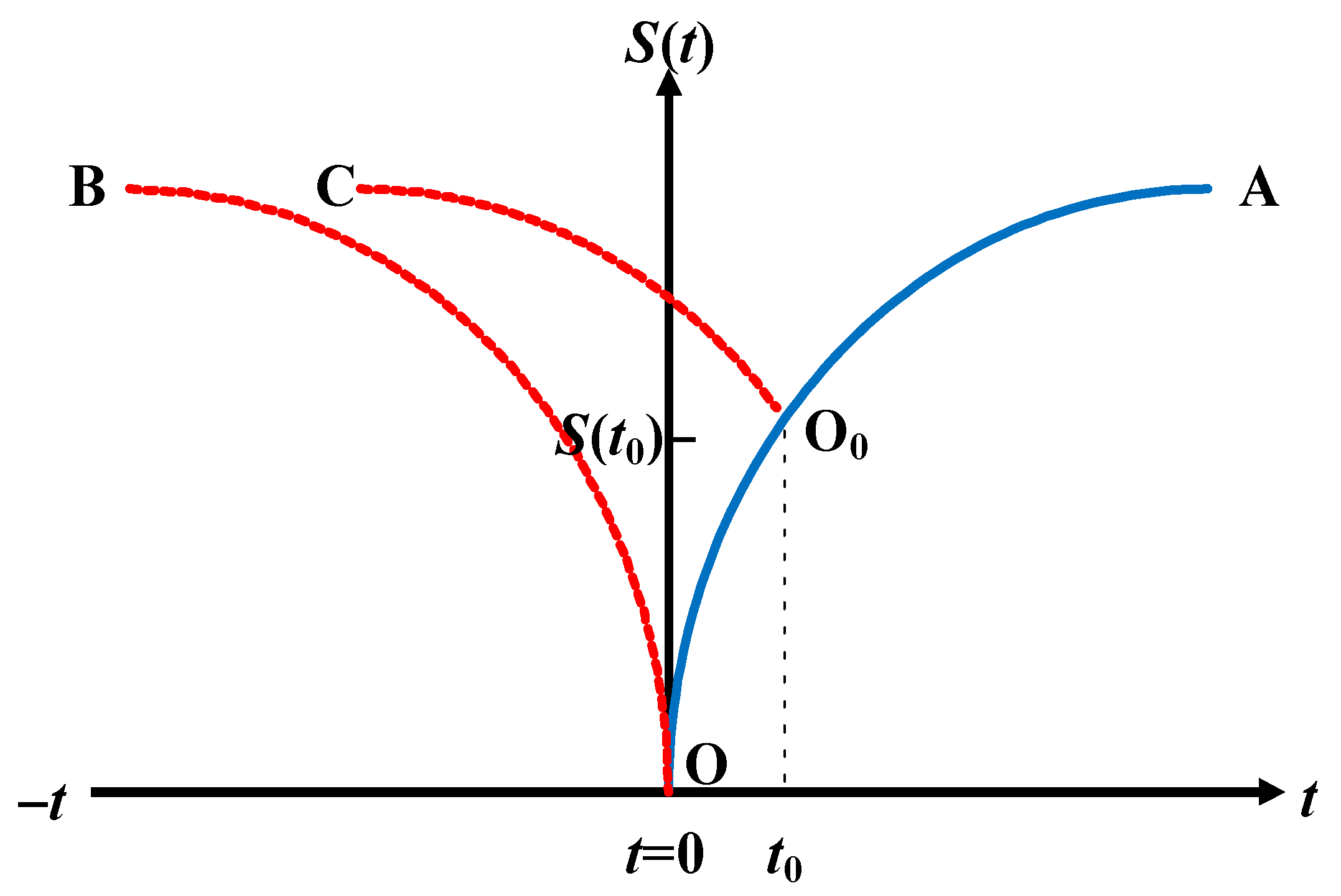
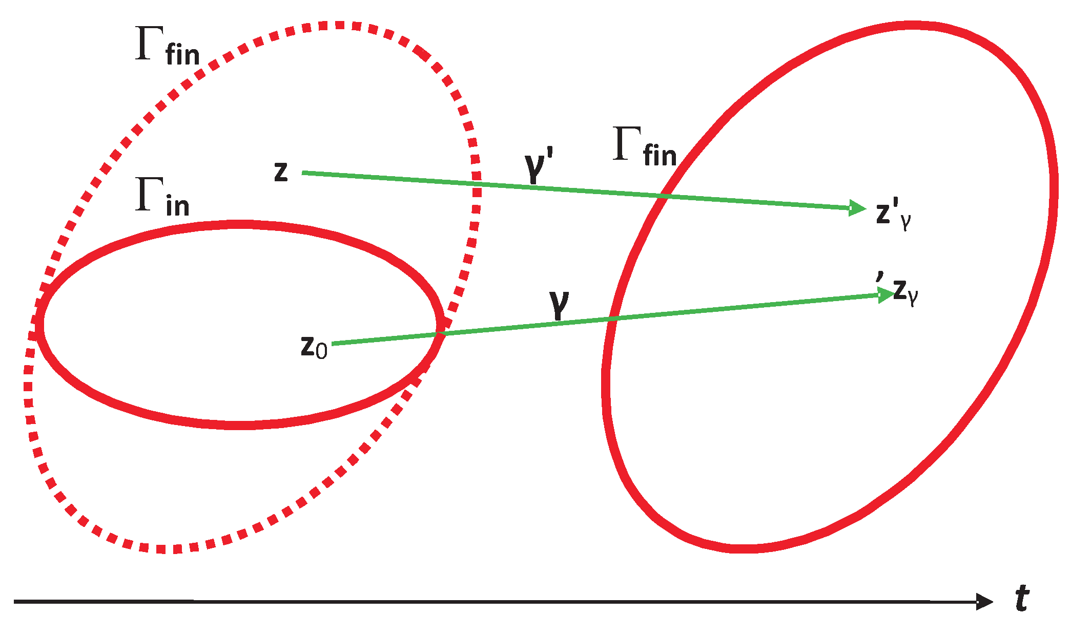