1. Introduction
The wave nature of material particles, conceived by de Broglie in 1923 [
1], still appears strongly counterintuitive today although confirmed by all the experiments carried out to verify it. There are at least two aspects of the particle–wave duality that seem contrary to common sense. The first is the “delocalization” of the corpuscle, i.e., the fact that an individual entity is somehow simultaneously present on the entire spatial volume occupied by the wave [
2]. Secondly, if we accept, as we do in this study, the standard formulation of quantum mechanics and, therefore, the projection postulate [
3], then in a “quantum jump” originating from the interaction with other particles or fields, the corpuscle abruptly changes its state of delocalization. As a particular ideal limit case, the corpuscle can undergo a precise localization in space acquiring, at least in an ephemeral way, an attribute of position. That same attribute is permanently possessed by a “classical” corpuscle.
The difficulties, however, do not end here. Amplitude interference experiments with single particles clearly demonstrate [
4,
5,
6] the absence of the trajectories attributable to quantum “corpuscles”. These experiments have become, at least since the 1960s, the basis of a didactic presentation of the particle–wave duality [
7]. A widely used example is that of Young’s interferometer with a double slit. In this device, the particle, which manifests itself as a localized corpuscle in its impact on the rear screen, interferes with itself as a consequence of the fact that the absence of trajectories prevents the definition of which slit is actually crossed.
A similar phenomenon occurs with two identical particles emitted in a coherent way, which can hit two distinct detectors (intensity interference). In this case, there may be a situation (H
1) in which the particle emitted by source S
1 hits detector D
1, and the particle emitted by source S
2 hits detector D
2, or there may be another situation (H
2) in which the particle emitted by source S
1 hits detector D
2, and the particle emitted by source S
2 hits detector D
1. The absence of trajectories leads to the undecidability between H
1 and H
2, and therefore to an interference connected with this undecidability [
8,
9]. This interference is a particular effect of a general phenomenon correlated with the non-factorizability of the wave function of the system consisting of the two particles. This phenomenon is the entanglement [
10], and it constitutes a further aspect of the quantum domain that does not seem to admit a classical representation.
We are thus faced with the problem of how to find a viewable representation of the quantum phenomena that we have briefly mentioned. In our opinion, this problem has a well-known historical precedent in the development of non-Euclidean geometries, in particular the elliptical geometry of Riemann [
11] and the hyperbolic geometry of Bólyai and Lobačevskij [
12,
13]. In an attempt to construct a geometry that denies the parallel postulate, we are faced with spaces that are impossible to visualize. Certainly, no one is able to visualize a space where, given a straight line and a point external to it, no parallel to the given straight line passes through that point. Or, an infinite number of parallels pass through it. This impossibility, however, persists only as long as we keep the original Euclidean notions of “ straight line” and “point”. It is, in fact, well-known that Riemann’s elliptical (two-dimensional) geometry admits a representation on the surface of a Euclidean sphere when the appropriate redefinitions of the terms are performed, for example, if the straight lines are interpreted as the maximum circles of the Euclidean narrative [
14]. In the same way, it is possible to represent the hyperbolic (plane) geometry on a portion of the Euclidean plane through the construction of Klein [
14]. In the simplest version of this construction, the space is the internal region of a circumference (understood in the Euclidean sense); the “straight lines” are (in Euclidean terms) the segments inside the circumference that intersect it in two points, etc. In summary, it is possible to represent the unrepresentable by attributing a new meaning to the terms. By carrying out this operation with care, the “new” can be represented, in a fully viewable way, in the same environment as the “old”. It should be emphasized that this operation is analogical, and numerous alternative representations of the same represented structure are possible.
Returning to our specific problem, the application of this type of strategy, first of all, involves the identification of a specific classical setting within which to operate the redefinition of the terms “particle”, “wave”, and “quantum jump”. It is then necessary to show that the entities thus redefined (but easily visualized in the chosen classical setting) behave like the corresponding quantum entities in the context of their relations. The intuitive comprehensibility of the redefined entities is guaranteed by their coexisting “narration” in classical terms.
In attempting to search for a representation of quantum phenomena intended in this way, it seems inevitable to start with the concept of “particle”. It is immediately evident that the usual notion of localized entity is unsuitable because it conflicts with delocalization and the absence of trajectories; therefore, something geometrically less constrained is needed. We choose to assimilate the particle to an electromechanical actuator (a sort of relay) that exchanges the energy elements associated with a charge. Recall that a particle can carry different types of charge: certainly, a gravitational charge but also possibly a weak, strong, or electric charge. We will deal with the concept of the charge assimilating it to that of electric charge, in both cases, keeping in mind the more general meaning of the term.
The next problem is how to introduce a spatially delocalized charge. The first idea that arises to mind is that, in each point of the empty space, there is a “charge reservoir” (i.e., a system of capacitors) that exchanges the elements of energy with the actuator, i.e., with the particle. The charge and energy of the particle are thus spatially delocalized because they are derived from the contribution of the capacitors associated with each point in space. The wave function of the particle then measures the local contribution to the total charge of the particle.
Invading the empty space with circuits of electric capacitors may appear as an annoying reminiscence of 19th-century English physics with its “ether of space”. It is, therefore, appropriate to repeat that the meaning of our proposal is not to specify what a quantum particle is but how it can be told using the language of classical physics. Our “ether of capacitors” is fictional but functional for that purpose. Its state of charge allows us to define the wave function of the particle.
Having in mind these reasons and this strategy, in
Section 2, we move on to examine the basic ideas of our representation and then introduce, in the subsequent
Section 3, the relevant definition of the wave function. An electrical analogy of the quantum jump is presented in
Section 4, which also discusses the reason why the wave function “lives” in the enlarged configurational space and not in ordinary spacetime. The notion of a multi-particle–wave function is thus introduced, and the meaning of entanglement is illustrated. In
Section 5, some issues related to the wave–particle dualism are specified; in particular, the notions of particle and corpuscle in the context of the present representation. The inclusion of the spin is discussed in
Section 6.
Section 7 summarizes the conclusions.
2. Basic Ideas
Let us now see how to express, in a more precise way, the ideas illustrated in
Section 1. For the moment, we limit ourselves to considering the case of the propagation of a single particle with mass
m, and only subsequently will we consider the more general case of a system with several particles.
We assume that the propagation of the particle in four-dimensional spacetime is associated with a phenomenon of the polarization of the vacuum, structured as follows: We denote a generic point of the four-dimensional spacetime by
x, whose coordinates in reference to the rest of the particle are (
x,
y,
z,
ct), and we consider the two regions of the light cone (past and future) having vertices in
x and extension ±
L/
c in
t. There are no stringent indications on the value of
L; we will assume that
L =
ħ/
mc is the Compton length of the particle. This assumption seems plausible because it is below this spatial scale that the particle is dissociated into particle–antiparticle pairs, and therefore, the polarization effects are manifested [
15]; however, any other physically reasonable choice of
L is just as good.
As a consequence of the vacuum polarization associated with the particle, two opposite charges of +
Q1(
x) and −
Q1(
x) will be induced in the future light cone of
x (
t <
t’ <
t +
L/
c), while two opposite charges of +
Q2(
x) and −
Q2(
x) will be induced in the past light cone of
x (
t −
L/
c <
t’ <
t). We pose
Q1,
Q2 ≥ 0 (the opposite choice is just as good). If we admit the existence of “vacuum capacity”
C, dependent only on the type of the particle (electron, muon, etc.), these two charges correspond to two energies
Qi2/2
Cn,
i = 1, 2. The total energy (
Q12 +
Q22)/2
Cn =
Q2/2
Cn is that of a group of
n(
x) capacitors in parallel to the same capacity
C brought to the common voltage
V. The voltage
V is assumed to be independent of
x. The charge
q =
CV then depends on the type of the particle. From the usual formalism of capacitors in parallel [
16], we have
Q2/2
Cn =
nCV2/2, from which the relation
Q =
nq follows.
A group of capacitors in parallel is, therefore, associated with each point-event x. The key assumption is that this group contributes, with a part of its charge Q, to the total charge of an actuator (the particle), which we will assume to be q.
If the particle was exactly localized in x, its charge would be integrally supplied by the capacitor group present in x. In this case, the total energy of the group would vary by an amount of ±q2/2Cn. The negative sign corresponds to the transfer, by the group, of charge q to the particle; the positive sign corresponds to the transfer, by the particle, of charge q to the group. In the hypothesis of the perfect localization of the particle in x, the number of possible energy elements that can be exchanged between the group and the particle is given by the ratio (Q2/2Cn)/(q2/2Cn) = (Q/q)2 = n2.
This suggests how to deal with the more general case of a delocalized particle. The charge exchanged between the group and the particle is, in this case, a fraction (possibly infinitesimal) of
q. We can, therefore, assume
ρ(
x)
dxdydz =
dn2(
x)/
A as the probability of the presence of the particle in the neighborhood
dxdydz of
x. The dimensionless normalization constant
A can be determined according to the relation:
The contribution to
q2 of the element
dxdydz around
x is then
q2ρ(
x)
dxdydz =
q2dn2/
A =
dQ2. Each point of space contributes, with its own group of capacitors in parallel, to the total charge
q of the particle. This result constitutes a description of the delocalization of the particle in classical terms, and we will return to it later. At the Compton scale (the minimum scale at which the wave function is defined [
15]), the relation
q2ρ =
dQ2/(
dxdydz) becomes
q2ρ~
Q2/
L3. Since
q does not depend on
x, the density (
ρ) is locally proportional to
Q2.
We must now see how the other actor appears, namely the wave function of the particle.
3. Positional and Impulse Representation
Let us now consider the two complex conjugate functions:
As we have seen, the probability density ρ is proportional to Q2 = Q12 + Q22 since q is independent of x. Therefore, ρ is proportional to ψψ*. We interpret functions (2) and (3) as the two wave functions, retarded and advanced, of the particle. We note that:
- (1)
If charges Q1,2 are multiplied by a real common factor (k), the probability density (not normalized) is multiplied by k2, while (2) and (3) are multiplied by k;
- (2)
If k is complex, the (non-normalized) probability density is multiplied by kk* when (2) and (3) are multiplied by k and k*, respectively. This implies that the modulus of (2) and (3) is multiplied by the modulus of k, while the two functions are rotated around the origin of the complex plane by an angle equal to the argument of k, k*;
- (3)
From both the proportionality of (2) and (3) to the capacitor charges and the additive nature of the charges, it follows that functions of this type can be summed generating interference effects;
- (4)
The time inversion t→ −t implies the exchange Q1↔Q2, and then ψ↔ψ*;
- (5)
Functions (2) and (3) have, of course with reference to the representation discussed here, a clear ontic meaning as charge states of the network of groups of capacitors associated with the particle.
On the other hand, it is possible to derive (2) and (3) with respect to the spacetime coordinates. Dimensionally, the quantities
I1,2 =
c∂μQ1,2, where
c is the maximal speed, and
μ = 0,1,2,3 is the spacetime coordinate index, are currents. In functions (2) and (3), those that are the eigenfunctions of
c∂μ are also the eigenfunctions of the four momentums (
iħ∂0, -
iħ∂i),
i = 1,2,3. These eigenfunctions can be superposed, thus generating generic wave packets. It, therefore, becomes possible to replace (2) and (3) with analogous complex functions containing currents instead of charges, thus passing to the momentum representation:
In general, (4) and (5) can be modeled as a system of
n inductors in parallel, with individual inductance
M, through which the current
I = (
I12 +
I22)
1/2 flows. The energy of the single inductor is
Mi2/2, with
i =
I/
n as the current flowing in it. The total inductance of the system is
MT =
M/
n. We, therefore, have [
16]:
The representation in terms of inductances is completely specular to that in terms of capacitors, and in this paper, we choose to focus on the latter.
4. Multi-Particle Systems
The independent variable
x of functions
Q1(
x) and
Q2(
x) labels a group of capacitors connected in parallel. Therefore, there is a continuous quadruple infinity of these groups. In a quantum jump, functions (2) and (3) are zeroed, and new
ϕ functions of the same type are generated at the output. This means that the capacitors associated with the labels
x = (
x,
y,
z,
ct), with
t = instant of the jump, are discharged and new capacitors associated with new labels of the same type are charged according to the functions
ϕ. It is possible to represent the quantum jump
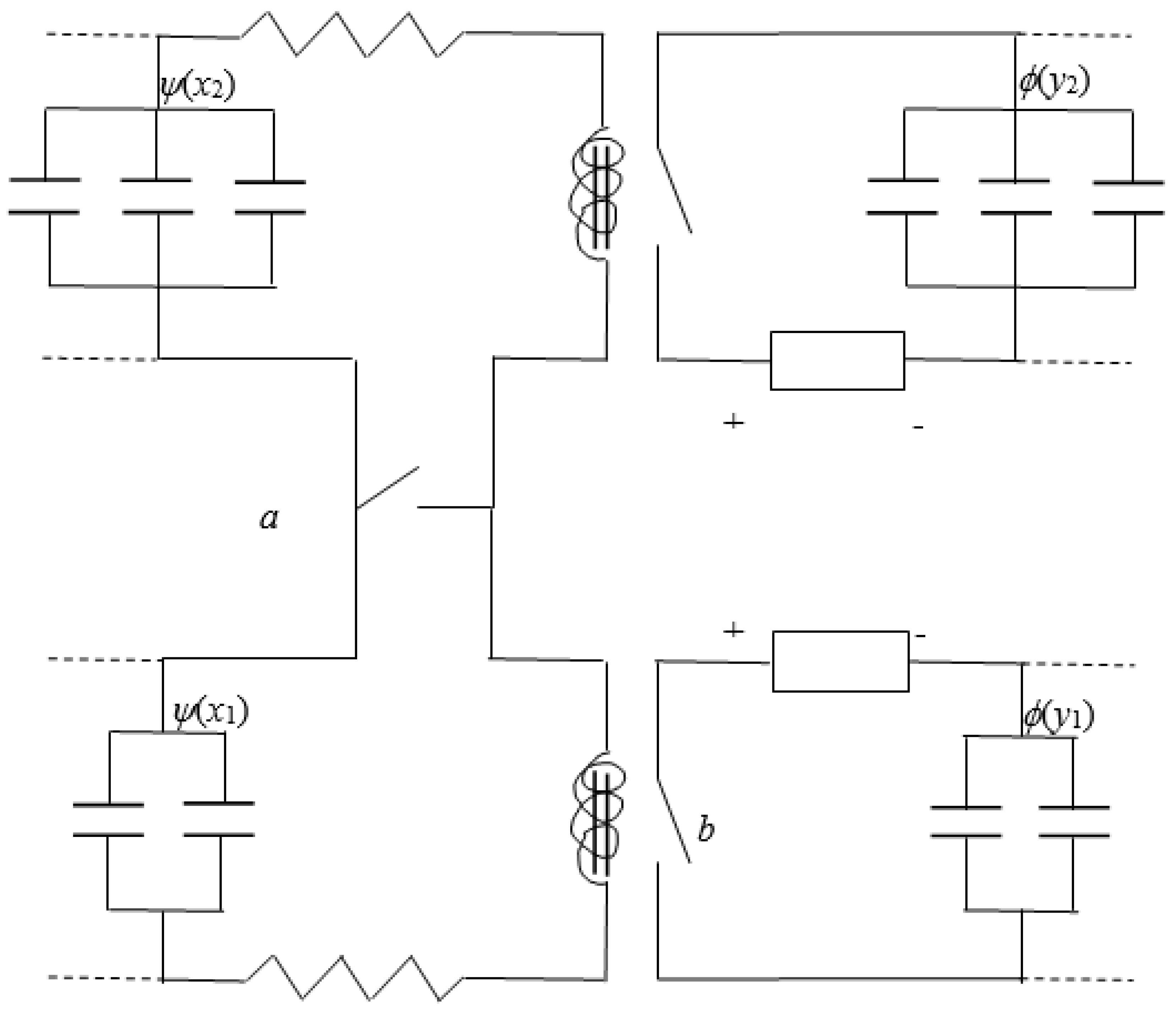
ψ→
ϕ with the electrical diagram in
Figure 1.
Each point-event of spacetime corresponds to a group of capacitors associated with the incoming function
ψ and a group of capacitors associated with the outgoing wave function
ϕ. There are, therefore, groups
ψ(
xi) paired with groups
ϕ(
yi), as in
Figure 1, where the labels
xi,
yi (
i = 1, 2, …) represent the same point-event, i.e., the same spatial position and same instant in time coinciding with those of the jump.
The homologous ends of all groups ψ(xi) are connected to the corresponding two ends of switch a. Closing a involves short-circuiting all the groups of capacitors associated with function ψ. The opposite charges are recombined, and ψ is canceled. The closing of a also implies, as an automatic consequence, the closing of other switches such as b. The latter, in turn, implies the charging of all the groups of capacitors associated with function ϕ.
The function of the electromechanical actuator constituting the particle is to keep the circuit associated with function ψ open, that is, to keep switch a open. The energy accumulated in the actuator is, therefore, the potential energy with switch a open. The interaction responsible for the quantum jump provides the energy needed to overcome this potential barrier and close a. At the end of the jump, a is closed, and its potential energy is zero.
It can be seen from the diagram in
Figure 1 that each value of the
x (
y) argument represents a mesh and, therefore, a discharge (charge) line. These labels are unique to the network of groups of capacitors that are discharged or charged. If the network corresponds to a particle, in the sense that it exchanges charge with that particle (actuator) only, then the label is shared by that particle. Two distinct particles, A and B, then have distinct spacetime labels of
xA and
xB. The wave functions associated with them are, respectively,
ϕ(
xA) and
φ(
xB), and each describes the state of the charge of the network associated with the corresponding particle. The overall state of the charge of the two quadruple infinity of the groups of capacitors associated with the two particles will be represented by the product
ϕ(
xA)
φ(
xB). Normally, in this product, the two functions are considered at the same instant in time, in such a way that the square modulus of the wave function provides the compound probability density of the two particles at that instant.
On the other hand, it is possible to imagine multiple networks and an equal number of actuators that (1) exchange charge with each network and (2) contribute to the potential energy related to the opening of the circuit of each network. In this case, the spatial labels of all the networks must be simultaneously assigned to the single actuator (particle). An example can be made by returning to the previous case of the two networks of A and B. Imagine two actuators (particles) to whose charge both networks contribute and each of which contributes to the opening of both circuits A and B. In this case, it is not possible to distinguish the two particles through their network, and one can have an entangled state such as, for example, ϕ(xA)φ(xB) ± ϕ(xB)φ(xA). This entanglement describes the contributions of the two networks to the opening of the two switches a, inserted, respectively, on network A and network B.
The proposed representation, therefore, allows us to define both single-particle–wave functions and multi-particle–wave functions, the latter both factorizable and entangled. It also supports a viewable model of quantum jump.
5. Corpuscle–Wave Dualism
It is possible to assume that the energy of the actuator constituting the particle associated with the wave function
ψ is
q2/2
C, with the meaning of the symbols already seen in the previous sections. In this hypothesis, this is the minimum energy required to keep switch
a open and thus allow the propagation of
ψ. It is, therefore, natural to suppose that, for a particle with mass
m, the rest energy of the particle is
q2/2
C =
mc2. This is, in fact, the minimum energy required for an interaction to create an outgoing state containing that particle. The delocalization of the particle described in
Section 2 and
Section 3then corresponds, physically, to the delocalization of its rest energy; the energy stored in each capacitor group represents the local contribution to the rest energy. The relation
q2/2
C =
mc2 in turn implies
C = 2
πε0rcl, where
ε0and
rcl are, respectively, the dielectric constant of the vacuum and the classical radius of the particle;
rcl/
L is the fine structure constant.
In summary, the quantum wave is the state of the charge of capacitor networks. Each network contributes to the charge and energy of an actuator, which is the particle. In this sense, the particle is “delocalized” on the network. The wave function defines, at the same time, the state of the charge of the network and the delocalization of the particle. Different particles can correspond to different networks, and in this case, the state of the charge of the networks is described by a factorizable wave function. On the other hand, when different networks contribute to powering the same actuator, and the latter acts on all the networks that feed it, entanglement occurs. In both cases, the wave function depends on the spatial coordinates of all the particles involved and not on the generic spacetime coordinates (as it would be for a classical field). The ambient space of the wave function is, therefore, the enlarged space of configurations, not the ordinary four-dimensional space where an observer coordinates the interaction events.
In a quantum jump, there is a sudden change in the wave function: The wave function entering the jump is zeroed by short-circuiting the network of capacitors associated with it; a new capacitor network, associated with a new wave function coming out of the jump, is charged. The net charge q of the particle—if it is a conserved quantity—is transferred from the incoming function to the outgoing one and becomes an additive contribution to the total charge of the particles it describes. This transfer is what we normally refer to with the term “corpuscle”. This definition captures a feature of the corpuscular aspect of the matter that is well-known from quantum experiments: its ephemeral nature. In other words, a corpuscle is an event (such as, for example, the impact of an electron on a photographic plate), not a persistent object that can be recognized and traced within the wave function.
The analogical representation proposed here applies to the wave function of systems with one or more particles. It is not applicable to the wave function of idealized systems such as the rotator, the vibrator, etc., because, for these systems, the concept of a charge associated with a (virtual) polarization of the vacuum loses meaning. It must, however, be considered that the real systems corresponding to these idealizations can nevertheless be described as the aggregates of interacting particles, and therefore, their exact treatment leads back to the case examined here.
At this point, we would like to introduce a clarification to avoid misunderstandings. It could be assumed that the vacuum polarization postulated in this paper coincides with the vacuum polarization described by quantum field theory (QFT). This belief can be strengthened by our choice of the value of L as the Compton wavelength of the particle since this is precisely the scale below which the polarization of the QFT vacuum occurs. In reality, there is no obvious identification of the two phenomena.
We have introduced vacuum polarization as an ad hoc postulate, functional to a translation, in classical terms, of the quantum delocalization of the particle, that is, of its wave function. For relativistic reasons (i.e., the polarization of the QFT vacuum and, therefore, the dissociation of the particle into virtual particle–antiparticle pairs, which occurs on the Compton scale), the concept of wave function loses its meaning on the Compton scale [
15]. Therefore, the Compton scale is the minimum scale at which the vacuum polarization,
as introduced in this paper,can be matched to the wave function of a massive particle. For this reason, we choose the value of
L as corresponding to the Compton wavelength of the particle.
Our classical description of particle delocalization starts from the vacuum polarization as postulated by us, through the introduction of an entirely fictitious “ether of capacitors”, invented only for this purpose. These capacitors exchange, with an actuator, fractions of the renormalized charge of the particle.
The polarization of the QFT vacuum around a bare charge leads, in the QFT, to the virtual charges of opposite signs, each of infinite value. In the QFT description, these charges renormalize the bare charge (also infinite), producing a finite effective charge at finite distances. These virtual charges have no obvious relationship with the fractions of the renormalized charge considered here, exchanged between the capacitors and the actuator. It is also not clear what this exchange would correspond to in the QFT description. Therefore, although an indirect connection between the polarization of the QFT vacuum and the phenomenon of polarization postulated in this work cannot be absolutely excluded, we limit ourselves to assuming the latter as a simple classical analogy useful for our purposes.
We conclude this section with an observation of resistance
R in the series with the capacitor network (
Figure 1). We assume the quantum jump, and therefore the discharge of the capacitors, as instantaneous. Strictly speaking, this would require a null time constant
τ =
RC (due to the normalization condition,
C is substantially referred to as the single capacitor) and, therefore, a zero resistance
R and an infinite discharge current
i =
V/
R =
q/
RC. This hypothesis is sufficient for our purposes. If we wanted to contemplate the hypothesis of a finite duration of quantum jumps, the time constant of the discharge must be finite. In such a case, experimental data provide an upper limit of
τ, intended as “jump duration”; they then set an upper limit on the value of
R and a lower limit on the value of
i. The technology of the exploration of the motion of atomic electrons by means of pulsed laser beams had a prodigious development in recent decades, passing from the pulses of the duration of the femtosecond to the pulses of the duration of the attosecond (10
−18s) [
17]. On this time scale, it is possible to resolve the temporal evolution of atomic orbitals during a transition, but it is not yet possible to resolve the quantum jumps that terminate this transition. The duration of the jumps—if actually finite—must, therefore, be much shorter.
Referring to the electron, the most studied elementary particle, it, therefore, seems reasonable to assume τ ~ rcl/c = 0.937·10−23s, and then C = 2πε0rcl = 1.56·10−25F; R = τ/C = 60 Ω; i = e/τ = 17,100 A. These results are derived from the currently accepted value for the classical electron radius, rcl = 2.81·10−15m. However, we do not elaborate here on this aspect, due to its speculative character.
6. Spin
It is possible to construct the row or column vectors whose components are different functions of types (2) and (3), or, respectively, of types (4) and (5). Each component of these vectors is associated with a different network of groups of capacitors in parallel or, respectively, of inductances in parallel, afferent to a single actuator. If the relativistic covariance rules are applied to these vectors, they become spinors. We then have the Pauli spinors in the non-relativistic limit and the Dirac spinors in the general relativistic case. It thus becomes possible, in principle, to extend the present electrical analogy to include the spin of elementary particles and their internal degrees of freedom such as isospin or strangeness. Here, we limit ourselves to an observation on the spin.
A generic wave function of spin ½ takes, in the Pauli algebra, the following form [
18,
19]:
where
is the spatial position, and the spinors
and
represent fully polarized beams along the
z axis, corresponding to the two eigenvalues of the spin projection along that axis. The meaning of (7) in the present representation is that a single actuator (particle) exchanges charge with two distinct networks, each of which is associated with one of the two projections, and keeps them both open. The (complex) coefficients
α and
β measure the relative intensity of the exchange with the relevant network, in the terms seen in
Section 3. The rotation of the frame of reference of an angle
χ around a spatial axis
(with
= 1) changes coefficients
α and
β according to the following law [
18,
20]:
For example, if
and
, a rotation around the
z axis gives
,
. This means that the exchange is sensible to rotations. It must be borne in mind that a variation in axes is always associated with a modification of the experimental situation, such as fixing a direction to a magnetic field or reorienting a polarizer. This modification involves a variation in the charge exchange between the particle and the two networks. The directional dependence of the exchange represents, in a certain sense, a directional structure of the particle itself. However, this structure, or the internal “direction” of the particle, has nothing to do with the rotation of a solid object in three-dimensional space. This is consistent with the non-classical nature of the spin [
21].
7. Conclusions
In these concluding notes, we would like to try to put this contribution in context. In our opinion, the non-viewability of quantum processes has generated the widespread belief that they are inherently incomprehensible. Quantum theories are often assimilated into formal recipes that are very effective on the predictive level but are ones whose connection with any intelligible ontology remains obscure. Following the historical precedent of non-Euclidean geometries, we tried to circumvent these obscurities by providing a model of quantum behavior in a classical context: that of electrical circuits. As in the case of non-Euclidean geometries, we had to redefine the notions of particle, wave, and corpuscle in this context, moving away from their original classical meaning. By paying this price, we obtained the visualization of quantum entities and processes, guaranteed by the classical nature of the context in which their redefinition was carried out.
We believe that this attempt is located in a sort of middle land between the choice of surrendering to non-visualization (with the consequent problems of conceptual opacity) and the strong choice of determining an ontology of elementary processes, which is the goal of any physical interpretation of the quantum formalism. Although in choosing our representative model, we tried to adhere to the criteria of “sound physics”, we find it difficult to seriously believe that space is the equivalent of a cabinet of electric capacitors. Our representation is, therefore, less than a sensu strictu interpretation of quantum formalism such as, for example, Bohm’s [
22] and relative state [
23] interpretations. At the same time, however, it is more than just a surrender to mystery and allows for an analogical narrative of concepts such as the wave function or the particle–wave dualism. Our aim is to facilitate the communication related to quantum processes, through images that can be understood by anyone familiar with the basics of classical physics concerning electrical circuits.
This objective responds to a pedagogical need that has been our strongest motivation and seems particularly urgent to us in a moment like the present one, in which quantum theories have become part of the educational background of the new generations of engineers and technologists, engaged in the development of the amazing technologies that the quantum nature of reality makes possible.


