Comparative Performance of NIR-Hyperspectral Imaging Systems

Abstract

Near-infrared spectroscopy (NIRS) allows for the rapid estimation of a wide range of wood properties. Typically, NIRS studies on wood have utilized benchtop spectrometers, but efforts to utilize NIR hyperspectral imaging to examine wood and wood products have increased. Compared to benchtop NIR systems, hyperspectral imaging has several advantages (speed, visualization of spatial variability), but the data typically have a lower signal-to-noise ratio as well as fewer wavelengths saved; thus, hyperspectral imaging systems have a larger spectral sampling interval (SSI). Furthermore, the SSI and wavelength range varies considerably among different HSI cameras. NIR-HSI systems based on indium gallium arsenide (InGaAs) detectors have a wavelength range typically from 900 to 1700 nm, while short-wave infrared hyperspectral imaging (SWIR-HSI) systems based on mercury cadmium telluride (MCT) detectors have the ‘full’ NIR wavelength range from 1000 to 2500 nm. These factors may influence the performance of wood property calibrations. We compared one NIR-HSI (900–1700 nm) and three SWIR-HSI (1000–2500 nm) commercially available cameras with an NIRS benchtop spectrometer (1100–2500 nm). The performance of specific gravity (SG) and stiffness (MOE) calibration models was compared with one-hundred Douglas-fir (Pseudotsuga menziesii) samples. The limited wavelength range of an NIR-HSI camera provided the best models for MOE, whereas the NIR-HSI and two SWIR-HSI cameras provided similar SG results. SWIR-HSI models heavily favored wavelengths greater than 1900 nm.

1. Introduction

Near-infrared spectroscopy (NIRS) provides a rapid option for the estimation of a wide range of wood properties [1] and is now frequently employed, either alone or in conjunction with other techniques, for nondestructive evaluation. Typically, NIRS studies have been based on spectra collected using benchtop spectrometers where the sample (solid wood, milled wood, or in some examples, chips) is placed in front of the near-infrared beam or the spectrometer is fitted with a fiber optic probe. Conventional NIRS provides very high spectral intervals, but the spectral information is limited to a relatively small spatial area. This may be disadvantageous if the materials being analyzed, such as large wood specimens including logs, lumber or even cross-sectional discs, are heterogeneous spatially and spectrally, making it difficult for a spectrometer to adequately represent within-sample variations without collecting spectra from multiple sampling locations.

Options for increasing the area examined without collecting multiple spectra from solid wood involve using a spectrometer with a large spot size [2], moving short-clear samples [3] or even lumber passed the NIR beam [4,5], or for milled wood using a rotating sample holder. Hyperspectral imaging (HSI) provides a new and potentially more suitable option for analysis of heterogenic materials because it can scan larger areas more rapidly than single-point measuring NIRS. HSI combines spectroscopy and digital imaging and generates a hyperspectral image (a hypercube’) of 3D multivariate data, where pixels in a hypercube may contain different spectral responses associated with different chemical compositions and/or physical properties of materials of interest by measuring light absorbing and scattering [6].

NIR-HSI systems based on indium gallium arsenide (InGaAs) detectors have a wavelength range typically from 900 to 1700 nm, while short-wave infrared hyperspectral imaging (SWIR-HSI) systems based on mercury cadmium telluride (MCT) detectors have the ‘full’ NIR wavelength range from 1000 to 2500 nm, which is similar to benchtop NIRS spectrometers. The use of NIR-HSI and SWIR-HSI is rapidly expanding in a variety of related fields, ranging from plants and biological materials [7,8] to food quality and safety [9,10]. Similarly, wood-related NIR- and SWIR-HSI research has been increasingly reported in the literature, where cameras have been used to examine various spectral and spatial properties and variations of wood materials. Applications include the estimation of physical and mechanical properties of radial strips [11,12,13,14,15] and lumber [16,17,18] as well as the detection of compression wood [19,20], tension wood [21] and resin defects [22]. A common area of research has been the estimation of wood moisture content [23,24,25], and associated research includes an investigation of changes in the spatial distribution of water when wood is dried [20]. Recently, it has been used to examine wood–water interactions [26,27,28]. Studies have also examined chemical composition variation across the surface of discs [29,30] and across small sections (e.g., 4 mm² area) across radial, tangential and transverse surfaces [31]. Wood degradation either by fungi [32] or weathering processes [33,34,35] and treatments to protect wood, including acetylation [36,37], oil impregnation [38], thermal modification [39], and the concentration of phosphorus-based flame retardants [40], have all been investigated. Hyperspectral images have also been used for species classification [41,42], characterization of juvenile and mature wood [43], particleboard identification [44], and to investigate how the presence of knots and holes influences veneer modulus of elasticity [45]. On-line applications include the identification of wood chips with elevated extractive levels [46], the segregation of waste materials (including wood) [47,48,49] and monitoring the quality of extruded wood–plastic composites [50].

It has been demonstrated that the spectral data provided by NIR-HSI and SWIR-HSI could produce wood property calibrations whose performance was equivalent to those obtained using a benchtop NIR spectrometer [18,23]. These results are encouraging although, even with recent developments in HSI technology, hyperspectral cameras typically record fewer wavelengths (i.e., spectral sampling interval—SSI) compared to NIR benchtop spectrometers. Hyperspectral cameras also have a lower signal-to-noise ratio (SNR) because benchtop spectrometers average data from multiple sub-scans relatively quickly, while HSI for high-speed in-line scanning in industrial settings may not acquire multiple lines at the same spatial position to increase the SNR. Furthermore, hyperspectral cameras vary considerably in terms of their SSI and wavelength range, which may affect the performance of wood property calibrations measured with different cameras. Hence, the primary goals of this study were to (1) utilize and compare four different commercially available hyperspectral cameras (one NIR-HSI (900–1700 nm) and three SWIR-HSI (1000–2500 nm)) in terms of the calibration and prediction performance for properties (modulus of elasticity, MOE and specific gravity, SG) of based on HSI images of the transverse surface of one-hundred Douglas-fir (Pseudotsuga menziesii) samples and (2) compare the model performance of the hyperspectral cameras with a benchtop NIR spectrometer.

2. Materials and Methods

2.1. Specimen Preparation and Testing

Commercial mills in Canada, and Idaho, Oregon, and Washington, USA, each provided four packages of No. 2 grade, 2 × 4 (38 mm × 89 mm × 2438 mm) Douglas-fir kiln-dried lumber [51]. A total of 496 pieces of lumber (124 from each mill) were obtained from the mills. For each lumber sample, their dimensions, weights, and moisture contents were measured. The modulus of elasticity (MOE) and the specific gravity (SG) of each lumber were determined as described in [51].

Following the measurements described in [51], a radial arm saw was used to cut a block (38 mm × 89 mm × 51 mm longitudinally) from each piece of lumber for NIRS and HSI analysis. Only 390 blocks (Canada—88, Idaho—95, Oregon—109, Washington—98) were available (utilized in [18]). From the 390 blocks, a subsample of 100 was selected for this study with the aim of capturing the full range of values for MOE and SG and equally representing the different sampling locations.

2.2. Hyperspectral Imaging

Hyperspectral images were collected on four different instruments: three short-wave infrared (SWIR) HSI cameras identified as SWIR-HSI-I, II and III and one NIR-HSI camera. The scan time per sample was estimated to be 3–5 s for the different hyperspectral cameras utilized. For the benchtop NIR, the scan time was approximately 40 s per sample.

2.2.1. SWIR-HSI-I

The first set of hyperspectral images was collected in the wavelength range of 1000–2500 nm using a push broom short-wave infrared (SWIR) HSI system (Hyperspec^® SWIR, Headwall Photonics, Fitchburg, MA, USA).The system consisted of a spectrograph, a focal plane array with a Peltier-cooled 320 × 256 mercury cadmium telluride (MCT) detector (MCT-851 XC403, Xenics, Leuven, Belgium), a 30.7 mm front lens (OLES30, Specim, Oulu, Finland), two illumination sources with tungsten halogen lamps, a motorized linear slide (T-LSR300B, Zaber Technologies, Vancouver, BC, Canada), a computer, and in-house developed software (C++) for image acquisition and preprocessing, including intensity calibration and denoising. Two light sources oriented approximately 20° from the sample were used for illumination. For each image, a scan of an individual sample started, while a dark current reference was collected with the camera lens cap covering the lens. After acquiring about 10 lines of dark current signals, the lens cap was opened so that white reference signals were collected from a white diffuse-reflectance standard panel (Fluorilon-99W, Avian Technologies, Sunapee, NH, USA) with dimensions 25 mm × 300 mm, which was followed by scanning of the sample. The spectra were collected at approximately 8 nm intervals over the SWIR wavelength range. The background plate was stationary and black.

2.2.2. SWIR-HSI-II

The second set of hyperspectral images was collected in the wavelength range of 913–2519 nm (the average spectral interval of 6.2 nm) using a push broom SWIR-HSI system (Compovision, Sumitomo Electric Industries, Ltd., Tokyo, Japan). This SWIR-HSI camera was equipped with a spectroscope and a 2D photosensitive element with 256 (wavelength) × 320 (position) pixel dimensions. In this study, a wavelength range from 1002 to 2300 nm was selected for a higher SNR than using the full wavelength range. Line illumination was produced by two halogen lamps from two sides. The illumination angle was adjusted to 45°. Each sample was positioned on a slider and scanned line by line. The frame rate was set to 150 frames/s, and the exposure time was 6.0 ms. As a reference, a white plate (BaSO₄) was used under the same conditions, whereas dark images were obtained by completely covering the lens with its cap.

2.2.3. SWIR-HSI-III

The third set of hyperspectral images was collected using a push broom line scanning system Specim SWIR camera (Specim, Spectral Imaging Ltd., Oulu, Finland), covering the spectral range of 962–2544 nm with 288 wavelengths. The spatial resolution was 384 pixels corresponding to 130 mm of the field-of-view width (0.34 mm/pixel). The camera was installed on the LabScanner 100 × 50 (Specim, Spectral Imaging Ltd., Oulu, Finland). The sample placement table was coated with a black absorbing paint. A set of 14 tungsten halogen lamps illuminated a scanner table (width 500 mm) with an irradiation angle of 45°. The Lumo software supplied with the system was used for the image acquisition of samples as well as white and dark references. The black reference was acquired as 100 image scans with a closed shutter, while a white reference was acquired by slow motion (10 mm/s) scanning of the white Spectralon plate at the length of 80 mm (corresponding to 1600 reference images). The frame rate was 200 Hz with an exposure time of 2.40 ms.

2.2.4. NIR-HSI

The fourth set of hyperspectral images was collected in the wavelength range of 931–1718 nm (224 wavebands) using a push broom NIR hyperspectral camera (Specim FX17, Specim Spectral Imaging Ltd., Oulu, Finland) fitted with a focusing lens (Specim OLET 17.5 F/2.1). Tungsten halogen lamps illuminated a lumber sample, while the sample motion and image acquisition were controlled using application software (Specim Lumo) supplied with the system. For intensity calibration, a dark current and a white reference were collected before acquiring each hyperspectral image. The block samples were placed on a black background for quicker and easier object segmentation and data analysis.

2.3. Benchtop NIR (NIR-SPECT)

A FOSS NIR Systems Inc. Model 5000 scanning spectrometer (FOSS NIRSystems Inc., Laurel, MD, USA) was used to collect diffuse reflectance NIR spectra (1100–2500 nm, 2-nm intervals) from the cross-sectional (transverse) face of each block. To ensure a consistent area was scanned, a white Teflon mask (16.5 mm × 16.5 mm) was installed on the window where the NIR beam exits the spectrometer, and the lumber sample was positioned directly in front of the mask. From different locations on the transverse surface of each piece, two spectra were collected (each an average of 32 readings) and averaged, giving a single spectrum.

2.4. HSI Data Processing

Each image was calibrated with its own dark current and white reference signals using the equation:

$$\mathrm{R}=\frac{{\mathrm{R}}_0-\mathrm{D}}{\mathrm{W}-\mathrm{D}}$$

(1)

where R is the relative reflectance, R₀ is the measured reflectance, D is the dark current reference signal, and W is the white reference signal. The samples were isolated from the background by selecting a region of interest (ROI). Each sample’s ROI was decreased from the full sample size to eliminate possible edge effects. From within the selected ROI, spectral data were extracted and averaged to provide one mean spectra per sample per instrument. The relative reflectance values were transformed to absorbance (A), with the equation:

$$\mathrm{A}={\log }_{10}\left(\frac{1}{\mathrm{R}}\right)$$

(2)

Then, these absorbance values were used for subsequent data analysis.

2.5. Wood Property Calibration and Prediction of Wood Properties

Two sets of Partial Least Squares (PLS) regression calibration models were constructed in this study; the first used all of the available wavelengths provided by each instrument (

Table 1. Wavelength range, number of wavebands, full width at half maximum (FWHM) and spectral sampling interval (SSI) for each HSI camera and the benchtop spectrometer.

	Wavelength Range (nm)	# Wavebands	FWHM (nm)	SSI (nm)
SWIR-HSI-I	1000–2300	207	6.2	6.2
SWIR-HSI-II	1101–2503	185	8 to 10	7.4
SWIR-HSI-III	962–2545	228	12	5.6
NIR-SPECT	1100–2498	700	10	2
NIR-HSI	931–1718	224	8	3.5

#: Number of Wavebands.

), whereas the second was constructed using a wavelength range limited to 1100–1700 nm to be consistent with the largest wavelength of the NIR-HSI instrument and the smallest wavelength for the benchtop NIR-SPECT instrument. Standard normal variate (SNV) and second derivative (gap-segment method; gap = 0, segment = 5) spectral pre-treatments were first used to correct the baseline shifts mainly caused by light-scattering effects [52,53]. A subset of samples (75%) was randomly selected for the construction of MOE and SG calibration models. Leave-one-out cross-validation was used to obtain the calibration models. The predictive performance of the calibration models was assessed using the remaining samples (25%) as a test set. The calibration and test set samples were the same for each instrument, and the measured MOE and SG values had similar ranges between the calibration and test sets (

Table 2. Summary of stiffness (MOE) and specific gravity (SG) data for PLS regression analysis.

		MOE (GPa)				SG
	No.	Min	Max	Mean	SD	Min	Max	Mean	SD
Calibration	75	6.91	19.53	11.89	2.78	0.37	0.62	0.47	0.05
Prediction	25	8.44	18.61	12.58	2.57	0.37	0.60	0.48	0.06

No.: number of the data point, Min: minimum measured value, Max: maximum measured value, SD: standard deviation.

). The number of LVs was identified by analyzing model statistics where the optimal LV number was determined as a compromise between low model order, contribution rate and gain in the RMSE reduction. It was implemented by analysis of initial/first 15 LV determined for both calibration and validation data sets but limited to 6 for comparative purposes. The overall objective of this protocol was to minimize the risk of model overfitting and increase the overall reliability of prediction.

The performance of the constructed calibration model was characterized by the coefficients of determination ($R^2$) (Equation (3)) and root mean squared error (RMSE) (Equation (4)):

$$R^2=1-\frac{{{\displaystyle \sum }}_{i=1}^n{\left(y_i-{\hat{y}}_i\right)}^2}{{{\displaystyle \sum }}_{i=1}^n{\left(y_i-\overline{y}\right)}^2}$$

(3)

$$\mathrm{RMSE}=\sqrt{\frac{1}{n}{\displaystyle {\displaystyle \sum }_{i=1}^n}{\left({\hat{y}}_i-y_i\right)}^2}$$

(4)

where $n$ is the number of samples in the data set, $y$ is the MC reference values, $\hat{y}$ is their values predicted by the PLS regression analysis, and $\overline{y}$ is the mean values of $y$. Variable importance in projection (VIP) scores [54] were calculated to estimate the important wavelengths. A VIP score close to or greater than 1 can be considered important for model construction.

3. Results and Discussion

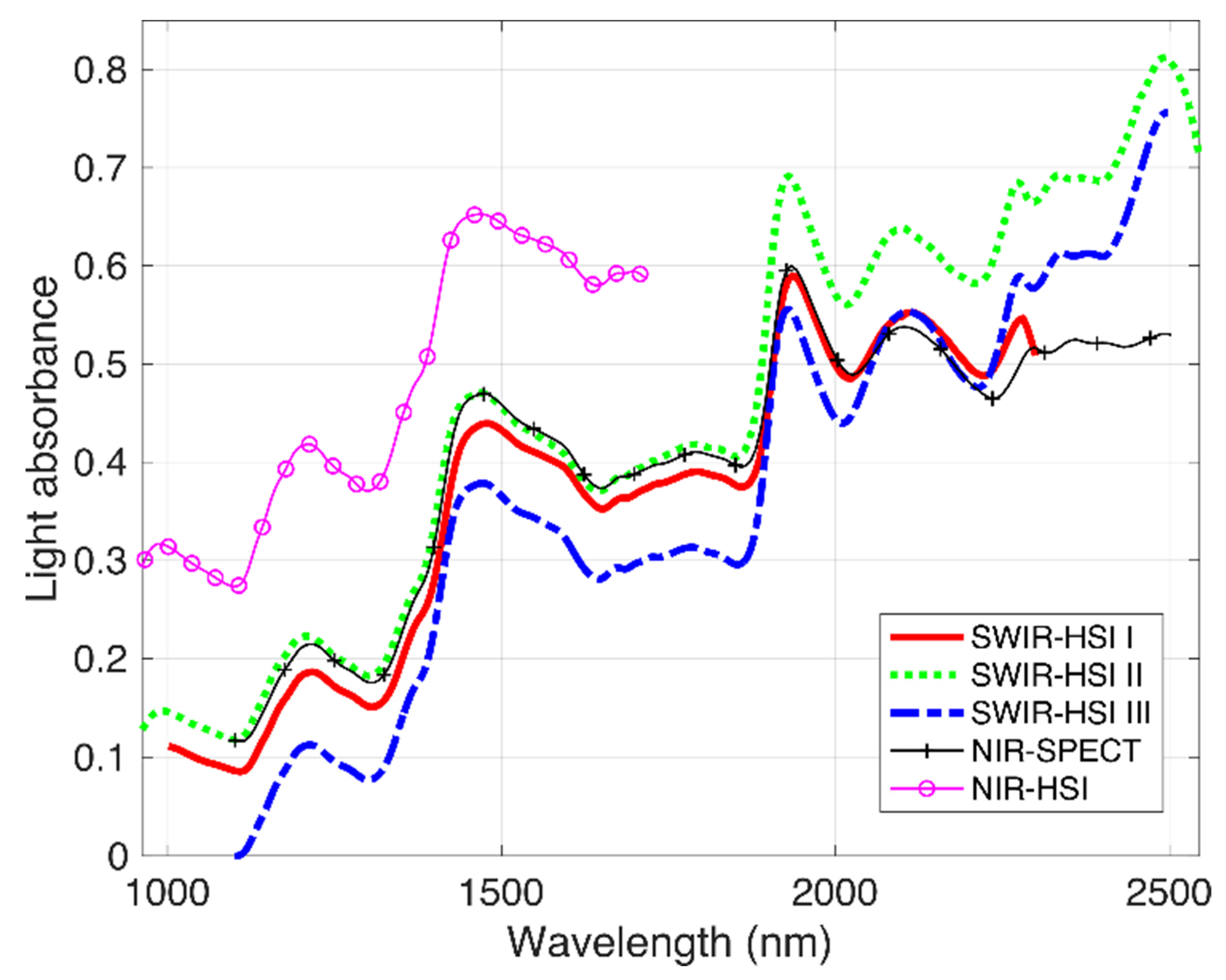
3.1. Comparison of Spectra

NIR spectra from the identified ROI on the transverse surface of the Douglas-fir samples examined by each NIR-HSI camera and NIR-SPECT are depicted in Figure 1. Compared to spectra obtained using NIR-SPECT (utilized here as a reference), spectra of the SWIR-HSI systems were all similar up to approximately 2000 nm, and then, differences in spectra amongst instruments become more apparent. In the spectral range of 2000–2500 nm, spectra based on images from the SWIR-HSI-I camera were most similar to the NIR-SPECT, which was followed by the SWIR-HSI-II camera, but absorbance values based on this camera decreased as wavelengths approached 2500 nm compared to the other instruments. SWIR-HSI-III in this region showed the greatest increase in absorbance beyond 2000 nm, but the spectra also appear nosier than other cameras in this region. NIR-HSI instrument spectra appear similar to those obtained using NIR-SPECT in the spectral range from 1100 to 1700 nm.

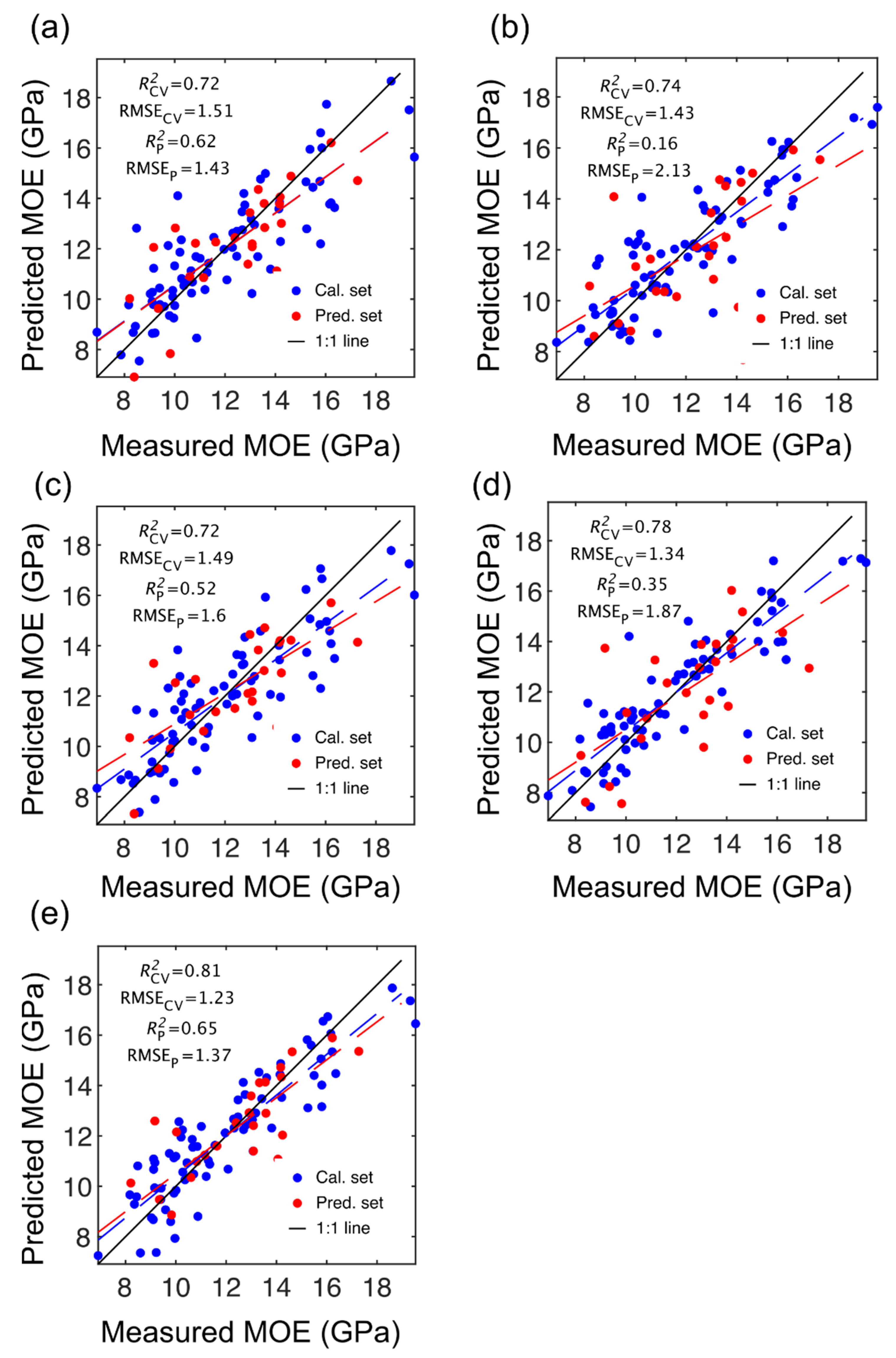
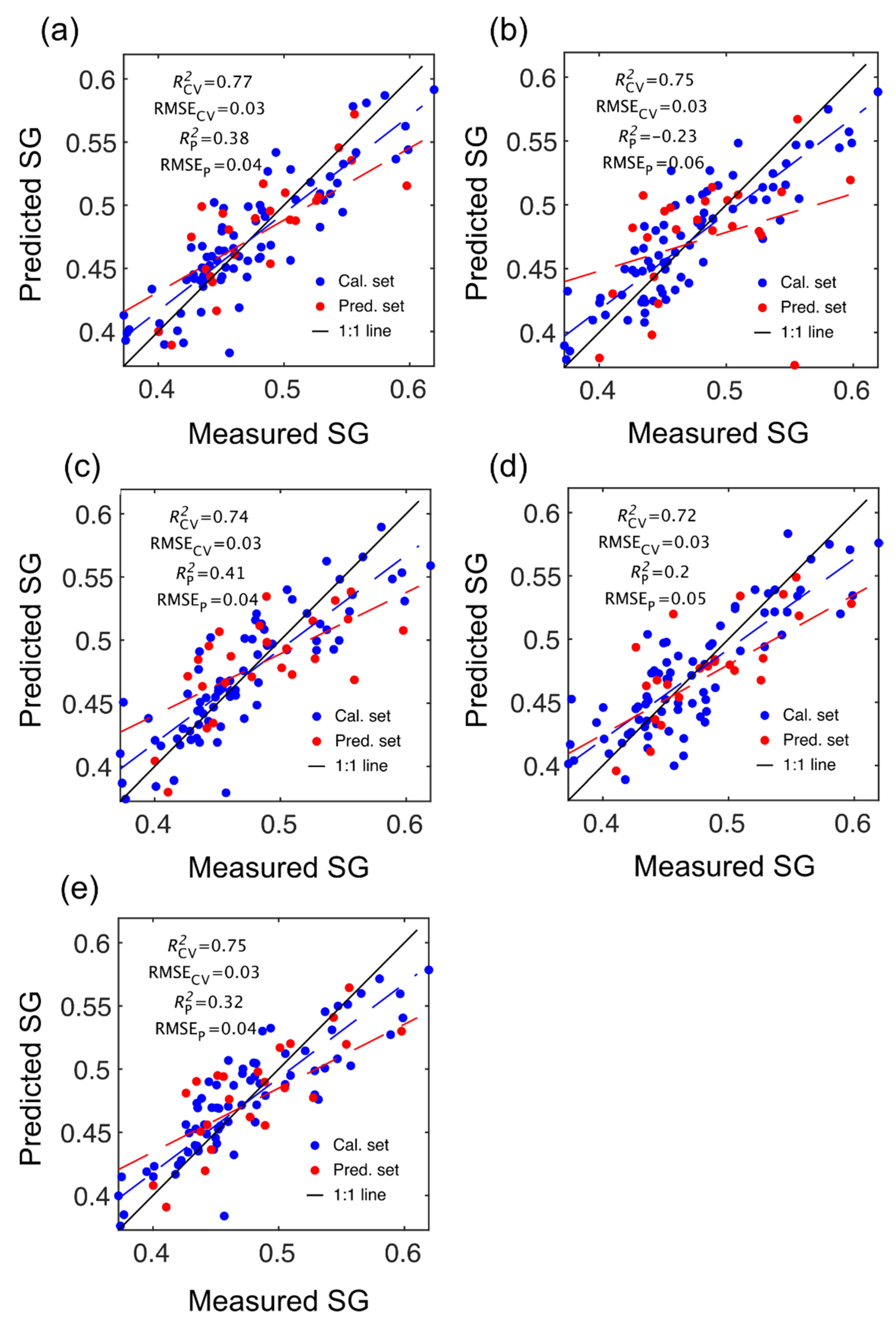
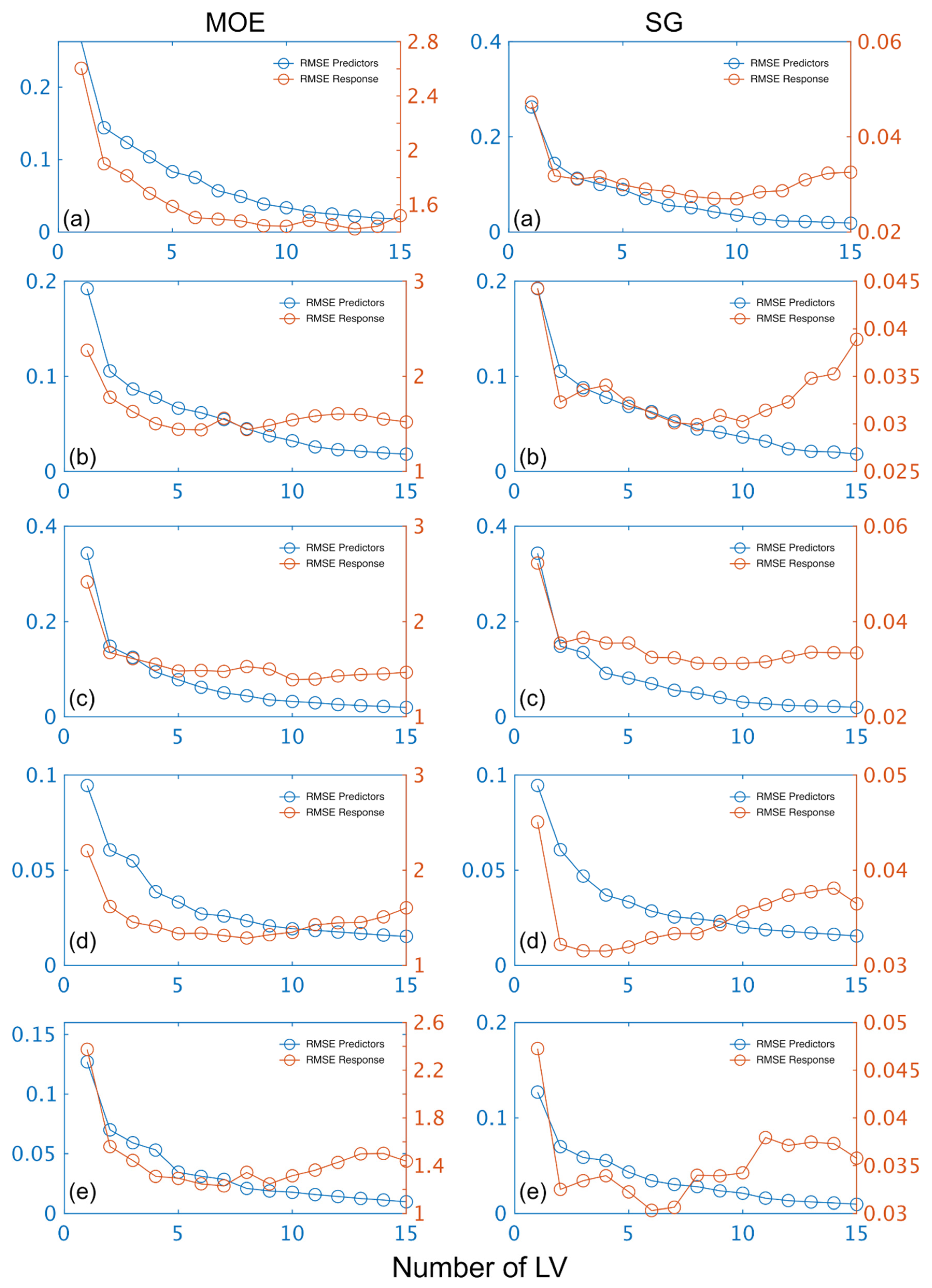
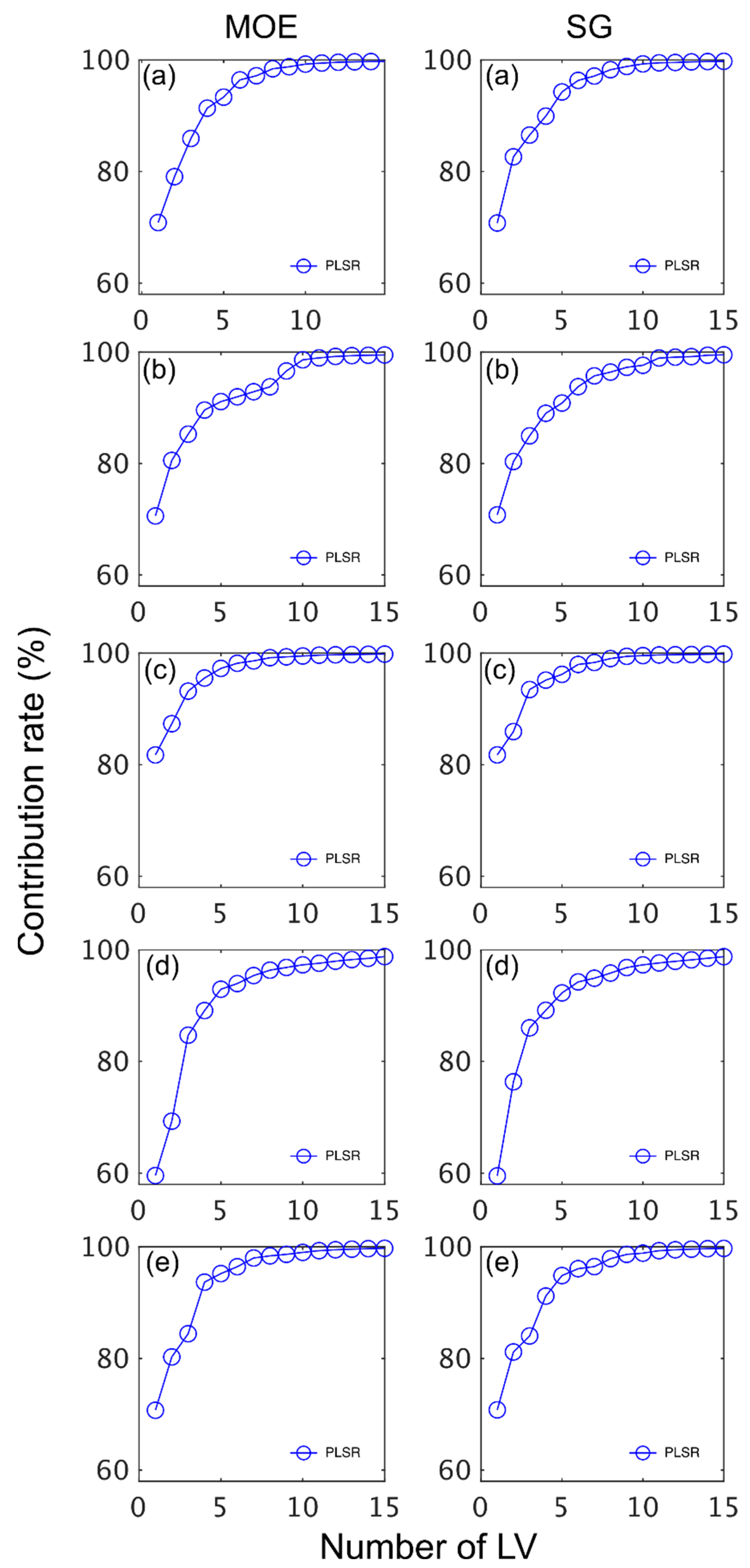
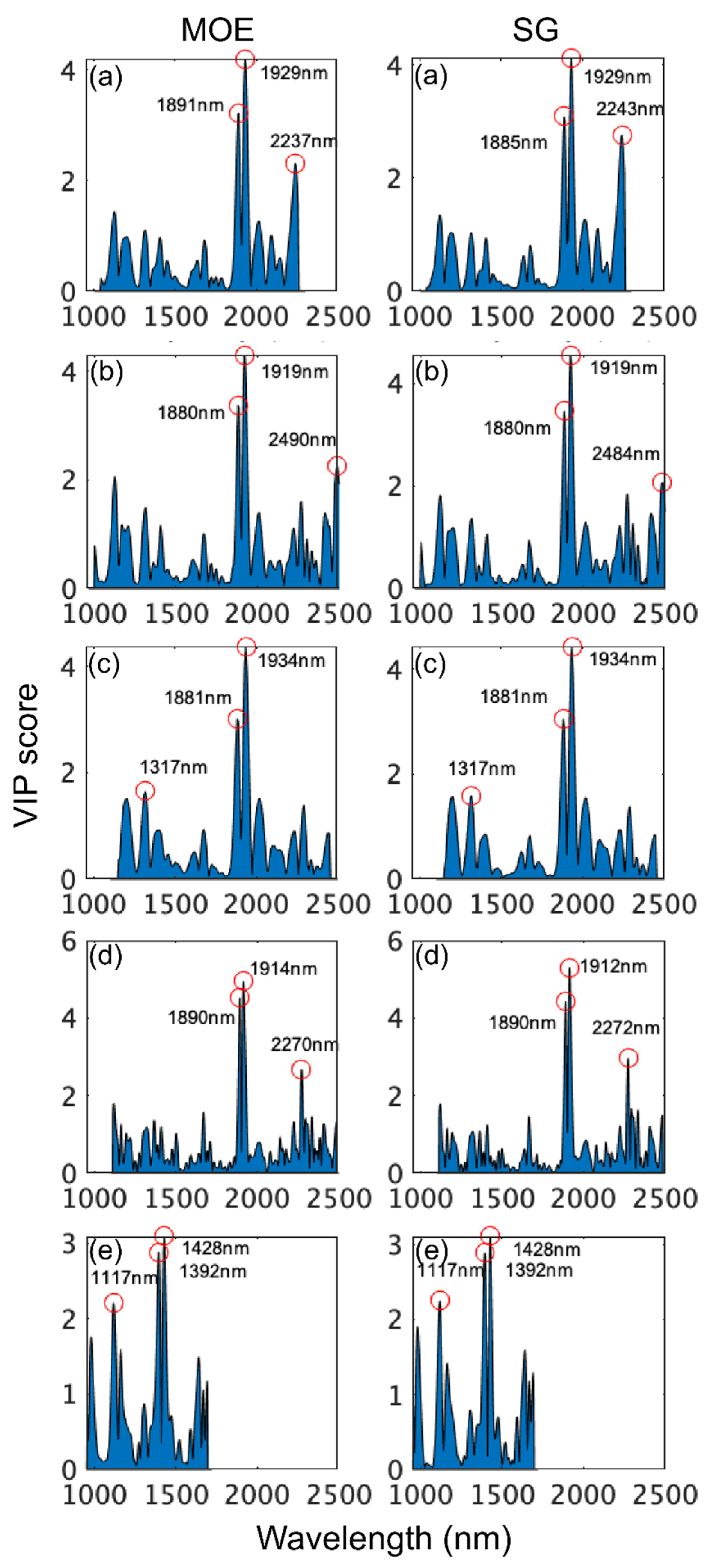
3.2. Calibration/Prediction—MOE and SG

Figure 2 and Figure 3 illustrate the calibration and prediction performance for MOE and SG models, respectively, which were obtained using the wavelength range provided in Table 1.

The number of LVs used was 6, and this number was selected for comparative purposes and based on plots of root mean square error (RMSE) plotted against number of latent variables (LVs) (Figure 4) and contribution of LVs to MOE and SG models (Figure 5). A notable result was the strong performance of the NIR-HSI camera compared to all other instruments, with its spectral data providing the strongest calibration/prediction of MOE when applied to the test set. For SG, the calibration statistics of the SWIR-HSI-I, SWIR-HSI-II and NIR-HSI cameras were similar; however, when applied to the test set, the SWIR-HSI-I camera provided the strongest predictions in terms of R²_test (RMSE_test values were similar). The models that provided weaker predictions had greater bias (deviation from the depicted 1:1 line). NIR-SPECT never achieved the best calibration/prediction accuracy, likely indicating that the spectra that were collected did not represent the transverse surface of the examined samples as well as those obtained by the HSI cameras.

The NIR-HSI performance, particularly for MOE, surpassed that of the full range instrument from the same manufacturer (SWIR-HSI-III). The SSI (5.6 nm vs. 3.5 nm) and FWHM (5.6 nm vs. 3.5 nm) are higher for the NIR-HSI camera and likely aided in achieving the observed results. The collection of spectral data was also different for the NIR-HSI camera samples that were imaged individually, whereas multiple samples (24) were imaged at the same time using the SWIR-HSI-III camera. When utilizing this approach, the samples positioned at the edge of the imaged area may have provided NIR spectra of lower quality due to camera distortion than those directly under the camera, affecting model accuracy.

The contribution of LVs to both MOE and SG models was similar across instruments with most of the variation explained within six LVs (Figure 5). The LVs fitted for MOE started to plateau more quickly than SG with most of the variation for the former property explained after five LVs. Some differences in terms of contribution rate was observed amongst instruments. For example, the MOE model based on SWIR-HSI-III data plateaued quickly with the first LV having a greater contribution (82%) than observed for any of the other MOE models. In comparison, the SWIR-HIS-II camera spectral data required three LVs to have a similar contribution (approximately 85%), and the first two LVs for NIR-SPECT data contributed less than 80% to the model. For SG, the first LV also had the greatest contribution (82%) for the model based on SWIR-HSI-III spectral data, whereas three LVs were required to explain an equivalent amount of variation for the SG model obtained using spectral data provided by NIR-SPECT.

VIP scores (Figure 6) were examined for each model to identify the most important wavelengths in model development. For the SWIR-HSI instruments and the benchtop NIR instrument, wavelengths in the range from 1910 to 1940 nm (arising from CH and OH combination vibrations) were consistently most important to both MOE and SG models followed by 1880 and 1890 nm, with NIR-SPECT being particularly reliant (highest VIP scores) on this range. Differences existed across instruments regarding the next most important region. For the SWIR-HSI-I camera, 2237 nm and 2243 nm were emphasized for MOE and SG properties, respectively. The SWIR-HSI-II camera relied on different wavelengths for MOE (2490 nm) and SG (2484 nm), both arising from OH combination vibrations unlike other instruments. The SWIR-HSI-III camera was the only SWIR-HSI camera that had a wavelength (1317 nm for both MOE and SG) having a stronger influence than those in the region 1700–2500 nm. VIP scores for 1317 nm were less than two, and across all SWIR-HSI cameras wavelengths less than 1800 nm, they were generally assigned little importance. Yet, as demonstrated by the strong performance of the NIR-HSI camera, important wood property-related information occurs in this region, with wavelengths at 1392 and 1428 nm arising from CH and OH first overtone vibrations (VIP scores approximately three) and 1117 nm (VIP score approximately 2) being most important. While these wavelengths are important, their lower VIP scores (compared to the full range models) and de-emphasis in full range models suggests that variation at these wavelengths is not as great or possibly not as strongly related to variation in wood properties compared to wavelengths greater than 1800 nm, and they are overshadowed in model building.

The assignment of identified wavelengths to bond vibrations and wood components (where possible) are summarized in

Table 3. Band assignments for stiffness (MOE) and specific gravity (SG) partial least squares (PLS) calibrations based on three SWIR-HSI cameras, one NIR-HSI camera and a benchtop NIR spectrometer. The first three wavelengths listed were most important for the NIR-HSI camera, whereas those that follow had the highest VIP scores for the SWIR-HSI cameras and the benchtop NIR. All available wavelengths were used for calibration.

Identified Wavelengths (nm)	Band Location (nm)	Bond Vibration	Wood Component
1117 (MOE, SG)	NA
1392 (MOE, SG)	1386	1st OT O-H str.	None specified
		1st OT C-H str. + C-H def.
1428 (MOE, SG)	1428	1st OT O-H str. + H2O	Amorphous cellulose
1317 (MOE, SG)	NA
1880–1890 (MOE, SG)	NA
1910–1940 (MOE, SG)	1916–1942	O-H asym. str. + O-H def.	Water
		1st OT C-H str. + C-H def.
2237 (MOE)	NA
2243 (SG)	NA
2270 (MOE)	2270	O-H str. + C-O str.	Cellulose
2272 (SG)	2272	C-H str. + C-H def.	Hemicellulose
2484 (SG)	2488	C-H str. + C-C str.	Lignin t.a.
2490 (MOE)	2491	C-H str. + C-C str.	Cellulose

Note—NA: no vibration specific to wood component assigned, OT: overtone, str.: stretching vibration, def.: deformation vibration, +: combination band; ar: aromatic; t.a.: tentative assignment.

with assignments based on [55]. Many of the wavelengths that received the highest VIP scores have recognized band assignments; however, 1880 to 1890 nm in particular and a few that were of tertiary importance (1117, 1317, 2237 and 2243 nm) occurred in regions without bands assigned to specific wood components.

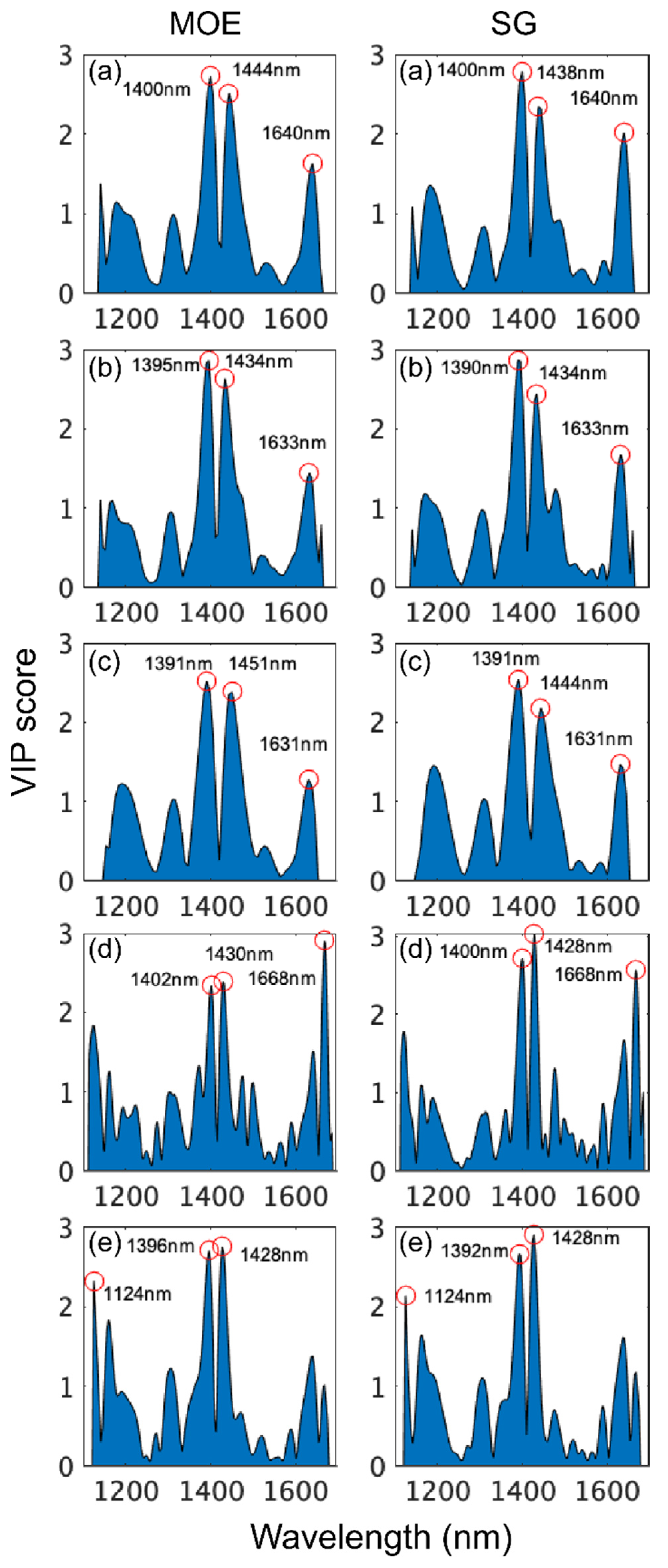
3.3. Calibration/Prediction—MOE and SG Using 1100–1700 nm

The calibration and prediction performance for MOE and SG models obtained using 1100–1700 nm are summarized by instrument in

Table 4. Calibration and test results using SNV and second derivative (segment: 5; gap: 0) treated spectra and limited to the wavelength range 1100–1700 nm with manually fixed latent variables (LVs) to be six.

Device Name	MOE (GPa)				SG
	R2cv	RMSEcv	R2test	RMSEtest	R2cv	RMSEcv	R2test	RMSEtest
SWIR-HSI-I	0.68	1.54	0.75	1.36	0.64	0.03	0.44	0.04
SWIR-HSI-II	0.67	1.55	0.73	1.42	0.69	0.03	0.31	0.04
SWIR-HSI-III	0.61	1.7	0.43	2.06	0.60	0.04	0.25	0.05
NIR-SPECT	0.67	1.55	0.64	1.65	0.61	0.04	0.31	0.04
NIR-HSI	0.79	1.24	0.81	1.18	0.73	0.03	0.43	0.04

. The NIR-HSI camera again provided the best calibration and prediction results for MOE with the SWIR-HSI-I camera and SWIR-HSI-II cameras the next best. The other instruments all had R²_cv greater than 0.61. For SG, the NIR-HSI camera gave the highest R²_cv followed by the SWIR-HSI-I and SWIR-HSI-II cameras. NIR spectra obtained using the SWIR-HSI-I and NIR-HSI cameras provided the best prediction statistics. Overall, the prediction accuracies of most models decreased compared to those reported in Section 3.2, and the SWIR-HSI-III camera provided the weakest MOE and SG predictions.

The examination of VIP scores for the models obtained for the different instruments using wavelengths from 1100 to 1700 nm revealed that the most important regions for MOE and SG model building were from 1390 to 1402 nm and from 1428 to 1451 nm with both regions arising from first overtone CH and OH bond vibrations (Figure 7). There was some variation amongst instruments regarding the remaining important wavelengths. MOE and SG models based on SWIR-HSI-I and SWIR-HSI-III data utilized 1630 to 1640 nm (first overtone OH stretching vibration) and the MOE calibration based on SWIR-HSI-II spectral data utilized 1391 nm and 1631 nm for the calibration of MOE and SG, respectively. The remaining important wavelengths were 1124 nm (NIR-HSI, MOE and SG) and a first overtone CH stretch at 1668 nm (NIR-SPECT both properties).

Table 5. Band assignments for stiffness (MOE) and specific gravity (SG) partial least squares (PLS) calibrations based on three SWIR-HSI cameras, one NIR-HSI camera and a benchtop NIR spectrometer. Wavelength range limited to 1100–1700 nm.

Identified Wavelengths (nm)	Band Location (nm)	Bond Vibration	Wood Component
1124 (MOE, SG)	NA
1190 (MOE)	1188–1195	2nd OT C-H str.	Lignin/(cellulose)
1390–1402 (MOE, SG)	1386	1st OT O-H str.	None specified
		1st OT C-H str. + C-H def.
1428–1451 (MOE, SG)	1428	1st OT O-H str. + H2O	Amorphous cellulose
	1440	1st OT C-H str. + C-H def.	Lignin
	1447	1st OT O-H str.	Lignin
	1448	1st OT O-H str.	Lignin/extractives
1630–1640 (MOE, SG)	1632	1st OT O-H str.	Cellulose
1668 (MOE, SG)	1666	1st OT C-H str.	Hemicellulose
	1668	1st OT Car-H str.	Extractives
	1672–1677	1st OT Car-H str.	Lignin

Note—NA: no vibration specific to wood component assigned, OT: overtone, str.: stretching vibration, def.: deformation vibration, +: combination band; ar: aromatic; t.a.: tentative assignment.

provides a summary of wavelength assignments. For models based on 1100–1700 nm, all but one wavelength (1124 nm) were assigned to specific wood component bond vibrations, indicating that the models in this region relied more heavily on recognized wavelengths.

4. Conclusions

Near infrared spectral data were collected for one-hundred Douglas-fir (Pseudotsuga menziesii) samples using three SWIR-HSI cameras, a NIR-HSI camera with a wavelength range limited to 1100–1700 nm and a benchtop spectrometer. The PLS model calibration/prediction performance based on the NIR data was compared for stiffness (MOE) and specific gravity (SG). Overall, the MOE models were better than those for SG with the NIR-HSI camera providing the best MOE models, whereas for SG models, two SWIR-HSI cameras and the NIR-HSI camera provided data that gave similar results. Examination of variable importance in projection (VIP) scores revealed models based on the SWIR-HSI cameras heavily favored wavelengths greater than 1900 nm (arising from CH and OH combination vibrations), suggesting that wavelengths less than 1900 nm have variation that is not as great or possibly not as strongly related to variation in wood properties, and they are overshadowed in the model building process. In comparison, NIR-his-based models relied on first overtone CH and OH bond vibrations. The benchtop spectrometer never achieved the best calibration/prediction accuracy, likely indicating that the spectra that were collected did not represent the transverse surface of the examined samples as well as those obtained by the HSI cameras.

The results presented confirm an excellent suitability of hyperspectral imaging for the prediction of SG and MOE of lumber specifically and the wood industry in general. However, the limited number of samples does not guarantee the universal application of this solution at this stage of development. The model presented can be iteratively improved by adding additional samples to both the calibration and validation spectral datasets.

References

1. Schimleck, L.R.; Tsuchikawa, S. Application of NIR spectroscopy to wood and wood derived products. In The Handbook of Near-Infrared Analysis, 4th ed.; Ciurczak, E.W., Igne, B., Workman, J., Burns, D.A., Eds.; CRC Press: Boca Raton, FL, USA, 2021; Chapter 37; pp. 759–780. [Google Scholar]
2. Meder, R.; Thumm, A.; Marston, D. Sawmill trial of at-line prediction of recovered lumber stiffness by NIR spectroscopy of Pinus radiata cants. J. Near Infrared Spectrosc. 2003, 11, 137–143. [Google Scholar]
3. Thumm, A.; Meder, R. Stiffness prediction of radiata pine clearwood test pieces using near infrared spectroscopy. J. Near Infrared Spectrosc. 2001, 9, 117–122. [Google Scholar]
4. Fujimoto, T.; Kurata, Y.; Matsumoto, K.; Tsuchikawa, S. Feasibility of near-infrared spectroscopy for online multiple trait assessment of sawn lumber. J. Wood Sci. 2010, 56, 452–459. [Google Scholar] [CrossRef]
5. Kobori, H.; Inagaki, T.; Fujimoto, T.; Okura, T.; Tsuchikawa, S. Fast online NIR technique to predict MOE and moisture content of sawn lumber. Holzforschung 2015, 67, 329–335. [Google Scholar]
6. Burger, J.; Gowen, A. Data handling in hyperspectral image analysis. Chemom. Intell. Lab. Syst. 2011, 108, 13–22. [Google Scholar] [CrossRef]
7. Manley, M. Near-infrared spectroscopy and hyperspectral imaging: Non-destructive analysis of biological materials. Chemical Soc. Rev. 2014, 43, 8200–8214. [Google Scholar]
8. Mishra, P.; Asaari, M.S.M.; Herrero-Langreo, A.; Lohumi, S.; Diezma, B.; Scheunders, P. Close range hyperspectral imaging of plants: A review. Biosyst. Eng. 2017, 164, 49–67. [Google Scholar]
9. Elmasry, G.; Kamruzzaman, M.; Sun, D.W.; Allen, P. Principles and applications of hyperspectral imaging in quality evaluation of agro-food products: A review. Crit. Rev. Food Sci. Nutr. 2012, 52, 999–1023. [Google Scholar]
10. Liu, Y.W.; Pu, H.B.; Sun, D.W. Hyperspectral imaging technique for evaluating food quality and safety during various processes: A review of recent applications. Trends Food Sci. Technol. 2017, 69, 25–35. [Google Scholar]
11. Jones, P.D.; Schimleck, L.R.; So, C.-L.; Clark, A.; Daniels, R.F. High resolution scanning of radial strips cut from increment cores by near infrared spectroscopy. IAWA J. 2007, 28, 473–484. [Google Scholar] [CrossRef]
12. Fernandes, A.; Lousada, J.; Morais, J.; Xavier, J.; Pereira, J.; Melo-Pinto, P. Comparison between neural networks and partial least squares for intra-growth ring wood density measurement with hyperspectral imaging. Comput. Electron. Agric. 2013, 94, 71–81. [Google Scholar] [CrossRef]
13. Fernandes, A.; Lousada, J.; Morais, J.; Xavier, J.; Pereira, J.; Melo-Pinto, P. Measurement of intra-ring wood density by means of imaging VIS/NIR spectroscopy (hyperspectral imaging). Holzforschung 2013, 67, 59–65. [Google Scholar] [CrossRef]
14. Ma, T.; Inagaki, T.; Tsuchikawa, S. Calibration of SilviScan data of Cryptomeria japonica wood concerning density and microfibril angles with NIR hyperspectral imaging with high spatial resolution. Holzforschung 2017, 71, 341–347. [Google Scholar] [CrossRef]
15. Ma, T.; Inagaki, T.; Tsuchikawa, S. Non-destructive evaluation of wood stiffness and fiber coarseness, derived from SilviScan data, via near infrared hyperspectral imaging. J. Near Infrared Spectrosc. 2018, 26, 398–405. [Google Scholar] [CrossRef]
16. Haddadi, A.; Burger, J.; Leblon, B.; Pirouz, Z.; Groves, K.; Nader, J. Using near-infrared hyperspectral images on subalpine fire board. Part 1: Moisture content estimation. Wood Mater. Sci. Eng. 2015, 10, 27–40. [Google Scholar] [CrossRef]
17. Haddadi, A.; Burger, J.; Leblon, B.; Pirouz, Z.; Groves, K.; Nader, J. Using near-infrared hyperspectral images on subalpine fire board. Part 2: Density and basic specific gravity estimation. Wood Mater. Sci. Eng. 2015, 10, 41–56. [Google Scholar] [CrossRef]
18. Schimleck, L.; Dahlen, J.; Yoon, S.-C.; Lawrence, K.; Jones, P. Prediction of Douglas-fir lumber properties: Comparison between a benchtop near-infrared spectrometer and hyperspectral imaging system. Appl. Sci. 2018, 8, 2602. [Google Scholar] [CrossRef] [Green Version]
19. Meder, R.; Meglen, R.R. Near infrared spectroscopic and hyperspectral imaging of compression wood in Pinus radiata D. Don. J. Near Infrared Spectrosc. 2012, 20, 583–589. [Google Scholar] [CrossRef]
20. Fujimoto, T.; Numa, T.; Kobori, H.; Tsuchikawa, S. Visualisation of spatial distribution of moisture content and basic density using near-infrared hyperspectral imaging method in sugi (Cryptomeria japonica). Int. Wood Prod. J. 2015, 6, 46–48. [Google Scholar] [CrossRef]
21. Defoirdt, N.; Sen, A.; Dhaene, J.; De Mil, T.; Pereira, H.; Van Acker, J.; Bulcke, J.V.D. A generic platform for hyperspectral mapping of wood. Wood Sci. Technol. 2017, 51, 887–907. [Google Scholar] [CrossRef]
22. Thumm, A.; Riddell, M. Resin defect detection in appearance lumber using 2D NIR spectroscopy. Eur. J. Wood Wood Prod. 2017, 75, 995–1002. [Google Scholar] [CrossRef]
23. Mora, C.R.; Schimleck, L.R.; Yoon, S.C.; Thai, C.N. Determination of basic density and moisture content of loblolly pine wood disks using a near infrared hyperspectral imaging system. J. Near Infrared Spectrosc. 2011, 19, 401–409. [Google Scholar] [CrossRef]
24. Kobori, H.; Gorretta, N.; Rabatel, G.; Bellon-Maurel, V.; Chaix, G.; Roger, J.M.; Tsuchikawa, S. Applicability of Vis-NIR hyperspectral imaging for monitoring wood moisture content (MC). Holzforschung 2013, 69, 307–314. [Google Scholar] [CrossRef]
25. Chen, J.; Li, G. Prediction of moisture content of wood using Modified Random Frog and Vis-NIR hyperspectral imaging. Infrared Phys. Techn. 2020, 105, 103225. [Google Scholar] [CrossRef]
26. Ma, T.; Inagaki, T.; Tsuchikawa, S. Rapidly visualizing the dynamic state of free, weakly, and strongly hydrogen-bonded water with lignocellulosic material during drying by near-infrared hyperspectral imaging. Cellulose 2020, 27, 4857–4869. [Google Scholar] [CrossRef]
27. Ma, T.; Schimleck, L.; Inagaki, T.; Tsuchikawa, S. Rapid and nondestructive evaluation of hygroscopic behavior changes of thermally modified softwood and hardwood samples using near-infrared hyperspectral imaging (NIR-HSI). Holzforschung 2021, 75, 345–357. [Google Scholar] [CrossRef]
28. Stefansson, P.; Thiis, T.; Gobakken, L.; Burud, I. Hyperspectral NIR time series imaging used as a new method for estimating the moisture content dynamics of thermally modified Scots pine. Wood Mater. Sci. Eng. 2021, 16, 49–57. [Google Scholar] [CrossRef]
29. Thumm, A.; Riddell, M.; Nanayakkara, B.; Harrington, J.; Meder, R. Near infrared hyperspectral imaging applied to mapping chemical composition in wood samples. J. Near Infrared Spectrosc. 2010, 18, 507–515. [Google Scholar] [CrossRef]
30. Thumm, A.; Riddell, M.; Nanayakkara, B.; Harrington, J.; Meder, R. Mapping within-stem variation of chemical composition by near infrared hyperspectral imaging. J. Near Infrared Spectrosc. 2016, 24, 605–616. [Google Scholar] [CrossRef]
31. Colares, C.J.G.; Pastore, T.C.M.; Coradin, V.T.R.; Marques, L.F.; Moreira, A.C.O.; Alexandrino, G.L.; Poppi, R.J.; Braga, J.W.B. Near infrared hyperspectral imaging and MCR-ALS applied for mapping chemical composition of the wood specie Swietenia macrophylla King (Mahogany) at microscopic level. Microchem. J. 2016, 124, 356–363. [Google Scholar] [CrossRef]
32. Burud, I.; Gobakken, L.R.; Flø, A.; Kvaal, K.; Thiis, T.K. Hyperspectral imaging of blue stain fungi on coated and uncoated wooden surfaces. Int. Biodeter. Biodegr. 2014, 88, 37–43. [Google Scholar] [CrossRef]
33. Agresti, G.; Bonifazi, G.; Calienno, L.; Capobianco, G.; Lo Monaco, A.; Pelosi, C.; Picchio, R.; Serranti, S. Surface investigation of photo-degraded wood by colour monitoring, infrared spectroscopy, and hyperspectral imaging. J. Spectrosc. 2013, 2013, 380356. [Google Scholar] [CrossRef]
34. Smeland, K.A.; Liland, K.H.; Sandak, J.; Sandak, A.; Gobakken, L.R.; Thiis, T.K.; Burud, I. Near infrared hyperspectral imaging in transmission mode: Assessing the weathering of thin wood samples. J. Near Infrared Spectrosc. 2016, 24, 595–604. [Google Scholar] [CrossRef] [Green Version]
35. Sandak, A.; Burud, I.; Flø, A.; Thiis, T.; Gobakken, L.; Sandak, J. Hyperspectral imaging of weathered wood samples in transmission mode. Int. Wood Prod. J. 2017, 8 (Suppl. 1), 9–13. [Google Scholar] [CrossRef] [Green Version]
36. Inagaki, T.; Mitsui, K.; Tsuchikawa, S. Visualisation of degree of acetylation in beechwood by near infrared hyperspectral imaging. J. Near Infrared Spectrosc. 2015, 23, 353–360. [Google Scholar] [CrossRef]
37. Awais, M.; Altgen, M.; Mäkelä, M.; Altgen, D.; Rautkari, L. Hyperspectral near-infrared image assessment of surface-acetylated solid wood. ACS Appl. Bio. Mater. 2020, 3, 5223–5232. [Google Scholar] [CrossRef]
38. Geladi, P.; Eriksson, D.; Ulvcrona, T. Data analysis of hyperspectral NIR image mosaics for the quantification of linseed oil impregnation in Scots pine wood. Wood Sci. Technol. 2014, 48, 467–481. [Google Scholar] [CrossRef]
39. Myronycheva, O.; Sidorova, E.; Hagman, O.; Sehlstedt-Persson, M.; Karlsson, O.; Sandberg, D. Hyperspectral imaging surface analysis for dried and thermally modified wood: An exploratory study. J. Spectrosc. 2018, 2018, 10. [Google Scholar] [CrossRef] [Green Version]
40. Stefansson, P.; Burud, I.; Thiis, T.; Gobakken, L.; Larnøy, E. Estimation of phosphorus-based flame retardant in wood by hyperspectral imaging—A new method. J. Spectr. Imaging 2018, 7, a3. [Google Scholar] [CrossRef] [Green Version]
41. Kanayama, H.; Ma, T.; Tsuchikawa, S.; Inagaki, T. Cognitive spectroscopy for wood species identification: Near infrared hyperspectral imaging combined with convolutional neural networks. Analyst 2019, 144, 6438–6446. [Google Scholar] [CrossRef]
42. Ma, T.; Inagaki, T.; Ban, M.; Tsuchikawa, S. Rapid identification of wood species by near-infrared spatially resolved spectroscopy (NIR-SRS) based on hyperspectral imaging (HSI). Holzforschung 2019, 73, 323–330. [Google Scholar] [CrossRef]
43. Ruano, A.; Zitek, A.; Hinterstoisser, B.; Hermoso, E. NIR hyperspectral imaging (NIR-HI) and μxRD for determination of the transition between juvenile and mature wood of Pinus sylvestris L. Holzforschung 2019, 73, 621–627. [Google Scholar] [CrossRef]
44. Sandak, A.; Sandak, J.; Janiszewska, D.; Hiziroglu, S.; Petrillo, M.; Grossi, P. Prototype of the near-infrared spectroscopy expert system for particleboard identification. J. Spectrosc. 2018, 2018, 11. [Google Scholar] [CrossRef]
45. Sofianto, I.A.; Inagaki, T.; Ma, T.; Tsuchikawa, S. Effect of knots and holes on the modulus of elasticity prediction and mapping of sugi (Cryptomeria japonica) veneer using near-infrared hyperspectral imaging (NIR-HSI). Holzforschung 2019, 73, 259–268. [Google Scholar] [CrossRef]
46. Lestander, T.A.; Geladi, P.; Larsson, S.H.; Thyrel, M. Near infrared image analysis for online identification and separation of wood chips with elevated levels of extractives. J. Near Infrared Spectrosc. 2012, 20, 591–599. [Google Scholar] [CrossRef]
47. Serranti, S.; Gargiulo, A.; Bonifazi, G. The utilization of hyperspectral imaging for impurities detection in secondary plastics. Open Waste Manag. J. 2010, 3, 56–70. [Google Scholar] [CrossRef] [Green Version]
48. Bonifazi, G.; Capobianco, G.; Palmieri, R.; Serranti, S. Hyperspectral imaging applied to the waste recycling sector. Spectrosc. Eur. 2019, 31, 8–11. [Google Scholar] [CrossRef]
49. Xiao, W.; Yang, J.H.; Fang, H.Y.; Zhuang, J.T.; Ku, Y.D. Development of online classification system for construction waste based on industrial camera and hyperspectral camera. PLoS ONE 2019, 14, e0208706. [Google Scholar] [CrossRef] [Green Version]
50. Gosselin, R.; Rodrigue, D.; Duchesne, C. A hyperspectral imaging sensor for on-line quality control of extruded polymer composite products. Comput. Chem. Eng. 2011, 35, 296–306. [Google Scholar] [CrossRef]
51. Dahlen, J.; Jones, P.D.; Seale, R.D.; Shmulsky, R. Mill variation in bending strength and stiffness of in-grade Douglas-fir No. 2 2 × 4 lumber. Wood Sci. Technol. 2013, 47, 1167–1176. [Google Scholar] [CrossRef]
52. Barnes, R.J.; Dhanoa, M.S.; Lister, S.J. Standard normal variate transformation and de-trending of near-infrared diffuse reflectance spectra. Appl. Spectrosc. 1989, 43, 772–777. [Google Scholar] [CrossRef]
53. Williams, P.; Norris, K.H. Near-Infrared Technology in the Agricultural and Food Industries, 2nd ed.; American Association of Cereal Chemists: St. Paul, MN, USA, 2001; pp. 145–169. [Google Scholar]
54. Wold, S.; Johansson, A.; Cochi, M. (Eds.) PLS-Partial Least Squares Projections to Latent Structures; ESCOM Science Publishers: Leiden, The Netherlands, 1993; pp. 523–550. [Google Scholar]
55. Schwanninger, M.; Rodrigues, J.; Fackler, K. A review of band assignments in near infrared spectra of wood and wood components. J. Near Infrared Spectrosc. 2011, 19, 287–308. [Google Scholar] [CrossRef]
Figure 1. Near-infrared (NIR) spectra obtained using 4 hyperspectral cameras (SWIR-HSI-I, -II and -III, and NIR-HIS) and one benchtop spectrometer (NIR-SPECT). The spectra represent an average of individual spectra obtained from the transverse surface 100 Douglas-fir samples.
Foundations 02 00035 g001
Figure 2. Stiffness (MOE) partial least squares (PLS) calibration and prediction results based on spectral data provided by SWIR-HSI-I (a), -II (b) and -III (c), NIR-SPECT (d) and NIR-HSI (e).
Foundations 02 00035 g002
Figure 3. Specific gravity (SG) partial least squares (PLS) calibration and prediction results based on spectral data provided by SWIR-HSI-I (a), -II (b) and -III (c), NIR-SPECT (d) and NIR-HSI (e).
Foundations 02 00035 g003
Figure 4. Stiffness (MOE) and specific gravity (SG) root mean square error (RMSE) plotted against number of latent variables (LVs) for calibration and prediction based on spectral data provided by SWIR-HSI-I (a), -II (b) and -III (c), NIR-SPECT (d) and NIR-HSI (e).
Foundations 02 00035 g004
Figure 5. Contribution rate (%) of latent variables (LVs) to stiffness (MOE) and specific gravity (SG) partial least squares (PLS) calibrations based on spectral data provided by SWIR-HSI-I (a), -II (b) and -III (c), NIR-SPECT (d) and NIR-HSI (e).
Foundations 02 00035 g005
Figure 6. VIP scores of wavelengths used to build stiffness (MOE) and specific gravity (SG) partial least squares (PLS) calibrations based on spectral data provided by SWIR-HSI-I (a), -II (b) and -III (c), NIR-SPECT (d) and NIR-HSI (e).
Foundations 02 00035 g006
Figure 7. VIP scores of wavelengths used to build stiffness (MOE) and specific gravity (SG) partial least squares (PLS) calibrations based on spectral data provided by SWIR-HSI-I (a), -II (b) and -III (c), NIR-SPECT (d) and NIR-HSI (e). Wavelength range limited to 1100–1700 nm.
Foundations 02 00035 g007