Article

Geometric State Sum Models from Quasicrystals

Quantum Gravity Research, Los Angeles, CA 90290, USA
*
Author to whom correspondence should be addressed.
Foundations 2021, 1(2), 155-168; https://doi.org/10.3390/foundations1020011
Submission received: 9 September 2021 / Revised: 8 October 2021 / Accepted: 9 October 2021 / Published: 13 October 2021
(This article belongs to the Special Issue Advances in Fundamental Physics)

Abstract

:
In light of the self-simulation hypothesis, a simple form of implementation of the principle of efficient language is discussed in a self-referential geometric quasicrystalline state sum model in three dimensions. Emergence is discussed in the context of geometric state sum models.

1. Introduction

The self-simulation hypothesis (SSH) [1] posits that emergence is a core element in the engine of reality, down to the underlying code—considering spacetime and particles as secondary or emergent from this code. In 1938, Dirac [2] addressed the internal structure of the electron and how it affects the spacetime structure itself. Feynman later evolved this thinking to point out that a point of spacetime is like a computer, which lead Finkelstein to propose that reality is a code in action in his 1969 spacetime code paper [3]. Wheeler later wrote an interesting synthesis of this with ideas like the participatory universe as a self-excited circuit, law without law and it from bit [4,5,6]. Second test edit. This information theoretic line of thinking can lead to many ways of addressing the conundrum of quantum gravity and unification physics problems. We focus here on the specific perspective that a notion of pre-spacetime code or language in action leads to the physics and metaphysics idea of reality as a self-simulation [7,8,9] and requires a new principle to drive the evolution—the principle of efficient language (PEL) [1,7,9,10,11].
To address emergence of physical observables from an information theoretic framework governed by the PEL, we need to set up a concrete, constrained and rigorous mathematical substrate. We will consider the Three-Dimensional Penrose tiling quasicrystal (3DPT), also known as Amman or Ammann-Kramer-Neri tiling, projected from the Z 6 lattice [12,13,14]—a generalization of the two-dimensional Penrose tiling [15]. On this point set and associated tilings, we implement a state sum model [16,17], where the states are given by objects inherent in the quasicrystalline geometry. We consider geometric realism discussed in Section 2 as a new paradigm for state sum models following Einstein’s program of geometrization of physics [18]. As we will see, quasicrystals are a natural substrate for geometric realism, where self-referential geometric symbols [1,19] are given from first principles for both kinematics and dynamics. Details on quasicrystals will be presented in Section 3. Essentially, quasicrystalline structures [20,21,22,23,24] are structures that exhibit a new kind of order—aperiodic order—which lies between disorder and periodicity. Statistical or quantum mechanical models defined on lattices can be generalized in a straightforward manner to quasicrystals [25]. The choice of Z 6 root lattice and its associated 3DPT quasicrystal provides a toy model for the conformal symmetry associated with the D 6 root system and the grand unified gauge theory associated with the exceptional Lie algebra E 8 . Both D 6 and E 8 have similar quasicrystals associated with them [26,27,28]. The gauge symmetry represented in the root system is transformed to a 3D quasicrystal network, working as a toy model for quasicrystalline pre-spacetime code.
Quasicrystals come with a natural non-local structure called an empire [29,30,31,32], which can be considered as their defining property. The geometrical state sum model (GSS) proposed will make use of the concept of empire overlaps (called hits in this paper) built upon the rules driving the dynamics, which we will discuss in Section 4. One element that implements the PEL is that an empire position can save resources in the GSS evolution.
A simple implementation of GSS is given in Section 4.1 with a new kind of cellular automaton game of life, where different patterns emerge. Those patterns then act back on the more general GSS model in the form of observables discussed in Section 4.2. In Section 5, we conclude with some discussion about the notion of emergence within a GSS model that implements the PEL.

2. Geometric Realism

The construction of general relativity (GR) marked a breakthrough for the so-called program of geometrization of physics [18], which basically says that one should start with geometry to understand the physical world—there should be a one-to-one correspondence between physical quantities and geometric objects. Modern physics, starting with Einstein himself, follows a path to apply that idea to generalize GR by going beyond Riemannian manifolds (adding to the usual curvature variable, the torsion and nonmetricity variables). This is in essence Riemann’s program as a unified view of geometry. Some variations of this approach include elements from Klein’s program, which focus on symmetries and their associated groups. However, there is another path that we will consider in light of recent developments in theoretical physics, which brings the lesser known geometric program view of Fedorov/Delone that can address both local and global geometry when considering discrete systems [21]. For example, a problem that can be easily solved by this program is which shapes tile space and how. The idea is that regular point systems are determined by local settings. Global regularity results from the structure of local configurations.
Consider a clear route to the quantization of GR that is given by loop quantum gravity (LQG) [33], where the classical 4-dimensional manifold is foliated in 3-dimensional (3D) spacelike surfaces and the metric field g μ ν is decomposed in terms of connections and tetrads, which, in the 3D foliation, reduces to 3D-connection and the triad field. Then the connection and the triad are promoted to operators in a Hilbert space. This quantization procedure leads to the result that the main kinematic objects are spin network states spanning the Hilbert space. The dynamics can be achieved by the usual path integral procedure and leads to spin foam transition amplitudes. These objects can be described graph-theoretically with S U ( 2 ) -spin quantum numbers labeling the edges of the graphs and another group or algebraic S U ( 2 ) data at the vertices. The spin foam path integral of quantum gravity can be understood as a sum over spin network states. In summary, the main object after the path integral quantization of GR is a sum over states of the quantum geometry. In fact, this formulation is a cornerstone of modern physics. Making use of the similarity of the path integral in quantum field theory and the partition function in statistical mechanics [34], many concrete computations of physical observable with different models, from Ising models to lattice gauge theory, condensed matter systems [35], and quantum gravity, is done with a state sum over discrete lattices or graphs. So, the other path to geometrization of physics is to address the geometry of state sum models at the quantum or statistical mechanics regime.
Geometric realism will dictate for us that the labels, for example a spin state ± 1 , that appear in those graphs, quasicrystals or lattices, must have a one-to-one correspondence with the underlying discrete geometry, in our case, the quasicrystal one. That is, the labels are directly related to the geometric building block of tilings. To be more concrete, let us consider the state sum object
W Δ ( s b ) = N Δ s e A e ( s ) v A v ( s ) ,
In spin foam models or some lattice gauge models, W Δ ( s b ) is called the quantum transition amplitude, or the partition function Z Δ in some Ising like models where one sum also over the boundary states s b . In Equation (1), N Δ is a normalization constant that depends on the discretization Δ. There is weight or amplitude (Weight if W Δ is considered as a partition function or quantum amplitudes in a path integral picture.) A e for each edge of Δ and weight or amplitude A v for each vertex. The sum goes over all the allowed configurations of states s. Usually A e and A v are built from the group and algebraic theoretic implementation of symmetries involved in the specific problem. Geometric realism requires that A e and A v are built from geometry of Δ.
Let us consider some examples of standard state sum models:
  • Ising models
The Ising model, constructed over a lattice Δ can be described using only weights A e given by
A e = e β g s ( e ) g t ( e ) 1
with the sum over spin states s = ± 1 , g s ( e ) representing the spin at the starting vertex and g t ( e ) representing the spin at the end vertex of every edge e. The β coupling constant is proportional to the inverse of temperature. General Ising models can be achieved by allowing the states, s, to take values in a large range of integers 0 , 1 , . . . , n . Further generalization can be considered by allowing the edge weights to locally vary as a general function of the states g s ( e ) g t ( e ) 1 , A e = f ( g s ( e ) g t ( e ) 1 ).
  • Lattice gauge theory (LGT):
LGT gives a non-perturbative formulation of the path integral quantization of gauge theories such as the standard model of particle physics. With LGT one gives up on Lorentz symmetry and works with gauge symmetries at the vertices of the lattice Δ. Gauge invariant quantities are given by Wilson loops made up of edges around a two dimensional face of Δ, g f = e f g e . For continuous groups of symmetry, the sum in Equation (1) is converted on an integral that goes over the infinite of group elements (gauge) symmetry g e and the products of amplitudes on edges and vertices are converted to a product over faces
A f = f ( h f )
where the amplitude functions A f are class functions on the group of symmetry ( f ( g h g 1 ) = f ( h ) ). The explicit form of the function f depends on the specific gauge symmetry model. For example, for Yang-Mills theory, is given by
A f = e β f R t r ( U ( h f ) )
where U is a unitary finite dimensional matrix representation of the group, β here, is a coupling constant. Another example is given by topological models where A f takes the simpler form
A f = δ ( h f )
where the delta function δ is taken with respect to the group measure.
  • Spin foam
In spin foam models, Δ is a triangulation of spacetime manifold or its dual. Spin foam models also have amplitudes associated with faces (or edges), usually give by Equation (5), but also amplitudes A v associated to vertices and constructed from more complicated group invariant objects. In LQG, the group of symmetry is given by the little group ( S U ( 2 ) ) of spacetime symmetries ( S L ( 2 , C ) ). A generalization of spin foam for quantum gravity is to include color charge symmetry ( S U ( 3 ) ), within the weights A e and A v in Equation (1). This can be done by defining the weights from invariants of S U ( 2 ) × S U ( 3 ) [17]. When W Δ ( s b ) depends only on the boundary states, the spin foam is topological and the amplitudes are constructed from topological invariants [16].
State sum models are built from algebraic and group-theoretic elements. Even the simple Ising model can be understood as a discrete Z 2 model. The underlying group and algebraic structures have a geometric correspondence. Geometric realism demands the values on the GSS to come from the geometry, more concretely from tiling of Δ, which, for the specific model presented in next sections, will be a 3D quasicrystal. The states, coupling constants, potentials, weights and amplitudes themselves, will be determined by geometric objects as lengths, volumes and volumetric intersections.

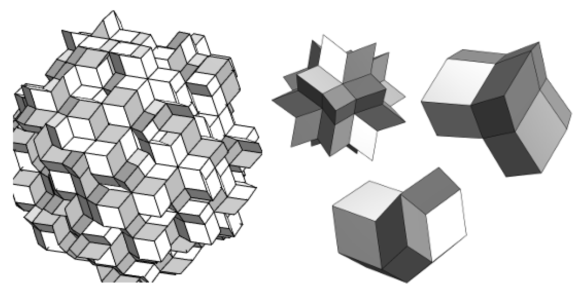
3. Kinematics: The 3D Quasicrystal, Empire and Hits

The construction of the quasicrystal of interest here, the 3DPT, will make use of the canonical cut-and-project method [12,21]. To construct the 3DPT, Δ, we consider the canonical hypercubic lattice Z 6 in Euclidean space R 6 . Let ε be an irrational 3-dimensional subspace of R 6 and ε be its orthogonal complement. Let P be the orthogonal projector onto ε and P onto ε . Now we fix a compact subset K of ε , called the cut-window. The canonical choice for the cut-window is the projection of the Voronoi cell of Z 6 to ε . The Voronoi cell contains one lattice point, which lies at its center. Unlike the unit cells of lattices, these cells are unique and their symmetry groups are the stabilizer groups of the lattice points. The 3DPT quasicrystal Δ is constructed by projecting points λ Z 6 to ε , P ( λ ) , such that P ( λ ) lies inside K, the acceptance domain. Z 6 lattice points are connected by the unit length edges. If two points λ 1 and λ 2 are connected in Z 6 and P ( λ 1 ) and P ( λ 2 ) are accepted, then P ( λ 1 ) and P ( λ 2 ) are connected in Δ. A vertex v i can have different numbers of neighbors, here denoted v i j , with j variating from 1 to the valence of v i (The possible valences for any vertex at some 3DPT are: 4, 6, 8, 10, 12, 14, 16, 20.) The geometric lengths of the connections are labeled as l i j . A tiling T of Δ is a set of possible points and connections given by this procedure. Different tiling configurations can be generated by doing a shift on P ( λ ) in ε before checking if P ( λ ) lies inside K, so-called γ . The shift γ can be used to generate different tilings and it is a continuous parameter that can be used to make the quasicrystal dynamic. A specific 3D tiling T of Δ has two different rhombohedral prototiles building blocks with 10 orientations each. Each vertex v i of one T can be associated to different configurations of prototiles (up to 20 rhombohedral prototile around one vertex v i ). There are 24 possible different vertex types (VT), which appears with different frequencies and valence in a tiling. Most of the 24 VT have valence 20, but those with lower valence appear with more frequency in a tiling. See [12] for the explicit form of VT and its frequencies. A small tiling and 3 of the 3DPT VTs are shown in Figure 1.
The empire is an important property of quasicrystals that arises, in context, within the empire problem [29,30,31,32]. A quasicrystal itself arises in context of the the ancient problem of tiling space in an aperiodic way. To clarify the use of the 3DPT, we can think of Δ generated from K as a possibility point (tiling) space (PS) where points (or VT) can be turned ON or OFF. Or we can think of Δ as the selected points in Z 6 but not projected yet. We are interested in project subsets of those points, the empires, which we define below. The empire problem asks what other vertices or VT of a quasicrystal tiling is forced to be ON if a specific vertex or VT is chosen to be ON—it is projected or actualized. By defining the empire problem and its solutions, one sets the kinematics of a given quasicrystal. For a specific vertex v i in Δ there is associated a specific VT (from the 24 possible ones). We can define a window E K associated to any VT given at some vertex v i , and so, the empire of a point P ( λ i ) of Δ will be the sub-set of Δ such that P ( λ ) lies also inside E. The cut-window K can be volumetric partitioned in sub-windows E, which can overlap. The dynamic quasicrystal can be generated by projecting empires. Empires capture the non-local aspect of quasicrystals [36] in the sense that when a vertex v i is ON, its empire—the whole set of points defined by window E i —is also ON. An additional question can be asked now: If two vertices v 1 and v 2 and their empires are projected, what is the empire overlap between them? The answer is that a measure of the overlap of points sets of different empires is given geometrically by the overlap of empire windows E 1 and E 2 inside the cut-window K. We call this overlap the hit H 12 . Consider the empire given by E 1 to be Δ E 1 and for E 2 to be Δ E 2 , then H 12 = Δ E 1 Δ E 2 or in terms of vertex window polytope intersection for any v i and v j we can compute a normalized measure of overlap by
H i j = I V o l ( E 1 , E 2 ) I V o l ( E 1 )
where I V o l is a function that gives the volume of the intersection of different polytopes, computed here numerically, and if it has only one polytope as input, it returns the volume of that polytope. Computing hits H i j between a VT at v i and different v j positions in one tiling and then changing v i gives a hit map distribution for the specific tiling. One typical example is shown in Figure 2. In what follows we will consider only nearest neighbors H i j .
With the main construction of the 3DPT presented, we can establish that the main kinematics variables of interest are the hits H i j between v i and v j , the length l i j of the connection between v i and v j and the volume V i of the VT polytope associated with v i . We can turn now to the implementation of the dynamics aspects of the GSS W Δ ( s b ) , Equation (1), to be done in the next section.

4. Dynamics: Geometric State Sum Model and the PEL

To implement dynamics of the GSS, we consider the state sum in Equation (1). Following the ideas from the previous sections, the weights A e for an edge linking vertices v i and v j will be given by
A e = l i j H i j ,
where the states given at each edge s i j = H i j are geometric quantities, specifically, volumetric polytope intersections. The length l i j plays the role of the coupling constant or inverse of temperature. We can group these edge states by summing over nearest neighbors v i j
A v i = j l i j H i j .
We will add an additional term to each vertex v i , called the hit potential Y i , which takes into account the PEL by implementing a look-ahead algorithm [37]. Consider a PS tiling T with only the central vertex v c and its empire being ON, which means that the vertex window polytope E v c is being used to select the possible points of the Z 6 that can be projected to the cut-window K. Now we will probe the quasicrystal possibility space △ with random walks of the vertex type at v c using rules based on H i j . So, we start on step 1, with v c and its empire being ON. In step 2, one of the neighbors v c j will be ON according to a non-deterministic rule R ( H i j ) , which we will discuss in Section 4.2. Then we repeat these steps until step N. This defines one animation A 1 . Next, we repeat this procedure, getting a new animation A 2 , and so on until an animation A M , so that we end with M animations, each with N steps. We call these animations possibility space random walks (PRW). The hits potential Y i is defined at each vertex v i as the number of PRWs that use that position. For consistency we will add a volume weight
Y i = V i Y i ,
where V i is the volume of the VT polytope at v i . It encodes the coupling l i j there. The hit potential comes from the idea of minimizing the cost of projection resources to turn ON points on △. The vertices that have more PRWs going over them have more potential to save projection steps to generate animations for the look-ahead algorithm (or here: Look-savings-ahead algorithm). As there are more walks going over those positions they can be part of more possible emergent patterns. The hit potential can be defined from weights of entire animations. We can count hits and associate an integer to one animation A m by counting how many empire vertices the PRW of that animation encounters. These vertices are already ON and don’t need to be turned ON on the PRW. The hits H i j and hit potential Y i associated to a tiling T k define one valid configuration of states given by
W T k = N T k i A v i k Y i k ,
where the index k means that the geometric quantities are computed on the specific tiling T k . The defining object of interest for the GSS is then, in a partition function form,
W Δ = N Δ T k W T k ,
where the sum goes over the different allowed configurations, implemented by finding new allowed tilings. One way to find new tilings, which involves changing only the states H i j and not the couplings l i j or V i , is by using the shift γ . To change the couplings l i j or V i from quasicrystalline first principles, one can use inflation [27], which requires changing the size of the windows. The state sum can also be defined as a transition function for state H a b that fixes a subset of Δ, where H a b can be two disjointed subsets so that maintaining both fixed, and summing over the remaining part, would give the transition function between the states
W Δ ( H a b ) = N Δ T k ( i j / a b ) W T k ,
where the notation ( i j / a b ) indicates that all tilings and their accompanying H i j are generated, but with H a b remaining fixed. This implementation is given by finding values of the shift γ that generate new tilings sharing a fixed configuration.

4.1. A New Kind of Game of Life in Quasicrystals

A concrete implementation of a dynamic GSS Equation (12) is given in the form of a cellular automaton game of life (GoL). In this case we let the quasicrystal tiling space Δ evolve according to local rules, which the same nature of R ( H i j ) we use to generate the hit potential and which we discuss below.
Classical cellular automata are defined on regular lattices. The rules depend on the state of each site and its neighbors. The neighborhood structure looks the same across the lattice. For GoLs [38,39,40,41,42], which have outer totalistic cellular automaton rules, the next state of a site depends only on its current state, and the total number of neighbor sites in certain states. In 2-dimensional quasicrystalline GoLs [43,44,45] the neighborhoods are generalized and not the same for each site, but the dynamics are implemented with similar rules to the original GoL. GoL rules on Penrose tilings still have complex behavior.
The generalization to 3D that implements the GSS model is given by a 5-tuplet G = , T , H , v , R with elements as follows. △ is a 3DPT; T includes the initial tiling condition (where at least one VT is ON) and the set of steps to update △—we usually consider 1000 steps for 5000 3DPT point set; H is the set of states generalized to be a real number between 0 and 1 according to Equation (6); v = v i j are the neighbors of a vertex v i , which vary between 4 and 20—we note that when a vertex is ON the whole VT associated to it is considered to be ON, and also that sometimes we can consider the point set for evolution to have only a specific VT instead of the full quasicrystal point set; R are the new local adapted rules for this kind of GoL. The rules measure empire overlap: If there is too much overlap with ON neighbor VTs then it turns or stays OFF (overpopulation condition); if there is too little overlap it also will be OFF (under-population condition); but if there is the right value of overlap with the mean value of all v i j , then the current vertex will be ON. Good values for the normalized A v i , Equation (8), are found to be between 0.7 and 0.9. We also consider the information entropy associated to hits to drive the evolution as in Equation (14)—in this case the VT will be ON if its information entropy is close enough of the mean of its neighbors, which are ON (one additional option with this kind of GoL is that due to the non-local properties of empires we can allow the rules to be applied to the whole quasicrystal and not only with the connected vertices of a VT, which we will leave for future investigations).
These dynamics lead to different emergent patterns, most of which are oscillation patterns as in Figure 3. There are also different kinds of propagation as in Figure 4. However, varying the rules opens up possibilities of more complex dynamics, which are open for future systematic investigations, but which may also encounter problems of optimization of image processing.

4.2. GSS Observables and Emergence

In light of more general dynamics, we can interpret Equation (12) as one observable on a GSS model. It is a fixed pattern over the space of geometric states. The specific emergent pattern and its properties can be addressed with Equation (12). The hit potential Y i can, in fact, be considered as derived from one observable VT that is ON and that is following a family of PRWs. Let us consider the rules R ( H i j ) in this context. The rules are used to guide the random walks to probe the possibility space and then define the hit potential. What is moving in the quasicrystal, or, what are those VT, which are being turned ON or OFF (being projected/actualized or not)? A GSS model aims to describe pre-spacetime physics—the Planck scale quantum gravity regime. This regime is considered to have the concept of holographic matter [46,47,48,49], which is proportional to information entropy
| I v i I v j | = Δ I i j = α m ,
with α a constant of proportionality and m the mass crossing some horizon. In this Planck scale regime picture, each connection is considered to be crossing a holographic horizon and information is the stuff flowing between horizons and to be conserved. The local information entropy is given by
I i = j P i j l o g P i j
with P i j = H i j N i . Different rules can be implemented under I. The above motivation leads us to the notion of local conservation of I. We simply let the PRW, starting at the center of a tiling, be guided by a probability distribution constructed by choosing each successive position from a local subset whose values of I are within some selected range of the current value of I, which sets the non deterministic look-saving-ahead algorithm. The resultant hit potential Y ( r ) as a function of the distance from the center is given in Figure 5 for 1000 animations over 1000 steps.
The specific form presented in Figure 5 has a mean value that drops with the inverse of distance away from the center but with a Gaussian contribution close to the center. In general its form depends on the distribution of VTs on a specific tiling, the local rules and random walk properties. We can also consider an additional second PRW starting at a different position and allow the Y ( r ) to count overlap between the two walks—a synergistic effect [50] on the whole emergent hit potential not accounted for on the underlying GoL. See Figure 6.
Note that we can use the PRWs to evolve Δ determining H, v and even R of the GoL G . We can also allow local rules at site i to be determined from the full weights A v i Y i . This generates a more sophisticated stratified recursive game
G n + 1 = G ( G n ) .
As a result of the GSS evolution, we consider a candidate for an order parameter, which is analogous to magnetization in spin systems,
H T ( l ) = 1 N T i 1 N i j H i j ( l i j ) ,
where l represents the length inflation scale that defines l i j . As the cut-window K gets smaller, the points in the projected space P ( λ ) get farther way from each other and in the perpendicular space the points P ( λ ) get closer. l i j and V i get bigger but the intersection of vertex window polytopes in the perpendicular space also gets bigger, approaching 1. As a result, over many inflations, we see that there are two dominant regimes. One is “disordered”, where there is not much overlap of vertex window polytopes and there are more local variations so that the information entropy rules depend on hits. The other regime is “ordered”, where the overlaps approach 1 and therefore the information entropy rules should depend only on the vertex valences and not on hits. See Figure 7.
Different emergent dynamics can be considered. For example, we can set a preferred direction to follow the rules and also consider the central hit potential, which leads to interesting curving path patterns as in Figure 8.
As a further result, we consider an oscillation pattern around the center of a tiling with the large symmetric VT there. There are 12 of these same VTs around the center making the geometry of an icosahedron. In each frame step only one of the 12 VTs is ON. This gives a notion of an emergent quasiparticle (the whole icosahedron) with internal structure (the 12 symmetric VTs). See Figure 9.
With this object we can consider a 4-dimensional dynamic by considering the influence of the empires of those 12 VTs at arbitrary 3D positions on Δ. The oscillation on the 12 VTs plays the role of time. We consider a vertex P ( λ 1 ) around the icosahedron. The VT associated to that position depends on the γ tiling T k , V T 1 k = V T ( P ( λ 1 ) ) . By shifting the projections by specific γ values, we can change tiling k and V T 1 k , preserving the oscillating icosahedron pattern at the center. Figure 10 shows the cut-window K (the large window), the empire vertex window for the icosahedron (the middle window), and the small window limiting the available shifts.
So for each P ( λ 1 ) we compute H i j , where i refers to one of the 12 central VTs and j to V T 1 k . We average this computation over a large number of tilings T k and over 12 cycles of the central icosahedron, getting H ¯ i j , and then we go to a new position. We define the observable of interest to be
O ( l i j ) = log ( l i j H ¯ i j ) ,
which gives a different notion of emergent potential as shown in Figure 11. This one grows with distance while the hit potential drops.
As a last result, we consider how information entropy grows with the number of steps for patterns made of different VTs. We define the hit section ( h s ) to be a certain number of the same VTs within some distance r from the center of some tiling. We compute H i j , where i refers to a certain VT at the center of this tiling and j refers to the same VT at different position p on that tiling, p < r , with j h s ,
I i ( r ) = j h s ( r ) P i j l o g P i j .
The result is that I i ( r ) distinguishes the patterns made of different VTs, which should be proportional to the frequency of appearance of the respective VTs, see Figure 12.

5. Discussions and Outlook

In this paper, we discussed state sum models under geometric realism. The SSH paradigm is looking to understand the emergence of spacetime and matter from a pre-spacetime code that takes into account stratification and recursion. GSS is discussed as a framework in this direction. State sum models implement the principles of locality and superposition. GSS adds geometric realism at the state level and the PEL for dynamics. With the GSS formulation, we made concrete the idea that emergence happens due to structure and not necessarily randomness. In the current implementation, the structure is given by a 3D quasicrystal with aperiodic order projected from a 6-dimensional lattice. By having dynamics where different points can be projected or actualized at different steps with their empires, quasiparticle patterns emerge in a simple GoL simulation as presented in Section 4.1. The patterns that emerge are built from known quasicrystal structures, the VTs. A stratified recursive feedback loop can then be established between, on the one hand, the quasicrystal level of projections, non-local empire overlaps and local information entropy rules and, on the other hand, the emergent level of quasiparticle patterns made of VTs. This is expressed as a potential derived from many evolutions of PRWs going over the underlying quasicrystal points, generating an emergent pattern. Overlap of PRW positions or PRWs and empire vertices is understood as potential optimization; it gives an opportunity to economize resources, which in this case are projections from 6 dimensions to 3 dimensions. This implements the PEL by allowing the simulation to express more emergent patterns over less projection step resources. The PEL is implemented on the structure of PRWs, which are considered here as virtual walks to probe the possibility space of walks. It aims to create “cognitive” structure, as in artificial neural networks, so that the simulation itself can decide the best sequence of movements for the emergent pattern. This kind of structure under the emergence paradigm within complex systems is what is observed in general: The emergent structure, with its new emergent properties, always occurs under the dynamics of a large underlying number of building blocks that have structure governing their dynamic interactions. This is seen from atoms to DNA to neurons to stars and galaxies.
In this work, we investigated some general code theoretic properties of general emergent patterns on the GSS. For future investigations, we aim to derive the physical emergent laws governing the dynamics of the emergent patterns, making more concrete the emergence of spacetime and matter. An important hint in this direction is that the cut-and-project method used to derive the quasicrystal makes clear the connection with the higher dimensional lattices. The main quasicrystals of interest are derived from the so-called root lattices of Lie algebras. Lie algebras and groups are the language of symmetry and so a core element in fundamental physics, as in quantum mechanics. The dynamics derived in this paper can be thought of as a dynamics that tails back to the root system of Lie algebras [17,27], suggesting a generalization from Z 6 to D 6 and E 8 .
One different consideration to be addressed for GSS models is the computational efficiency on current classical computers. The values on usual state sum models come from algebraic or group-theoretic objects. There are more computational costs to obtain the values from the geometry.

Author Contributions

Conceptualization, M.A., F.F. and K.I.; methodology, M.A.; software, M.A. and D.H.; validation, F.F.; formal analysis, M.A.; investigation, M.A., F.F. and D.H.; writing—original draft preparation, M.A.; writing—review and editing, M.A.; visualization, F.F.; supervision, M.A. and K.I.; project administration, K.I.; funding acquisition, K.I. All authors have read and agreed to the published version of the manuscript.

Funding

This research received no external funding.

Acknowledgments

We acknowledge the many discussions had with David Chester, Raymond Aschheim and Richard Clawson and we thank them for their generous feedback in editing discussions.

Conflicts of Interest

The authors declare no conflict of interest.

Abbreviations

The following abbreviations are used in this manuscript:
SSHSelf-simulation hypothesis
PELPrinciple of Efficient Language
3DPT3-Dimensional Penrose Tiling quasicrystal
PELGeometrical State Sum (GSS)
GRGeneral Relativity
LQGLoop Quantum Gravity
3D3-dimensional
LGTLattice Gauge Theory
VTVertex Type
PSPossibility Space
PRWPossibility Random Walk
GoLGame of Life

References

  1. Irwin, K.; Amaral, M.; Chester, D. The Self-Simulation Hypothesis Interpretation of Quantum Mechanics. Entropy 2020, 22, 247. [Google Scholar] [CrossRef] [Green Version]
  2. Dirac, P.A.M. Classical theory of radiating electrons. Proc. Roy. Soc. Lond. A 1938, 167, 148–169. [Google Scholar]
  3. Finkelstein, D. Space-time code. Phys. Rev. 1969, 184, 1261–1279. [Google Scholar] [CrossRef]
  4. Wheeler, J.A. Beyond the Black Hole. In Some Strangeness in the Proportion: A Centennial Symposium to Celebrate the Achievements of Albert Einstein; Woolf, H., Ed.; Addison-Wesley: Reading, MA, USA, 1980. [Google Scholar]
  5. Wheeler, J.A. Hermann Weyl and the Unity of Knowledge. Am. Sci. 1986, 74, 366–375. [Google Scholar]
  6. Wheeler, J.A. Information, physics, quantum: The search for links. In Complexity, Entropy, and the Physics of Information; Addison-Wesley: Boston, MA, USA, 1990. [Google Scholar]
  7. Langan, C.M. The Cognitive-Theoretic Model of the Universe: A New Kind of Reality Theory. Prog. Complex. Inf. Des. 2002, 1, 2–3. [Google Scholar]
  8. Aschheim, R. Hacking Reality Code. FQXI Essay Contest 2011, Category: Is Reality Digital or Analog? Essay Contest (2010–2011), Number 929. Available online: https://fqxi.org/community/forum/category/31417 (accessed on 8 October 2021).
  9. Irwin, K. A New Approach to the Hard Problem of Consciousness: A Quasicrystalline Language of Primitive Units of Consciousness in Quantized Spacetime. J. Conscious Explor. Res. 2014, 5, 483–497. [Google Scholar] [CrossRef]
  10. Irwin, K. The Code-Theoretic Axiom: The Third Ontology. Rep. Adv. Phys. Sci. 2019, 3, 1950002. [Google Scholar] [CrossRef]
  11. Irwin, K.; Amaral, M.M.; Aschleim, R.; Fang, F. Quantum walk on spin network and the golden ratio as the fundamental constant of nature. In Proceedings of the Fourth International Conference on the Nature and Ontology of Spacetime, Varna, Bulgaria, 30 May–2 June 2016; pp. 117–160. [Google Scholar]
  12. Hammock, D.; Fang, F.; Irwin, K. Quasicrystal Tilings in Three Dimensions and Their Empires. Crystals 2018, 8, 370. [Google Scholar] [CrossRef] [Green Version]
  13. Katz, A. Theory of Matching Rules for the 3-Dimensional Penrose Tilings. Commun. Math. Phys. 1988, 118, 263–288. [Google Scholar] [CrossRef]
  14. Takakura, H.; Gomez, C.; Yamamoto, A.; De Boissieu, M.; Tsai, A.P. Atomic structure of the binary icosahedral Yb-Cd quasicrystal. Nat. Mater 2007, 6, 58–63. [Google Scholar] [CrossRef]
  15. Penrose, R. The role of aesthetics in pure and applied mathematical research. Bull. Inst. Math. Appl. 1974, 10, 266–271. [Google Scholar]
  16. Barrett, J.W. State sum models for quantum gravity. arXiv 2000, arXiv:gr-qc/0010050. [Google Scholar]
  17. Amaral, M.; Aschheim, R.; Irwin, K. Quantum Gravity at the Fifth Root of Unity. arXiv 2019, arXiv:1903.10851. [Google Scholar]
  18. Wanas, M.I. The accelerating expansion of the universe and torsion energy. Int. J.Mod. Phys. A 2007, 31, 5709–5716. [Google Scholar] [CrossRef] [Green Version]
  19. Irwin, K. Toward the Unification of Physics and Number Theory. Rep. Adv. Phys. Sci. 2019, 3, 1950003. [Google Scholar] [CrossRef] [Green Version]
  20. Baake, M.; Grimm, U. Aperiodic Order; Cambridge University Press: Cambridge, UK, 2013. [Google Scholar]
  21. Senechal, M.J. Quasicrystals and Geometry; Cambrige University Press: Cambrige, UK, 1995. [Google Scholar]
  22. Levine, D.; Steinhardt, P.J.; Quasicrystals, I. Definition and structure. Phys. Rev. B 1986, 34, 596. [Google Scholar] [CrossRef]
  23. Gardner, M. Extraordinary nonperiodic tiling that enriches the theory of tiles. Sci. Am. 1977, 236, 110. [Google Scholar] [CrossRef]
  24. De Bruijn, N.G. Algebraic theory of Penrose’s non-periodic tilings. Nederl Akad Wetensch Proc. 1981, 84, 1–7. [Google Scholar] [CrossRef] [Green Version]
  25. Grimm, U. Aperiodicity and Disorder-Do They Play a Role? In Computational Statistical Physics: From Billiards to Monte Carlo; Hoffmann, K.H., Schreiber, M., Eds.; Springer: Berlin/Heidelberg, Germany, 2002; pp. 191–210. [Google Scholar]
  26. Elser, V.; Sloane, N.J.A. A highly symmetric four-dimensional quasicrystal. J. Phys. A 1987, 20, 6161–6168. [Google Scholar] [CrossRef]
  27. Chen, L.; Moody, R.V.; Patera, J. Non-crystallographic root systems. In Quasicrystals and Discrete Geometry; Fields Institute Monographs; American Mathematical Society: Providence, RI, USA, 1998; Volume 10. [Google Scholar]
  28. Fang, F.; Irwin, K. An Icosahedral Quasicrystal and E8 derived quasicrystals. arXiv 2016, arXiv:1511.07786. [Google Scholar]
  29. Conway, J.H. Triangle tessellations of the plane. Amer. Math. Mon. 1965, 72, 915. [Google Scholar]
  30. Grunbaum, B.; Shephard, G.C. Tilings and Patterns; W. H. Freeman and Company: New York, NY, USA, 1987. [Google Scholar]
  31. Effinger-Dean, L. The Empire Problem in Penrose Tilings. Bachelor’s Thesis, Williams College, Williamstown, MA, USA, 2006. [Google Scholar]
  32. Fang, F.; Hammock, D.; Irwin, K. Methods for Calculating Empires in Quasicrystals. Crystals 2017, 7, 304. [Google Scholar] [CrossRef] [Green Version]
  33. Rovelli, C.; Vidotto, F. Covariant Loop Quantum Gravity, 1st ed.; Cambridge University Press: Cambridge, UK, 2014. [Google Scholar]
  34. Ortiz, L.; Amaral, M.; Irwin, K. Aspects of aperiodicity and randomness in theoretical physics. arXiv 2020, arXiv:2003.07282. [Google Scholar]
  35. Bahr, B.; Dittrich, B.; Ryan, J.P. Spin foam models with finite groups. J. Grav. 2013, 2013, 549824. [Google Scholar] [CrossRef] [Green Version]
  36. Fang, F.; Paduroiu, S.; Hammock, D.; Irwin, K. Empires: The Nonlocal Properties of Quasicrystals. In Electron Crystallography, Devinder Singh and Simona Condurache-Bota; IntechOpen: London, UK, 2019. [Google Scholar]
  37. Alexander, S.; Cunningham, W.J.; Lanier, J.; Smolin, L.; Stanojevic, S.; Toomey, M.W.; Wecker, D. The Autodidactic Universe. arXiv 2021, arXiv:2104.03902. [Google Scholar]
  38. Gardner, M. Mathematical games—The fantastic combinations of John Conway’s new solitaire game of ‘life’. Sci. Am. 1970, 223, 120–123. [Google Scholar] [CrossRef]
  39. Klein, J. Breve: A 3d environment for the simulation of decentralized systems and artificial life. In Proceedings of the 8th International Conference on Artificial Life, Dortmund, Germany, 14–17 September 2003. [Google Scholar]
  40. Bak, P.; Chen, K.; Creutz, M. Self-organized criticality in the Game of Life. Nature 1989, 342, 780. [Google Scholar] [CrossRef]
  41. Bays, C. Candidates for the game of life in three dimensions. Complex Syst. 1987, 1, 373–400. [Google Scholar]
  42. Couclelis, H. Cellular worlds: A framework for modeling micro—macro dynamics. Environ. Plan. A 1985, 17, 585–596. [Google Scholar] [CrossRef]
  43. Bailey, D.A.; Lindsey, K.A. Game of Life on Penrose Tilings. arXiv 2017, arXiv:1708.09301. [Google Scholar]
  44. Owens, N.; Stepney, S. Investigations of Game of Life Cellular Automata Rules on Penrose Tilings: Lifetime, Ash, and Oscillator Statistics. J. Cell. Autom. 2010, 5, 207–225. [Google Scholar]
  45. Fang, F.; Paduroiu, S.; Hammock, D.; Irwin, K. Non-Local Game of Life in 2D Quasicrystals. Crystals 2018, 8, 416. [Google Scholar] [CrossRef] [Green Version]
  46. Bekenstein, J.D. Black holes and entropy. Phys. Rev. D 1973, 7, 2333–2346. [Google Scholar] [CrossRef]
  47. Verlinde, E. On the origin of gravity and the laws of Newton. J. High Energ. Phys. 2011, 2011, 29. [Google Scholar] [CrossRef] [Green Version]
  48. García-Islas, J.M. Entropic Motion in Loop Quantum Gravity. Can. J. Phys. 2016, 94, 569–573. [Google Scholar] [CrossRef] [Green Version]
  49. Amaral, M.M.; Aschheim, R.; Irwin, K. Quantum walk on a spin network. arXiv 2016, arXiv:1602.07653. [Google Scholar]
  50. Goertzel, B. Toward a Formal Model of Cognitive Synergy. arXiv 2018, arXiv:1703.04361. [Google Scholar]
Figure 1. 3DPT tiling and some VTs.
Foundations 01 00011 g001
Figure 2. A typical hit map for the 3DPT quasicrystal. We consider a list with 1000 points of a 3DPT tiling and compute vertex window polytope overlap between them, Equation (6).
Foundations 01 00011 g002
Figure 3. One 3DPT GoL oscillation pattern. The pattern is a oscillator period 2 and the two frames are shown.
Foundations 01 00011 g003
Figure 4. A recurrent pattern propagation for a 3DPT GoL made mainly from the VTs from Figure 3. (18) show eight frames of the dynamics where the pattern highlighted moves from left to right.
Foundations 01 00011 g004
Figure 5. PRW hit potential.
Foundations 01 00011 g005
Figure 6. PRW hit potential from two patterns evolution starting at different positions with one at origin.
Foundations 01 00011 g006
Figure 7. Average hits H T ( l ) evolution under inflations.
Foundations 01 00011 g007
Figure 8. Evolution considering local information entropy conservation, initial preferred direction and the central hit potential.
Foundations 01 00011 g008
Figure 9. Central icosahedron oscillating pattern.
Foundations 01 00011 g009
Figure 10. Available points for shifts γ presented inside the small window.
Foundations 01 00011 g010
Figure 11. Potential due to composite quasiparticle oscillating at the center of the tiling.
Foundations 01 00011 g011
Figure 12. Information entropy order parameter for different VTn, where the integer n number the 3DPT VTs and we show only 5 of the 24. h s grows different with distance for the different VTs.
Foundations 01 00011 g012
Publisher’s Note: MDPI stays neutral with regard to jurisdictional claims in published maps and institutional affiliations.

