An Intelligent Framework for Crowdsource-Based Spectrum Misuse Detection in Shared-Spectrum Networks

Abstract

Dynamic Spectrum Access (DSA) has emerged as a viable solution to address spectrum scarcity in shared-spectrum networks. In response, the FCC established the Citizens Broadband Radio Service (CBRS) to manage and facilitate shared use of the federal and non-federal spectrum in a three-tiered access and authorization framework. However, due to the open nature of spectrum access and the usually limited coverage of the monitoring infrastructure, enforcing access rights in a shared-spectrum network becomes a daunting challenge. In this paper, we stipulate the use of crowdsourcing as a viable approach to engaging volunteers in spectrum monitoring in order to enforce spectrum access rights robustly and reliably. The success of this approach, however, hinges strongly on ensuring that spectrum access enforcement is carried out by reliable and trustworthy volunteers within the monitored area. To this end, a hybrid spectrum monitoring framework is proposed, which relies on opportunistically recruiting volunteers to augment the otherwise limited infrastructure of trusted devices. Although a volunteer’s participation has the potential to enhance monitoring significantly, their mobility may become problematic in ensuring reliable coverage of the monitored spectrum area. To ensure continued monitoring, inspite of volunteer mobility, deep learning-based models are used to predict the likelihood that a volunteer will be available within the monitoring area. Three models, namely LSTM, GRU, and Transformer, are explored to assess their feasibility and viability to predict a volunteer’s availability likelihood over an extended time interval, in a given spectrum monitoring area. Recurrent Neural Networks (RNNs) such as GRU and LSTM are effective for tasks involving sequential data, where both spatial and temporal patterns matter, which is the focus of volunteer availability prediction in spectrum monitoring. Transformers, on the other hand, excel at handling long range dependencies and contextual understanding. Furthermore, their parallel processing capabilities allows faster training and inference compared to RNN-based models like GRU and LSTM. A simulation-based study is developed to assess the performance of these models, and carry out a comparative analysis of their ability to predict volunteers’ availability to monitor the spectrum reliably. To this end, a real-world trace dataset of volunteers’ location, collected over five years, is used. The simulation results show that the three models achieve high prediction accuracy of volunteers’ availability, ranging from 0.82 to 0.92. The results also show that a GRU-based model outperforms LSTM and Transformer-based models, in terms of accuracy, Root Mean Square Error (RMSE), geodesic distance, and execution time.

1. Introduction

The internet has ushered in a new era in which users’ expectations are high for universal access to multimodal content. Despite unprecedented advances in network communications and wireless technology, spectrum demand continues to outstrip supply, especially in dense areas, where rural and in-building coverage continues to lag. In recent years, various methods have focused on exploring the potential of spectrum sharing to optimize spectrum utilization and meet the rising demands for high-quality mobile experience. Most notable among these developments is the establishment of the Citizens Broadband Radio Service (CBRS) by the Federal Communications Committee (FCC) to facilitate shared federal and non-federal use of the 3550–3700 MHz band [1]. CBRS stipulates the creation of a three-tiered access and authorization framework to accommodate the requirements of the shared federal and non-federal use of the band. This architecture consists of Incumbents in tier 1, Priority Access Licensed (PAL) users in tier 2, and General Authorized Access (GAA) users in tier 3. The spectrum is always available to tier 1 incumbents whenever needed. Tier 2 PAL users are protected from interference by tier 3 GAA users. However, GAA users are neither protected from higher-tier users nor from other GAA users in the same tier.

Although it improves the efficiency of radio spectrum usage, shared access is susceptible to spectrum misuse and abuse that go beyond interference [2,3]. Shared-spectrum networks are likely to be prone to unauthorized users, who can intentionally carry out illicit activities, including violating the interference constraints established by incumbents, transmitting aggressively, both in time and frequency, to gain disproportionate use of the spectrum, and disrupting network operations by violating pre-set spectrum access rules and policies. As the intensity for spectrum sharing increases, so does the rate of access rights violations and anomalous behavior. The ensuing tension underscores the need for reliable enforcement mechanisms to prevent access violation while enabling productive use of scarce spectrum resources. Hence, the success of a spectrum-sharing model depends on the ability to effectively monitor spectrum and enforce spectrum access policy.

Traditional spectrum monitoring usually relies on the deployment of a static infrastructure of high-capability devices [4]. However, the cost of ensuring the necessary channel coverage for reliable access right enforcement may become prohibitive. Focusing on ex-post (punitive) spectrum enforcement in a shared-spectrum wireless environment, the main objective of the paper is to demonstrate the feasibility of a hybrid, cost-effective, crowdsource-based infrastructure to enforce spectrum access policies, efficiently and reliably. The main monitoring component of the hybrid infrastructure is composed of trusted devices, operated by permanently assigned human agents, referred to as sentinels. This monitoring component is augmented with opportunistically recruited human volunteers, equipped with wireless sensing devices, to assist sentinels with monitoring activities. The hybrid infrastructure is designed to ensure adequate coverage, and cost-effective monitoring to detect spectrum access right violations [5,6,7,8].

Performing spectrum monitoring across large geographical areas is a daunting endeavor. This stems from the difficulty to achieve adequate coverage while minimizing cost. Consistent with our proposed infrastructure, a number of research works proposed approaches to harness the potential of crowdsourcing and engage a large number of participants to achieve adequate coverage of large geographical areas. These works focus mainly on recruiting volunteers to achieve optimal coverage of the monitored area. In their selection of volunteers, however, most of these works do not take into consideration the mobility of the recruited spectrum monitors. The movement of volunteers out of a region, when it occurs, may result in reduced coverage of the monitored area. This, in turn, may lead to the exposure of monitored regions to spectrum access violations by intruders.

To ensure sustained coverage, it is critical to accurately estimate the location of a volunteer within a region and effectively estimate their availability within the region. To this end, a region is divided into coverage zones. A suite of integrated, AI-based approaches is then used to predict the likelihood of a volunteer’s availability within a zone for a monitoring interval. A monitoring interval refers to a specified time period over which monitoring is carried out. At the end of each interval, the assignment of volunteers to area coverage is re-evaluated to identify and address coverage gaps, ensuring comprehensive and sustained monitoring across the entire spectrum sharing area. Collectively, these approaches significantly increase the likelihood that volunteers carry out their monitoring assignment consistently and reliably. Mechanisms are also proposed to ensure that standby volunteers are ready to respond immediately to the occurrence of spectrum undercoverage, should such an event occur when the assigned volunteer leaves the enforcement zone. Standby monitors play a critical role in ensuring continuous monitoring and reliable enforcement of regulatory access rights across the monitored region. In essence, standby monitors transform monitoring from a reactive into a proactive process to reduce exposure to anomalous behavior. Ensuring an immediate response to potential spectrum undercoverage significantly increases the effectiveness of spectrum access rights enforcement.

The novelty of the proposed framework resides in its comprehensive approach to spectrum access rights enforcement. The framework also positions mobility prediction as a critical and enabling component, providing the basic tenet for an end-to-end spectrum access rights enforcement infrastructure. Specifically, we: (i) couple zone-level coverage requirements with volunteer selection; (ii) formalize volunteer qualification to reflect their ability for a sustained and reliable coverage, using an aggregate metric that combines the predicted likelihood of a volunteer to be located within a spectrum monitoring zone and their capability to carry out the monitoring task in a sustained and reliable manner; and (iii) quantify how prediction quality impacts enforcement-relevant outcomes, using real-world mobility traces. Furthermore, volunteer selection and assignment mechanisms are proposed to seamlessly engage volunteers in collaborative, interference-free spectrum monitoring activities with sentinels, who typically operate within fixed locations and consistent schedules. Volunteers can respond dynamically and flexibly to monitoring tasks. Rather than imposing specific coverage areas on volunteers, the proposed approach opportunistically aligns spectrum monitoring tasks with volunteers’ planned activities, based on their predictable availability within a region. These assignments are “episodic” in nature, taking into consideration volunteers’ mobility and their inability to commit to long-term monitoring.

The main contributions of the paper are as follows:

• A crowdsourced spectrum access rights enforcement infrastructure to detect potentially enforceable events effectively and reliably.
• A dynamic programming-based approach to determine the minimum number of selected crowdsourced volunteers required to achieve expected coverage threshold, where the spectrum enforcement area is divided into regions and each region is further divided into zones to ensure zone-level coverage.
• A deep learning-based approach to predict which geographic coverage zone a volunteer is likely to occupy at a given time, and uses the model-derived probability combined with coverage to qualify and select crowdsourced volunteers more reliably for spectrum enforcement.

The remainder of the paper is organized as follows: Section 2 discusses some of the works that are relevant to the work presented in this paper. In Section 3, the shared-spectrum monitoring framework is introduced, and its main components are briefly described. In Section 4, the deep learning-based models used to predict the future availability of volunteers are presented. Comparative performance analysis of these models, along with the experimental setup and methodologies used for comparison, are discussed in Section 5. The results of the analysis are presented in Section 6. The conclusions of this paper are highlighted in Section 7.

2. Related Works

A significant body of research works has focused on the design of crowdsourcing frameworks, approaches, and methods to leverage the collective intellect of a crowd and engage experts and stakeholders to work collaboratively in sharing ideas, brainstorming solutions, and advancing knowledge. While most of these crowdsourcing-driven research efforts share common building blocks, the features and context within which the crowdsourcing infrastructure is conceived differ to varying extents. Different topologies for crowdsourcing have been proposed, depending on the type of the crowdsourcing event, collaboration- or competition-based, the intended objectives, the participants’ selection process, and the control of the tasks to achieve the targeted outcomes [9,10,11]. These topologies have been adopted, with varying degrees of success, in various activities and in different communities, including Wikipedia, Youtube, Healthcare, Disaster Management, Citizen Science, Transportation, City Management, Upwork, Gigster, TopCoder, Rainforest QA, Kaggle, GLG, and HackerOne  [12,13,14,15,16].

Several research works have explored the use of crowdsourcing to carry out spectrum monitoring tasks in shared-spectrum wireless networks [17,18]. These research efforts can be broadly classified into two categories based on the objective and main goals of the spectrum monitoring task. In the first category, the focus is on recruiting, motivating, and retaining volunteers. These issues are critical to ensure the sustainability of the crowdsourced monitoring tasks over an extended time. In these works, the proposed approaches to achieve crowdsourcing sustainability rely on auction and the use of different methodologies, including “agent utility”, stable matching, and threshold-driven selection algorithms to recruit volunteers [5,6,7,19,20]. Successful volunteer recruiting usually relies on the strive of volunteers for the “common good” and potential “recognition” of their positive community impact [21]. In the second category, the focus is on detecting spectrum misuse and identifying intruders and access violators. Liu et al. proposed and discussed methods to detect anomalous spectrum usage in DSA networks, using the notion of signal prints and log-scale path loss with changes in log-distance [22]. In [22], an adaptive, Markov decision process-based approach is proposed to detect selfish misuse of bandwidth in 802.11-based wireless networks. In [23], the authors propose a framework for cooperative spectrum sensing, focusing primarily on identifying malicious secondary users based on data agreement and the statistics of consecutive true and false decisions.

One important aspect of crowdsourcing-based detection of spectrum intrusion is an effective incentive mechanism to successfully recruit trustworthy volunteers and reliably and efficiently engage them in the enforcement of spectrum access rights. The incentive choice must cater to diverse volunteers’ capabilities and availabilities. Furthermore, trust must be maintained through a reputation mechanism, which provides the basis to identify and eventually expel corrupt volunteers. Finally, recruiting must be dynamic and adaptive to ensure long-term engagement by allowing new participants to join, while reducing the likelihood of volunteers to drop-off. A variety of methods have been proposed in crowdsourcing frameworks to achieve effective recruitment and engagement of volunteers [24]. Some of these methods use mutual benefit or direct impact on the interests of individual participants for recruiting [25]. Other methods use either financial incentives or benefits to the general population to motivate participation in the crowdsourcing event [26,27,28,29,30]. Recent works on intelligent spectrum management and monitoring in shared wireless networks is dominated by AI-driven sensing, learning-based resource allocation, and new architectures to support large-scale, multi-stakeholder spectrum sharing. In the area of AI-enhanced spectrum monitoring and sensing, deep learning, particularly CNN-based models, is increasingly being used at the sensing and monitoring layer to recognize signals, protocols, and occupancy patterns in dense shared bands [31]. These models are also used to reliably classify coexisting technologies and interference to enhance spectrum utilization and coexistence management in heterogeneous, shared-spectrum networks. To scale monitoring over a wideband spectrum, decentralized deep learning, combined with intelligent reflecting surfaces, has been used to improve cooperative sensing and mitigate high-frequency path loss, while reliably tracking spectrum occupancy [32,33,34]. Furthermore, intelligent resource management frameworks, which combine SVM-based spectrum sensing, CNN-based prediction, and priority-aware spectrum allocation in hierarchical shared frameworks, have been used to improve interference detection reliability and spectrum efficiency, even under strong co-channel interference [35,36]. These works show that intelligent spectrum monitoring and spectrum misuse detection can lead to significant capacity gains for all network stakeholders. AI-based control, based on deep reinforcement learning, has proven to be efficient in managing intelligent spectrum and communication resources, minimizing interference, and optimizing energy efficiency, resulting in significant reductions in interference and primary user collisions [37,38]. Wireless network analytics are proposed as a toolchain for large-scale, largely autonomous spectrum monitoring, integrating measurement, machine learning, and anomaly detection [39,40]. In particular, blockchain-based frameworks, enabled by smart contract approaches, have been proposed to implement spectrum trading and sensing, as a service, without trusted brokers, to improve spectrum efficiency and responsiveness under communication delays [41,42]. Intelligent, proactive monitoring is also used for incumbent protection and security in shared heterogeneous, shared-spectrum environments. AI-driven incumbent protection frameworks and algorithms have been used in collaborative intelligent radio networks to learn and predict incumbent traffic patterns with high accuracy, enabling decentralized spectrum sharing, while guaranteeing protection without centralized coordinators [43]. Proactive spectrum monitoring schemes, which combine jamming-assisted observation with data transmission, significantly outperform passive monitors when tracking suspicious communications in dynamic sharing environments [44,45,46,47,48].

3. Spectrum Access Right Enforcement Framework

As discussed previously in [5,6,7], in shared-spectrum networks, authorized transmitters gain access to an available channel through a local access point located in a geographical spectrum enforcement area, where they currently reside. The use of spectrum frequency by an unauthorized transmitter, thereof referred to as the intruder, constitutes a spectrum access rights violation.

The basic tenet of our approach is that unauthorized spectrum access can be effectively prevented by using a trusted monitoring infrastructure, composed of trusted devices, referred to as sentinels, augmented by highly-qualified crowdsourced volunteers. Sentinels are assumed to have advanced authentication capabilities and are fully dedicated to monitoring spectrum access. Achieving a high level of spectrum misuse detection over extended geographical coverage; however, this is likely to come at the high cost of using a large number of sentinels. To increase coverage and minimize cost, crowdsourcing is used to harness the abundance of peer wireless devices, referred to as volunteers, and strengthen the ability of the trustworthy sentinels to reliably detect unauthorized spectrum access. The volunteers are recruited to join the monitoring infrastructure, based on their capabilities to monitor the spectrum. Approaches to effective selection of the most qualified volunteers in the crowd are discussed in [7,8].

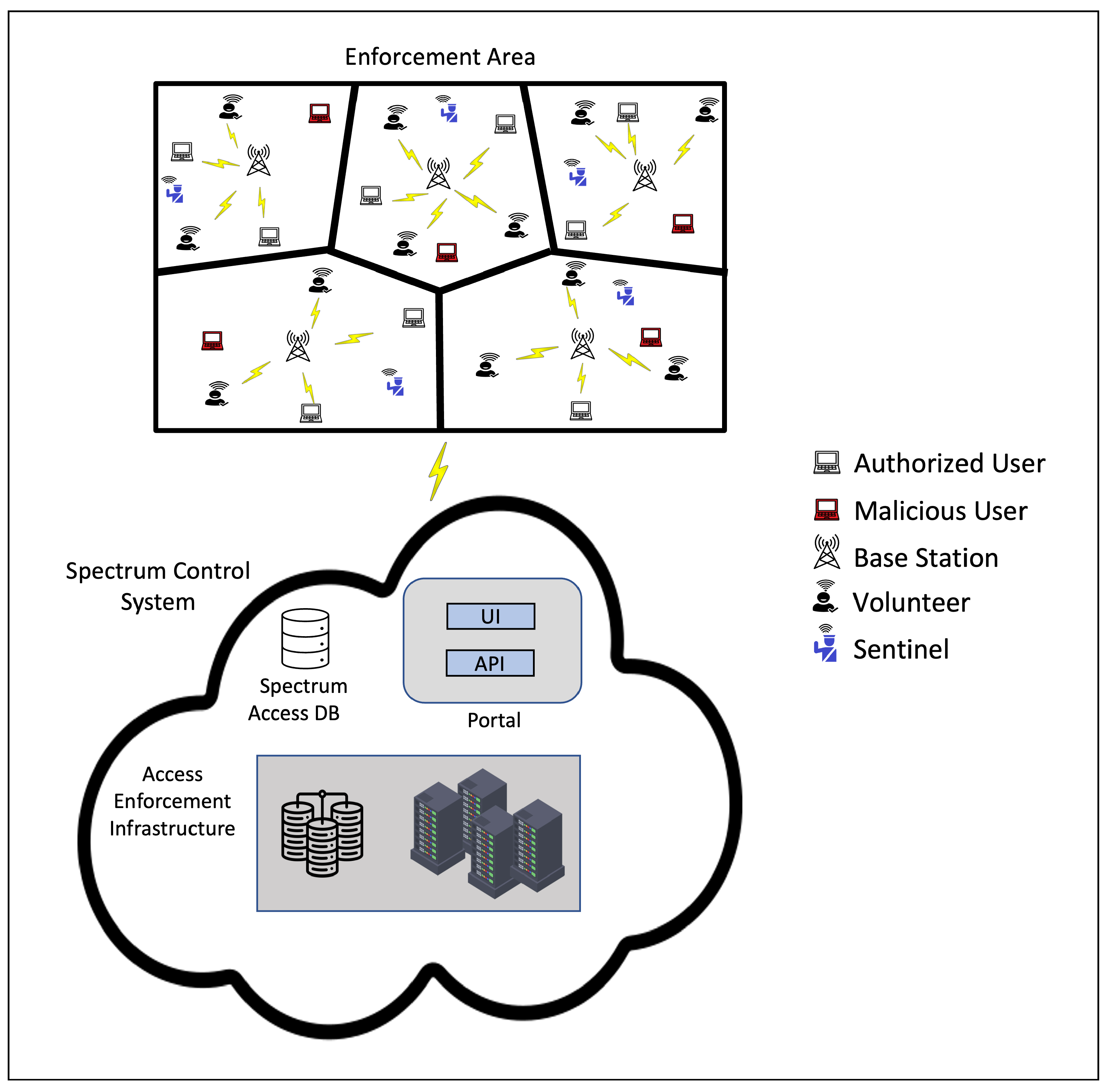
A cloud-based centralized Spectrum Control System (SCS) is used to select crowdsourced volunteers to monitor the spectrum in the enforcement area. As shown in Figure 1, the SCS consists of: (i) a portal for collecting spectrum access requests, (ii) a Spectrum Access Database that stores information on all the authorized devices registered with SCS in the enforcement area, and (iii) a computational access enforcement infrastructure to support volunteers’ registration and selection for spectrum monitoring [5,6,7,8].

3.1. Access Enforcement Computational Infrastructure

The Access Enforcement Computational Infrastructure (AECI) is a centralized platform to support effective monitoring to detect unauthorized spectrum use, including spectrum intrusion to degrade the performance of legitimate users on a licensed or protected frequency in a monitored region. The primary objectives of this infrastructure include:

• Selection of crowdsourced volunteers to monitor channels in the enforcement area.
• Establishing volunteer trustworthiness for spectrum monitoring.
• Estimation of volunteers’ performance of and their likelihood to reside in a geographical region, so that only the most qualified volunteers can be selected to monitor the spectrum.

Attaining the above objectives is challenging, as it is difficult to determine where, when, and how volunteers should be deployed. Furthermore, it is essential to make timely decisions about a volunteer’s continued involvement in the monitoring activity when their performance falls short of expectations. Finally, it is critical to ensure that the perpetrator of spectrum misuse is correctly identified, based on gathered evidence in real time [8]. To support the above salient objectives, this infrastructure supports the following functionalities:

• Support of volunteer registration.
• Selection of volunteers to monitor spectrum.
• Assessment of volunteers’ performance and spectrum monitoring veracity to establish their and trustworthiness.
• Support for detecting unauthorized spectrum use to enable adjudication.

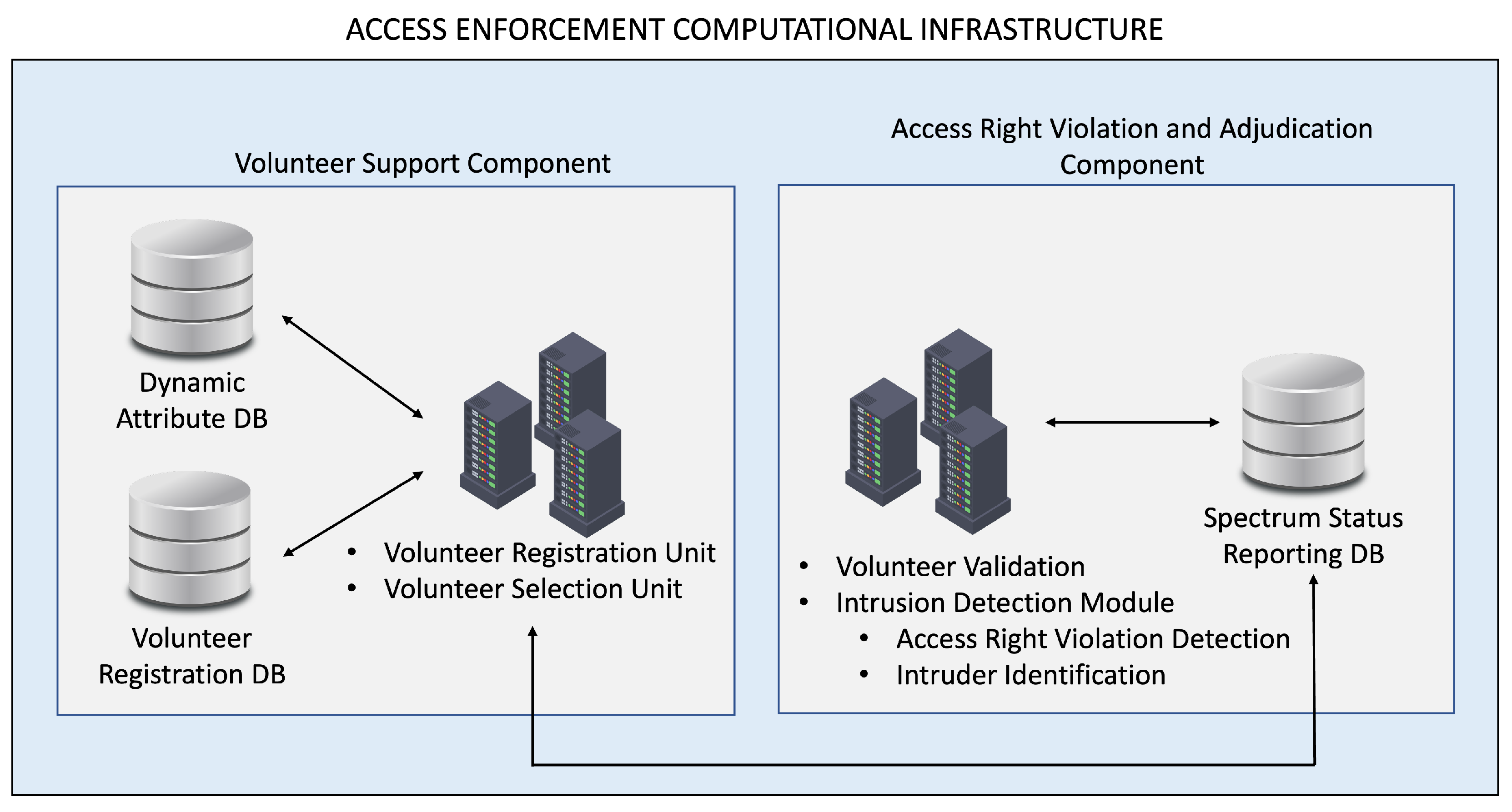
To support these functionalities, the AECI relies on two main components: the Volunteer Support Component and the Adjudication Component. The AECI architecture is illustrated in Figure 2. The detailed features and functionalities of these components are discussed below.

3.1.1. Volunteer Support Component (VSC)

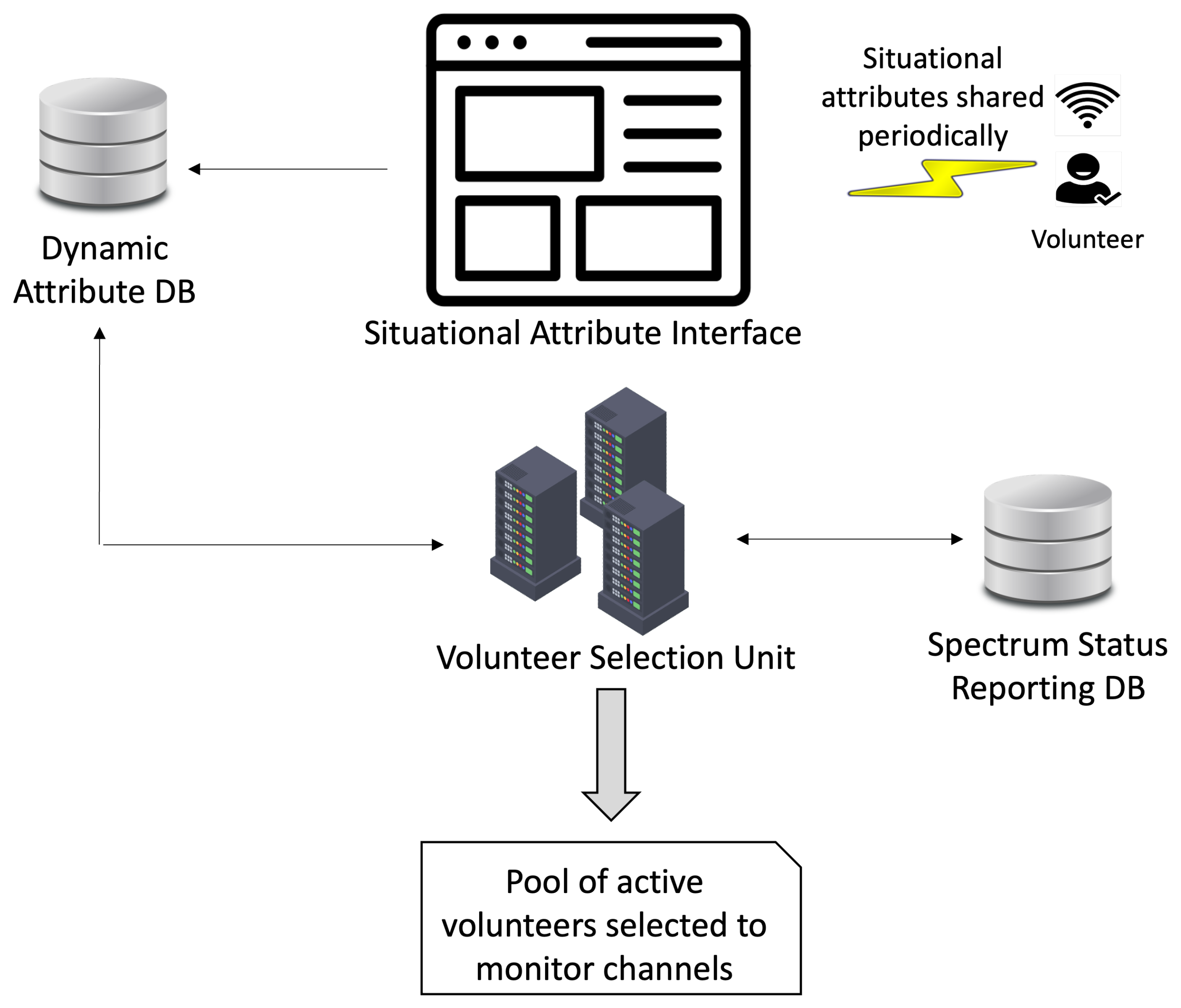
The VSC uses the Volunteer Registration Unit (VRU) to handle volunteer registration. Volunteers submit personal data and information related to their communication device capabilities through the VRU registration interface. The Volunteer Registration Database (VRD) is used to host this information. The VSC also uses the Volunteer Selection Unit (VSU) to handle the selection of volunteers to monitor spectrum. To this end, the VSU uses the Dynamic Attribute Database (DAD) to host information related to volunteers’ location and mobility management. This information is needed during the selection process to estimate volunteers’ locations, as they move, and the length of their stay in these locations. The database also stores the information required to evaluate volunteers’ spectrum monitoring performance. The VSU leverages data from both the VRD and the DAD to support volunteer selection processes.

Volunteer Registration Unit (VRU) 

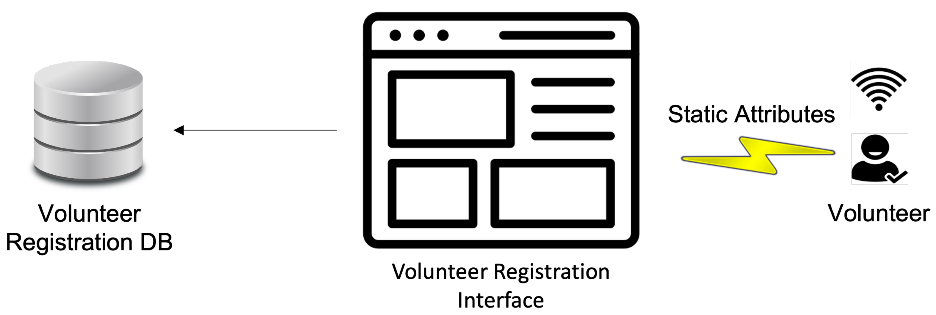
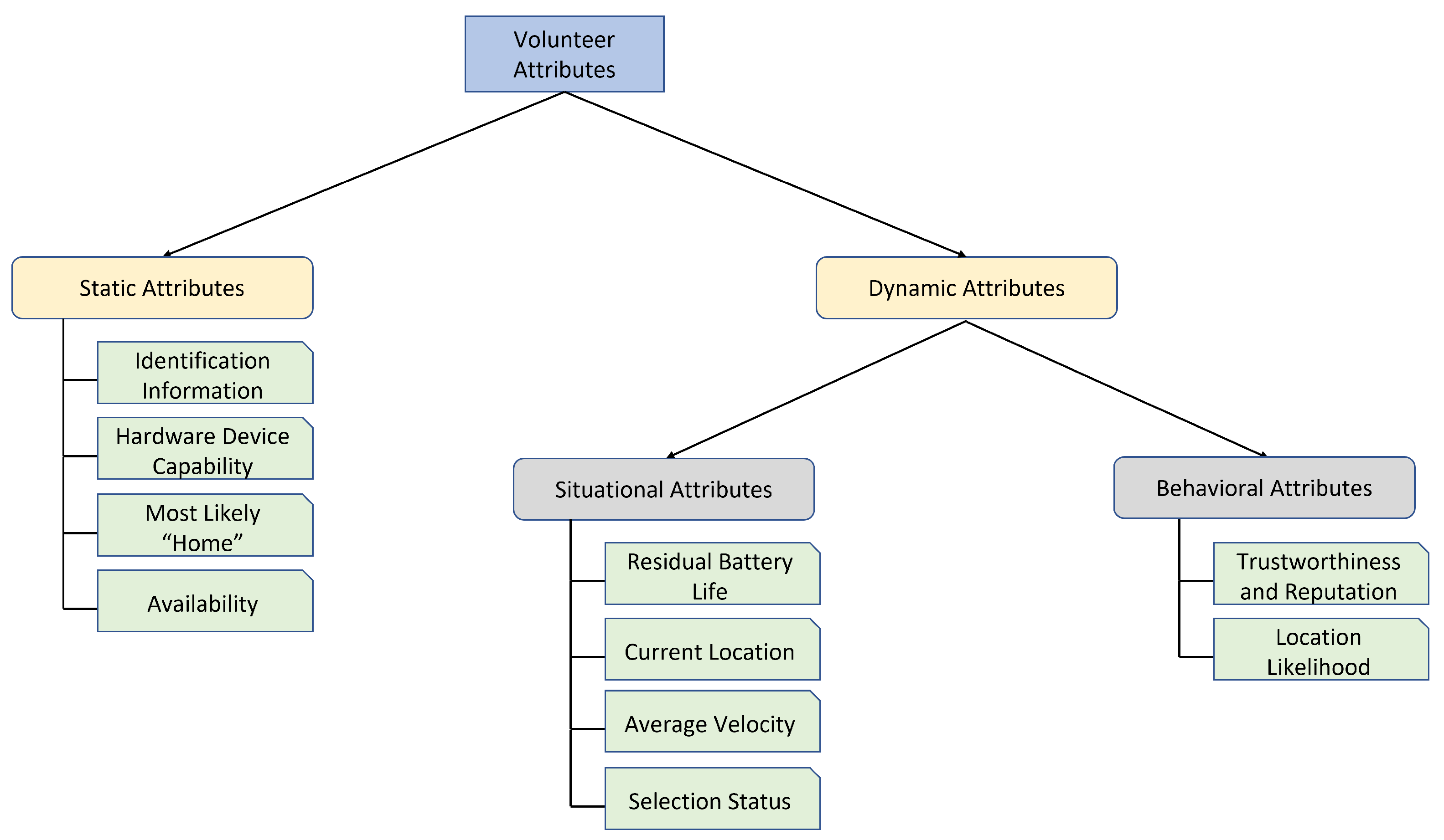
Volunteers must register to be considered for participation in spectrum monitoring. As shown in Figure 3, the registration is completed through the VRU interface of the SCS Access Enforcement Computational Infrastructure. The information provided by volunteers includes both static and dynamic attributes. Static attributes represent information that is common to all volunteers, including personal identification information, contact details, ‘most-likely domicile’, scheduling availability, in terms of daily time slots during which monitoring activities can be performed, and communication device characteristics and capabilities. These attributes are essential in guiding the selection process, ensuring decisions are based on criteria relevant to the spectrum monitoring activity.

Dynamic attributes characterize volunteers’ involvement and impact on the spectrum monitoring activity over time. They are used to achieve real-time, efficient task assignment by capturing current availability, monitoring accuracy and engagement levels during a monitoring interval, ensuring optimal matching between spectrum coverage areas and volunteers, based on current and changing conditions [8].

These attributes are updated during each monitoring interval. They are used, at the end of a monitoring interval, to guide decisions about assigning volunteers to communication channels within a spectrum coverage area. Dynamic attributes can be situational or behavioral. Situational attributes include current geographical location, average velocity, residual battery life of the sensing device, measured in terms of remaining useful life, and selection status. The situational attributes are used to estimate the likelihood of a volunteer to reside within a spectrum monitoring area, over a specific time period. Behavioral attributes are assessed based on volunteers’ spectrum monitoring performance. They include trustworthiness, reputation, and location likelihood, which represents the likelihood of a person residing in a specific location within the monitoring region. These dynamic attributes are stored in the DAD. The details of static and dynamic attributes are depicted in Figure 4.

Volunteer Selection Unit (VSU) 

The main objective of the VSU is to select volunteers to monitor spectrum within a geographical access right enforcement area. An effective volunteer selection procedure should ensure the following:

• High accuracy in detecting enforceable events, including access right violation and spectrum interference;
• Adaptability to changes in the access right enforcement policies and environment;
• ‘Optimum’ alignment of volunteers’ monitoring capabilities and personal preferences with the spectrum monitoring activity objectives.

To meet the above requirements, the proposed framework uses an algorithm that considers volunteers’ attributes and spectrum monitoring objectives, when making selections. The algorithm combines the advantages of the multiple-choice secretary algorithm with a variant of the stable matching algorithm to ensure close alignment of volunteers’ attributes and preferences with the objectives of the spectrum monitoring activity. Details of this algorithm are provided in [7].

Upon volunteer selection, a procedure is established to assign channels to volunteers within an access right enforcement area, where they are most likely to reside. As shown in Figure 5, the VSU utilizes the information in the VRD and the DAD to make decisions related to volunteer selection and channel assignment. Volunteers’ situational attributes are used in real time to estimate their likelihood of being present in a specific geographical region during a spectrum monitoring interval. These attributes are also used to evaluate their effectiveness in monitoring channels. The outcome of this evaluation is used to update the volunteers’ trustworthiness and reputation, over each monitoring interval. Repeated inaccurate reporting on channel status reduces volunteer’s trustworthiness and negatively affects reputation. If a volunteer’s reputation score drops below the threshold, they are replaced by a standby volunteer prior to the next monitoring interval.

3.1.2. Access Right Violation and Adjudication (ARVA)

The primary tasks of the ARVA component are to:

• support and validate volunteers’ reporting on spectrum status;
• provide mechanisms to detect unauthorized and intrusive spectrum use, thereby preventing performance degradation for authorized users; and
• enable the identification of spectrum access violators for adjudication.

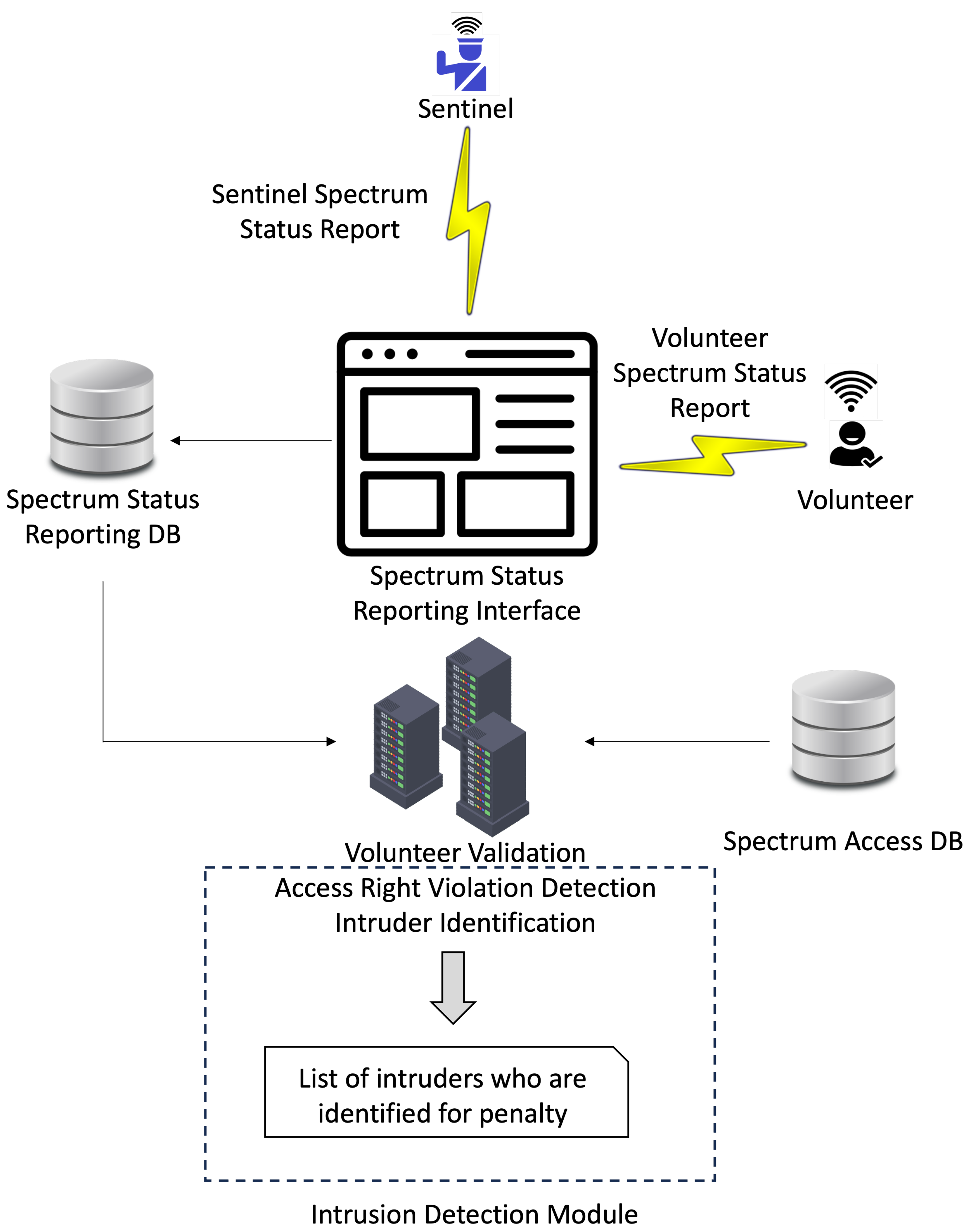
The ARVA tasks are supported by the Spectrum Status Reporting Database (SSR_DB). This database records all reports submitted by volunteers and sentinels over a monitoring interval. In the following, the basic functionalities of the ARVA tasks are discussed.

Volunteer Reporting Validation 

To ensure accurate reporting validation, the access right enforcement activity is performed over adjacent time intervals, referred to as Monitoring Intervals (MIs). Each MI is further divided into time subintervals, referred to as Working Unit Intervals (WUIs). A WUI is defined as the smallest number of transmission slots over which a user can accomplish useful work. Volunteers senses the communication channel over each transmission slot of a WUI and report to the SSR_DB any abnormal conditions, caused by high noise rise or degraded performance, that suggest interference. Sentinels, on the other hand, randomly select WUIs for sensing and report potential interference to the SSR_DB, when abnormal conditions are detected. The volunteer validation unit cross-references the volunteer’s reported channel condition with the sentinel’s corresponding report to identify any discrepancies. The cross-referencing outcome is used to update the volunteer’s reputation. The reputation update mechanism uses a linear function to reward truthful reporting and an exponentially decreasing function to penalize fraudulent reporting. If at the end of a monitoring interval, the reputation of a volunteer decreases below a threshold, the volunteer is expelled [5].

Access Rights Violation Detection 

Volunteers are expected to be equipped with devices capable of detecting end users’ anomalous behavior, including:

• Emulating activities of an incumbent higher priority user by mimicking their signal characteristics, making other currently active lower priority users believe that the incumbent’s channel is occupied. In conformance with spectrum access rules, these users vacate the channel, thereby granting exclusive access of the channel to the fraudulent user.
• Reporting fraudulent channel occupancy or marking a busy channel as idle, which may cause interference with incumbents.
• Exceeding the prescribed transmission power to achieve higher coverage.
• Engaging in transmission over a channel assigned to a different end user.

These capabilities are typically provided by Software-Defined Radios (SDRs), as they provide access to raw in-phase and quadrature (I/Q) data. Such access enables physical-layer fingerprinting. Furthermore, because an SDR typically possesses unique hardware-level impairments, such as I/Q imbalance, DC offset, and phase noise, monitoring systems can identify the specific “RF signature” of a transmitter [49]. By training deep learning models on these signatures, an SDR-based system can distinguish between a genuine military radar and a spoofed PUE signal with high precision, even if the signal profiles appear identical in the time domain [50]. Additionally, SDRs can be used to convert signal captures into spectrograms, which are then processed to identify and classify overlapping signals in real time [51]. Therefore, SDRs can provide the basis for the development of an effective access right enforcement scheme.

Numerous works have been proposed to detect misbehavior in shared-spectrum networks. Liu et al. [22] investigate the problem of detecting unauthorized spectrum usage in DSA networks. The detection of anomalous spectrum usage is formulated by using statistical significance testing. The authors propose two detection schemes based on the mobility of the authorized transmitter. The first scheme is based on the assumption that the Received Signal Strength (RSS) from a single transmitter decays approximately linearly with the logarithmic distance from the source, but this is no longer the case when the RSS is a sum of multiple transmitters at different locations. This scheme is used when the authorized user is mobile. The second scheme is based on the assumption that the transmitters at different locations will lead to different spatial distributions of the RSS and is used when the authorized transmitter is static. However, the authors assume that the unauthorized transmitters are non-colluding and that the authorized transmitters are always trustworthy.

Access Right Violation Adjudication 

When a potentially enforceable event occurs, forensic analysis must be conducted to determine whether a claim can be adjudicated and to build a foundation of evidence for the adjudication process. Thus, one of the overarching objectives of the Access Enforcement Computational Infrastructure is to build a robust information base for adjudication—enabling timely resolution of events and ensuring that costs are appropriately internalized to the responsible actors. As reported in Anderson et al., “spectrum forensic systems are designed to isolate an interference source, to provide evidence of interference and to do so rapidly, inexpensively and without burdensome complexity” [52]. Therefore, spectrum forensics involves systematically identifying the source, time, and location of radio frequency interference (RFI), along with assessing its impact on communications. The source can be a malfunctioning device, an unauthorized transmitter, a rogue access point or an illegal jamming equipment. The source can also be a service provider, with an improperly configured transmitter. Multiple approaches have been proposed, which leverage real-time spectrum monitoring, multi-sensor geolocation, and advanced signal analysis to detect interference [53].

Volunteers and sentinels are required to systematically report channel interference events to assist with forensic analysis. The reported information include signal characteristics, such as frequency signature and signal strength, and identification of communication protocols and device type. The reported information is hosted in the SSR_DB. It is used to assert the occurrence of unauthorized or illegal use of the spectrum, and identify the intruder when an interference event is reported. The SSR_DB is also used to preserve digital evidence related to an interference event, and when necessary conduct specialized digital forensics analysis. The basic components underlying this process, along with the supporting infrastructure, are illustrated in Figure 6.

When an activity is flagged as a potential illegal use of the spectrum, the SCS employs an Intrusion Detection Module (IDM) to identify and confirm that interference originates from an unauthorized user. The first step in resolving interference is identifying the source transmitter. Based on reported information, several effective approaches can be used to locate and identify the interfering transmitter. In an ideal scenario, a PHY-layer authentication procedure can be used to identify a transmuting device [53]. This procedure enables a receiver to swiftly discern between compliant and rogue transmitters, eliminating the need for unnecessary higher-layer processing. The procedure, however, requires that the communication device include a mechanism for authenticating its waveforms. It must also implement tamper-resistant measures to prevent malicious users from circumventing the authentication process [53]. PHY-layer authentication schemes can be intrinsic or extrinsic. Intrinsic schemes utilize the intrinsic characteristics of the transmitted signal as unique signatures to identify transmitters. These methods primarily include RF fingerprinting and electromagnetic signature identification [54,55,56,57]. However, such schemes are sensitive to environmental factors like interference, and temperature changes, and are not effective in “real-world scenarios” [53]. Extrinsic identification schemes, on the other hand, enable authorized transmitters to embed an authentication signal intrinsically into their message signal (like machine authentication code, digital signatures, spectrum permits [17]), which can then be decoded by the receiver [53]. Such techniques include PHY-layer watermarking [58] and transmitter authentication [59,60]. However, such schemes involve the superposition of the message signal over the authentication signal [58]. As such, the signal-to-noise ratio (SNR) of one signal is compromised by the other [53]. Another drawback of this scheme is that the SNR of the received signal must be high so that the received authentication signal is decoded and demodulated successfully by the receiver [53]. To address these challenges, a scheme referred to as “blind transmitter identification” can be used to uniquely identify (or authenticate) a transmitter under low SNR and high multipath fading conditions. Furthermore, the scheme does not require complete knowledge of the PHY-layer transmission parameters to identify the device [53,61].

To complete the interference resolution, IDM cross-references the SSR_DB reported information related to the interfering device with the Spectrum Access Database. The latter contains information on licensed and unlicensed spectrum usage, including authorized transmitters, along with relevant communication restrictions. A decision to grant, suspend, or terminating transmission rights for the interfering device depends on the regulatory rules and protection requirements of the spectrum coverage area.

3.2. Volunteer Management Strategy

The Volunteer Selection Unit (VSU) primarily handles the selection of volunteers to monitor the spectrum over a Monitoring Interval (MI) [5,6,7,8]. Initially, volunteer selection is solely based on the registration information submitted to the VRD. In subsequent MIs, however, the VSU uses the information in both the VRD and the DAD for the selection of new volunteers and the reassignment of active volunteers, based on their monitoring performance in the previous MI. Poor performance of a deployed volunteer may be caused by environmental factors, such as low signal attenuation or a malfunctioning communication device. It may also be caused by behavioral factors, including colluding with unauthorized users to provide them access to protected spectrum. Consequently, a decision must be made, at the end of each MI, to either reassign or replace active volunteers, based on associated performance data, gathered in the previous MI. Volunteers’ unpredictable mobility, combined with potential volunteer ejection due to inadequate monitoring performance, can create coverage gaps in the monitored area. To mitigate this risk, the following mechanisms are implemented:

3.2.1. Standby Volunteers and Patching

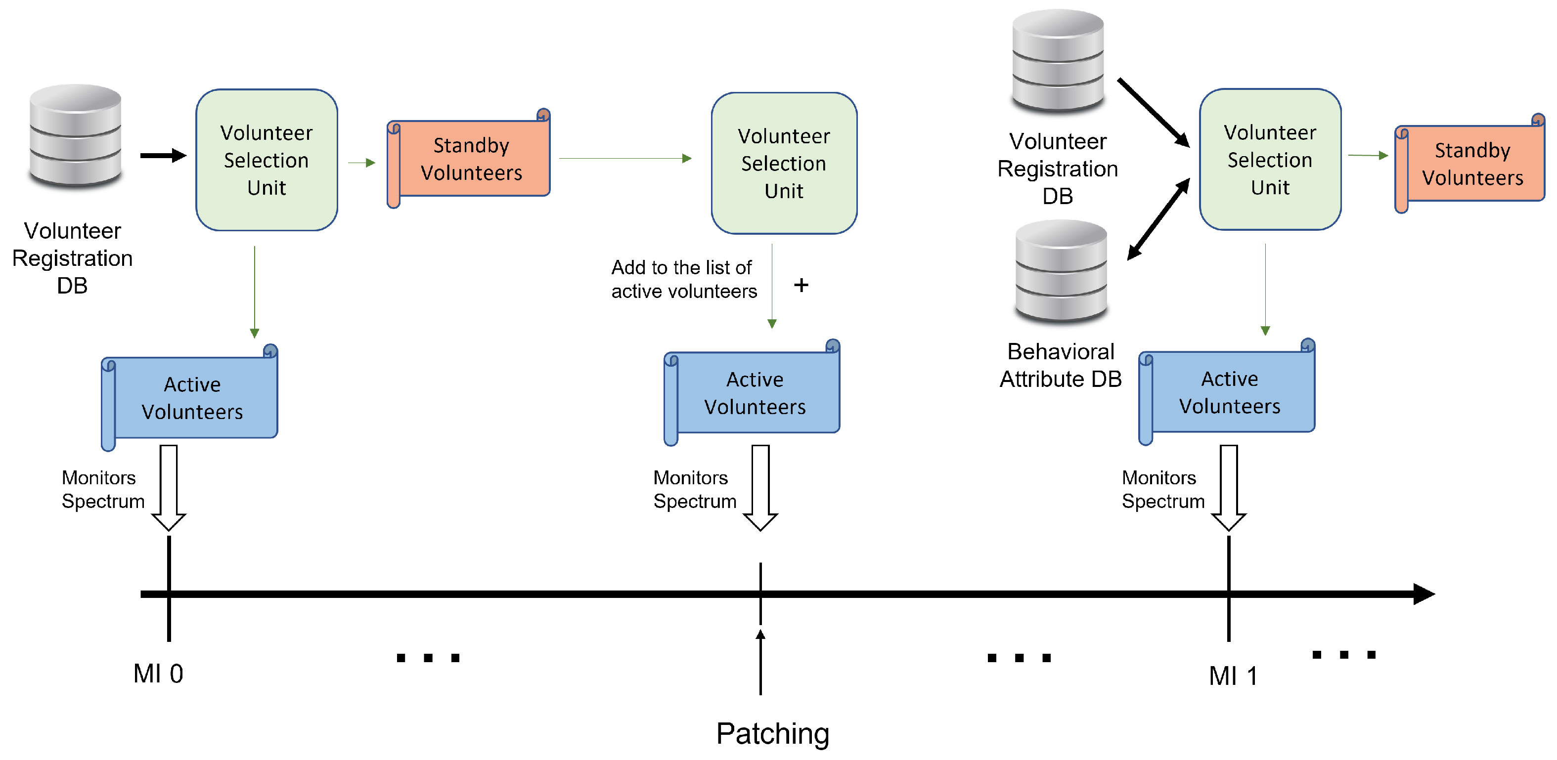
As shown in Figure 7, a number of volunteers may be deemed by the VSU to be qualified to monitor the spectrum. Depending on the targeted region coverage, only a subset of these volunteers, however, is activated to monitor spectrum at the beginning of each MI. These volunteers are referred as active volunteers. The remaining volunteers stay on standby, available as needed, without a fixed schedule, ready to assist with spectrum monitoring if a coverage gap emerges. Standby volunteers play a crucial role in ensuring continuity and resiliency of spectrum monitoring, particularly when volunteers’ mobility is highly unpredictable. Their primary benefit is providing flexible, timely support when active volunteers become unavailable or need to be replaced.

Dynamic patching of the volunteer schedule is used to address coverage gaps, enabling rapid adjustments without disrupting ongoing monitoring operations. This is achieved through the redundancy provided by the standby mechanism. Figure 7 illustrates the volunteer selection and management strategy.

3.2.2. Volunteer Incentives

Incentives play a critical role in recruiting and motivating individuals to participate, stay engaged, and contribute to planned activities over time. Numerous studies have focused on designing and analyzing meaningful and appropriate incentives to gain a better understanding of their effectiveness to motivate and significantly boost a volunteer’s engagement in the planned tasks [62,63,64]. The literature identifies a broad spectrum of incentives used to motivate volunteering, categorized primarily into intrinsic, extrinsic, and intangible motivators.

In essence, intrinsic incentives are internal drivers tied to personal fulfillment. Their likelihood to engage volunteers stems from internal motivations, often derived from the activity itself, such as altruism, personal growth, a sense of purpose, and a sense of self-fulfillment. Volunteers driven by intrinsic motivation often seek to contribute to a “cause” they believe in to strengthen their sense of community, while aspiring to develop new skills, when possible. Intrinsic incentives research shows that volunteers with intrinsic motivations, who feel their volunteering work aligns with their values, show deeper emotional investment, sustained long-term commitment, higher quality of service, and great satisfaction. Research also shows that, while intrinsic incentives are highly effective for long-term engagement, they work best when supported by thoughtful volunteer management and a culture of appreciation. If volunteers realize their assigned tasks are meaningless or if they feel their efforts are unappreciated, their intrinsic drive can diminish. Extrinsic incentives are external rewards offered to volunteers to encourage participation and engagement in crowdsourcing activities. Depending on the nature and objectives of the planned activities, these awards range from monetary stipends and paid volunteer time off to bonuses, certificates, badges of honor, and prizes. Studies show that extrinsic incentives may increase volunteers’ participation and significantly boost their engagement, particularly for those individuals who may be deterred by the time or cost of volunteering. Studies also show that, while effective in boosting short-term engagement, financial incentives may not sustain long-term participation. In particular, studies indicates that monetary rewards can undermine and sometimes crowd-out intrinsic motivation, especially in crowdsourced contexts where the planned activities are designed to benefit people and communities [65].

To address these shortcomings, hybrid approaches, which combine intrinsic and extrinsic incentives to provide “material” and “immaterial incentives”, are often used to better adapt to the nature and objectives of the crowdsourced platform, in order to maximize participation and sustained engagement. Typically, these approaches combine multiple incentive types, including financial rewards, social recognition, and gamification, emphasizing the importance of tailoring incentives to user preferences [66,67,68]. Depending on the context, studies show that hybrid approaches have the potential to increase user activity and retention, with potential for optimal results [69].

The proposed framework does not depend on a specific motivator to recruit and engage volunteers. Instead, the proposed approach embeds in its design intrinsic motivators, focusing on: (i) volunteers’ relatedness to the crowdsourced activities, (ii) self-determination and autonomy in making commitments and selecting monitoring tasks, and (iii) opportunity for social impact. By creating an environment that supports self-determined motivation, the framework enables volunteers to feel valued and connected. Furthermore, these motivators foster a sense of ownership and provide powerful drivers for sustained engagement. To achieve these objectives, the following mechanisms are embedded in the proposed framework.

• Episodic Volunteering: In the proposed framework, the basic commitment is for a monitoring epoch, at the end of which volunteers may either continue or terminate their commitment. This mechanism provides flexibility and accessibility, allowing volunteers to contribute from anywhere, at any time, based on their personal availability and professional schedule. It also enables the quick mobilization of individuals, with varied skills and expertise, who may not want to commit to long-term tasks, but are willing to contribute meaningfully to short monitoring activities.
• Convenient Scheduling: This mechanism harnesses the fact that individuals are intrinsically motivated to help, when the commitments of time and energy are low and the benefits to the community are significant. The proposed framework allows volunteers to use the crowdsourcing platform to register their capabilities, including preferences to which regions they are willing to monitor. This self-determination based approach empowers volunteers to make commitments that match their skills and availability.
• Reputation: The proposed framework provides a reputation model, designed to track and quantify volunteers behavior and reliable contribution to the monitoring tasks. The model embeds trust as a critical component and uses an evidence-based approach to assess volunteers’ performance, in terms of monitoring accuracy and reliability. The reputation model uses the accuracy of reporting on the status of the spectrum to either enhance or degrade their reputation. When the reporting failure rate exceeds a specified threshold, the volunteer is denied participation in the monitoring activities (the details of how volunteer reputation is managed are provided in [5]).

3.3. Enforcement Area Coverage

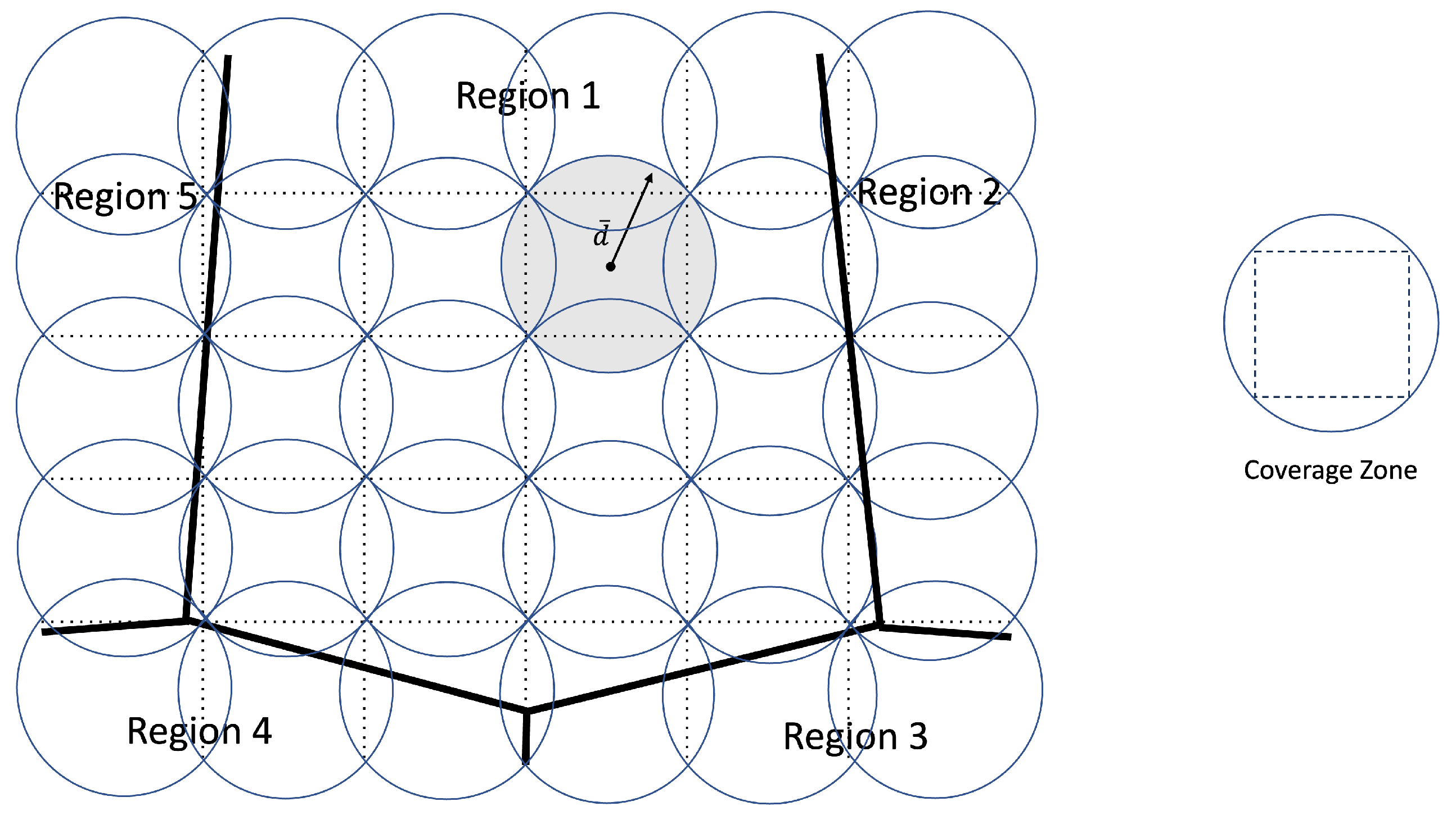
To achieve a balanced coverage, the spectrum access rights enforcement area is partitioned into regions, using adaptive approaches based on Voronoi’s and Lloyd’s algorithm. Details of this algorithm are provided in [7,8]. Furthermore, access policy enforcement within a region can be targeted to be more responsive to local conditions and spectrum access patterns. Achieving comprehensive regional coverage of the enforcement area depends on the volunteer’s device coverage capabilities within a region. It is highly unlikely that a volunteer has the capabilities to cover an entire region during a spectrum monitoring interval. This stems from several factors, including external radio signal interference, limited power of the volunteer’s spectrum sensing device, and physical obstruction. To address these limitations, regions are further subdivided into circular cells, where each cell represents a volunteer’s unit of coverage. The question remains: how to determine the radius of a cell, taking into consideration a combination of factors, including frequency, transmitted power, and antenna type?

Assuming a free space path and isotropic antennas of the spectrum sensing devices, the average distance, $\overline{d}$, before which the received power diminishes below a threshold $\varphi$ is given by (1):

$$\overline{d}=\sqrt{{\displaystyle \frac{\overline{P_t}}{\varphi }}·\left({\displaystyle \frac{c^2}{{\left(4\pi f\right)}^2}}\right)}$$

(1)

In (1), $\overline{P_t}$ represents the average transmitted power of the spectrum sensing device for all volunteers, $\varphi$ denotes the specified threshold power level, c stands for the speed of light in vacuum, and f represents the frequency of the transmitted signal.

Based on $\overline{d}$, a region can be divided into square-shaped zones, where a given zone represents the area of the circumscribed square of the associated circle. Figure 8 shows the partitioning of a given region of enforcement, r, into coverage zones. Let $d_v=\sqrt{{\displaystyle \frac{P_t^v}{\varphi }}·\left({\displaystyle \frac{c^2}{{\left(4\pi f^v\right)}^2}}\right)}$ be the radius of the zone associated with volunteer, v. Considering that the antennas are isotropic, the average area of coverage, A, of a spectrum sensing device can be given by (2):

$$A=\pi ·{\left(\overline{d}\right)}^2$$

(2)

Based on (2), a side of a coverage zone is of length $\sqrt{2}.\overline{d}$, and its area is $2.{\overline{d}}^2$. Therefore, the number of coverage zones, Z, in an enforcement region, r, of surface area $\mathcal{R}$ is be given by (3):

$$Z=\lceil {\displaystyle \frac{\mathcal{R}}{2.{\left(\overline{d}\right)}^2}}\rceil$$

(3)

To this end, it is necessary to select eligible volunteers for monitoring the spectrum in a coverage zone.

As stated above, volunteers are likely to move frequently and unexpectedly from one zone to another. Consequently, associating a single volunteer to cover a given zone is prone to frequent monitoring disruption, thereby presenting a significant threat to long-term sustainability, with far-reaching impacts on spectrum access rights. To address this shortcoming, the proposed framework associates, when possible, more than one volunteer to monitor a zone. In the following, the minimum number of volunteers to ensure a high likelihood of zone coverage, referred to as minimum zone coverage, is derived.

3.4. Minimum Zone Coverage

Given a coverage zone z, let $V_z=\{v_{i}1\le i\le K_z\}$ be the set of eligible volunteers to cover zone z. A volunteer, $v_i$ is eligible to cover zone z if and only if:

• Volunteer, $v_i$, is present in z;
• The coverage radius, $d_i$, provided by $v_i$, is greater than or equal to $\overline{d}$.

Note that the area of a zone, z, covered by a volunteer, v, is $A_z\left(v\right)=\pi ·{\left(d_v\right)}^2$. Depending on where v is currently located within z, $A_z\left(v\right)$ may be less than the expected coverage area, $A=\pi .{\left(\overline{d}\right)}^2$, derived based on (1). The worst-case scenario occurs when the volunteer reaches a corner of the zone, z. Therefore, $d_v$ must be equal to $2.\overline{d}$ to ensure full coverage of z regardless of where v is located within z. It should be noted that this occurs with probability $C_v^z$, as defined in (4):

$$C_v^z=Pr(d_v\ge 2.\overline{d})$$

(4)

In addition to the geographical coverage that can be provided by a volunteer, it is necessary to estimate the likelihood of a volunteer being present in a coverage zone, z. The proposed framework explores the use of three deep learning-based models to predict such a likelihood. More specifically, given a set of volunteers, $V_z=\{v_1,v_2,\dots ,v_K\}$, the models use the location behavior of a volunteer, $v_i$$(1\le i\le K)$$\in V_z$, to predict the zone where $v_i$ is most likely to land at a given time, t. The specific detail of the approach used by these models to predict the landing zone of a volunteer is provided in Section 4.

Given the predicted landing zone of a given volunteer, $v_i(1\le i\le K)\in V_z$, the probability, ${\rho }_{v_i}^z$, that $v_i$ lands in zone z at time t is defined as the accuracy of v’s zone prediction by the underlying model. Notice that $C_v^z$ and ${\rho }_v^z$, when combined, provide an effective quantifiable measure to assess the quality of v’s monitoring, if they were to be selected to cover zone z. In this framework, we use the product, $\Omega ={\rho }_v^z·C_v^z$, for this purpose.

Let $V_z=\{v_i({\rho }_v^z,C_v^z){\rho }_v^z\ge {\alpha }_z\&C_v^z\ge {\beta }_z\}$ be the set of volunteers eligible to cover zone z. Selecting all the volunteers in set $V_z$ will ensure “optimal” coverage of the area of spectrum enforcement. However, there is a tradeoff primarily because selecting a large number of volunteers is expensive as managing a large pool of volunteers can incur excess administrative costs in tasks such as communication and coordination with the volunteers. Therefore, the objective is to minimize the number of volunteers selected from $V_z$ to cover zone z while ensuring that the expected coverage provided by the volunteers is greater than or equal to the threshold, $\Theta$.

Given $\Omega$, and $V_z$, the minimum number of volunteers to cover a given zone, z, is defined as the minimum number of volunteers in $V_z$ that satisfy (5):

$$\sum _{v\in V_z}{\rho }_v^z·C_v^z\ge \Theta$$

(5)

Let $\widehat{V_z}$ be the set of the minimum number of volunteers selected out of $V_z$ to ensure that the coverage provided by the volunteers in zone z is at least $\Theta$ and that the value provided by each volunteer, v, to zone z is ${\mu }_v^z={\rho }_v^z·C_v^z$. Therefore, the minimum number of volunteers, $\widehat{V_z}$, that ensure net value, ${\sum }_{v\in \widehat{V_z}}{\mu }_v^z\ge \Theta$, needs to be determined. In practice, in order to guarantee zone coverage, it is recommended that $\Theta$ be set to 0.9 of the size of $V_z$. It is to be noted that this parameter can be adjusted to closely reflect the monitoring objective of the underlying access rights enforcement policy. In the optimal solution to selecting volunteers for ensuring a net value of at least $\Theta$, there must be a first volunteer, $v_i$, such that its value, ${\mu }_{v_i}^z\le \Theta$. Let the minimum number of volunteers selected, $\widehat{V_z}$, be represented by $T_z[\Theta ]$, which represents the minimum number of volunteers whose total value is $\Theta$. Hence, if ${\mu }_{v_i}^z$ is the value provided by the first volunteer, $v_i$, to zone z in the optimal solution to get a total value of $\Theta$, then $T_z[\Theta ]=1+T_z[\Theta -{\mu }_{v_i}^z]$, i.e., value ${\mu }_{v_i}^z$ is added to $T_z[\Theta -{\mu }_{v_i}^z]$ to optimally get the value of $\Theta$. It is not known who is the first volunteer, $v_i$, that gives the optimal solution but it can be determined by checking the value provided by all the volunteers in $\widehat{V_z}$, and the value of the optimal solution must correspond to the minimum value of $1+T_z[\Theta -{\mu }_{v_i}^z]$ by definition. Moreover, if $\Theta =0$, then the number of volunteers required is 0, as shown in (6).

$$T^z[\Theta ]=\left\{\begin{array}{cc}0\hfill & \mathrm{if}\Theta =0\hfill \\ \underset{i:{\mu }_{v_i\le \Theta }}{min}\{1+T[\Theta -{\mu }_{v_i}]\}\hfill & \mathrm{if}\Theta >0\hfill \end{array}\right.$$

(6)

Algorithm 1 gives a bottom-up solution to determine the minimum number of volunteers in set $V_z$ that can provide expected coverage of the value $\Theta$ to zone z.

Algorithm 1 Minimum number of volunteers in zone z($V_z$, $\Theta$)

1: Input: List $V_z$ of volunteers in zone z, constant $\Theta$ as threshold 2: Output: List ${\mathcal{V}}_z$ of volunteers selected for zone z 3: Initialize array $T_z$ of size $\Theta +1$ with all elements set to ∞ 4: ${\mathcal{V}}_z=\varnothing$ 5: $T_z\left[0\right]\leftarrow 0$ 6: for $p\leftarrow 0$ to $\Theta$ do 7:    min $\leftarrow \infty$ 8:    for $i\leftarrow 1$ to $V_z$ do 9:      if ${\mu }_{v_i}^z\le p$ then 10:         if $1+T_z[p-{\mu }_{v_i}^z]<\min$ then 11:           min $\leftarrow 1+T_z[p-{\mu }_{v_i}^z]$ 12:           ${\mathcal{V}}_z\leftarrow {\mathcal{V}}_z$$\cup v_i$ 13:         end if 14:      end if 15:    end for 16:    $T_z\left[p\right]\leftarrow \min$ 17: end for 18: return ${\mathcal{V}}_z$

The above algorithm recursively builds the list of volunteers, ${\mathcal{V}}_z$, composed of the minimum number of volunteers, $T_z[\Theta ]$, required to ensure the specified level of coverage threshold, $\Theta$. Therefore, the target number of volunteers to be selected, $V_T$, in a geographical area of spectrum enforcement is the sum of the minimum number of volunteers in zone z to achieve expected coverage over $\Theta$ across all zones in every region, r, of the enforcement area, R, as shown in (7):

$$V_T=\sum _{r\in R}\sum _z{T}_z^r[\Theta ]$$

(7)

Volunteers who are selected to monitor the spectrum over a geographical area may not always be honest in reporting the spectrum access events. Corrupt volunteers present the risk of disturbing the spectrum monitoring process by reporting falsely on the spectrum access. To overcome the expulsion of corrupt volunteers upon detection, it is necessary to select the number of volunteers such that the overall corruption is mitigated.

In addition to satisfying the geographical constraints, the target number of volunteers to be selected, $V_T\left(z\right)$, must take into consideration the likelihood of the presence of corrupt volunteers in the pool of selected volunteers, $V_z$. Assuming that in a given zone, z, the probability of a volunteer being corrupted, $P_C$, is uniform, the probability that the number of corrupt volunteers, $V_T^C\left(z\right)$, among a total number of volunteers, $V_T\left(z\right)$, is equal to k, can be expressed in (8):

$$Pr(V_T^C\left(z\right)=k)=\left({\displaystyle \genfrac{}{}{0pt}{}{V_T\left(z\right)}{k}}\right)P_C^k{(1-P_C)}^{V_T\left(z\right)-k}$$

(8)

The expected number of corrupt volunteers, $\overline{V_T^C}$, of the binomial distribution is given by (9):

$$\overline{V_T^C}\left(z\right)=\sum _{k=1}^{V_T\left(z\right)}\left({\displaystyle \genfrac{}{}{0pt}{}{V_T\left(z\right)}{k}}\right)P_C^k{(1-P_C)}^{V_T\left(z\right)-k}=P_C·V_T\left(z\right)$$

(9)

To mitigate the impact of volunteer corruption, it is necessary to increase the size of the selected volunteers, $V_T\left(z\right)$, by $\overline{V_T^C}\left(z\right)$ standby volunteers from the set of volunteers, $V_z$. The standby volunteers are engaged in the monitoring process any time an active volunteer who has been identified as corrupt is evicted. It is to be noted, however, that the size of the remaining volunteers in $V_z$ may be less than $\overline{V_T^C}\left(z\right)$. Taking this into consideration, the number of standby volunteers, $S_z$, is the minimum of the expected number of corrupt volunteers among $V_T\left(z\right)$ and the remaining number of volunteers in $V_z$, as shown in (10):

$$S_z=minimum(V_z-V_T,\overline{V_T^C})$$

(10)

4. Volunteer Availability Likelihood in a Zone

Predicting the availability of a volunteer to be selected for spectrum monitoring in a zone, z, during a monitoring interval, M, requires the development of a volunteer availability prediction model, which uses various factors, including movement patterns, places of residence and work, and itinerary, to predict future volunteer residence. To this end, we analyzed datasets that contain the location behavior of users in Bejing, that were collected over a 5-year period [70,71,72]. The analysis of these datasets guided the development of the volunteer availability prediction model [8].

In sequential data, the order and arrangement of elements are important. In such data, each element is positioned in a specific sequence, and the relationships or patterns between elements are often crucial for understanding the movement pattern [73]. As such, sequential data can be viewed as a time series, where observations are recorded over time, and sequences of events or symbols can be analyzed using machine learning (ML) approaches typically used to process and predict patterns in natural languages, DNA sequences, and musical compositions. Sequential data helps to address the challenges of predicting volunteer availability likelihood in the following ways:

• Capturing the temporal dynamics of volunteers’ movement, which can be used to enhance volunteer availability prediction;
• Recognizing recurrent volunteer’s movement patterns aids in the prediction of future locations;
• Enabling the personalization of the availability prediction model.

4.1. Location Behavior Analysis for Volunteer Availability Prediction

To capture dependencies, trends, or movement patterns that evolve over the ordered sequence of data points, a deep learning-based algorithm can be used to carry out the analysis of the sequential data and predict the next location based on the previous location. Recurrent Neural Networks (RNNs) are commonly employed in machine learning to handle and extract meaningful information from sequential data. The architecture of RNNs and their variants are designed to capture dependencies in sequential data and make predictions based on historical context. Transformers have also been used to model large-scale tasks, where complex feature interactions are prevalent, and large tasks, where the need to achieve high performance outweighs resource constraints.

In this paper, we focus on two variants of RNNs, namely Long Short-Term Memory (LSTM) networks and Gated Recurrent Units (GRU), and a Transformer-based architecture to model sequential data for predicting future zone availability of volunteers.

• LSTM is a type of Recurrent Neural Network (RNN) designed to learn long-term dependencies in sequential data. Its architecture includes a memory cell and three gating mechanisms—the forget gate, input gate, and output gate—which regulate the flow of information. These gates allow the network to selectively retain, update, or discard information over long time intervals, helping mitigate the vanishing gradient problem in standard RNNs.
• GRU is another RNN architecture for sequential data. Like LSTM, it uses gating mechanisms to control information flow. However, a GRU has two gates: the update gate, which controls how much past information is carried forward, and the reset gate, which controls how much past information is ignored when computing the new state. Unlike LSTM, GRU does not maintain a separate memory cell as it combines memory and hidden state.
• The Transformer architecture relies on self-attention mechanisms to model dependencies between all positions in a sequence. This enables the processing of entire sequences in parallel and removes the need for recurrence, allowing better scalability and long-range dependency modeling.

Table 1. Comparison of LSTM, GRU, and Transformer architectures.

Model	Type	Key Properties
LSTM [75]	RNN-based	Processes data sequentially; uses three gates (input, forget, output); maintains a memory cell for long-term dependencies
GRU [74]	RNN-based	Processes data sequentially; uses two gates (update, reset); simpler architecture than LSTM; typically faster training
Transformer [76]	Attention-based	Processes sequences in parallel; uses self-attention; employs positional encoding; foundation of models such as BERT and ChatGPT

compares the key properties of the three AI models. Both GRU and LSTM are designed to address the vanishing gradient problem which is prevalent in RNNs and capture long-range dependencies in sequential data  [74]. However, GRUs, having fewer gating mechanisms compared to LSTMs, result in a simpler architecture with fewer parameters to learn [74]. In addition, the recent popularity of Transformers being able to capture long-term dependencies motivates the comparison of a Transformer-based volunteer availability prediction model with the LSTM and GRU-based models. The Transformer differs from RNNs by not processing data sequentially, enhancing parallelization, and shortening training times by utilizing multiple GPU cores.

4.2. Volunteer Selection and Zone Prediction Workflow

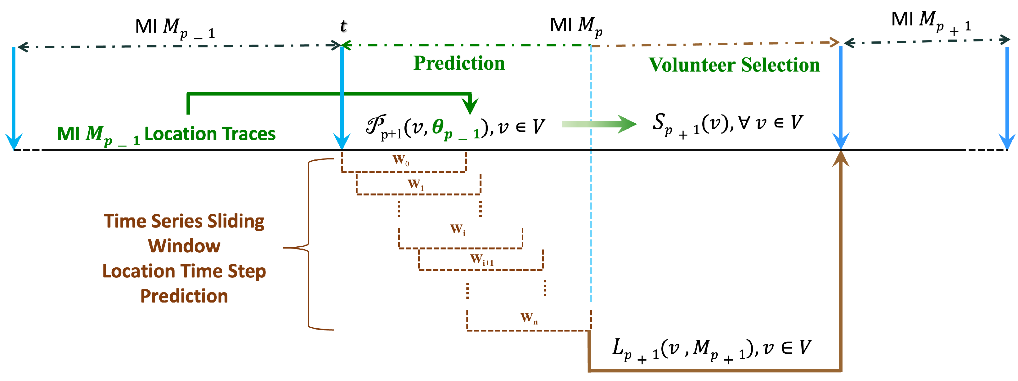
As discussed in [7], volunteers are selected to monitor the spectrum in each spectrum enforcement region by utilizing variants of the Secretary and Stable Matching algorithms at the beginning of every monitoring interval. The zones predicted by the LSTM, GRU, and Transformer models, using the volunteers’ location behavior, are used to select a pool of volunteers that provide sufficient zone coverage. All such volunteer pools are aggregated into a region-level candidate list of volunteers. This candidate list is then fed to the volunteer selection algorithm to select the most qualified volunteers for spectrum monitoring in a region. As shown in Figure 9, in a monitoring interval (MI), $M_p$, the volunteer availability prediction model is used for zone prediction, $P_{p+1}(v,{\theta }_{p-1})$, of a volunteer v over MI, $M_{p+1}$, by learning v’s movement pattern from past location behavior, ${\theta }_{p-1}$, in MI, $M_{p-1}$. The LSTM, GRU, and Transformer-based prediction models utilize the sliding windows $w_0,w_1,w_2,\dots ,w_n$ to learn the temporal dynamics of the movement pattern of v and predict the location of v at a future timestamp. The window, $w_n$, is used to predict the location, $L_{p+1}(v,M_{p+1})$, of v at the start of MI, $M_{p+1}$. The predicted zone using $P_{p+1}(v,{\theta }_{p-1})$ is used for volunteer selection and region assignment over the MI, $M_{p+1}$.

Algorithm 2 summarizes the volunteer zone prediction and selection workflow for each monitoring interval, $M_p$. Firstly, the trained AI-based volunteer coverage zone predictor, $\mathcal{M}$ (LSTM/GRU/Transformer), estimates each volunteer’s next zone, z. Next, we compute a qualification score ${\Omega }_v^z$ for v from their predicted zone availability likelihood, ${\rho }_v^z$, and coverage capability, $C_v^z$. For each zone, z, an eligible pool of volunteers, $V_z$, is formed and the minimum number of required volunteers is computed as $T_z[\Theta ]=\mathrm{Algorithm}$ 1 $\left(V_z,k,\Theta \right)$. We then invoke Algorithm 1 to compute the required list of the minimum number of volunteers, ${\mathcal{V}}_z$, to ensure at least a specified level of coverage threshold, $\Theta$, in z. Finally, every zone-level set, ${\mathcal{V}}_z$, in $z\in Z$ is aggregated by enforcement region and processed by the volunteer selection algorithm for region-level assignment [7]. The final selection of volunteers would depend not only on predicted zone level coverage but also on other attributes like trustworthiness, reputation, and volunteer preferences.

Algorithm 2 Volunteer Selection and Zone Prediction Workflow

1: Inputs: Location traces for each volunteer $v\in V$; monitoring interval $M_p$; window length w; prediction horizon n; set of coverage zones, Z; thresholds $({\alpha }_z,{\beta }_z,\Theta )$; trained AI-based volunteer coverage zone predictor, $\mathcal{M}$. 2: Preprocess traces: clean and time-order location traces for each v; form sliding windows $w_0,\dots ,w_n$ of length w. 3: for each monitoring interval $M_p$ do 4:    for each volunteer $v\in V$ do 5:      Predict v’s GPS coordinate $L_{p+1}(v,M_{p+1})$ using $\mathcal{M}$ and the most recent window $w_n$. 6:      Map $L_{p+1}(v,M_{p+1})$ to a the corresponding coverage zone z. 7:      Update the probability, $p_v$, that v lands in z as the accuracy of v’s zone prediction by $\mathcal{M}$ 8:      Update the coverage, $C_v^z$, provided by v 9:      Compute v’s qualification score, ${\Omega }_v^z\leftarrow {\rho }_v^z·C_v^z$. 10:    end for 11:    for each zone $z\in Z$ do 12:      Build eligible pool of volunteers, $V_z=\{v({\rho }_v^z,C_v^z){\rho }_v^z\ge {\alpha }_z\&C_v^z\ge {\beta }_z\}$. 13:      Compute the required list, ${\mathcal{V}}_z=\mathrm{Algorithm}1\left(V_z,\Theta \right)$, of minimum number of volunteers to ensure the specified level of coverage threshold, $\Theta$, in z. 14:      Aggregate the zone-level list of selected volunteers, ${\mathcal{V}}_z$, into a region-level candidate list of active volunteers and apply the Volunteer Selection algorithm, $S_{p+1}\left(v\right)$ [7] to select and assign volunteers for each enforcement region (a region consists of multiple coverage zones). 15:    end for 16: end for

5. Experimental Setup

To gain a better understanding of the performance and benefits of each algorithm, the LSTM, GRU, and Transformer models are evaluated, using real-world location traces of mobile users. In the following sub-sections, the dataset and data preprocessing techniques, along with experiment methodology and the metrics, used in this experiment are discussed. Following this, the methodology used to carry out the comparative analysis is presented [8].

5.1. Dataset and Data Preprocessing

The volunteer availability prediction models are assessed using the Geolife dataset which is a collection of GPS trajectories [70,71,72]. This dataset was gathered by Microsoft Research Asia over five years (from April 2007 to August 2012) from 182 users as part of the Geolife project. It consists of timestamped points with latitude, longitude, and altitude information. The dataset comprises 17,621 trajectories covering a total distance of 1,292,951 km and a total duration of 50,176 h. These trajectories were recorded by various GPS loggers and GPS-enabled phones, with different sampling rates. Approximately $91.5\%$ of the trajectories are densely represented, with points logged every 1–5 s or every 5–10 m [70,71,72]. The dataset captures diverse outdoor movements, encompassing daily routines like commuting to work or going home, as well as recreational activities such as shopping, sightseeing, dining, hiking, and cycling.

We select Geolife for three primary reasons. Firstly, our goal is to model the mobility pattern that would be expected from potential volunteers who carry GPS-enabled devices and participate opportunistically in monitoring while performing everyday activities; Geolife contains long-term location traces with heterogeneous activities and sampling rates, which is suitable for learning such temporal mobility patterns. Secondly, the dataset provides sufficient trajectory length and density to train sequence models (LSTM/GRU/Transformer) without heavy interpolation, thereby reducing bias introduced by imputation. Finally, the dataset is widely used and well documented, which facilitates reproducibility and comparison across models and parameter settings.

Regarding generalizability, the mobility statistics in Geolife reflect the Beijing-centered user population and may differ from volunteers in other regions of the world. However, the modeling objective in this paper is not to claim that Beijing trajectories are universally representative; rather, it is to utilize data specific to volunteers’ location traces at different times to predict their availability and ability to achieve coverage reliably in a specific zone. The same pipeline (data preprocessing, windowing, training, and evaluation) can be applied to region-specific mobility datasets (e.g., other cities/countries and different transportation cultures) to calibrate model parameters and quantify performance under local behavior. Therefore, the Geolife dataset serves as a realistic benchmark for validating the approach, while deployment in a new region would require retraining using local volunteer traces to account for differences in travel behavior, geography, and device usage.

Prior to carrying out the analysis, the dataset is preprocessed to completely remove corrupt or inaccurate records. The data is also checked for consistency and uniformity. The following steps are used to achieve these tasks and ensure the dataset suitability for analysis:

• All the rows with null or void columns are dropped.
• Since RNN and Transformer models are usually proficient in learning long-term dependencies in large datasets, these models are trained and tested with the data of volunteers that have at least 5000 timestamped data points.
• Since the majority of data points originate in Beijing, China, only the location of volunteers over Beijing, specifically in the area bounded by latitudes 39.6 and 40.2 and longitudes 116.0 and 116.8, are predicted. To this end, only the data points that are within this geographical area are utilized.

In this work, the models are trained using only the ordered timestamped GPS trajectories of each user. No additional exogenous variables (e.g., weather, points of interest, transportation mode labels, map-matching constraints, or calendar/event information) are incorporated. This allows the evaluation to focus on what can be learned from mobility traces alone and avoids assuming the availability of additional information that may not be consistently accessible (or may raise privacy concerns) in practical volunteer deployments. Incorporating such variables, when available, is left for future work.

The following discusses the experimental methodology to perform a comparative performance analysis of the models.

5.2. Methodology

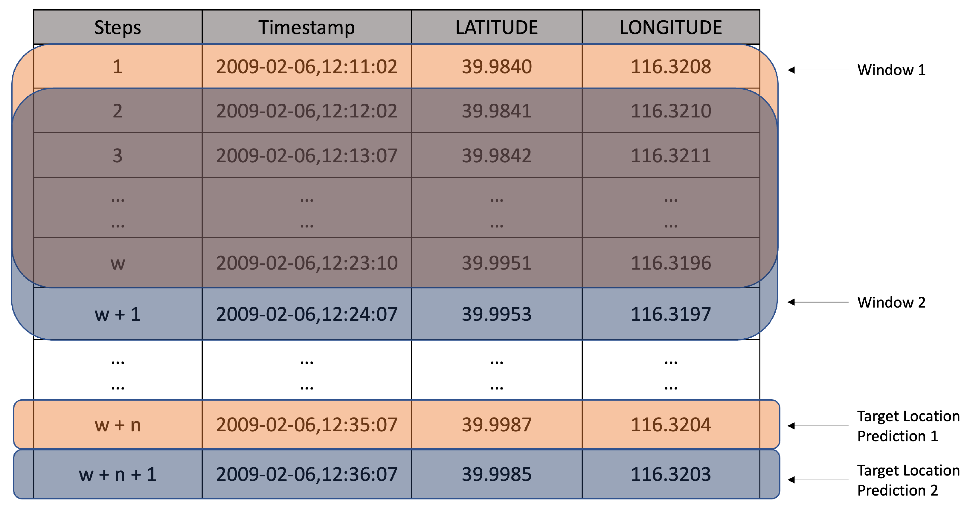
The LSTM, GRU, and Transformer models are trained by using a sliding window technique, such that a series of overlapping sequences or windows is created from the original sequential data. As shown in Figure 10, the sequential data of latitudes and longitudes is divided into fixed-size windows. Each window of size w contains a number of consecutive location time steps. There is a corresponding target location, which is predicted based on w over n steps in the future. In order to capture the continuous patterns and dependencies in the sequential data, the windows overlap. This means that each time step is part of multiple windows. For example, with a window of size w, the window starting at time step i would be $i,i+1,i+2,\dots ,i+w$ and the target location to estimate would be in time step $i+w+n$. Similarly, the next window would be $i+1,i+2,i+3,\dots ,i+w+1$ and the target location to estimate would be in time step $i+w+n+1$. These overlapping windows are used to train the prediction models using a supervised learning approach. The input sequences are fed into the network, and the model is adjusted to minimize the difference between its predictions and the actual target outputs. This training process using sliding windows enables the prediction models to learn and capture temporal patterns, dependencies, and trends present in the time-series location traces. After training, the volunteer availability prediction models can be used to make predictions on new, unseen data by sliding the window similarly.

5.3. Performance Metrics

The following metrics are used for evaluating the performance of the volunteer location prediction approaches.

• Accuracy: As discussed in Section 3, effective spectrum monitoring is ensured by dividing the geographical area into smaller regions. For this experiment, the geographical area is divided into 49 equal-sized square regions. The latitude and longitude values that are predicted by the deep learning models for a volunteer are mapped to one of these regions. To determine the accuracy of prediction of the LSTM and GRU models, their predicted region for a volunteer is compared to the actual region in which the volunteer resides at a given time in the future. Assuming that:

  -

  ${\gamma }_v$ is the number of predictions made for a volunteer, v;

  -

  $X_v^i$ is an indicator function such that $X_v^i=1$ if the predicted region is the same as the actual region for the $i^{th}$ location prediction of a volunteer, v, and $X_v^i=0$ otherwise.

  The accuracy, $A_v$, in predicting the future regions of a volunteer, v, is defined as the sum of the indicator functions divided by the total number of predictions.

  $$A_v={\displaystyle \frac{1}{{\gamma }_v}}\sum _{i=1}^{{\gamma }_v}{X}_v^i$$

  (11)
  In other words, accuracy is the ratio of the frequency of correct predictions to the total number of predictions.
• Root Mean Square Error (RMSE): RMSE provides a measure of the average deviation between predicted and actual values of latitude and longitude, with lower RMSE values indicating better predictive accuracy. This is given by (12) as shown below:

  $${\mathrm{RMSE}}_v=\sqrt{{\displaystyle \frac{1}{{\gamma }_v}}\sum _{i=1}^{{\gamma }_v}{(y_v^i-{\widehat{y}}_v^i)}^2}$$

  (12)
  In (12), ${\gamma }_v$ represents the total number of predictions made for a volunteer v, $y_v^i$ represents the observed latitude and longitude values for the $i^{th}$ data point, and ${\widehat{y}}_v^i$ represents the predicted latitude and longitude values for the $i^{th}$ data point.
• Geodesic Distance: The geodesic distance, $d_g^v$, between the predicted location and the actual location of a volunteer, v, is the next performance metric that is used. It is a measure of the shortest path between the predicted and actual location of v. It takes into account the curvature of the sphere and provides a more accurate distance calculation for points specified by latitude and longitude than a simple Euclidean distance. It is often used in geography, navigation, and mapping applications where precise measurements of distances over the Earth’s surface are required [77,78]. A lower geodesic distance between the predicted and actual location of a volunteer indicates better performance of the volunteer mobility model.
• Execution Time: The execution time is a metric that gauges the average duration required to train and test a deep learning model for predicting a volunteer’s future location. A lower execution time indicates a better performance.

5.4. Model Architectures

After the Geolife dataset is cleaned and preprocessed using the steps underlined in Section 5.1, the number of volunteers whose location traces are used to train and test the deep learning models is 116. The experimental dataset was constrained to a geographical bounding box encompassing the Beijing metropolitan area, defined by latitude coordinates $[39.6,40.2]$ and longitude coordinates $[116.0,116.8]$. To facilitate gradient stability and model convergence, raw coordinate pairs were normalized to a $[0,1]$ range via Min–Max scaling based on the training distribution. The data was partitioned chronologically, with the first $70\%$ of observations used for model fitting and the remaining $30\%$ reserved for out-of-sample evaluation. We formulated the trajectory prediction task using a sliding window approach with a look-back window of $N=12$ time steps. The target variable was defined as the coordinate pair at $t+12$ relative to the end of the input sequence, establishing a significant forecasting horizon to test the model’s predictive robustness.

In both the LSTM and GRU-based volunteer mobility models, there are four LSTM and GRU layers, respectively. The first three layers consist of 64 units each and return the entire sequence of outputs, while the fourth layer, with 32 units, only returns the final output in the sequence. The Rectified Linear Unit (ReLU) activation function is used in all the layers to promote non-linearity in the model. The architecture of both the mobility models concludes with a final dense layer featuring two units, indicative of its application to regression tasks aiming to predict the future latitude and longitude values of a volunteer. Parameter optimization was conducted using the Adam algorithm to minimize the Mean Squared Error (MSE) over 10 training epochs.

The Transformer model is designed for time-series regression. Input vectors in ${\mathbb{R}}^2$ are first projected into a 64-dimensional latent space through a linear embedding layer. The Transformer backbone comprises a stack of two encoder layers, each utilizing a multi-head self-attention mechanism with four heads and a position-wise feed-forward network with a hidden dimension of 256. To improve generalization and prevent co-adaptation of features, a dropout probability of $0.2$ was applied within each encoder block. The resulting temporal feature maps are flattened and passed to a final dense layer, which maps the $12\times 64$ internal representation to the final two-dimensional output vector. Model parameters were optimized using the Adam algorithm with a fixed learning rate of $0.001$ over 10 training epochs. We employed Mean Squared Error (MSE) as the objective function to minimize the distance between the predicted and ground-truth normalized coordinates. Training was performed with a batch size of 64 and stochastic shuffling to ensure varied gradient updates. All predicted outputs were subsequently transformed back to their original coordinate scales to allow for the calculation of the required performance metrics.

6. Results and Discussion

For our experiments, the first $70\%$ of the location traces of each volunteer is used for training and the remaining $30\%$ of it is used for testing [8]. While training and testing, the sliding window size of 12 and the 12th location sequence from the end of the window is predicted. During training, the model’s weights are iteratively updated to minimize the specified loss function over several epochs. The training concludes after 10 epochs.

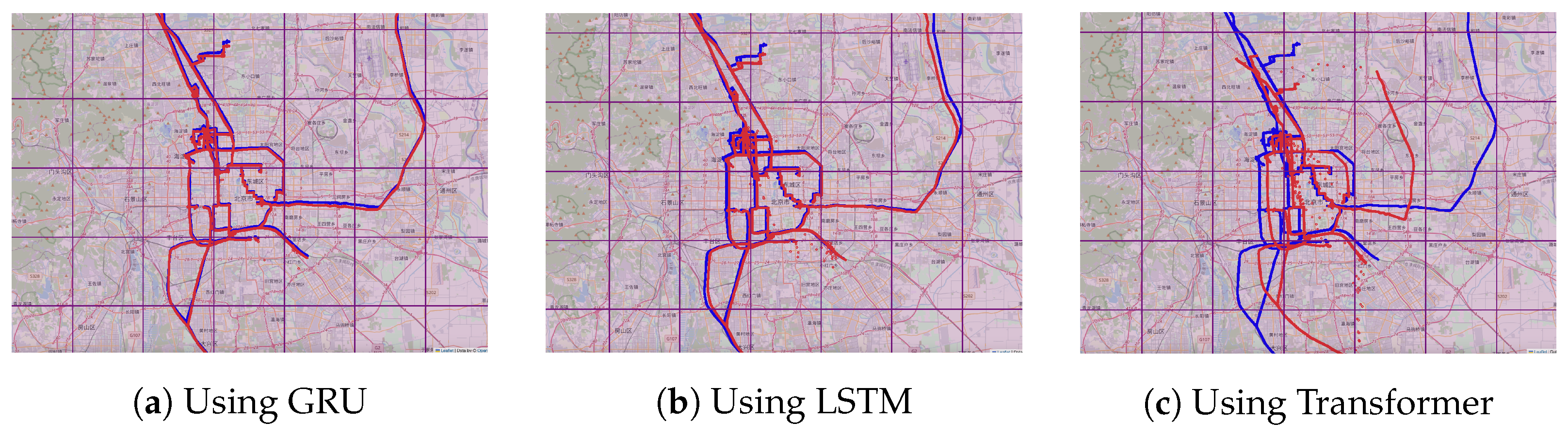
As shown in Figure 11, the LSTM and GRU models outperform in predicting the trajectory compared to the actual trajectory of a randomly selected volunteer from the Geolife dataset. The performance of the three mobility models is evaluated by using the four performance metrics discussed in Section 5.3. As shown in

Table 2. Comparison of the accuracy of the models.

Model	Mean	Std. Deviation	95% Confidence Interval
LSTM	0.9179	0.1018	[0.8949, 0.9375]
GRU	0.9234	0.1078	[0.8977, 0.9449]
Transformer	0.8151	0.1737	[0.7879, 0.8416]

, the mean accuracy in predicting the future region of all the volunteers by the GRU-based mobility model is 0.9234, which is higher than the accuracy of prediction achieved by the LSTM and Tranformer-based mobility models. Similarly, as shown in

Table 3. Comparison of the RMSE of the models.

Model	Mean	Std. Deviation	95% Confidence Interval
LSTM	0.0063	0.0067	[0.0047, 0.0081]
GRU	0.0053	0.0053	[0.0043, 0.0065]
Transformer	0.0135	0.0102	[0.0107, 0.0162]

and

Table 4. Comparison of the geodesic distance (in miles) of the models.

Model	Mean	Std. Deviation	95% Confidence Interval
LSTM	0.5298	0.55213	[0.3992, 0.6819]
GRU	0.4448	0.44495	[0.3609, 0.5437]
Transformer	1.1440	0.8467	[0.9025, 1.3732]

, the GRU-based model outperforms the LSTM and Transformer in both mean RMSE and mean geodesic distance (in miles).

A possible reason why LSTM and GRU outperformed the Transformer model for this task is that, while they excel at capturing long-range dependencies, they struggle with sequences that have strong local temporal dependencies, as seen in sequential time-stamped location behavior data. It is to be noted that the monitoring task is a real-time control task. A possible explanation for why LSTM and GRU outperformed the Transformer in this task relates to the characteristics of the dataset and the structural properties of the models. The coverage zone prediction problem is largely dominated by short-term temporal transitions, where the next location is strongly influenced by recent movement history. Recurrent models such as GRU and LSTM process data sequentially and maintain a continuously updated hidden state, which naturally emphasizes recent observations and temporal continuity. This makes them well-suited for modeling local sequential patterns in mobility data. In addition, the relatively limited size of the dataset favors models with fewer parameters, as they are less prone to overfitting and can generalize more effectively under constrained data conditions. While Transformers are powerful for modeling long-range dependencies and benefit from parallelized training, their higher capacity may not provide additional advantages in this specific real-time spectrum monitoring scenario. Consequently, recurrent models outperform the Transformer under the experimental conditions considered.

Finally, as shown in

Table 5. Comparison of the execution time (in seconds) of the models.

Model	Mean	Std. Deviation	95% Confidence Interval
LSTM	311.521	448.359	[220.0406, 404.1181]
GRU	299.428	411.566	[211.3795, 390.4299]
Transformer	320.636	453.153	[223.1013, 394.0880]

, the GRU-based model takes an average of $299.428$ s to train and test on the location trace of each user, compared to LSTM, which takes an average of $311.521$ s, and the Transformer, which takes an average of $320.636$ s. This is expected as GRUs train faster due to their simpler architecture. Therefore, based on these performance metrics, a GRU-based mobility model is preferable to use compared to the LSTM and Transformer models. However, it is necessary to determine if the difference in performance between the three models is statistically significant.

As shown in

Table 6. Paired t-test results of LSTM versus Transformer.

Accuracy		RMSE		Geodesic Distance		Execution Time
t	p-Value	t	p-Value	t	p-Value	t	p-Value
6.443	$\mathbf{2}.\mathbf{84}\times {\mathbf{10}}^{-\mathbf{9}}$	−8.88	$\mathbf{1}.\mathbf{05}\times {\mathbf{10}}^{-\mathbf{14}}$	−9.0	$\mathbf{5}.\mathbf{39}\times {\mathbf{10}}^{-\mathbf{15}}$	−0.705	0.482

and

Table 7. Paired t-test results of GRU versus Transformer.

Accuracy		RMSE		Geodesic Distance		Execution Time
t	p-Value	t	p-Value	t	p-Value	t	p-Value
8.078	$\mathbf{7}.\mathbf{26}\times {\mathbf{10}}^{-\mathbf{13}}$	−10.2	$\mathbf{8}.\mathbf{69}\times {\mathbf{10}}^{-\mathbf{18}}$	−10.523	$\mathbf{1}.\mathbf{52}\times {\mathbf{10}}^{-\mathbf{18}}$	−1.594	0.114

, the p-values of mean accuracy, RMSE, and geodesic distance are lesser than the significance value of 0.05. This implies that there is a significant difference in the performance of the Transformer-based mobility model when compared to LSTM and GRU-based mobility models. Since the mean accuracy is lesser and the RMSE and geodesic distance of the Transformer-based model are higher than that of both LSTM and GRU, it can be concluded that Transformers perform poorly on these three metrics when compared to LSTM and GRU. As shown in

Table 8. Paired t-test results of LSTM versus GRU.

Accuracy		RMSE		Geodesic Distance		Execution Time
t	p-Value	t	p-Value	t	p-Value	t	p-Value
−0.559	0.577	2.953	0.004	3.107	0.002	1.419	0.159

, the p-values of mean accuracy and execution time are both greater than the significance value of 0.05. This implies that the null hypothesis cannot be rejected and thus there is no significant difference in the performance of the LSTM and GRU models in terms of mean accuracy and execution time. However, for mean RMSE and geodesic distance, the p-values are 0.004 and 0.002, respectively, which are both less than the significance value of 0.05. This implies that the performances of GRU and LSTM are significantly different in terms of mean RMSE and geodesic distance. Since the average RMSE and geodesic distance of GRU are less than that of LSTM (as shown in Table 3 and Table 4), it is concluded that the GRU-based model performs significantly better than LSTM in terms of RMSE and geodesic distance. Lower RMSE and geodesic distance indicate a more accurate trajectory prediction of volunteers. For spectrum monitoring, it is more important to predict the future region of a volunteer in low execution time than to predict the exact future trajectory of a volunteer. Therefore, both LSTM and GRU can be interchangeably used to model volunteer mobility for spectrum monitoring.

7. Conclusions

With the exponential increase in the use of wireless services, the demand for an additional spectrum is steadily on the rise. To address the spectrum scarcity problem, there is a need for spectrum sharing. To this end, the FCC proposed Dynamic Spectrum Access (DSA), wherein licensed frequency bands, when idle, are utilized by unlicensed users. As spectrum sharing becomes more intense with more stakeholders, we can expect an increase in the number of potentially enforceable events [5]. Hence, the success of shared-spectrum networks depends on the ability to effectively monitor the spectrum and enforce spectrum access policies. In this work, a crowdsourced approach is applied to effectively monitor the spectrum. This requires the selection of crowdsourced volunteers to ensure effective coverage of all the regions in the entire enforcement area over a period of time. For this purpose, we divide each enforcement region into coverage zones and aim to select volunteers who ensure effective coverage of each zone. In this paper, we focus on (i) defining and developing an approach to assess the capability of a volunteer to cover a zone in a spectrum enforcement region, as well as (ii) applying and analyzing deep learning models for predicting the availability of a volunteer in a given coverage zone. Three deep learning models, LSTM, GRU, and Transformer, are explored, and a simulation-based study using real-world data is performed to assess their performances. The results of the simulation show that LSTM and GRU outperform the Transformer model. Furthermore, the results indicate that the difference between the performance of LSTM and GRU is not statistically significant in terms of volunteer future coverage zone prediction accuracy. The execution time of both models is also comparable. Therefore, either model is suitable for access rights enforcement in shared-spectrum wireless networks.

In the proposed framework, volunteers may register with information that is not genuine. For example, if the location that a volunteer shares is not accurate, then it can hinder the recruitment of qualified volunteers, thereby hampering effective spectrum enforcement. Another example of a lapse in security can occur when a volunteer registers with a fake identity. Information related to the crowdsourced volunteers must be verified to avoid adverse issues arising from security lapses. This is an area that we plan to address in future research. Volunteers who are recruited to monitor the spectrum may collude with the spectrum intruders and utilize the spectrum illegally themselves. Such collaboration can cause additional overheads that hinder the overall detection of spectrum misuse in a geographical region of enforcement. Collusions can additionally be of varying types—volunteer–volunteer collusion, volunteer–intruder collusion, and collusion among multiple volunteers and intruders. This is also an area of research that we haven’t explored yet and plan to address in the future.

References

1. 5 GHz Band Overview—fcc.gov. Available online: https://www.fcc.gov/wireless/bureau-divisions/mobility-division/35-ghz-band/35-ghz-band-overview (accessed on 3 August 2024).
2. Han, H.; Wang, X.; Gu, F.; Li, W.; Cai, Y.; Xu, Y.; Xu, Y. Better late than never: GAN-enhanced dynamic anti-jamming spectrum access with incomplete sensing information. IEEE Wirel. Commun. Lett. 2021, 10, 1800–1804. [Google Scholar]
3. Li, W.; Chen, J.; Liu, X.; Wang, X.; Li, Y.; Liu, D.; Xu, Y. Intelligent dynamic spectrum anti-jamming communications: A deep reinforcement learning perspective. IEEE Wirel. Commun. 2022, 29, 60–67. [Google Scholar] [CrossRef]
4. Weiss, M.B.; Altamimi, M.; McHenry, M. Enforcement and spectrum sharing: A case study of the 1695–1710 mhz band. In Proceedings of the 8th International Conference on Cognitive Radio Oriented Wireless Networks; IEEE: Piscataway, NJ, USA, 2013; pp. 7–12. [Google Scholar]
5. Das, D.; Znati, T.; Weiss, M.B. Efficient Monitoring of Dynamic Spectrum Access for Robust and Reliable Detection of Unauthorized Access. In Proceedings of the MILCOM 2022–2022 IEEE Military Communications Conference (MILCOM); IEEE: Piscataway, NJ, USA, 2022; pp. 729–734. [Google Scholar]
6. Das, D.; Rose, J.S.; Znati, T.; Bustamante, P.; Weiss, M.; Gomez, M.M. Spectrum misuse detection in cooperative wireless networks. In Proceedings of the 2020 IEEE 17th Annual Consumer Communications & Networking Conference (CCNC); IEEE: Piscataway, NJ, USA, 2020; pp. 1–6. [Google Scholar]
7. Das, D.; Znati, T.; Weiss, M.B.; Gomez, M.M.; Bustamante, P.; Rose, J.S. Matchmaking of volunteers and channels for dynamic spectrum access enforcement. In Proceedings of the GLOBECOM 2020–2020 IEEE Global Communications Conference; IEEE: Piscataway, NJ, USA, 2020; pp. 1–6. [Google Scholar]
8. Das, D. A Framework for Intelligent Crowdsourced Enforcement of Access Rights in Shared Spectrum Networks. Doctoral Dissertation, University of Pittsburgh, Pittsburgh, PA, USA, 2024. [Google Scholar]
9. Afuah, A.; Tucci, C.L. Reflections on the 2022 AMR decade award: Crowdsourcing as a solution to distant search. Acad. Manag. Rev. 2023, 48, 597–610. [Google Scholar] [CrossRef]
10. Pohlisch, J. Internal Crowdsourcing at SAP. In Proceedings of the European Conference on Innovation and Entrepreneurship; Academic Conferences International Limited: Reading, UK, 2019; p. 1201-XXIV. [Google Scholar]
11. Pohlisch, J. An introduction to internal crowdsourcing. In Internal Crowdsourcing in Companies; Springer: Cham, Switzerland, 2021; p. 15. [Google Scholar]
12. Xerandy, X.; Ai, F.; Znati, T.; Comfort, L.K.; Ismail, F.A. Device-to-Device Communication: A Scalable, Socially Aware, Land-Based Infrastructure to Support Community Resilience in Disaster Events. In Hazardous Seas: A Sociotechnical Framework for Early Tsunami Detection and Warning; Island Press: Columbia, WA, USA, 2023; p. 91. [Google Scholar]
13. Nelson, T.; Roy, A.; Ferster, C.; Fischer, J.; Brum-Bastos, V.; Laberee, K.; Yu, H.; Winters, M. Generalized model for mapping bicycle ridership with crowdsourced data. Transp. Res. Part C Emerg. Technol. 2021, 125, 102981. [Google Scholar] [CrossRef]
14. Glińska, E.; Kiryluk, H.; Ilczuk, K. Crowdsourcing initiatives in city management: The perspective of Polish local governments. Ekon. ŚRodowisko 2022, 82, 287–311. [Google Scholar]
15. Muller, C.; Chapman, L.; Johnston, S.; Kidd, C.; Illingworth, S.; Foody, G.; Overeem, A.; Leigh, R. Crowdsourcing for climate and atmospheric sciences: Current status and future potential. Int. J. Climatol. 2015, 35, 3185–3203. [Google Scholar]
16. Palacios-Marqués, D.; Gallego-Nicholls, J.F.; Guijarro-García, M. A recipe for success: Crowdsourcing, online social networks, and their impact on organizational performance. Technol. Forecast. Soc. Change 2021, 165, 120566. [Google Scholar] [CrossRef]
17. Jin, X.; Sun, J.; Zhang, R.; Zhang, Y.; Zhang, C. Specguard: Spectrum misuse detection in dynamic spectrum access systems. IEEE Trans. Mob. Comput. 2018, 17, 2925–2938. [Google Scholar] [CrossRef]
18. Li, M.; Yang, D.; Lin, J.; Tang, J. SpecWatch: A framework for adversarial spectrum monitoring with unknown statistics. Comput. Netw. 2018, 143, 176–190. [Google Scholar]
19. Lin, J.; Li, M.; Yang, D.; Xue, G.; Tang, J. Sybil-proof incentive mechanisms for crowdsensing. In Proceedings of the IEEE INFOCOM 2017—IEEE Conference on Computer Communications; IEEE: Piscataway, NJ, USA, 2017; pp. 1–9. [Google Scholar]
20. Chen, Y.; Xiong, Y.; Wang, Q.; Yin, X.; Li, B. Stable matching for spectrum market with guaranteed minimum requirement. In 18th ACM International Symposium on Mobile Ad Hoc Networking and Computing; ACM: New York, NY, USA, 2017; pp. 1–10. [Google Scholar]
21. Mazlan, N.; Syed Ahmad, S.S.; Kamalrudin, M. Volunteer selection based on crowdsourcing approach. J. Ambient. Intell. Humaniz. Comput. 2018, 9, 743–753. [Google Scholar] [CrossRef]
22. Liu, S.; Greenstein, L.J.; Trappe, W.; Chen, Y. Detecting anomalous spectrum usage in dynamic spectrum access networks. Ad Hoc Netw. 2012, 10, 831–844. [Google Scholar]
23. Wang, S.L.; Tsai, T.H.; Chung, W.H. The novel crowdsourcing algorithm for cooperative spectrum sensing. In Proceedings of the 2018 IEEE International Symposium on Dynamic Spectrum Access Networks (DySPAN); IEEE: Piscataway, NJ, USA, 2018; pp. 1–5. [Google Scholar]
24. Mallery, C.; Ganachari, D.; Fern, J.; Smeeding, L.; Robinson, S.; Moon, M.; Lavallee, D.; Siegel, J. Innovative Methods in Stakeholder Engagement: An Environmental Scan; American Institutes for Research: Rockville, MD, USA, 2012. [Google Scholar]
25. Leimeister, J.M.; Huber, M.; Bretschneider, U.; Krcmar, H. Leveraging crowdsourcing: Activation-supporting components for IT-based ideas competition. J. Manag. Inf. Syst. 2009, 26, 197–224. [Google Scholar] [CrossRef]
26. Alexander Hars, S.O. Working for free? Motivations for participating in open-source projects. Int. J. Electron. Commer. 2002, 6, 25–39. [Google Scholar] [CrossRef]
27. Hertel, G.; Niedner, S.; Herrmann, S. Motivation of software developers in Open Source projects: An Internet-based survey of contributors to the Linux kernel. Res. Policy 2003, 32, 1159–1177. [Google Scholar] [CrossRef]
28. Lakhani, K.R.; Wolf, R.G. Why hackers do what they do: Understanding motivation and effort in free/open source software projects. In Perspectives on Free and Open Source Software; MIT Press: Cambridge, MA, USA, 2005. [Google Scholar]
29. Lerner, J.; Tirole, J. Some simple economics of open source. J. Ind. Econ. 2002, 50, 197–234. [Google Scholar] [CrossRef]
30. Rochman, M.I.; Sathya, V.; Nunez, N.; Fernandez, D.; Ghosh, M.; Ibrahim, A.S.; Payne, W. A comparison study of cellular deployments in Chicago and Miami using apps on smartphones. In 15th ACM Workshop on Wireless Network Testbeds, Experimental Evaluation & Characterization; ACM: New York, NY, USA, 2022; pp. 61–68. [Google Scholar]
31. Abdul-Quddoos, T.; Sharmin, T.; Li, X.; Qian, L. Transmitter Identification and Protocol Categorization in Shared Spectrum via Multi-Task RF Classification at the Network Edge. In Proceedings of the 2025 IEEE International Conference on Communications Workshops (ICC Workshops); IEEE: Piscataway, NJ, USA, 2025; pp. 2168–2173. [Google Scholar]
32. Bhatti, F.A.; Khan, M.J.; Selim, A.; Paisana, F. Shared Spectrum Monitoring Using Deep Learning. IEEE Trans. Cogn. Commun. Netw. 2021, 7, 1171–1185. [Google Scholar] [CrossRef]
33. Liu, S.; Wang, Q.; Qin, Z.; Zhang, W.; Wang, J.; Ma, X. IRS Assisted Decentralized Learning for Wideband Spectrum Sensing. In Proceedings of the International Symposium on Intelligent Computing and Networking; Springer: Berlin/Heidelberg, Germany, 2025; pp. 507–523. [Google Scholar]
34. Fernando, X.; Lăzăroiu, G. Spectrum sensing, clustering algorithms, and energy-harvesting technology for cognitive-radio-based internet-of-things networks. Sensors 2023, 23, 7792. [Google Scholar] [CrossRef]
35. Atimati, E.; Nyasulu, T.; Crawford, D.; Stewart, R. Resource Management in Dynamic Shared Spectrum Networks. In Proceedings of the 2025 IEEE International Symposium on Dynamic Spectrum Access Networks (DySPAN); IEEE: Piscataway, NJ, USA, 2025; pp. 13–19. [Google Scholar]
36. Chigaba, A.W.; Nleya, S.M.; Velempini, M.; Dube, S.S. A Multi-Objective Genetic Algorithm–Deep Reinforcement Learning Framework for Spectrum Sharing in 6G Cognitive Radio Networks. Appl. Sci. 2025, 15, 9758. [Google Scholar] [CrossRef]
37. Jia, M.; Zhang, X.; Sun, J.; Gu, X.; Guo, Q. Intelligent Resource Management for Satellite and Terrestrial Spectrum Shared Networking toward B5G. IEEE Wirel. Commun. 2020, 27, 54–61. [Google Scholar] [CrossRef]
38. Shang, B.; Wang, Z.; Li, X.; Yang, C.; Ren, C.; Zhang, H. Spectrum Sharing in Satellite-Terrestrial Integrated Networks: Frameworks, Approaches, and Opportunities. IEEE Netw. 2025; early access. [CrossRef]
39. Testi, E.; Giorgetti, A. Wireless Network Analytics for the New Era of Spectrum Patrolling and Monitoring. IEEE Wirel. Commun. 2024, 31, 230–236. [Google Scholar] [CrossRef]
40. Hao, C.; Wan, X.; Feng, D.; Feng, Z.; Xia, X.G. Satellite-Based Radio Spectrum Monitoring: Architecture, Applications, and Challenges. IEEE Netw. 2021, 35, 20–27. [Google Scholar] [CrossRef]
41. Zheng, S.; Han, T.; Jiang, Y.; Ge, X. Smart Contract-Based Spectrum Sharing Transactions for Multi-Operators Wireless Communication Networks. IEEE Access 2020, 8, 88547–88557. [Google Scholar] [CrossRef]
42. Zhang, H.; Leng, S.; Yin, H.; Yu, S. Intelligent Consensus Enhanced Spectrum Sharing in Heterogeneous Wireless Networks. IEEE Internet Things J. 2024, 11, 30939–30952. [Google Scholar] [CrossRef]
43. Camelo, M.; Mennes, R.; Shahid, A.; Struye, J.; Donato, C.; Jabandzic, I.; Giannoulis, S.; Mahfoudhi, F.; Maddala, P.; Seskar, I.; et al. An AI-Based Incumbent Protection System for Collaborative Intelligent Radio Networks. IEEE Wirel. Commun. 2020, 27, 16–23. [Google Scholar] [CrossRef]
44. Zhang, Y.; Hu, G.; Cai, Y. Proactive spectrum monitoring for suspicious wireless powered communications in dynamic spectrum sharing networks. China Commun. 2021, 18, 119–138. [Google Scholar] [CrossRef]
45. Janu, D.; Singh, K.; Kumar, S. Machine learning for cooperative spectrum sensing and sharing: A survey. Trans. Emerg. Telecommun. Technol. 2022, 33, e4352. [Google Scholar] [CrossRef]
46. Ahmad, W.S.H.M.W.; Radzi, N.A.M.; Samidi, F.S.; Ismail, A.; Abdullah, F.; Jamaludin, M.Z.; Zakaria, M.N. 5G Technology: Towards Dynamic Spectrum Sharing Using Cognitive Radio Networks. IEEE Access 2020, 8, 14460–14488. [Google Scholar] [CrossRef]
47. Malakar, G. Cognitive Radio Networking: An Intelligent Approach to Spectrum Utilization. Int. J. Future Mob. Wirel. Netw. 2025, 3, 44470. [Google Scholar] [CrossRef]
48. Song, H.; Bai, J.; Yi, Y.; Wu, J.; Liu, L. Artificial Intelligence Enabled Internet of Things: Network Architecture and Spectrum Access. IEEE Comput. Intell. Mag. 2020, 15, 44–51. [Google Scholar] [CrossRef]
49. Sankhe, K.; Belgiovine, M.; Zhou, F.; Angioloni, L.; Restuccia, F.; D’Oro, S.; Melodia, T.; Ioannidis, S.; Chowdhury, K. No radio left behind: Radio fingerprinting through deep learning of physical-layer hardware impairments. IEEE Trans. Cogn. Commun. Netw. 2019, 6, 165–178. [Google Scholar] [CrossRef]
50. Verma, G.; Yu, P.; Sadler, B.M. Physical layer authentication via fingerprint embedding using software-defined radios. IEEE Access 2015, 3, 81–88. [Google Scholar] [CrossRef]
51. Reus-Muns, G.; Upadhyaya, P.S.; Demir, U.; Stephenson, N.; Soltani, N.; Shah, V.K.; Chowdhury, K.R. Senseoran: O-ran-based radar detection in the cbrs band. IEEE J. Sel. Areas Commun. 2023, 42, 326–338. [Google Scholar] [CrossRef]
52. Anderson, A.; Wang, X.; Baker, K.R.; Grunwald, D. Systems for spectrum forensics. In 2nd International Workshop on Hot Topics in Wireless; ACM: New York, NY, USA, 2015; pp. 26–30. [Google Scholar]
53. Park, J.M.; Reed, J.H.; Beex, A.; Clancy, T.C.; Kumar, V.; Bahrak, B. Security and enforcement in spectrum sharing. Proc. IEEE 2014, 102, 270–281. [Google Scholar] [CrossRef]
54. Barbeau, M.; Hall, J.; Kranakis, E. Detection of rogue devices in bluetooth networks using radio frequency fingerprinting. In 3rd IASTED International Conference on Communications and Computer Networks; ACTA Press: Calgary, AB, Cananda, 2006; pp. 4–6. [Google Scholar]
55. Kim, K.; Spooner, C.M.; Akbar, I.; Reed, J.H. Specific emitter identification for cognitive radio with application to IEEE 802.11. In Proceedings of the IEEE GLOBECOM 2008–2008 IEEE Global Telecommunications Conference; IEEE: Piscataway, NJ, USA, 2008; pp. 1–5. [Google Scholar]
56. Remley, K.; Grosvenor, C.A.; Johnk, R.T.; Novotny, D.R.; Hale, P.D.; McKinley, M.; Karygiannis, A.; Antonakakis, E. Electromagnetic signatures of WLAN cards and network security. In Fifth IEEE International Symposium on Signal Processing and Information Technology, 2005; IEEE: Piscataway, NJ, USA, 2005; pp. 484–488. [Google Scholar]
57. Danev, B.; Luecken, H.; Capkun, S.; El Defrawy, K. Attacks on physical-layer identification. In Third ACM Conference on Wireless Network Security; ACM: New York, NY, USA, 2010; pp. 89–98. [Google Scholar]
58. Goergen, N.; Clancy, T.C.; Newman, T.R. Physical layer authentication watermarks through synthetic channel emulation. In Proceedings of the 2010 IEEE Symposium on New Frontiers in Dynamic Spectrum (DySPAN); IEEE: Piscataway, NJ, USA, 2010; pp. 1–7. [Google Scholar]
59. Wang, X.; Wu, Y.; Caron, B. Transmitter identification using embedded pseudo random sequences. IEEE Trans. Broadcast. 2004, 50, 244–252. [Google Scholar] [CrossRef]
60. Tan, X.; Borle, K.; Du, W.; Chen, B. Cryptographic link signatures for spectrum usage authentication in cognitive radio. In Proceedings of the Fourth ACM Conference on Wireless Network Security; ACM: New York, NY, USA, 2011; pp. 79–90. [Google Scholar]
61. Kumar, V.; Li, H.; Park, J.M.J.; Bian, K. Crowd-sourced authentication for enforcement in dynamic spectrum sharing. IEEE Trans. Cogn. Commun. Netw. 2019, 5, 625–636. [Google Scholar] [CrossRef]
62. Muldoon, C.; O’Grady, M.J.; O’Hare, G.M. A survey of incentive engineering for crowdsourcing. Knowl. Eng. Rev. 2018, 33, e2. [Google Scholar] [CrossRef]
63. Zhao, Y.; Zhu, Q. Evaluation on crowdsourcing research: Current status and future direction. Inf. Syst. Front. 2014, 16, 417–434. [Google Scholar] [CrossRef]
64. Mao, A.; Kamar, E.; Chen, Y.; Horvitz, E.; Schwamb, M.; Lintott, C.; Smith, A. Volunteering versus work for pay: Incentives and tradeoffs in crowdsourcing. Aaai Conf. Hum. Comput. Crowdsourcing 2013, 1, 94–102. [Google Scholar] [CrossRef]
65. Bénabou, R.; Tirole, J. Incentives and prosocial behavior. Am. Econ. Rev. 2006, 96, 1652–1678. [Google Scholar] [CrossRef]
66. McIntosh, D.; Al-Nuaimy, W.; Ataby, A.A.; Sandall, I.; Selis, V.; Allen, S. Gamification approaches for improving engagement and learning in small and large engineering classes. Int. J. Inf. Educ. Technol. 2023, 13, 1328–1337. [Google Scholar] [CrossRef]
67. Morschheuser, B.; Hamari, J.; Maedche, A. Cooperation or competition–When do people contribute more? A field experiment on gamification of crowdsourcing. Int. J. Hum.-Comput. Stud. 2019, 127, 7–24. [Google Scholar] [CrossRef]
68. Ortiz-Rojas, M.; Chiluiza, K.; Valcke, M.; Bolanos-Mendoza, C. How gamification boosts learning in STEM higher education: A mixed methods study. Int. J. Stem Educ. 2025, 12, 1. [Google Scholar] [CrossRef]
69. Azizan, A.; Aris, H. A Hybrid Crowdsourcing Incentive Mechanism Based on Users’Preference. In 6th International Conference on Computing and Informatics; IEEE: Piscataway, NJ, USA, 2017; pp. 363–368. [Google Scholar]
70. Zheng, Y.; Zhang, L.; Xie, X.; Ma, W.Y. Mining interesting locations and travel sequences from GPS trajectories. In 8th International Conference on WORLD Wide Web; ACM: New York, NY, USA, 2009; pp. 791–800. [Google Scholar]
71. Zheng, Y.; Li, Q.; Chen, Y.; Xie, X.; Ma, W.Y. Understanding mobility based on GPS data. In 10th International Conference on Ubiquitous Computing; ACM: New York, NY, USA, 2008; pp. 312–321. [Google Scholar]
72. Zheng, Y.; Xie, X.; Ma, W.Y. GeoLife: A collaborative social networking service among user, location and trajectory. IEEE Data Eng. Bull. 2010, 33, 32–39. [Google Scholar]
73. Rumelhart, D.E.; Hinton, G.E.; Williams, R.J. Learning representations by back-propagating errors. Nature 1986, 323, 533–536. [Google Scholar] [CrossRef]
74. Cho, K.; Van Merriënboer, B.; Gulcehre, C.; Bahdanau, D.; Bougares, F.; Schwenk, H.; Bengio, Y. Learning phrase representations using RNN encoder-decoder for statistical machine translation. arXiv 2014, arXiv:1406.1078. [Google Scholar] [CrossRef]
75. Hochreiter, S.; Schmidhuber, J. Long short-term memory. Neural Comput. 1997, 9, 1735–1780. [Google Scholar] [CrossRef]
76. Vaswani, A.; Shazeer, N.; Parmar, N.; Uszkoreit, J.; Jones, L.; Gomez, A.N.; Kaiser, Ł.; Polosukhin, I. Attention is all you need. In Proceedings of the 31st Conference on Neural Information Processing Systems (NeurIPS 2017), Long Beach, CA, USA, 4–9 December 2017; pp. 6000–6010. [Google Scholar]
77. Robusto, C.C. The cosine-haversine formula. Am. Math. Mon. 1957, 64, 38–40. [Google Scholar] [CrossRef]
78. Dauni, P.; Firdaus, M.; Asfariani, R.; Saputra, M.; Hidayat, A.; Zulfikar, W. Implementation of Haversine formula for school location tracking. J. Phys. Conf. Ser. 2019, 1402, 077028. [Google Scholar] [CrossRef]
Figure 1. Spectrum Enforcement Framework Architecture and Components.
Network 06 00019 g001
Figure 2. Components of the Access Enforcement Computational Infrastructure.
Network 06 00019 g002
Figure 3. Volunteer registration methodology.
Network 06 00019 g003
Figure 4. Classification of volunteer attributes.
Network 06 00019 g004
Figure 5. Interaction between a volunteer and different components of the Access Enforcement Computational Infrastructure for updating the dynamic and behavioral attributes of the volunteer.
Network 06 00019 g005
Figure 6. Functionality of the Adjudication Component in the Access Enforcement Computational Infrastructure.
Network 06 00019 g006
Figure 7. Sample of the volunteer selection strategy for the initial two Monitoring Intervals, M I 0 and M I 1 .
Network 06 00019 g007
Figure 8. Coverage zones in enforcement region, r.
Network 06 00019 g008
Figure 9. Volunteer zone prediction for selection in a Monitoring Interval.
Network 06 00019 g009
Figure 10. Sliding windows for training and testing LSTM and GRU models.
Network 06 00019 g010
Figure 11. Comparison of the predicted trajectories (in red) versus actual trajectories (in blue) of a volunteer using different deep learning models. We observe that the RNN-based models in (a,b) exhibit better performance in trajectory prediction compared to transformers (as shown in (c)).
Network 06 00019 g011