Design and Analysis of an Effective Architecture for Machine Learning Based Intrusion Detection Systems

Abstract

The increase in new cyber threats is the result of the rapid growth of using the Internet, thus raising questions about the effectiveness of traditional Intrusion Detection Systems (IDSs). Machine learning (ML) technology is used to enhance cybersecurity in general and especially for reactive approaches, such as traditional IDSs. In several instances, it is seen that a single assailant may direct their efforts towards different servers belonging to an organization. This behavior is often perceived by IDSs as infrequent attacks, thus diminishing the effectiveness of detection. In this context, this paper aims to create a machine learning-based IDS model able to detect malicious traffic received by different organizational network interfaces. A centralized proxy server is designed to receive all the incoming traffic at the organization’s servers, scan the traffic by using the proposed IDS, and then redirect the traffic to the requested server. The proposed IDS was evaluated by using three datasets: CIC-MalMem-2022, CIC-IDS-2018, and CIC-IDS-2017. The XGBoost model showed exceptional performance in rapid detection, achieving 99.96%, 99.73%, and 99.84% accuracy rates within short time intervals. The Stacking model achieved the highest level of accuracy among the evaluated models. The developed IDS demonstrated superior accuracy and detection time outcomes compared with previous research in the field.

1. Introduction

In the realm of online security, the predominant concern is in the occurrence of security breaches, which mostly stem from the act of intrusion. In the event of a single error or unauthorized access, it is possible for an individual to swiftly gain control over or erase data pertaining to the computer and system architecture [1]. In addition, a centralized network design may exhibit increased susceptibility to several forms of security breaches, including unauthorized access, data breaches, and distributed denial-of-service (DDoS) assaults. Furthermore, the occurrence of an intrusion may lead to substantial financial ramifications and compromised computer transactions, ultimately leading to a dearth of data in the context of a cyber digital conflict. The system may be negatively impacted by security failures [2,3]. According to [4], the implementation of IDSs is crucial to mitigating failures. In a broad sense, an IDS is designed to identify and respond to network assaults by actively monitoring the software and hardware configurations of a given network [5]. By doing so, it plays a crucial role in safeguarding against cyber threats [6]. There exist many challenges linked with IDSs, including the incapability to identify novel assaults, a very low rate of accurate detection, and the need to mitigate false alarm occurrences. Furthermore, it is worth noting that anomalous intrusion detection approaches are still facing ongoing challenges in terms of achieving consistent performance improvements [7]. The use of ML and deep learning methodologies is often seen in the context of augmenting the efficiency of IDSs [7] as advanced technological systems with the ability to access and retrieve relevant data. Due to their ability to extract important information from vast datasets in an automated manner, ML models have garnered significant attention in academic circles. This is mostly due to their effectiveness as a tool for knowledge retrieval. By using a large number of training data, IDSs may attain high levels of perceptiveness, while ML models demonstrate satisfactory generalization capabilities in the realm of attack detection. One further benefit of ML technology is its ease of design and development, as highlighted by [8]. Ensuring network security for an organization is especially important given the widespread use of the Internet for inter-organizational and inter-company communication, which amplifies the potential for the dissemination of attacks and threats among these entities. Conventional IDSs may be inadequate in detecting novel infiltration attempts. Moreover, the network intrusion detection system (NIDS) receives different traffic since every IDS is installed in other sub-networks of the organization. In many cases, the same attacker may target multiple organization servers seen by each IDS as seldom attacks, decreasing the detection rate. Therefore, this situation poses challenges in accurately discerning genuine dangers and promptly implementing appropriate measures. Organizations have to use more advanced solutions, such as IDSs based on ML, in order to enhance their security stance. The idea is to create an ML-based IDS model to detect malicious traffic received by different organization network interfaces. A centralized proxy server is created to receive all the traffic from the organization’s servers, scan the traffic by using the proposed IDS, and then redirect the traffic to the requested server. The key features of our contributions are as follows:

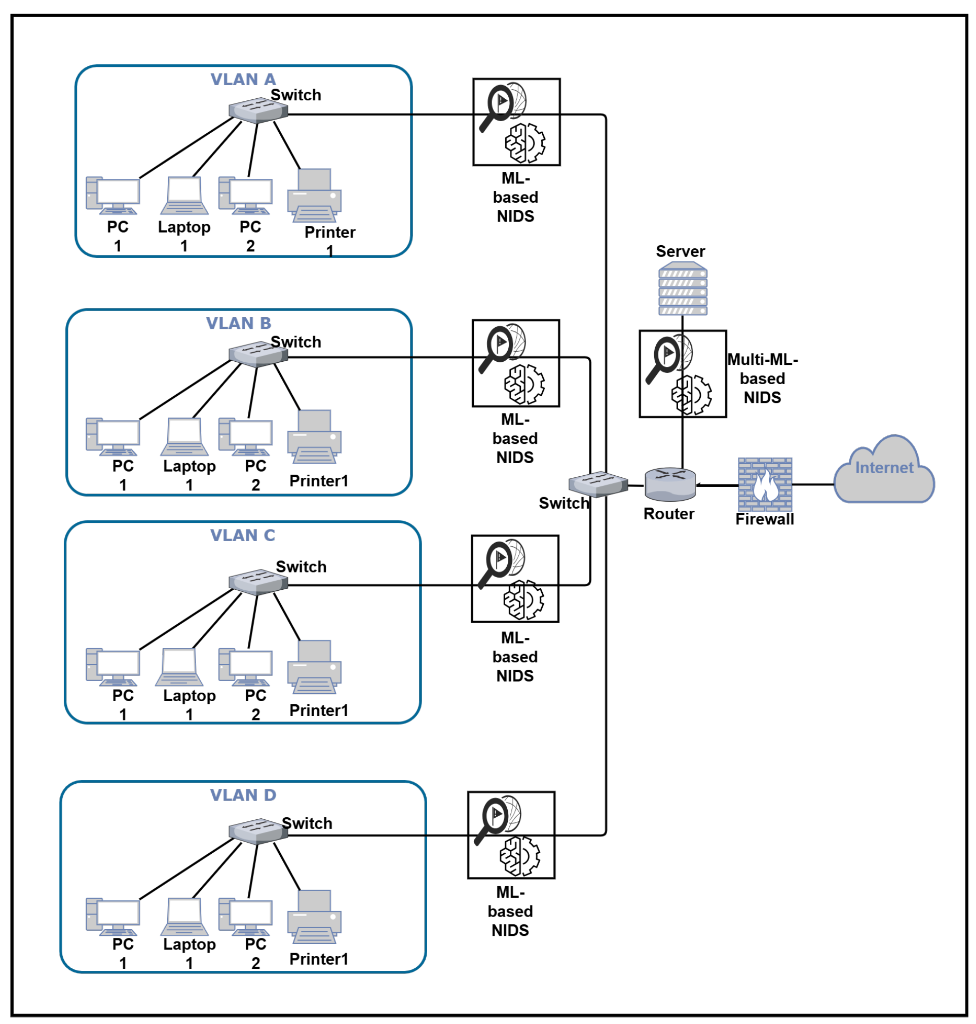
• A novel centralized network architecture based on a multi-model IDS based on traffic load. The model is more realistic since organizations have prime time or specific events.
• In the proposed model, global traffic inspection occurs before traffic is sent to the central server and other sub-networks of the organization.
• We analyze the results of the AdaBoost, Voting, Stacking, Support Vector Machine, Random Forest, and XGBoost 3.0.0 models on the datasets CIC-MalMem-2022, CIC-IDS-2018, and CIC-IDS- 2017.
• We compare the best models with existing IDSs.

The following is the description of the remaining structure of this research paper: Section 2 discusses previous works on IDSs and ML techniques. Section 3 describes the novel centralized network architecture and introduces the used datasets and ML models. An analysis of the experimental results is presented in Section 4, which also compares them with the findings of previous studies. Finally, Section 5 concludes the paper with recommendations for further research.

2. Literature Review

In cybersecurity, detection accuracy is the primary challenge for ML-based IDSs. This literature review aims to lay the foundation for the development of an innovative architecture for ML-based IDSs.

2.1. Intrusion Detection Systems

IDSs are used to monitor network traffic behavior or analyze data generated by a host in order to detect and identify any unauthorized entry attempts that compromise security. These technologies serve as the primary means of protection for the industry against possible cybersecurity attacks. Upon the discovery of an assault, an alarm is promptly sent. The core principles of IDSs are centered on the actions of monitoring, detecting, and responding to any instances of unauthorized activity. An intrusion refers to the unauthorized use, exploitation, and manipulation of computer systems by individuals, both external and internal, in a manner that is not sanctioned. To safeguard a computer system or computer network, it is essential for an IDS to first detect and recognize malicious assaults targeting host devices or network systems [9].

There are two categorization approaches that may be used for IDSs, which are distinguished depending on the data source and detection [10]. Each approach has distinct characteristics. There are two distinct groups of data source-based methods: host-based IDSs (HIDSs) and network-based IDSs (NIDSs). In addition, it is worth noting that there are two distinct categories of detection-based approaches, namely, anomaly-based and signature-based detection [11]. IDSs pose four notable challenges [12], which are low detection rate, false alarm rate, response time, and unbalanced dataset. In order to overcome these challenges [13], ML, data mining [14], and statistical methods are widely used with IDSs.

2.2. Machine Learning

The significance of integrating ML into the field of cybersecurity has escalated due to its ability to rapidly assess and detect various forms of threats from a vast number of events [15]. Moreover, ML is a methodology used to automate the procedure of constructing analytical models by using data, whereby the models acquire the ability to make judgments via learning [16]. There are two primary categories of ML algorithms, with the first category consisting of shallow models. The second approach under consideration is deep learning, as mentioned by [17]. According to [18], the categorization of learning algorithms is based on the manner in which data are used, resulting in four distinct types: unsupervised, semi-supervised, supervised, and reinforcement learning. In contrast, there exist four distinct categories of ML that possess independent learning characteristics. These categories include information-based learning techniques, similarity-based learning techniques, probability-based learning techniques, and error-based learning techniques. Collectively, these categories are commonly referred to as the ML family [19,20].

Table 1. Overview of ML families and algorithms.

ML Family	Description	Algorithms
Information-based learning	Building models based on information theory concepts.	Random Tree, Random Forest, J48, HoeffdingTree, REPTree, and Decision Stump
Similarity-based learning	Comparing known and unknown things or measuring the degree of similarity between past and future events.	k-NN and k-means (Simple k-means, Canopy, and Hierarchical)
Probability-based learning	Developing a model based on measuring the probability of an event occurring.	Naïve Bayes
Error-based learning	Building a model that minimizes the total error by using a set of training instances.	SVM, Logistic Regression, Perceptron, Winnow, and deep learning

presents a comprehensive overview of the ML family and its corresponding algorithms.

Table 2. Advantages and disadvantages of ML families.

ML Family	Advantages	Disadvantages
Information-based learning	Interpretable and straightforward. Captures interaction between descriptive and defining features.	Prone to overfitting. Not suitable for concepts that change over time (requires retraining).
Similarity-Based learning	Easy to interpret. Handles a wide range of descriptive features.	Slow prediction speed, especially with large datasets. Lower accuracy compared with other approaches.
Probability-based learning	Fast and efficient. Suitable for categorical input variables.	Assumes feature independence (often unrealistic). Requires significant data and careful development based on assumptions.
Error-based learning	Can model complex relationships between variables. Panel data can provide more variability and less collinearity.	Finding optimal weights requires searching a large space. Panel data models have limitations like heterogeneity correlation.

presents the advantages and disadvantages of ML.

ML has made restorative diagnosis, cancer detection, computer vision, social media marketing, smart transportation, and gaming possible [21]. ML techniques are preferred over traditional rules-based learning algorithms for human intervention in various industries. As a result, ML has a significant role in cybersecurity [21]. In addition to identifying malicious activities and vulnerabilities in real time, it also enhances the overall security posture of the system [21].

2.3. Related Work

This section discusses several recent research papers that investigate ML-based IDSs and deep learning-based IDSs.

2.3.1. Information-Based Learning Techniques

Attou et al. [22] enhanced IDSs by using ML algorithms to monitor resources, services, and networks, detecting cloud attacks based on monitoring data. The model accuracy rate achieved 99.99 % on the BoT-IoT dataset, which includes RF algorithms for intrusion prediction and graphic visualization. However, the study has limitations, as it only uses the Bot-IoT and NSL-KDD datasets for evaluation and does not examine various cloud computing deployment models or compare different ML algorithms on system performance. Saheed et al. [23] developed an IoT IDS to detect abnormal behavior in an IoT network using ML methods and feature dimensional reduction. They applied preprocessing steps using min–max to normalize the data and then applied PCA to select the most relevant features from the 49 attributes on the UNSWNB15 dataset. After trimming the dataset, XGBoost was trained on it. The study did not evaluate other IoT network typologies. Seth et al. [24] presented a hybrid feature selection approach designed to decrease the complexity of the model, prediction latency, and attack prediction performance without adversely affecting the model. They used LightGBM, a lightweight gradient-boosting framework, on the CIC-IDS 2018 dataset. With the proposed feature selection, prediction latency was reduced by 45.52 % to 2.25 %, and construction time was reduced by 52.68 % to 17.94 %. With LightGBM, the model achieved 97.73 % accuracy, 99.3 % sensitivity, 99.3 % precision, and a short prediction delay. According to the proposed model, accuracy and precision were improved by 1.5 % and 3 %, respectively, over the existing model.

2.3.2. Similarity-Based Learning Techniques

Ding et al. [25] proposed a solution to sparse data by using a DAN method to extract features from data. They created data of minority classes within overlapped regions by using TACGAN, which uses information loss to align minority class data with the original data. The data filtering module removes noise after the model is completed. The accuracy results for KDDCUP99, UNSW-NB15, and CICIDS2017 were 93.53%, 92.39%, and 95.86%, respectively. Another study by Dini and Saponara [26] developed an application using K-nearest neighbors and artificial neural networks (ANNs) to analyze local area network traffic flow. They used a US Air Force-emulated LAN to obtain authenticated TCP/IP dump data. This technique performed better than PCA by selecting the cosine of similarity to compare observations in the training set using a feature reduction approach based on multidimensional scaling. The datasets examined accurately represented LAN traffic in military applications, with the ANN’s accuracy of 99.23 % and the KNN’s accuracy of 99.57 %. However, current IDSs face issues such as false positives, low detection rates, and inability to detect newly launched attacks or unbalanced datasets. The study examined only a limited number of ML techniques, and a comparison with other techniques would be interesting.

2.3.3. Probability-Based Learning Techniques

Hnamte et al. [27] proposed using the Dice similarity coefficient to select features for intrusion detection in IoT networks. They categorized transactions as positive or negative, aiming to select optimal features to prevent intrusion. The model improves classification performance by indicating if network infrastructure transactions can be accessed. IoT-Sentinel evaluates the model output, while a Naïve Bayes classifier scales it. However, the study has limitations in evaluating scalability, robustness, and overhead and assumes independent and equally distributed training data, which is unrealistic in IoT networks with dynamic sources. Also, Onah et al. [28] proposed GANBADM for security research in fog computing environments. The model uses Genetic Algorithm Wrapper and Naïve Bayes classifiers for feature selection. The results may not apply to other datasets, as the model was constructed on the NSL-KDD dataset, achieving 99.73% accuracy.

2.3.4. Error-Based Learning Techniques

Baniasadi et al. [29] developed a method using Deep Convolutional Neural Networks (DCNNs) to detect IoT device attacks. They also developed a neighborhood search-based particle swarm optimization algorithm (NSBPSO) for enhanced exploration and exploitation capabilities. The model was trained by using the NSBPSO-DCNN algorithm, achieving a 99.41% performance on the test dataset and 98.86% on the training dataset. However, due to computational costs, this study may not be feasible for real-time intrusion detection due to IoT systems’ lack of data. Naveed et al. [30] proposed a new method for detecting IDSs due to low detection rates. The two-stage implementation process involves selecting features like chi-squared, ANOVA, and PCA. A Deep Neural Network model was developed on the NSL-KDD dataset for classifying traffic into normal and abnormal modes. However, the framework could have performed better on other datasets. A data imbalance can lead to incorrect classification of attack data, as average data are outnumbered by attack data, causing a difficult challenge. Moreover, Ponmalar and Dhanakoti [31] proposed an IDS that tackles the complexities of big data, security data, and big data environments. The system identified nine new assault types in the UNSW-NB15 dataset with 96.29% accuracy, enhancing classification accuracy. Network traffic is analyzed by using SVM, and features are selected by using CGO. However, the study has limitations, such as the need for a large number of labeled data, which are costly and difficult to obtain. Additionally, Ullah and Mahmoud [32] developed a new IDS model by combining the RFE feature selection approach and CNN algorithms. As part of the assessment of the accuracy of the model, the MQTT-IoT-IDS2020 dataset, which comprises three layers of CNNs and multiclass classifications, was used. A CNN was the only deep learning model considered in this study, although other models, including RNNs, LSTM, and GRUs, may be more suitable for IoT networks.

2.3.5. Hybrid Models

Hnamte and Hussain [33] has developed a new IDS model using RFE feature selection and CNN algorithms. The model uses three layers of CNNs and multiclass classification, with accuracy determined on the MQTT-IoT-IDS2020 dataset. They used only CNNs in their research study. The model was trained on the CICIDS2018 and Edge IIoT datasets, with 100% accuracy rates with and without GPUs. In Edge IIoT datasets with a GPU, the accuracy rates was 99.46%, and without a GPU, it was 99.62%. However, the model requires considerable training time and has limitations due to the costs associated with computationally expensive training data, as well as the quality of the data used in training. With the increasing sophistication and number of attacks, anomaly-based NIDSs may become more difficult to use when handling a large number of data, making them an alternative for IoT networks. Talukder et al.’s [34] research work aimed to integrate deep learning and ML to improve detection rates while maintaining reliability. They tested various algorithms, including KNN, RF, DT, CNN, ANN, MLP, and deep learning. According to the SMOT algorithm’s balance of data and XGBoost, the RF model was the most accurate. They used two datasets to evaluate their model: KDDCUP’99 and CIC-MalMem-2022. It is recommended that the proposed model consider environmental factors such as network traffic and bandwidth. Also, Balyan et al. [35] developed a hybrid NIDS model that uses improved Random Forest techniques (IRF), genetic algorithms, and particle swarm optimization (EGA-PSO) techniques. By using a multi-objective function, the model reduces dimensions, identifies key features, enhances the GA, selects the best feature, and improves fitness results. Iterative training removes less critical features, incorporates decision trees, and monitors classification accuracy to avoid overfitting. The HNIDS approach achieves 98.97% accuracy in BCC and 88.14% accuracy in MCC, outperforming SVM, RF, LR, NB, and LDA on the NSL-KDD datasets. The study measured four parameters, accuracy, TPR, precision, and FPR, without considering CPU utilization and time. Akshay Kumaar et al. [36] used deep learning techniques in ImmuneNet to recognize attacks. The framework achieved high performance and accuracy through the use of multiple feature engineering processes, oversampling methods, and hyperparameter optimization. Data from CIC IDS 2017, CIC IDS 2018, and CIC Bell DNS 2021 were compared by using XGB, Random Forest, Decision Trees, and Logistic Regression. On the CIC Bell DNS 2021 dataset, ImmuneNet achieved an accuracy rate of 99.19%. However, the model cannot learn independently, requiring significant time and effort. The study by Patil et al. [37] used RF, SVM, DT, and an ensemble Voting classifier to create an IDS with 96.25% accuracy on the CICIDS-2017 dataset. It highlighted the importance of trust in human–machine interaction success. The Learnable Machine Interface made predictions easily understood, facilitating model selection, trust assessment, and the improvement of models. However, the study used a single dataset, which may not reflect real-world scenarios or data distributions, and did not address privacy, accountability, or trust issues in intrusion detection. Also, Rincy N. and Gupta [38] explored ML techniques for analyzing assaults. They proposed CAPPER, which uses high-accuracy algorithms with low false positive rates to select the best feature subsets for hybrid NID-Shield NIDSs. The algorithm uses CFS and Wrappers to select feature subsets, ensuring a free-from-duplicate set. Filtering and wrapping approaches are combined to produce accurate and high-quality feature sets. The hybrid CAPPER algorithm achieved a performance accuracy of 99.89% on the UNSW NB15 and NSL-KDD20% datasets. However, the model was not evaluated against a recent dataset to determine if it reflects the latest attack trends. A hybrid anomaly detection approach based on Naïve Bayes, Random Forest, and J48 (C4.5) using Deep Neural Networks and Classical Autoencoders is presented in the study by Dutta et al. [39]. The model has an accuracy rate of 91.29%, significantly higher than previous methods. However, the study is based on a single dataset, which should be more recent. The rapid growth of IoT environments and increasing threats necessitate the assistance of existing ML algorithms to identify new attacks, as existing algorithms need to adapt to the growing threat landscape. In Liu et al. [40], a hybrid anomaly detection system incorporating Deep Neural Networks and Classical Autoencoders was proposed. Based on the UNSW-NB15 benchmark dataset, the model was found to be significantly more accurate than previous models, with an accuracy rate of 91.29%. A single dataset was used in the study, which should have been of a more recent date. Since IoT environments are rapidly growing, existing machine learning algorithms are insufficient for detecting new threats, making the proposed model more appropriate for research in the future. Aldallal and Alisa [41] suggested using hybrid IDS techniques in a cloud environment along with GAs and SVM. The hybrid IDS method categorizes network data into normal and abnormal behavior by using a GA. Based on the KDD CUP 99 dataset, the proposed model achieved a 99.3% accuracy level. However, other datasets or recent attacks may affect the accuracy of the proposed model.

2.3.6. SDN Models

Recently, Software-Defined Networking (SDN) has gained popularity as a way to overcome traditional system limitations by controlling the network through one sophisticated piece of software. The SDN system will simplify network management and improve programmability by separating control and data planes. Furthermore, the recommended strategy would provide SDN protection that is more precise, efficient, and scalable than current techniques, thereby overcoming the limitations of current techniques. Many businesses use network detection algorithms to identify and organize harmful traffic. However, it is difficult to identify these algorithms in unbalanced datasets [42]. Chaganti et al. [43] developed a method for detecting network threats in an SDN-Internet of Things environment by using an IDS model-based LSTM algorithm. The algorithm employs T-SNE-based learning, which is derived from DL models over hidden layers. Based on the SDN-IoT dataset, LSTM models achieved an accuracy rate of 97.1%. However, real-time attack detection requires a large number of labeled data. Alzahrani and Alenazi [44] proposed methods for detecting and identifying SDN attacks as part of the attack detection and identification techniques. The following ML models were employed to detect attacks: DT, RF, and XGBoost. An accuracy rate of 95% was achieved on the NSL-KD dataset. Only one dataset was used, which may need to be updated to include current attacks. Javeed et al. [45] demonstrated that deep learning-enabled, SDN-enabled approaches can enhance the effectiveness, scaling, and cost-effectiveness of threat detection within IoT environments. The hybrid model was trained and tested by using the Cu-BLSTM and Cu-DNNGRU classifiers, which achieved 99.87% accuracy. Even though the proposed model was tested on a limited dataset, it has not yet been tested on datasets with different characteristics. For the detection and mitigation of MR-DDoS attacks in an SDN environment, six ML algorithms were employed: RT, REP Tree, SVM, J48, and MLP. As outlined by Perez-Diaz et al. [46], their method utilizes a modular architecture that is very flexible. MLP has an accuracy rate of 95%. Tests and evaluations were conducted on (CIC) DoS datasets.

2.4. Summary

This study identifies four challenges associated with IDSs: low detection rates, false alarm rates, response times, and unbalanced datasets. Several limitations exist both in data source methods and in detection methods. These challenges can be addressed by three detection techniques: ML, data mining, and statistical techniques. In this study, ML will serve as a detection technique. According to advantages and disadvantages, a hybrid model achieves the highest accuracy result, as demonstrated in [33,34], as an outcome of related work, where 100% accuracy was achieved. However, when probability-based learning is used, the accuracy result is lower, as shown in in [27]; the proposed model’s accuracy was 89.7%. The accuracy of information-based learning and error-based learning is always over 98%. Additionally, feature selection will significantly impact the accuracy result, as demonstrated by the research study in [28], where the accuracy result of the proposed model is 99.73%. Furthermore, the feature selection method can have a significant effect on the accuracy of the ML model, as shown in the following related papers: [33,34,35,36,37,38,39]; the method in each falls under the hybrid model approaches, but they differ in accuracy. Both feature selection and parameter selection can significantly impact the model’s accuracy. In all cases, SDNs show an accuracy of 95% or greater. The literature review considers no specific network architecture for applying ML-based IDSs. However, this study considers the network architecture the principal component for applying ML-based IDSs. Also, the related works provided one-layer security and did not consider the organizations’ requirements if they were under prime time or special event conditions. Most related studies test one ML model on multiple datasets or one dataset trained with multiple models, so there needs to be more explicit information about whether the results are accurate. Moreover, most of the mentioned related works are unrelated to specific domains, such as cloud computing or the Internet of Things, so this field has been left as N/A.

Table 3. Summary of LR.

Ref.	Year	Domain	Method	Algorithms	Dataset	Feat. Sel.	Acc.	Limitations
Attou et al. [22]	2023	CC	Information	RF	BoT-IoT	Graphic Vis.	99.99%	Only Bot-IoT/NSL-KDD datasets. No cloud model examination. No ML algorithm comparison
Hnamte and Hussain [33]	2023	N/A	Hybrid	CNN, BiLSTM, and DNN	CICIDS2018	CNN	100%	Substantial training time required. High computational costs. Increased attack complexity.
Chaganti et al. [43]	2023	SDN-IoT	SDN	LSTM	SDN-IoT	t-SNE	97.1%	Needs large number of labeled data for real-time attack detection.
Talukder et al. [34]	2023	N/A	Hybrid	RF	CIC-MalMem-2022	XGBoost	100%	Does not consider environmental factors like network traffic.
Saheed et al. [23]	2022	IoT	Information	XGBoost	UNSW-NB15	PCA	99.99%	Uses only one dataset.
Baniasadi et al. [29]	2022	IoT	Error	DCNN	BoT-IoT	NSBPSO	98.86%	High computational costs. IoT systems lack data.
Balyan et al. [35]	2022	N/A	Hybrid	IRF	NSL-KDD	EGA-PSO	99.97%	Uses only one dataset.
Naveed et al. [30]	2022	Network Traffic	Error	DNN	NSL-KDD	Chi-squared, ANOVA, and PCA	99.73%	Data imbalance may cause incorrect classification.
Ding et al. [25]	2022	N/A	Similarity	KNN	CIC-IDS-2017	N/A	95.86%	High computational impact on efficiency and scalability.
Hnamte et al. [27]	2022	IoT	Probability	Naïve Bayes	IoT Sentinel	DSC	89.7%	Scalability, robustness, and overhead concerns. Needs large number of labeled data.
Ponmalar and Dhanakoti [31]	2022	Big Data	Error	SVM	UNSW-NB15	CGO	96.29%	Requires costly labeled data acquisition.
Akshay Kumaar et al. [36]	2022	N/A	Hybrid	ImmuneNet	CIC Bell DNS 2021	All Features	99.19%	Model requires significant time for learning.
Patil et al. [37]	2022	N/A	Hybrid	Voting	CIC-IDS-2017	Correlation Heatmap	96.25%	Single-dataset limitations.
Dini and Saponara [26]	2021	LAN	Similarity	KNN	LAN traffic (USAF)	MDS	99.57%	Limited ML model comparison.
Rincy N and Gupta [38]	2021	Network	Hybrid	NB, RF, J48, and CFS	NSL-KDD20%	CAPPER	99.90%	Untested on recent attack datasets.
Dutta et al. [39]	2021	N/A	Hybrid	DNN	UNSW-NB15	CAE	99.979%	Single dataset. High computational cost.
Ullah and Mahmoud [32]	2021	IoT	Error	CNN	MQTT-IoT-IDS2020	RFE	99.99%	Latency/processing power challenges.
Alzahrani and Alenazi [44]	2021	SDN	SDN	XGBoost	NSL-KDD	N/A	95.95%	Single dataset used.
Javeed et al. [45]	2021	SDN-IoT	SDN	Cu-BLSTM and Cu-DNNGRU	CIC-IDS-2018	N/A	99.87%	Single-dataset limitation.
Liu et al. [40]	2021	N/A	Hybrid	K-means, RF, LSTM, and CNN	CIC-IDS-2017	N/A	99.91%	Lacks recent attack data.
Aldallal and Alisa [41]	2021	CC	Hybrid	SVM	KDD CUP 99	GA	99.3%	Outdated dataset used.
Onah et al. [28]	2021	Fog	Probability	Naïve Bayes	NSL-KDD	GA Wrapper	99.73%	Dataset recency issues.
Seth et al. [24]	2021	IoT	Information	LightGBM	CIC-IDS-2018	RF and PCA	97.73%	Single-dataset limitation.
Perez-Diaz et al. [46]	2020	SDN	SDN	MLP	CIC DoS	N/A	95%	Dataset recency issues.

shows the summary of related work. Consequently, a novel centralized network architecture based on a multi-model IDS is proposed, called multi-model IDS based on traffic load. Further, the following datasets will be used in this study: CIC-MalMem-2022, a recent dataset; the CIC-IDS-2018 and CIC-IDS-2017 datasets, the most commonly used in related studies. In addition to this, the CIC-MalMem-2022, CIC-IDS-2018, and CIC-IDS-2017 datasets serve as valuable resources for researchers involved in intrusion detection and malware analysis. As a result of their real-world representation, diversity of attack types, labeled data, public accessibility, and status as benchmarking standards, they are widely used to develop and evaluate new security solutions. Finally, several learning approaches will be used for this experiment, including hybrid models, information-based learning techniques, and error-based learning techniques. as they achieve high levels of accuracy. The following are the learning approaches and algorithms that will be used in the experiments:

• Hybrid models: The Stacking classifier and the Voting classifier enable different estimators to predict the result.
• Information-based learning techniques: AdaBoost is a powerful and versatile meta-algorithm particularly useful for cybersecurity applications as it can handle imbalanced and noisy datasets [47]. Random Forest is the most used in related studies, and XGBoost is one of the most powerful gradient-boosting algorithms available [48]. Generally, tree-based algorithms such as RF, AdaBoost, and XGbbost have demonstrated high efficiency and effectiveness in handling binary and categorical data and identifying complex feature relationships. Various ML applications use these algorithms, such as classification, regression, and anomaly detection.
• Error-based learning techniques: Support Vector Machine: Researchers commonly use SVM algorithms because of their versatility, robustness, and capability to handle complex data. They are particularly good at handling classification problems but can also be used for regression and anomaly detection.

This study aims to address the limitations presented in Table 3 by examining three datasets that contain the most recent attacks to ensure the effectiveness of the model and using those datasets with different ML models. The study provides two-layer security to ensure privacy and security.

3. Proposed Architecture: Multi-Model IDS Based on Traffic Load

A new centralized network architecture that utilizes a multi-model IDS based on traffic load has been proposed to ensure security and privacy, as shown in Figure 1. The proposed architecture provides two-layer security. The first layer contains two ML-based IDS models and is activated according to the amount of incoming network traffic. The first model takes less time, so it is faster but less accurate than the second model. The second model has a single model and is more accurate than the first but is less speedy and takes more time. The proposed architecture allows organizations to monitor incoming traffic and encrypt sensitive data while restricting access to authorized users only. The IDS models used in this study incorporate both signature-based detection and behavior-based detection, which reduces the false alarm rate and increases accuracy. First, signature-based detection is applied to the traffic; if no signatures are found, behavior-based detection is applied. By combining signature detection and behavior detection, both sensitivity and specificity can be maintained for network traffic. Signature detection enhances specificity, thereby reducing false alarm rates, and behavior detection enhances sensitivity, increasing accuracy.

3.1. Proposed Architecture Components

According to Figure 1, the proposed architecture consists of different components:

• Firewalls: Firewalls can be configured to block traffic from malicious IP addresses by manually adding these addresses to the firewalls’ blocklist; this can be accomplished by configuring the firewalls to block traffic from malicious IP addresses via an IPS (intrusion prevention system).
• Routers and switches: Configured to collect and report statistics on network traffic. Identifying the amount and type of traffic passing through these devices may help determine the volume and type of traffic on the network. In addition, the routers are configured with a threshold value for network traffic.
• Multi-model ML-based NIDS (first layer): This ensures a centralized global view and inspection of the incoming traffic at the different organization servers and contains two types of ML-based IDSs: the first model focuses on the fast inspection of traffic, and the second model focuses on high accuracy.
• ML-based NIDS (second layer): This model is highly accurate. It inspects all traffic before it is distributed to the server that requests it.

3.2. Proposed Architecture Data Flow

An organization’s incoming network traffic from the WAN will first be inspected by the firewalls, which can block the IPs that contain malicious traffic; this can be accomplished by configuring the IPS to block traffic from malicious IP addresses by adding these addresses manually to the IPS’s blocklist. An IPS is a comprehensive security solution that not only detects but also actively prevents various forms of cyber threats by combining the functionality of both IDSs and firewalls.

Before network traffic is distributed to the sub-networks of the organization, global inspection will first be performed through a multi-model IDS, so there are two models for ML-based IDSs. Each IDS model will work according to the traffic entering the network. To calculate traffic on the network, routers and switches are configured to collect and report network traffic statistics. The amount and type of traffic passing through these devices may help determine the volume and type of traffic on the network. The amount of traffic serves as the threshold for choosing the best model; the network administrator assigns the threshold value. As long as traffic remains higher than the threshold value, the fastest model will be active; for example, network traffic is higher than the threshold value during prime time or on specific occasions within the organization. If network traffic falls below the threshold value, the model with the highest accuracy will be active. After choosing the best model to inspect and detect the traffic, the traffic will then be distributed to the sub-networks of the organization. The IDS placed in these sub-networks of the organization is based on a model with high accuracy in detecting malicious activity. Algorithm 1 and Algorithm 2 describe how the proposed architecture works. A multi-model IDS based on traffic load can also be applied to SDNs, although suitability will depend on several factors, including network complexity, hardware requirements, and application requirements [49].

Algorithm 1 Assess network traffic.

1: import psutil   2: function get_network_traffic   3:     interfaces ← psutil.net_io_counters(pernic=True)   4:     network_traffic ← 0   5:     for all interface ∈ interfaces do   6:         network_traffic ← network_traffic + interfaces[interface].bytes_recv + interfaces[interface].bytes_sent   7:     end for   8:     return network_traffic   9: end function 10: network_traffic ← get_network_traffic() 11: print “The current network traffic is” network_traffic “bytes”.

Algorithm 2 Select the best model.

1: import pandas as pd   2: import pickle   3: Load model1 into the variable model1   4: Load model2 into the variable model2   5: function select_model([)data, threshold]   6:     traffic ← get_network_traffic()   7:     if traffic > threshold then   8:         prediction ← model1.predict(data)   9:     else 10:         prediction ← model2.predict(data) 11:     end if 12:     return prediction 13: end function 14: sample ← pd.read_csv(‘testFeatures.csv’) 15: prediction ← select_model(sample, 1,000,000) 16: print “The prediction is” prediction

The steps of Algorithm 1 are as follows: First, the psutil module is imported, providing an interface to the operating system’s processes and information. The next function, get_network_traffic(), returns the current network traffic. As the first step, it performs the psutil.net_io_counters(pernic=True) method, which returns a dictionary of network interfaces that indicate how many bytes were received and sent on each interface. After iterating over the dictionary of interfaces, the function adds the bytes_recv and bytes_sent attributes for each interface to the network_traffic variable. Finally, the function returns the network_traffic variable. The final line of code calls the function get_network_traffic(), which prints the current network traffic to the console.

According to Algorithm 2, the first line imports the pickle module, which is used for serializing and deserializing Python 3.10.0 objects. Following these lines, model1, which is the fastest at detecting malicious traffic, and model2, which has the highest accuracy, are loaded from .pkl files created by training the models on datasets containing features and labels. The data and the threshold are the two arguments in the select_model() function. Pandas DataFrames contain the features of the new data point for which a prediction is needed. The threshold is the amount of network traffic used to determine which model to use. The threshold value is controlled by the network admin.

To determine the current network traffic, the function first uses the get_network_traffic() function, as described in Algorithm 1. When the network traffic exceeds the threshold, the function uses model1. Alternatively, the function makes a prediction by using model2. The function then returns the result.

In the final two lines of code, the test data are read from a CSV file, and the select_model() function is called to make the prediction. The prediction is then printed to the console.

3.3. Motivation Behind Using Centralized Network Architecture Approach

Network architectures with a centralized architecture can significantly impact the performance of IDSs that utilize ML algorithms. By implementing a centralized architecture, security threats can be detected more accurately due to improved visibility and control. As a result of the centralized control plane, IDSs based on ML can collect and analyze network data from a wide range of devices to detect anomalous behavior and potential threats [50]. In addition, centralized architectures allow for the uniform enforcement of security policies across the network, reducing the risk of misconfigurations or inconsistencies that may result in false positive alerts from the IDS. By defining and distributing security policies across all network devices, the central controller ensures consistent protection against cyber threats [51]. Moreover, security incidents or breaches can be responded to more rapidly if the network is centralized. By isolating compromised devices, implementing remediation measures, and identifying the affected network areas, the central controller can quickly respond to the affected network areas. By implementing centralized control, security incidents can be responded to more efficiently and effectively, minimizing their impact [51]. In contrast to decentralized network architectures, multiple controllers can present additional challenges in managing and coordinating. Keeping ML-based IDS performing efficiently and effectively can be challenging when it comes to ensuring consistent policy enforcement and efficient communication between controllers and network devices [52]. Furthermore, decentralized architectures may result in additional overhead associated with communication and coordination between controllers, potentially impeding the performance of ML-based IDSs [53]. Decentralized and centralized network architectures are distinct approaches to managing computer systems, networks, and data storage. In centralized network architectures, these networks have the following key differences: a hierarchical structure, which is controlled and managed by a central authority; a single point of failure, which can lead to data breaches, data outages, and censorship; data stored in a central location, resulting in vulnerabilities and privacy concerns; and limited scalability and performance, as the central authority struggles to manage the growing number of data and users [54]. With a decentralized network architecture, a flat structure, where no single entity controls the entire network, increases security and privacy, since data are stored in multiple nodes, increasing its resilience to attacks and censorship and improving its scalability and performance, as it can adapt to an increased number of users and data storage, as well as reducing reliance on a central authority, which can improve the network’s overall resilience [54]. Therefore, centralized and decentralized network architectures can benefit from ML-based IDSs, but the choice will depend on the network’s specific requirements and constraints. While decentralized architectures provide better privacy and resilience, centralized architectures may provide enhanced security and control [54,55]. A summary of the advantages and disadvantages of centralized and decentralized network architectures can be found in

Table 4. Advantages and disadvantages of centralized and decentralized network architectures.

Network Type	Advantages	Disadvantages
Centralized	Easy to manage Efficient resource allocation Strong security	Single point of failure Reduced resilience Reduced user autonomy
Decentralized	Adaptability to failure Reduced censorship Enhanced user autonomy	Increased complexity Difficult consensus mechanisms Limited scalability

. Related works also support the use of centralized network architectures, as shown in the SDN Models subsection of Related Work, where accuracy is consistently greater than 95% in all mentioned studies. SDNs represent an evolving version of the centralized network architecture principle.

3.4. Benchmark Dataset

This section provides an overview of the datasets used in this study. It is recommended that researchers utilize the CIC-MalMem-2022, CIC-IDS-2018, and CIC-IDS-2017 datasets for intrusion detection and malware analysis purposes. The fact that they are based on real-world attacks, are labeled, and are publicly accessible has made them popular tools for developing and evaluating new security solutions. Additionally, there are U2R attacks, such as SQL injections and buffer overflows, and 2L attacks, such as remote login attacks and Trojan horse attacks [56,57,58]. The datasets used in this study contain various types of threats. CIC-MalMem-2022 contains several types of attacks, including U2R attacks, R2L attacks, probe attacks, malware attacks, and botnet attacks [56], while the CIC-IDS-2018 dataset contains probe attacks, such as port scanning, ping sweeps, and network scans. It also contains U2R attacks, such as buffer overflows and SQL injection attacks. Additionally, it contains 2L attacks, such as remote login attacks and Trojan horse attacks [57]. Also, the CIC-IDS-2017 dataset consists of probe attacks, such as port scanning, ping sweeps, and network scans. Additionally, the dataset consists of U2R attacks, such as buffer overflows and SQL injection attacks, and 2L attacks, such as remote login attacks and Trojan horse attacks [58]. In

Table 5. Dataset comparison.

Dataset	Number of Samples	Classes
CIC-MalMem-2022	58,596	Benign, Trojan horse, Ransomware, and Spyware
CIC-IDS-2018	16,232,943	Benign, botnet, DDoS, brute force, DoS, Infiltration, Web Attack, brute force SSH, and Heartbleed
CIC-IDS-2017	2,830,743	Benign, Infiltration, port scanning, DoS, Web Attack, brute force, and bots

, the datasets and attack classes are described in detail. A diagram of the model’s architecture is shown in Figure 2. The process begins with selecting a dataset, followed by data preparation and feature selection based on the dataset. After the data have been split into training and test sets, 80% of them are used for training and 20% for testing. Finally, the ML model is fitted to the training set and then to the test set in order to determine whether the data are benign or malicious.

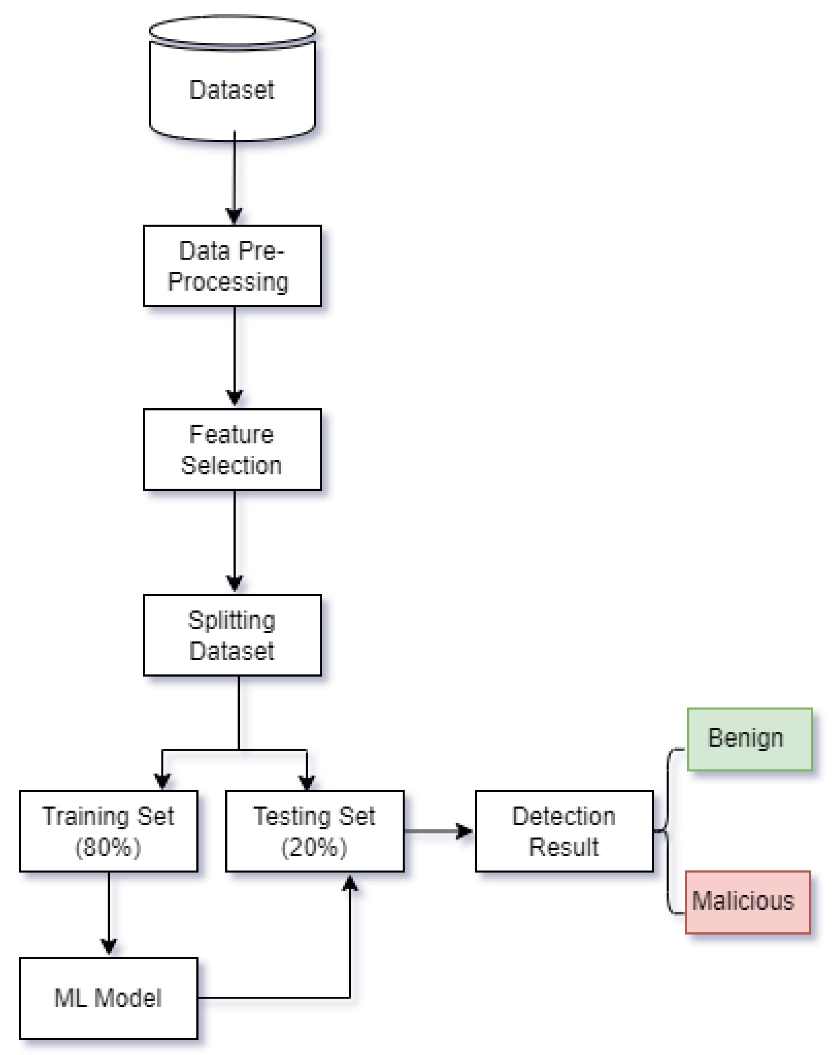
3.5. Data Preprocessing

This research paper uses a subset of the CIC-IDS-2018 and CIC-IDS-2017 datasets for several reasons. First, manageability: smaller datasets are more manageable, especially when computational resources are limited. Secondly, by concentrating on specific aspects of the data relevant to their study, a subset allows researchers to reduce irrelevant information by focusing on relevant data. The use of subsets is helpful for the preliminary testing of hypotheses and algorithms, ensuring more controlled and manageable experiments. Data quality is also enhanced when a smaller subset is cleaned and preprocessed to ensure high data accuracy. Additionally, subsets can assist in maintaining privacy and adhering to legal restrictions, especially if sensitive information is involved. Finally, resource efficiency: analyzing a smaller dataset can save time and resources in terms of computational power and labor [59].

3.5.1. Data Cleaning

For the CIC-MalMem-2022 dataset, firstly, the category column was removed from the dataset since it contains the same data as the class column. The data in both columns consist of benign and malware data. Also, we removed 534 duplicate rows from the dataset. The dataset is divided into two categories, namely, target and features. The target contains the class column, and features contain the rest of the dataset columns.

The CIC-IDS-2018 dataset contains ten separate CSV files. Nine are for malicious data, and the tenth is for benign data. By using the concatenation function, the ten CSV files became one. In addition, only 5000 records were selected from each CSV file because it is a very large dataset. Afterward, the label column was converted into a category that indicates malicious or benign behavior. In the next step, we removed columns dst_ip, src_port, src_ip, and flow_id since they contain 45,000 records with NaN values.

The CIC-IDS-2017 dataset contains eight separate CSV files, each containing benign and malicious records. The eight CSV files were concatenated into one by using the concatenation function. Moreover, only 50,000 records were selected from each CSV file because it is a huge dataset. After this step, the _label column was converted into a category, malicious or benign. We converted the data types of features to float, because some features are numeric, but the data type is object. We set the values of the features to 0 if the value was infinite. Also, we replaced the NaN values with zero.

Table 6. Columns removed from the CIC-IDS-2017 dataset.

Index	Feature Name	Reason
1	_bwd_psh_flags	Contains constant values
2	_bwd_urg_flags	Contains constant values
3	fwd_avg_bytes_bulk	Contains constant values
4	_fwd_avg_packets_bulk	Contains constant values
5	_fwd_avg_bulk_rate	Contains constant values
6	_bwd_avg_bytes_bulk	Contains constant values
7	_bwd_avg_packets_bulk	Contains constant values
8	_bwd_avg_bulk_rate	Contains constant values
9	_fwd_urg_flags	Contains constant values
10	_cwe_flag_count	Contains constant values
11	_rst_flag_count	Contains constant values
12	_ece_flag_count	Contains constant values

shows the columns removed from the dataset because they contain constant values; thus, a total of 13,835 duplicate records were dropped.

3.5.2. Feature Engineering

The following feature engineering techniques were applied to the CIC-IDS-2018 dataset:

• The data type for the timestamp column was converted into the DateTime type, and three new columns, namely, day, month, and year, were added to the dataset. In these three new columns, the value from the timestamp column was taken, and then the timestamp column was dropped.
• The dataset was split into features and the target, and the data types of all feature columns that are objects were converted to numeric. The values of the features were set to 0 if the value was infinite to improve code execution speed without affecting accuracy.

3.5.3. Random Undersampling or Oversampling

The CIC-MalMem-2022 and the CIC-IDS-2017 datasets do not require oversampling or undersampling, in contrast to the CIC-IDS-2018 dataset, in which the malicious class is greater than the benign class, so the RandomUnderSampler was used. The RandomUnderSampler provides a fast, easy method for balancing the data by randomly selecting subsets of data from the targeted categories.

3.5.4. LabelEencoder for Target

We used the LabelEncoder function to encode the categorical data. The value of the class column in the CIC-MalMem-2022 dataset and the values in the label column in the CIC-IDS-2018 and CIC-IDS-2017 datasets were converted into 0 for benign and 1 for malware.

3.5.5. Data Normalization

We used the StandardScaler function to scale the dataset’s features. To standardize the features, the mean should be removed, and the variance should be scaled to one. Also, it provides a simple yet effective way to standardize feature values. We used function transformers to handle the missing data for the Categorical and DateTime features.

3.6. Feature Selection

To conduct ML experiments, it is necessary to evaluate the suitability of various feature selection techniques for different datasets within the field. In ML, feature selection is crucial to identifying the most relevant and informative features in the dataset. Selecting a subset of relevant features in the dataset allows us to improve ML models’ performance, computational complexity, and interpretability [60]. The dataset’s characteristics and specific ML task being performed are affected by which feature selection method will be applied in the dataset. The type of data, whether the data contain noise or irrelevant information, and the features’ distribution all affect feature selection effectiveness [60].

There are two types of feature selection in this study, i.e., SelectKBest and VarianceThreshold:

• Univariate feature selection: SelectKBest uses a statistical test to determine the top-K features. Many types of statistical tests are available, including chi-squared, F-tests, mutual information tests, and others. By selecting the first K features with the highest scores from the input dataset, SelectKBest retains them [61]. SelectKbest uses a univariate feature selection method to determine the strength of the relationship between a response variable and a feature. This method offers a greater understanding of data because of its simplicity and ease of use (though it could be optimized for better generalization because of the simplicity and ease of use of these methods). SelectKBest simplifies the modeling process when working with many features by identifying the most essential features needed to make accurate predictions [61].
• Removing features with low variance: In the VarianceThreshold algorithm, features with variances that do not meet a certain threshold are removed from the analysis. By default, all zero-variance features, which have the same value across all samples, are removed. Variance is typically calculated as the squared distance from the mean divided by the average squared value [62]. The variance of binary data (values of 0 and 1) can be calculated by using the following formula:

  $$Var\left[X\right]=p(1-p)$$

  (1)

  where p indicates the proportion of 1s in the dataset.

The feature selection for the CIC-MalMem-2022 dataset and the CIC-IDS-2017 dataset was conducted by using SelectKBest, where K is 25 in the CIC-MalMem-2022 dataset and K is 30 in the CIC-IDS-2017 dataset. Assigning the value of K is determined by trying different values of K and then evaluating the model’s performance. According to VarianceThreshold, the default value of 0 is recommended. This is because it is necessary to remove features with zero variance, and the CIC-IDS-2018 dataset contains a substantial number of features with zero variance.

There are several benefits to using SelectKBest to select features for intrusion detection tasks. It is a simple, efficient, and effective technique that can enhance the performance of ML algorithms. Since the CIC-IDS-2018 dataset is complex, using VarianceThreshold to select features is preferable. It is an excellent choice for complex datasets because it is simple and efficient and can quickly identify high-variance subsets of features. All features with low variance are excluded from the CIC-IDS-2018 dataset. The threshold value for this experiment is 0. The dataset (features and target) was split into training data with a value of 80% and test data with a value of 20%. The datasets were significantly reduced in size from their original dimensions due to the application of data preprocessing and feature selection methods. Consequently, most of the CIC-MalMem-2022 data lacked relevance, redundancy, and accuracy. Thus, the CIC-MalMem-2022 dataset was reduced to 25, indicating that the remaining features were the most important for predictive modeling.

Despite reducing the new samples to 32,713, a significant portion of the CIC-IDS-2018 dataset lacked variety, relevance, and accuracy. As a result, the number of features was reduced to 72, which indicates that the remaining features are the most key to predictive modeling. Despite the decrease in the number of new samples to 66,757, a significant portion of the CIC-IDS-2017 dataset lacked variety, relevance, and accuracy. Thus, the number of features was reduced to 30, which indicates that the remaining features are the most pertinent to the predictive modeling process.

As a result of this reduction in data size and feature count, several benefits can be obtained, including the following:

• Improved prediction accuracy: As a result of focusing on the most relevant and reliable data, ML algorithms can identify patterns and relationships within the data more accurately, resulting in more accurate predictions [20].
• Minimized computational complexity: Smaller datasets require fewer computational resources, making training and executing ML models more efficient [63].
• Enhanced interpretability: The interpretation of the results is enhanced when fewer features are used, since fewer features make it easier to identify the underlying factors that influence the study’s results [64].
• Reduced overfitting: By reducing the dimensionality of a model, overfitting can be mitigated by eliminating features that do not contribute significantly to predictive power. By reducing the number of features that contribute little to prediction, dimensionality reduction techniques can assist in mitigating overfitting [20].

3.7. Machine Learning Models

This experiment used different learning approaches to train and test the datasets, including hybrid models (Voting and Stacking) because they enable different estimators to predict the result; information-based models (AdaBoost 1.2, Random Forest 1.2, and XGBoost 3.0.0), such as tree-based algorithms have demonstrated excellent efficiency and effectiveness in analyzing binary and categorical data and identifying complex feature relationships. In addition to classification, regression, and anomaly detection, these algorithms are used for various ML applications and error-based learning techniques (SVM) because of their versatility, robustness, and capability to handle complex data. Researchers often use SVM algorithms in classification, regression, and anomaly detection problems.

Classification is a type of learning that uses supervised processes to categorize observations into two or more categories [65]. In contrast to regression, where the target is always a continuous number, categorical regression’s target is always a categorical number [65,66]. Classification requires class labels to be balanced so that all classes are equally important [65]. The purpose of anomaly detection is to distinguish between “normal” and “anomalous” observations [67]. An abnormal observation is typically a rare observation that does not follow the expected pattern of other observations. In addition, this implies that there is likely an imbalance in the dataset [67].

The mentioned models were trained and tested separately on the following datasets: CIC-MalMem-2022, CIC-IDS-2018, and CIC-IDS-2017.

3.8. Performance Evaluation

This section discusses three different approaches to evaluating ML models.

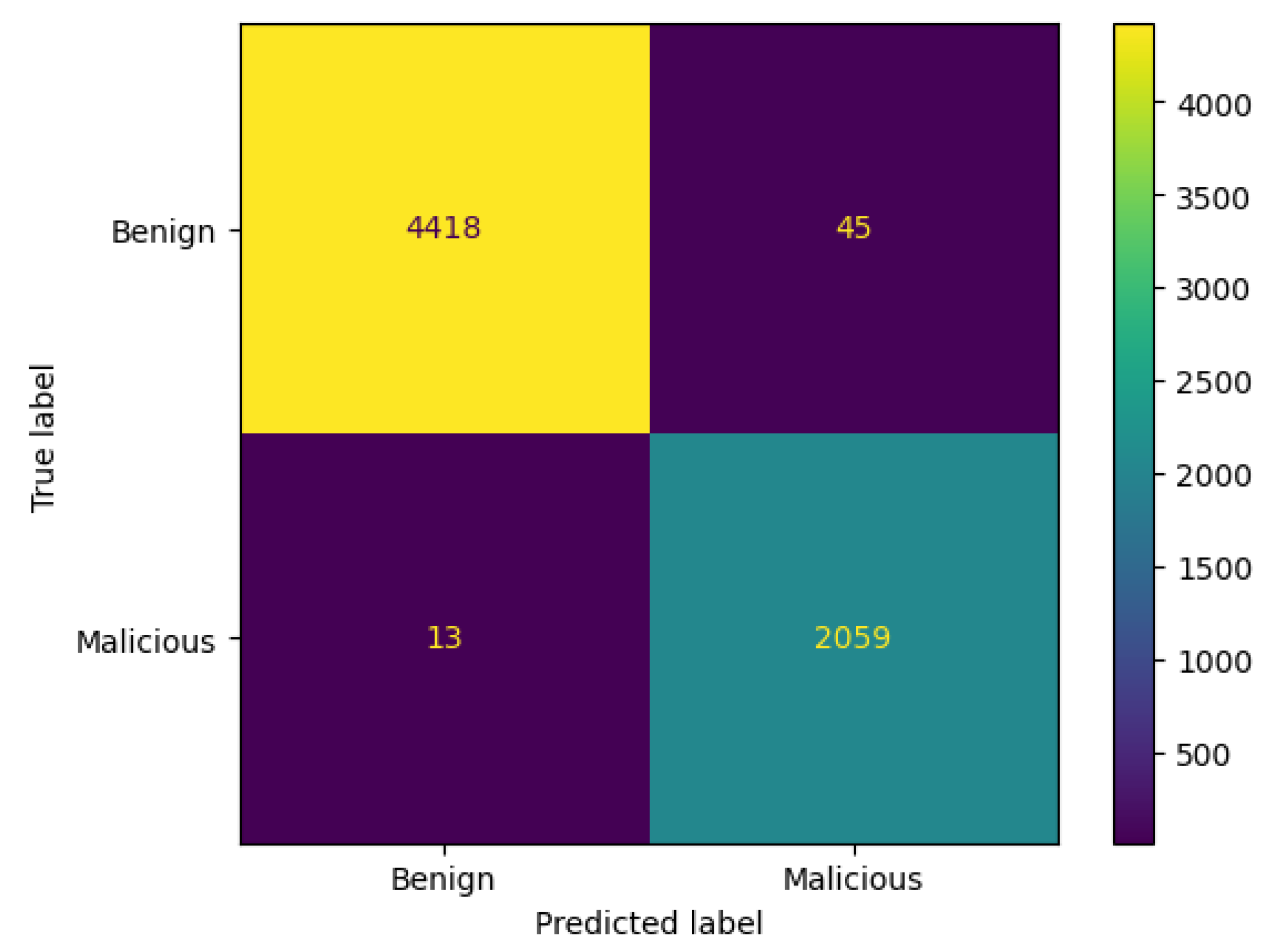
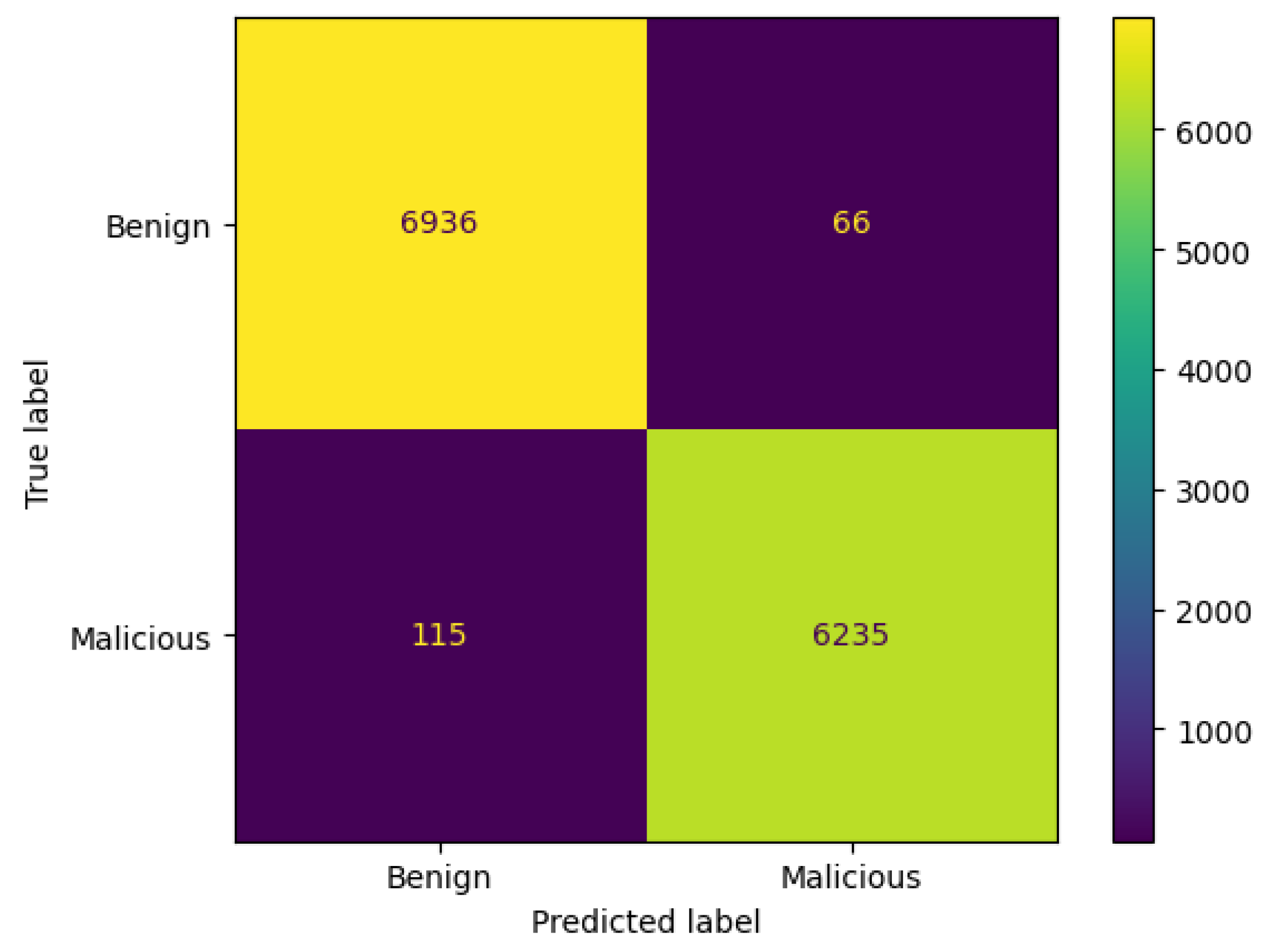
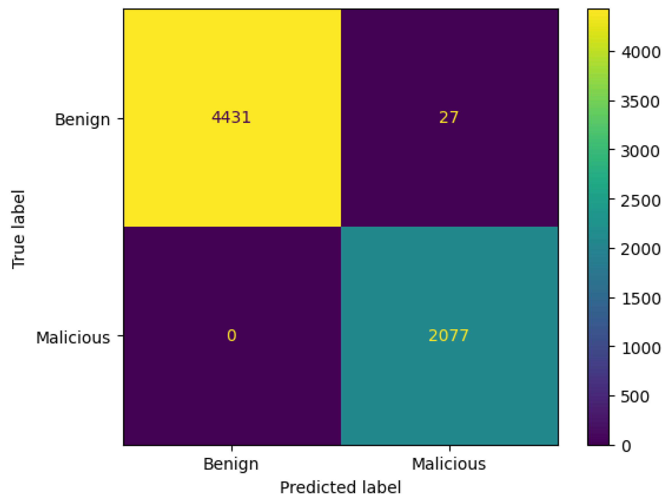
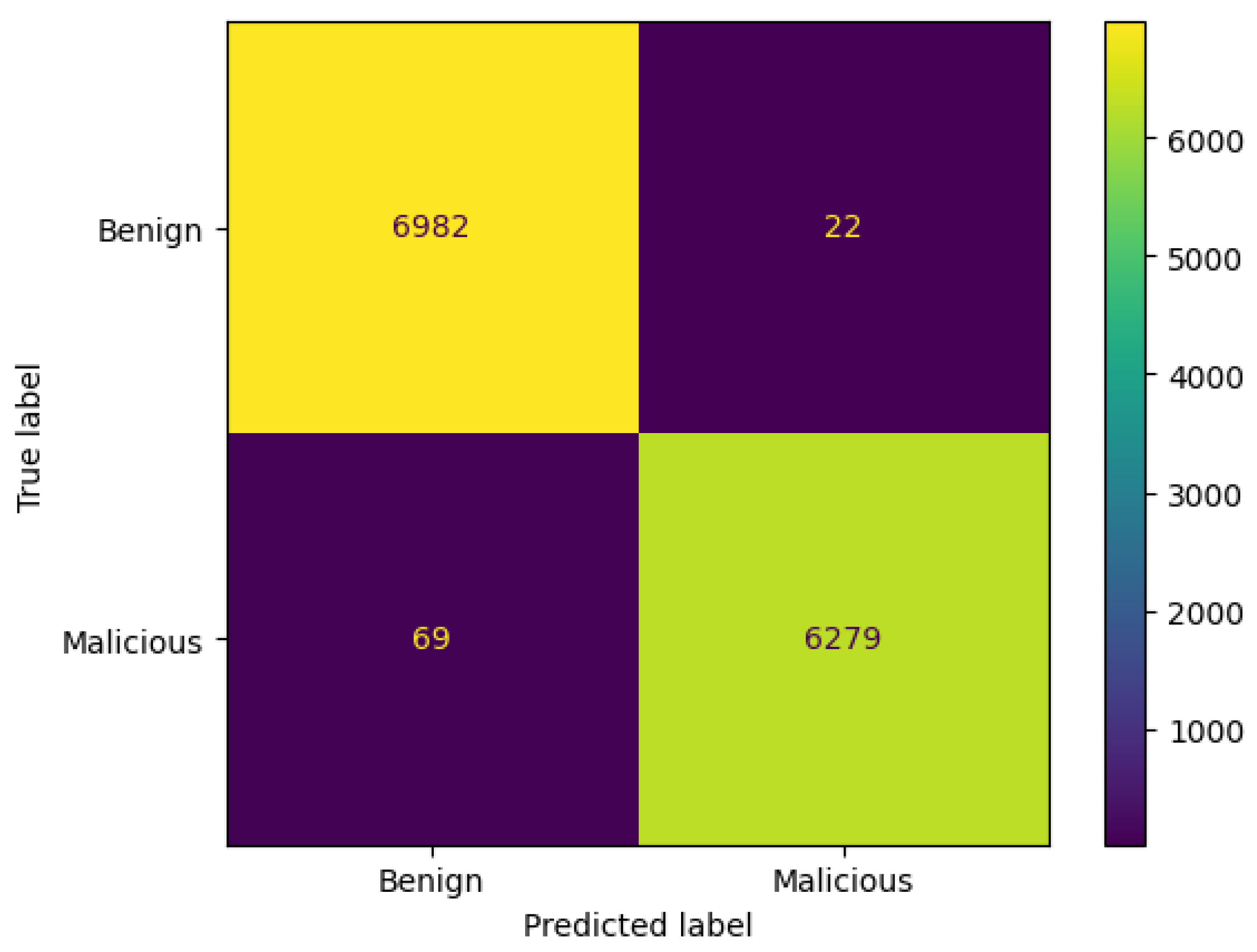
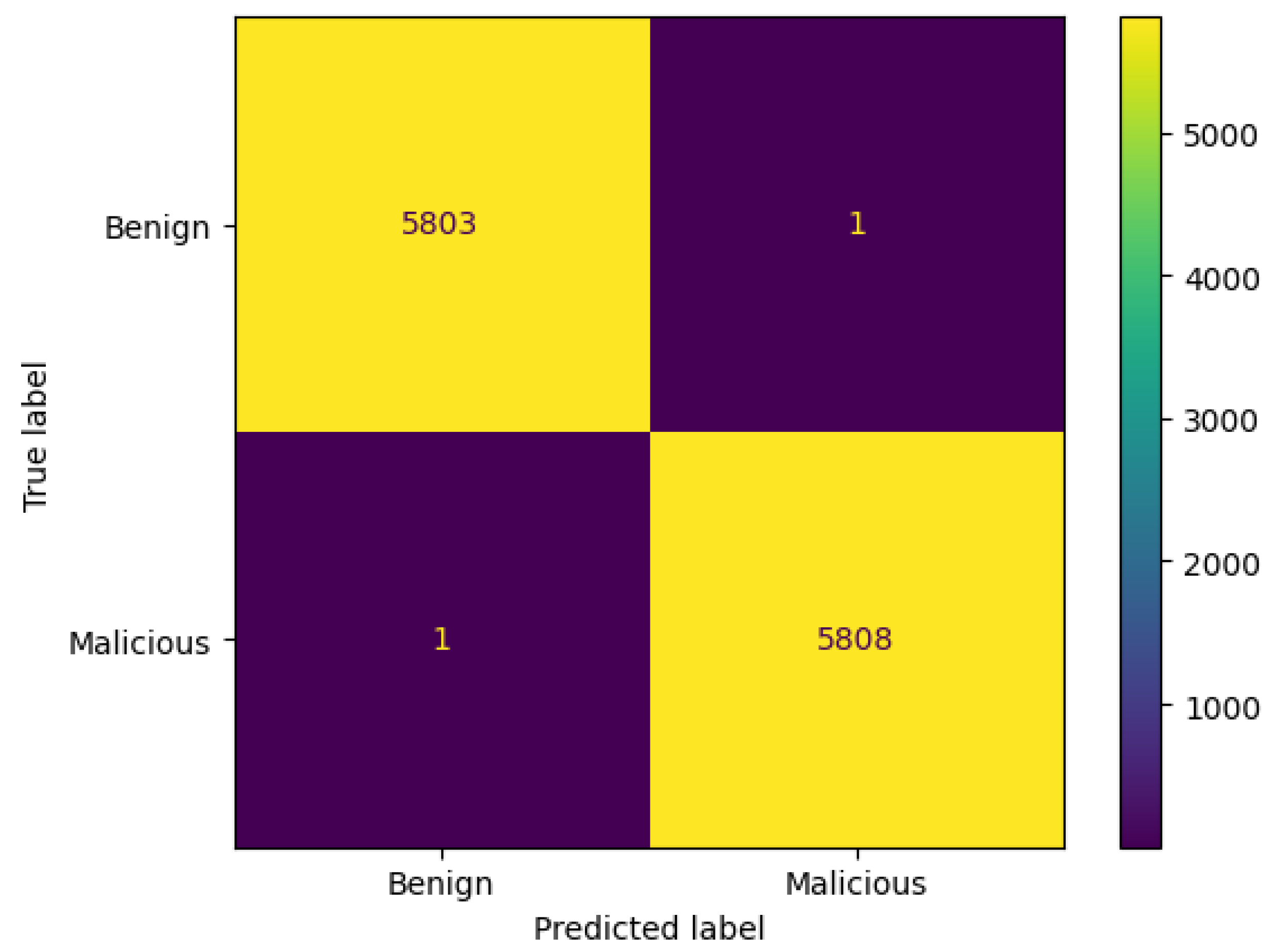
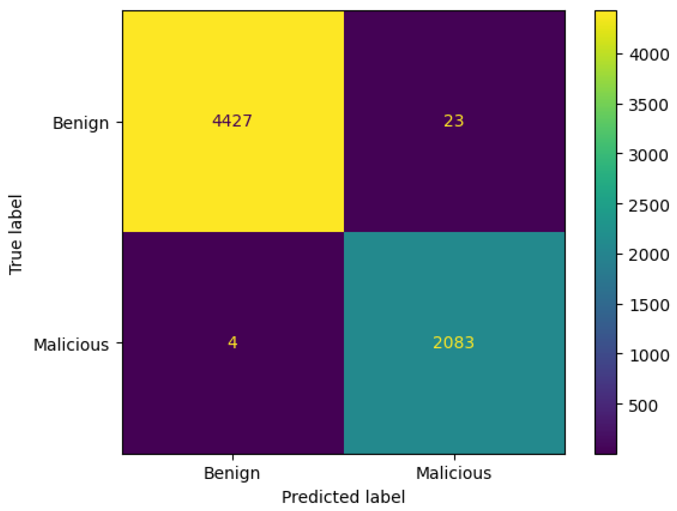
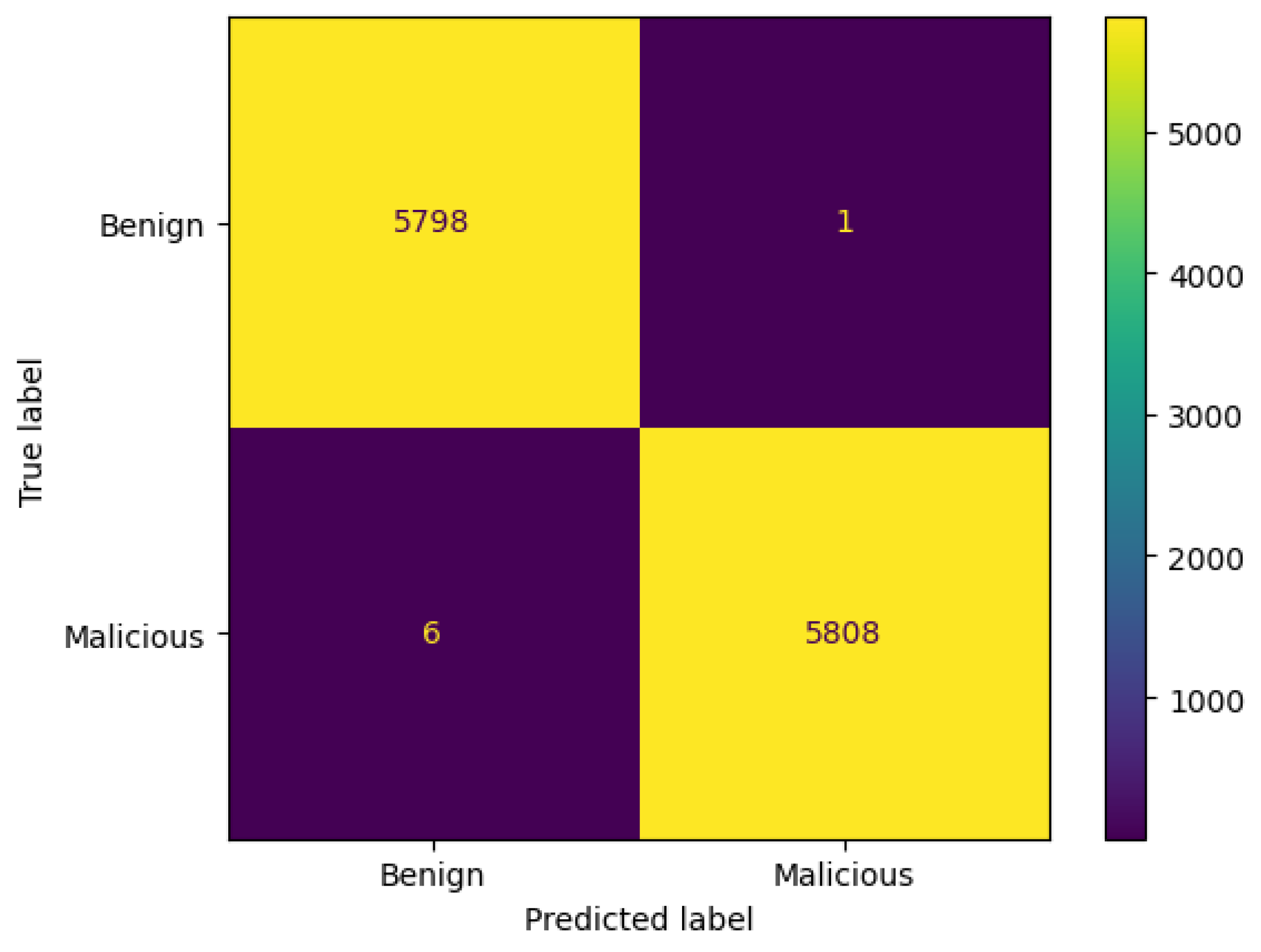
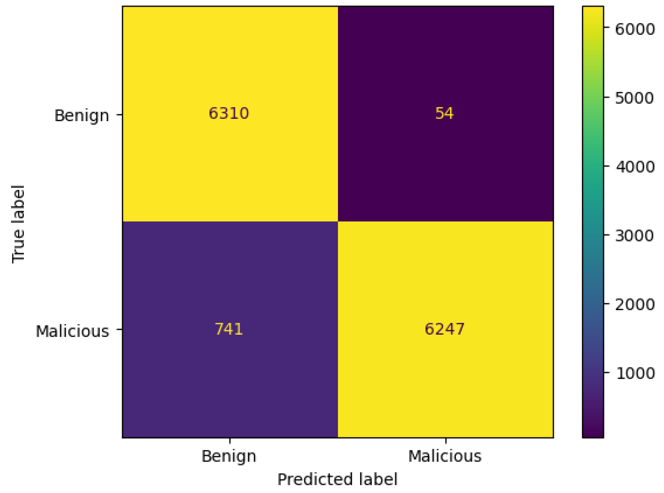
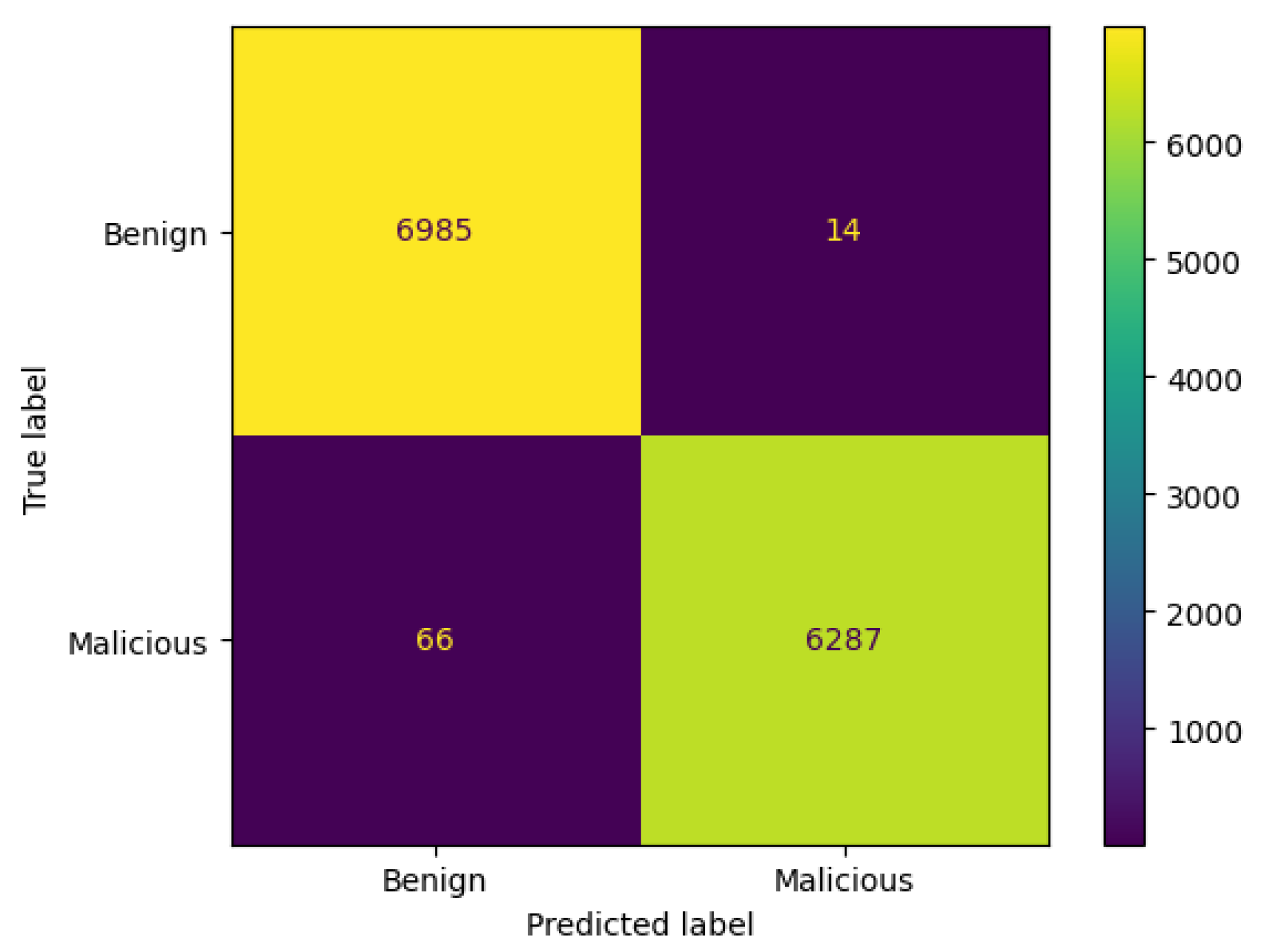
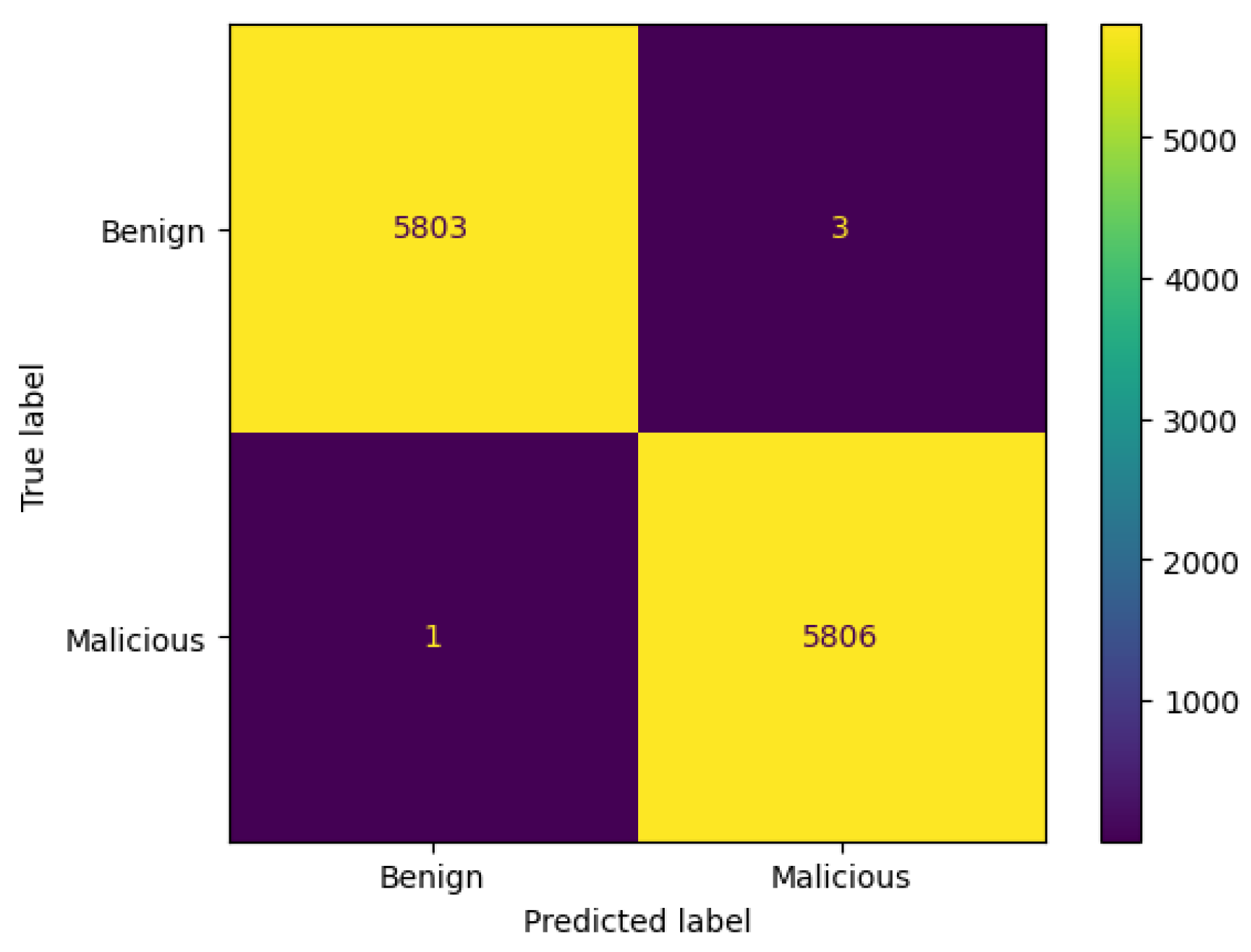
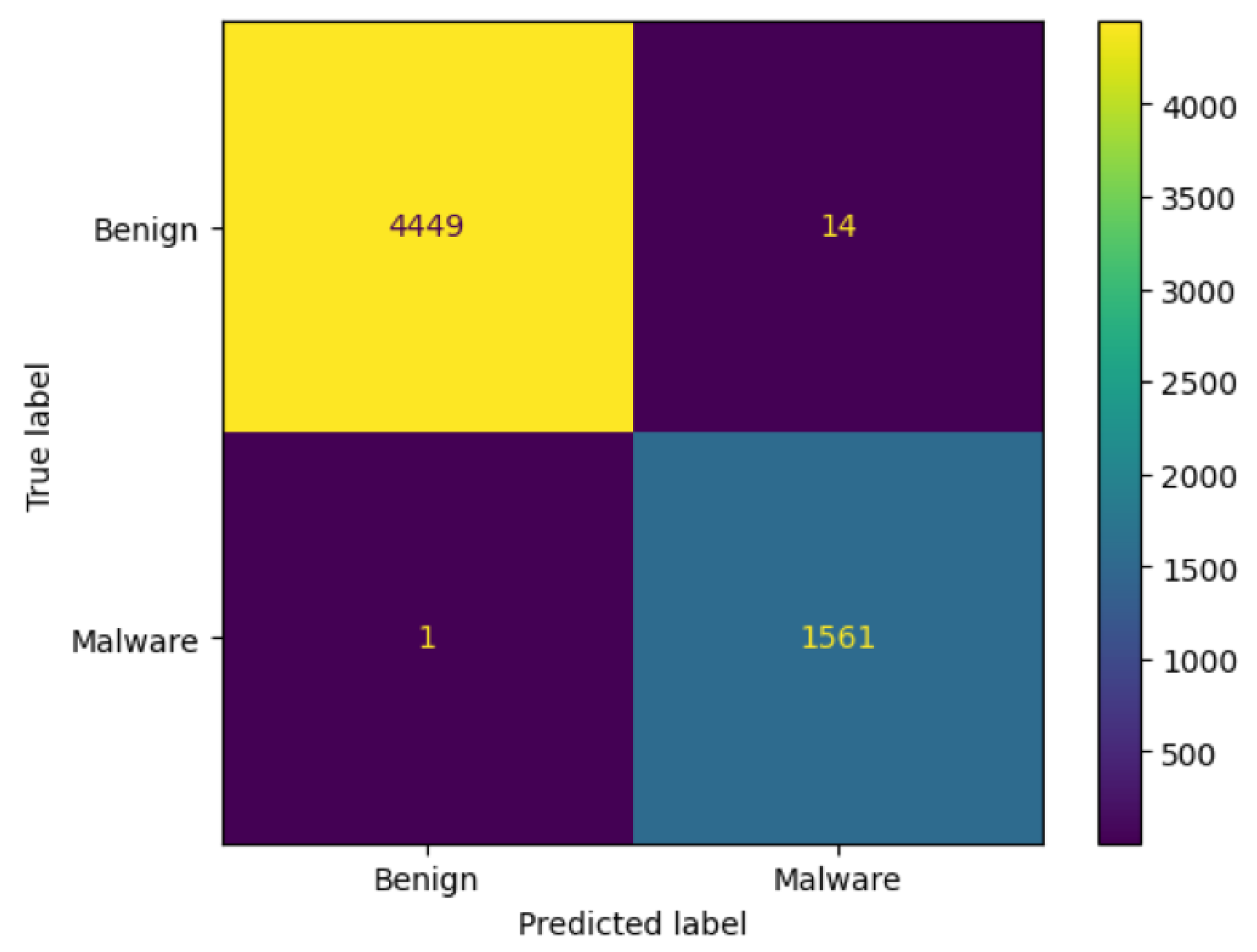
3.8.1. Confusion Matrix

Evaluating the performance of ML algorithms by using confusion matrices can provide significant insights into the performance and bias of different algorithms.

Table 7. Confusion matrix for binary classification.

Class/Prediction	Benign	Malicious
Benign	TN	FP
Malicious	FN	TP

presents the confusion matrix.

In order to determine the accuracy of the model or the correct rate, it is necessary to determine how accurate the model is for the given classification task.

$$Accuracy={\displaystyle \frac{TP+TN}{TP+TN+FP+FN}}$$

(2)

where the following apply:

• TN denotes correct prediction for the benign class.
• TP indicates correct prediction for the malicious class.
• FP implies incorrect prediction for the benign class. It is predicted as malicious, but it is actually benign.
• FN represents incorrect prediction for the malicious class. It is predicted as benign, but in reality, it is malicious.

According to the definition of precision, it is the ratio of true positives to all positives.

$$Precision={\displaystyle \frac{TP}{TP+FP}}$$

(3)

Recall can be defined as the ratio between the true positives and the sum of the false negatives plus the true positives.

$$Recall={\displaystyle \frac{TP}{TP+FN}}$$

(4)

F1-score indicates the degree of similarity between a predicted and true set based on the balance between precision and recall.

$$F1\text{-}Score=2\times {\displaystyle \frac{Precision\times Recall}{Precision+Recall}}={\displaystyle \frac{2TP}{2TP+FP+FN}}$$

(5)

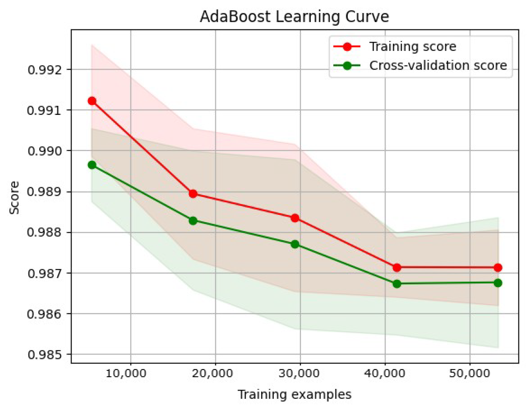
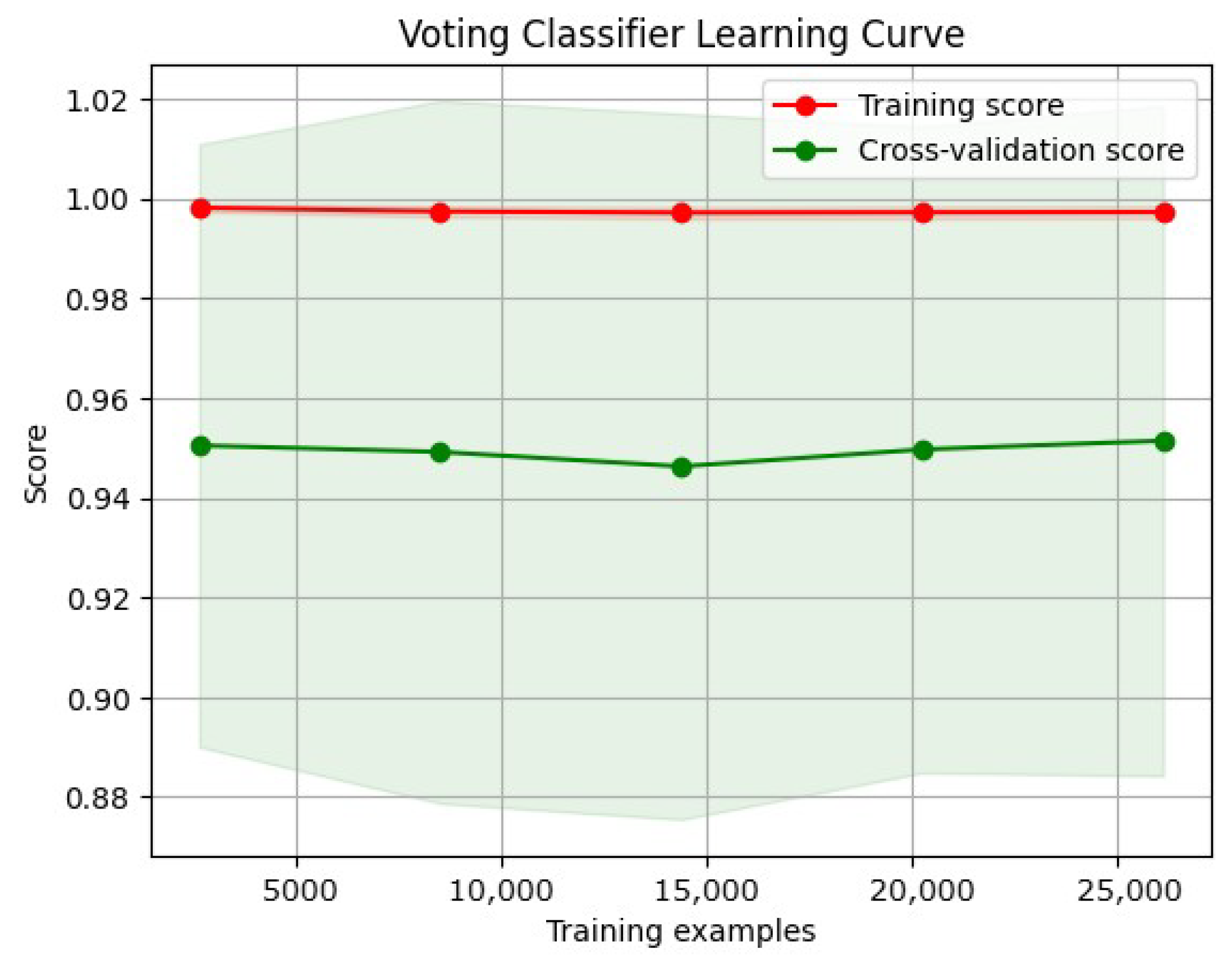
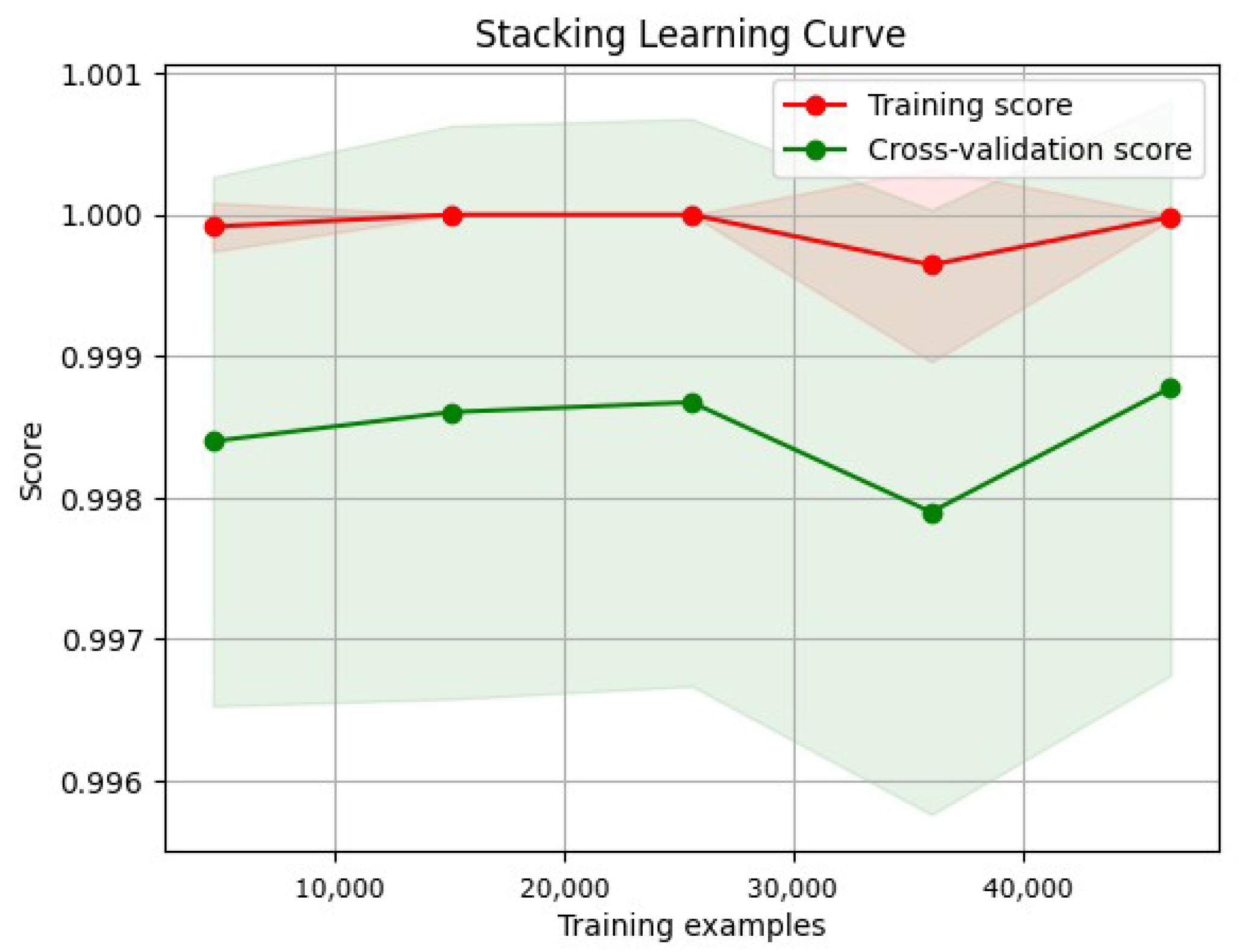
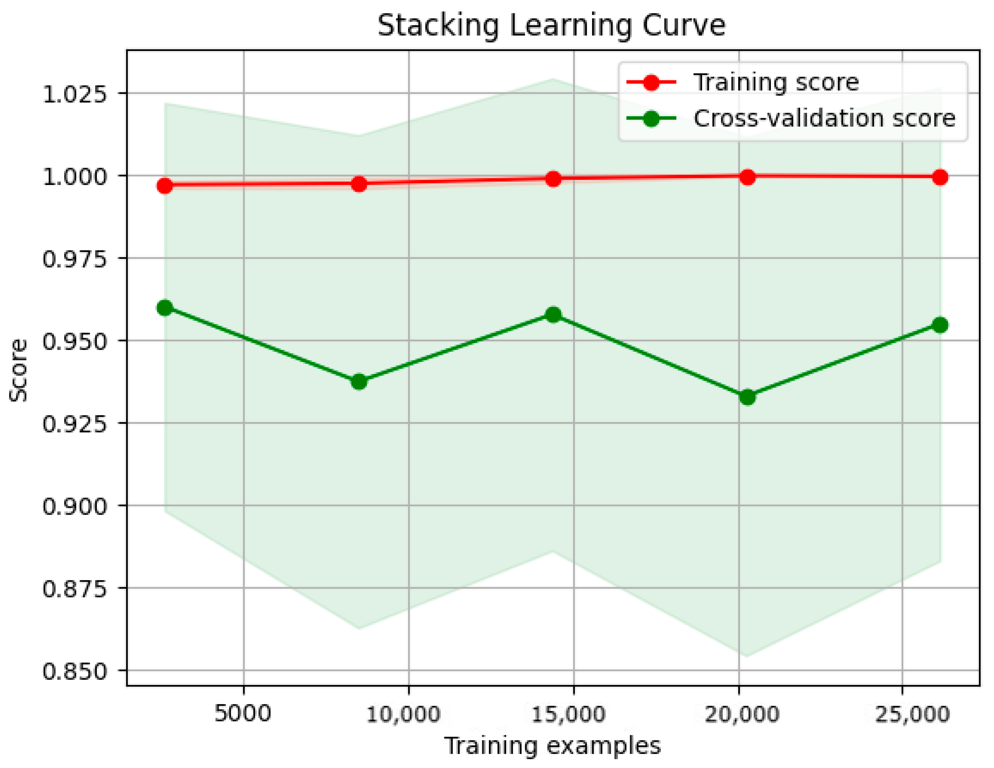
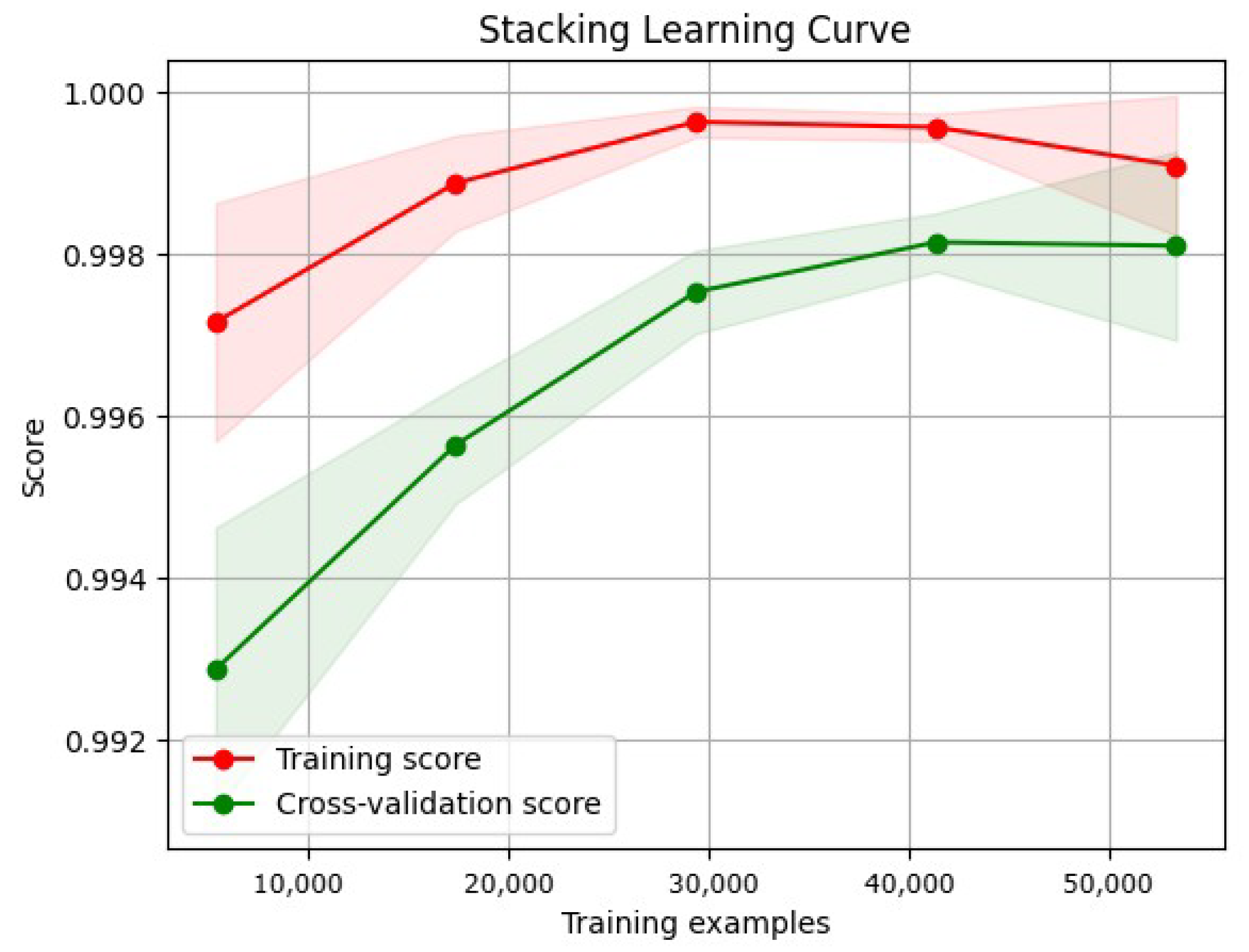
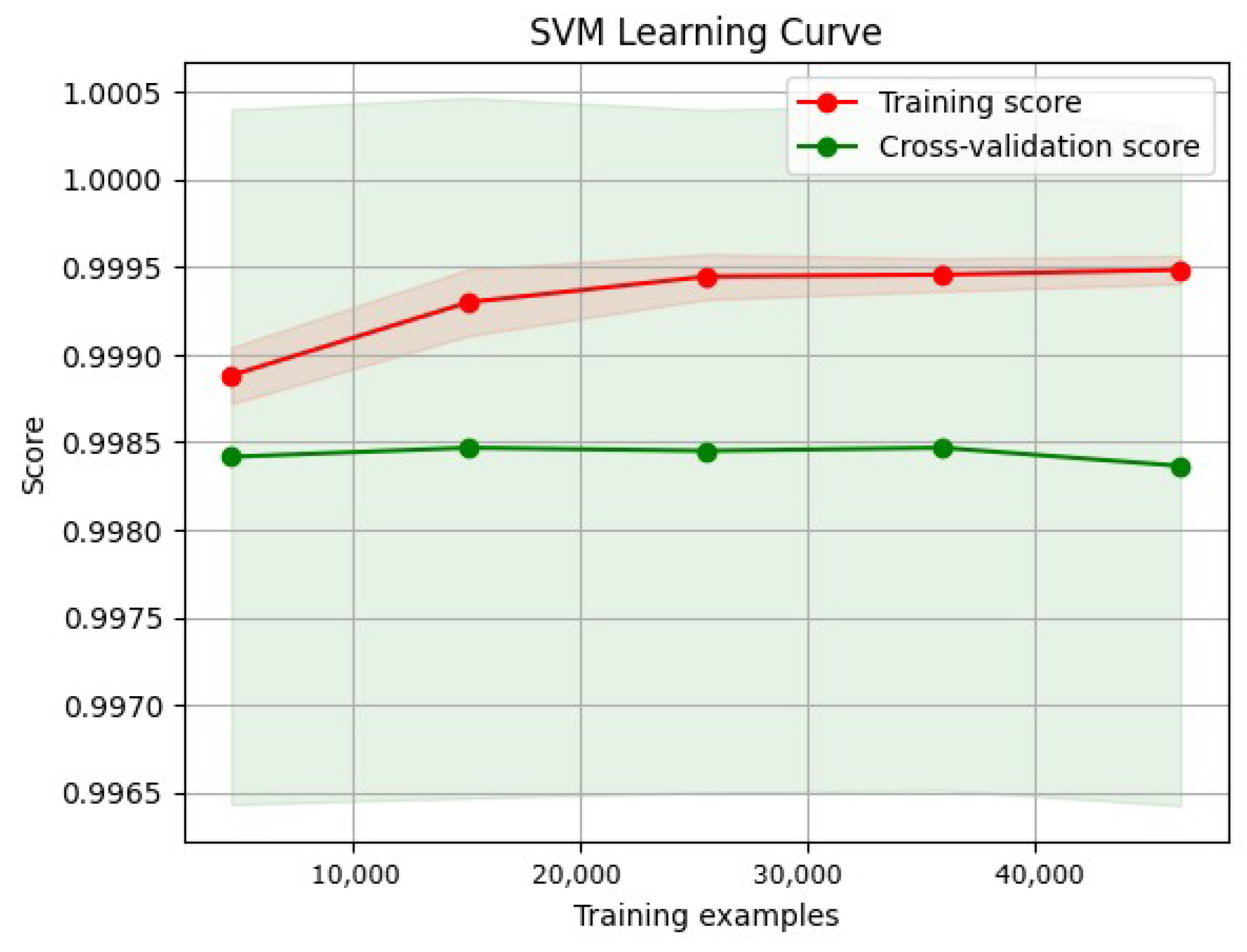
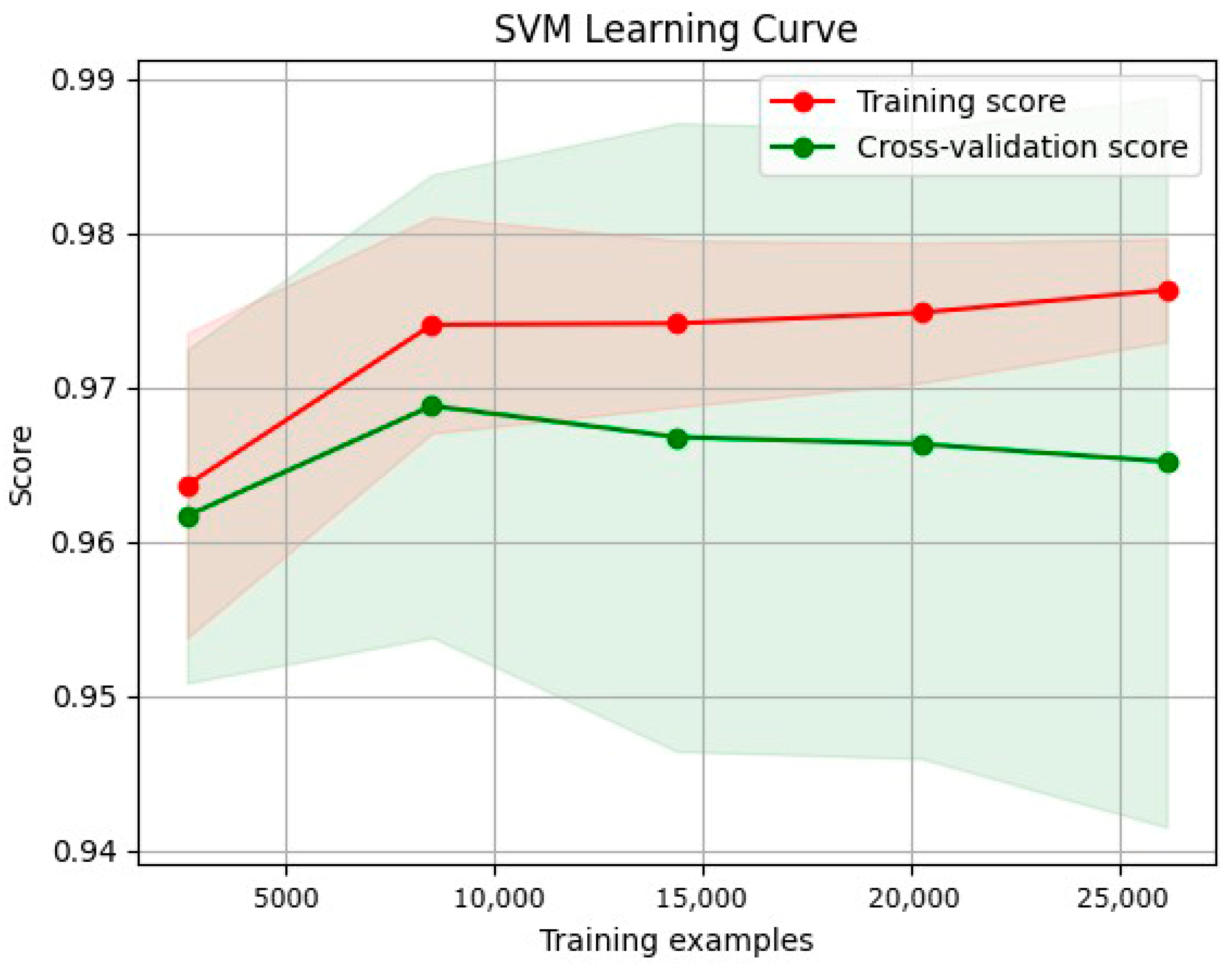
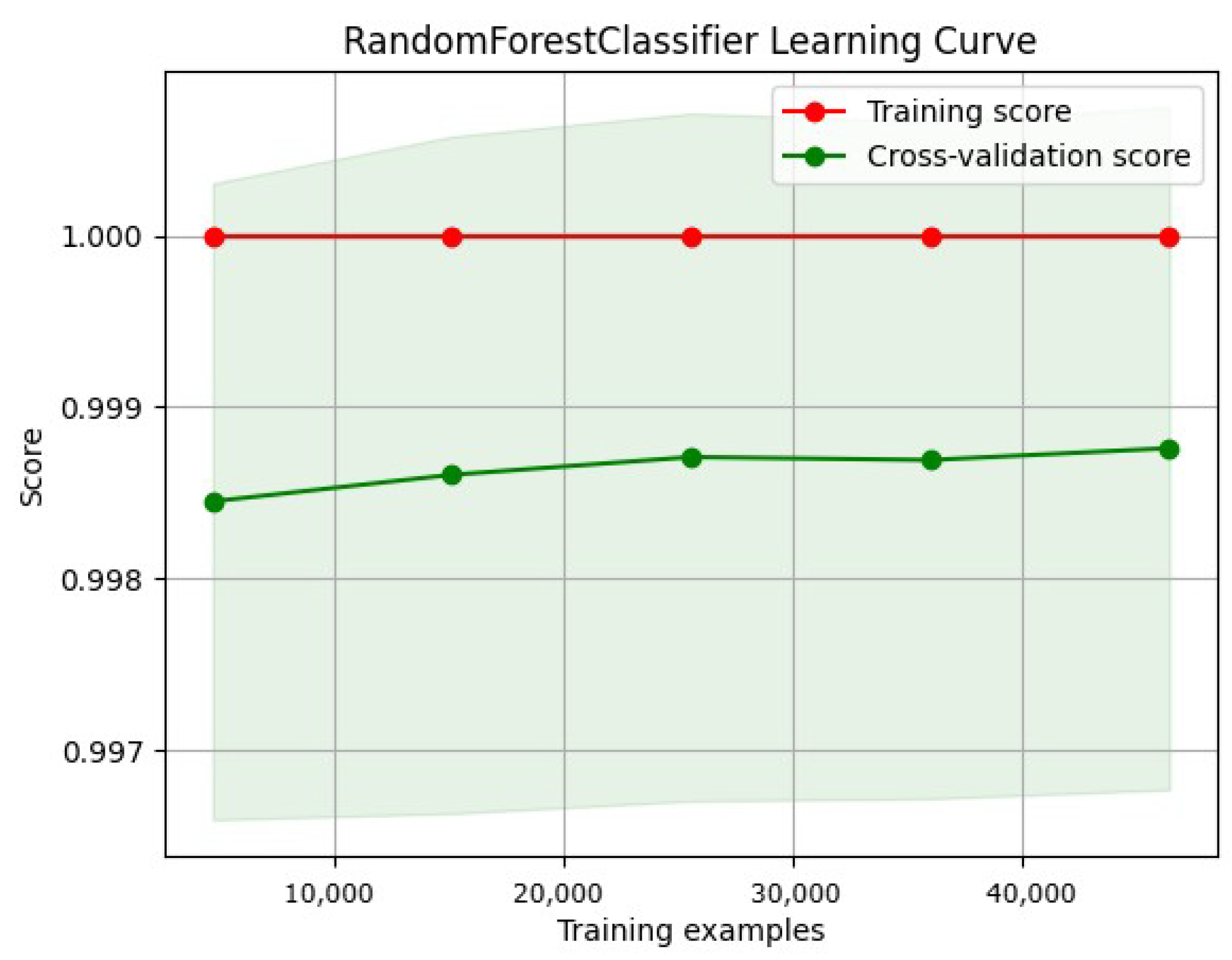
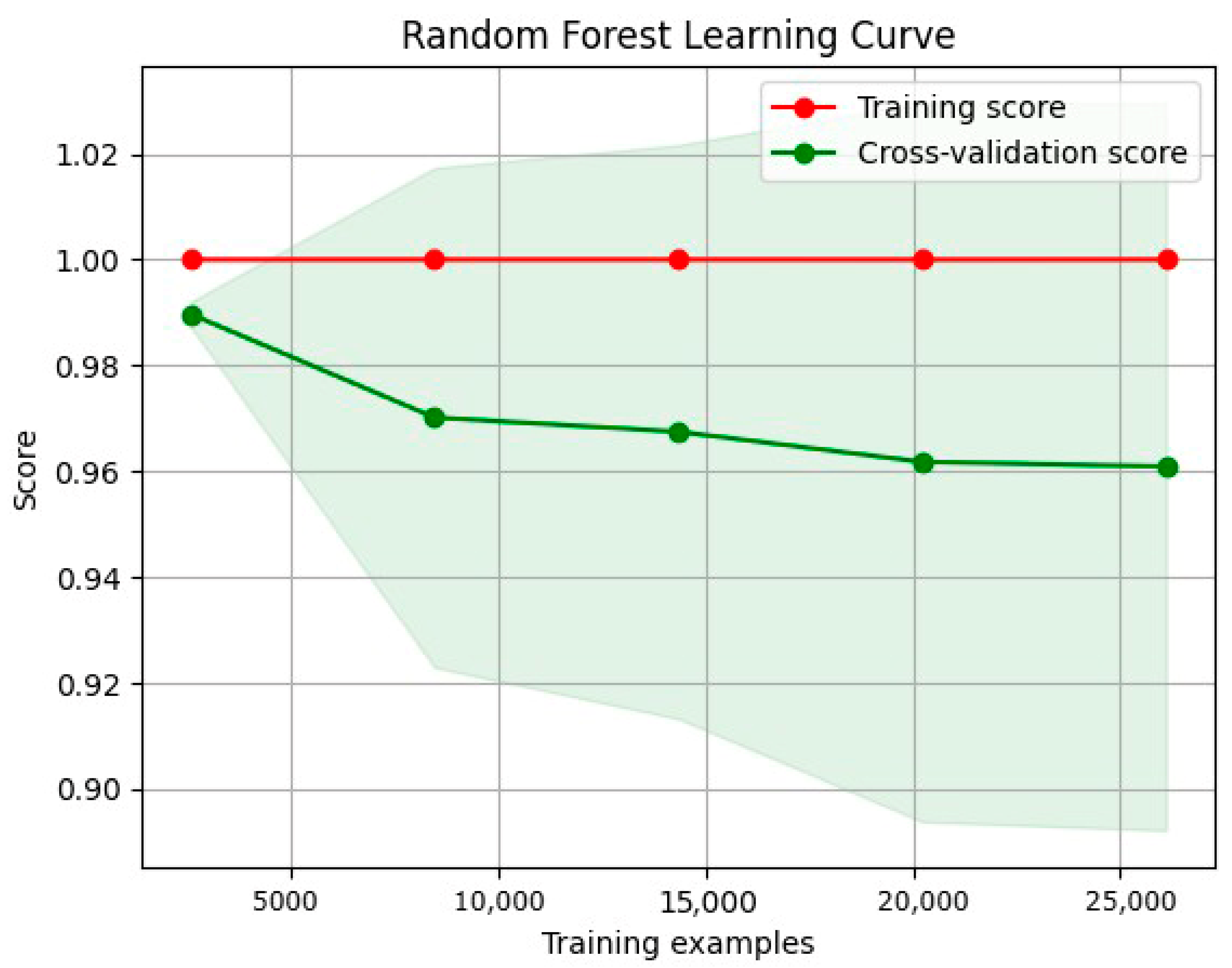
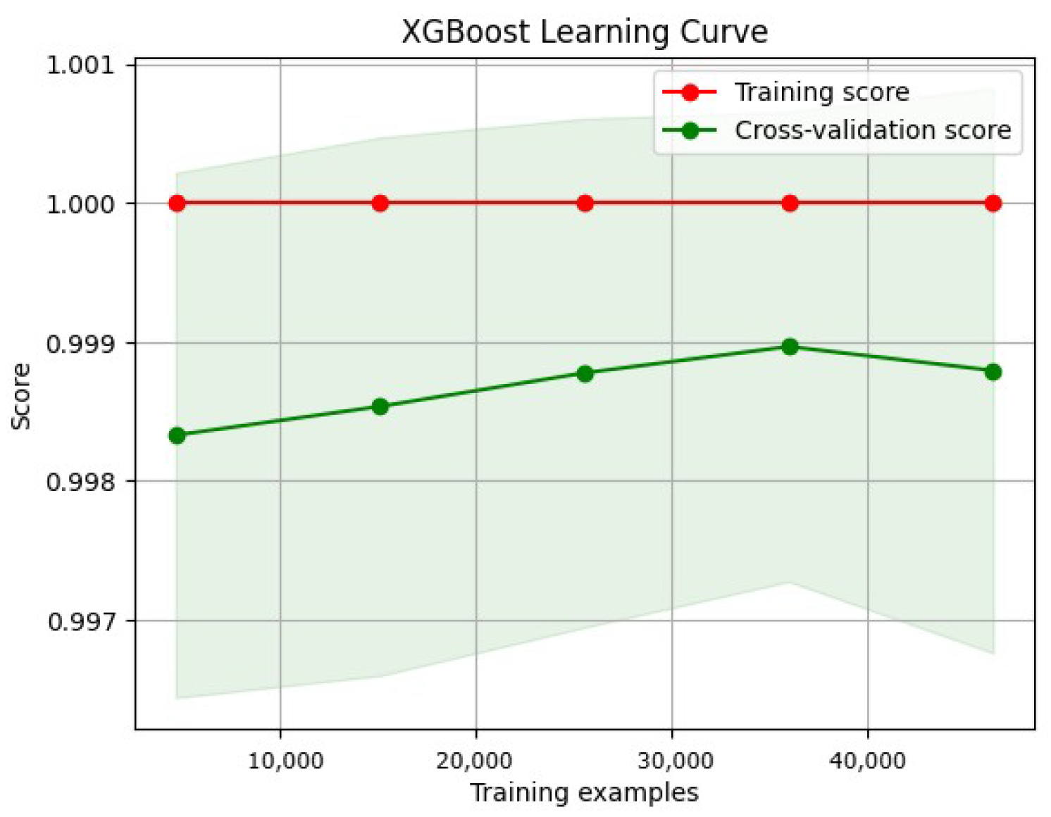
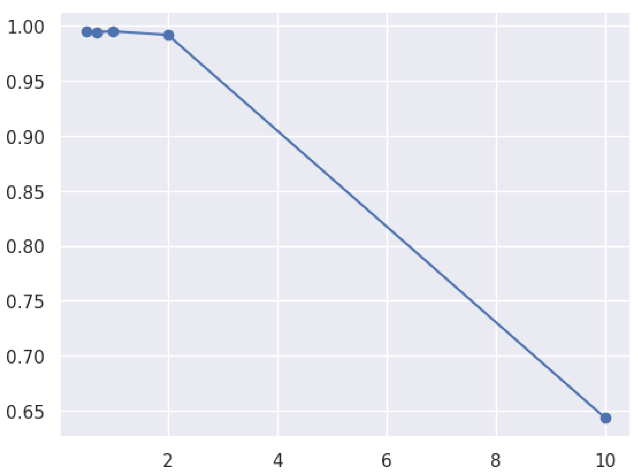
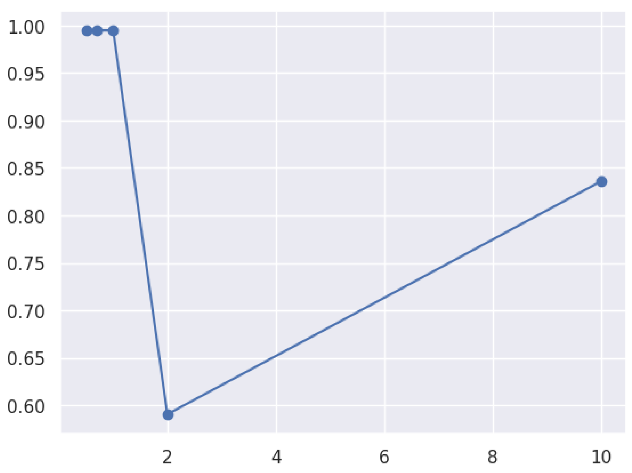
3.8.2. Learning Curve

ML uses learning curves to illustrate how a model’s performance correlates with training experience. A typical learning curve depicts the relationship between performance and experience [68]. Some of the most important characteristics can be summarized in the following [69]:

• Training curve: The training curve shows how the model performs on the training dataset as more training data are presented. Generally, as the model receives more training data, its performance on the training dataset will improve.
• Validation curves illustrate a model’s performance over various validation datasets. These curves can plateau or even worsen after a certain level, indicating that the model has become overfitted.
• Overfitting and underfitting:
  • An underfitted model has a high error rate during training and validation due to its oversimplistic nature, which makes it difficult to capture the underlying patterns in the data.
  • Overfitted models can learn that the training data contain noise. Consequently, the training error decreases, whereas the validation error increases.
• A low error rate across the training and validation curves is ideal for a model’s generalization to new datasets.

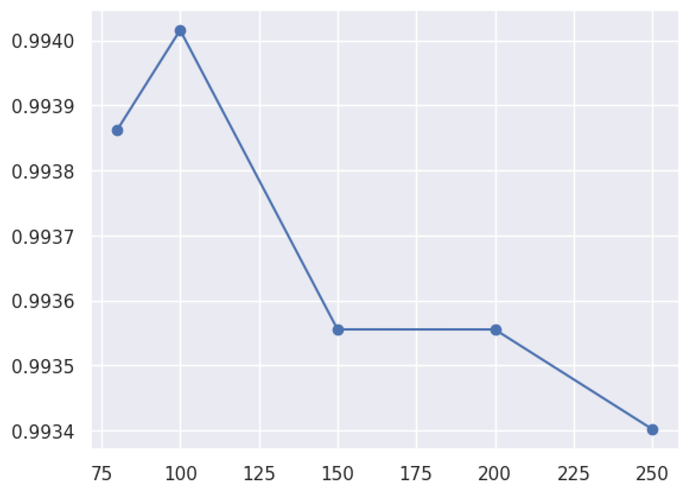
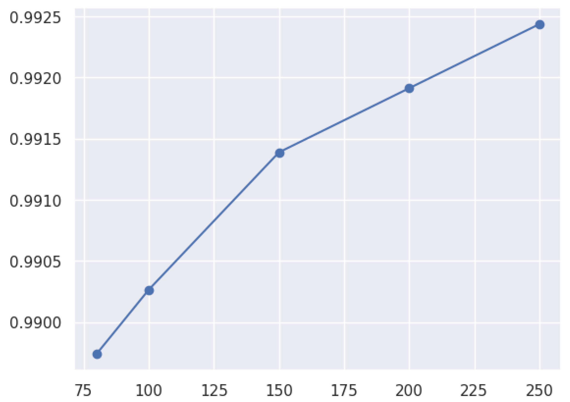
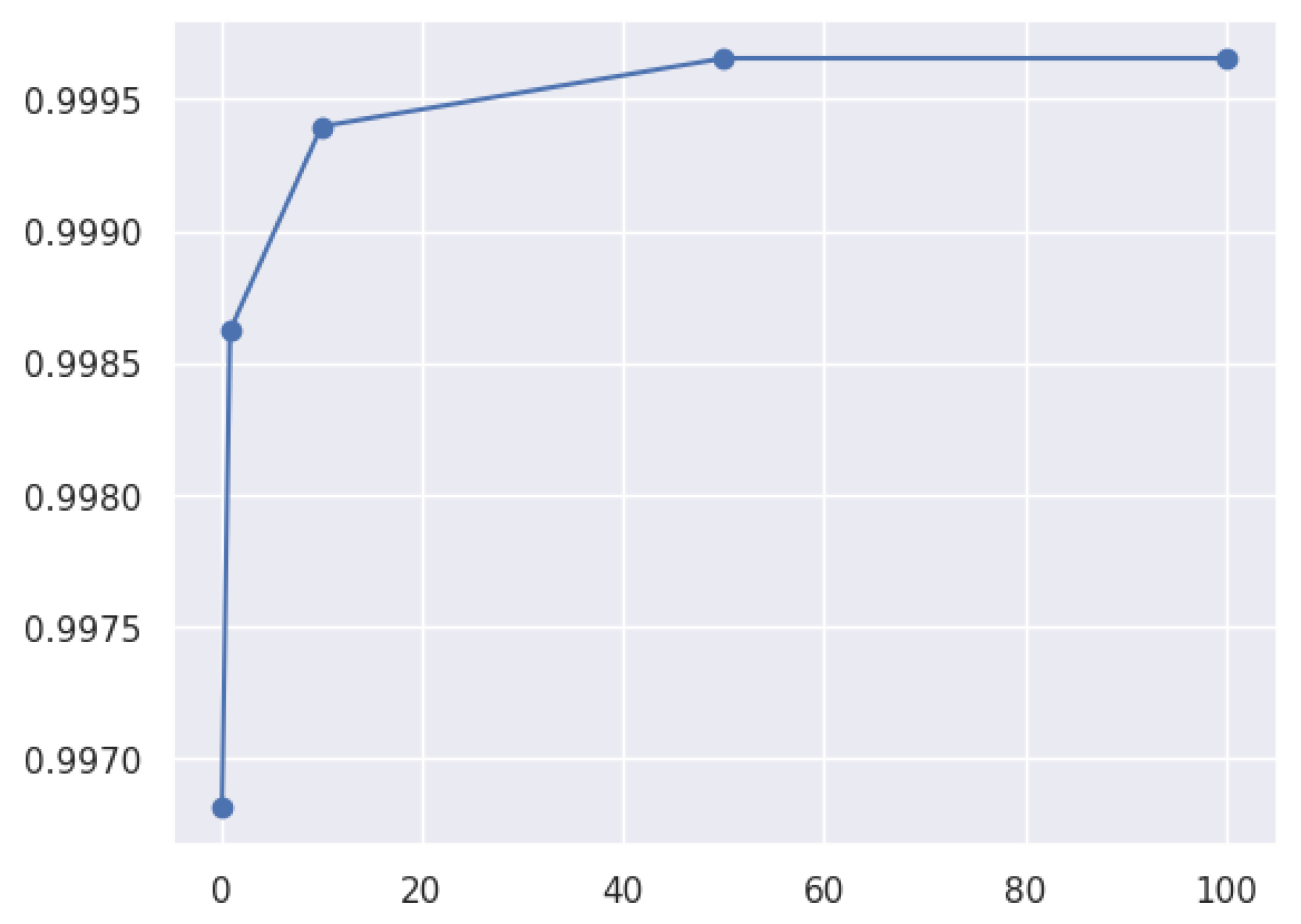
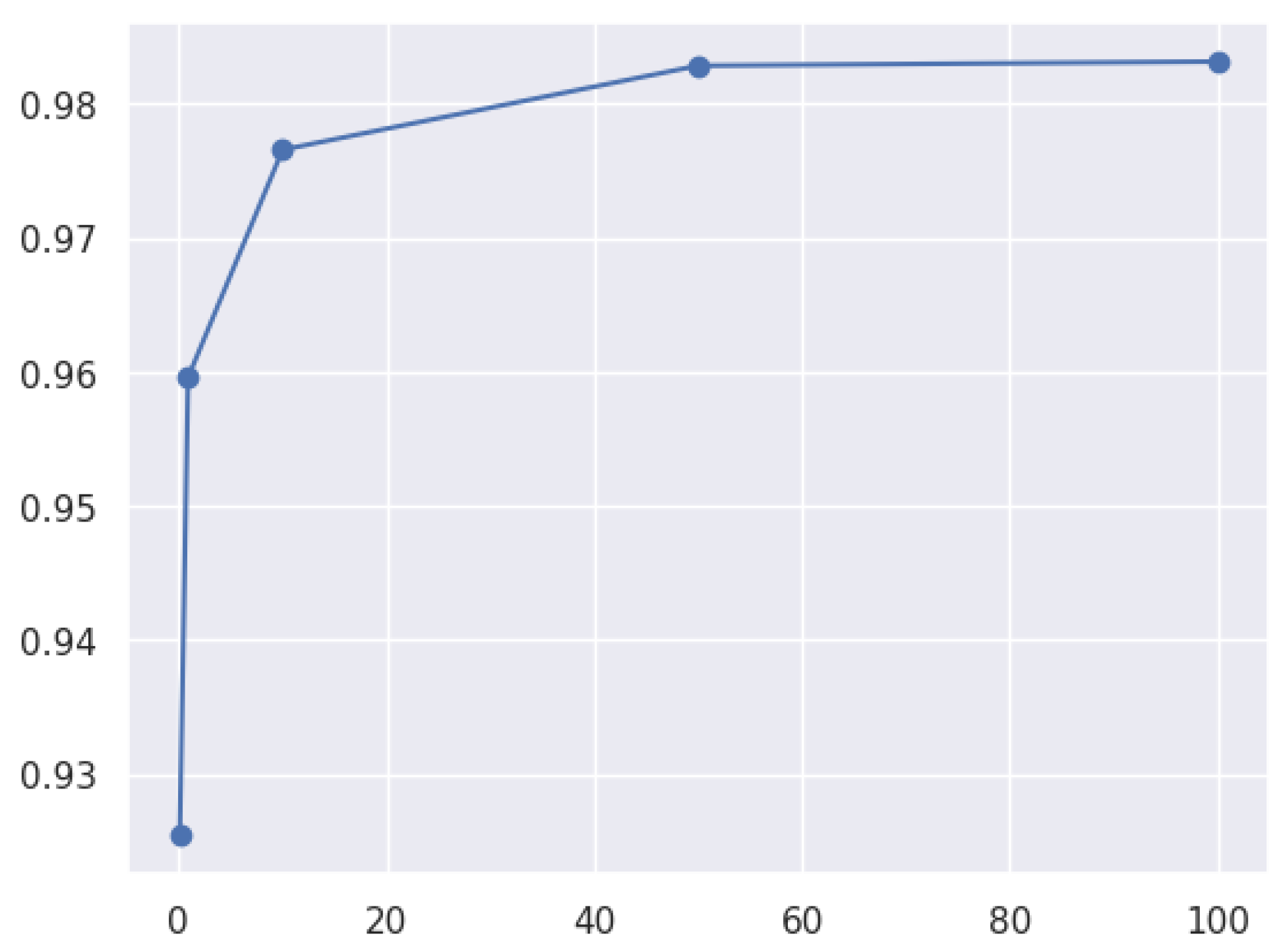
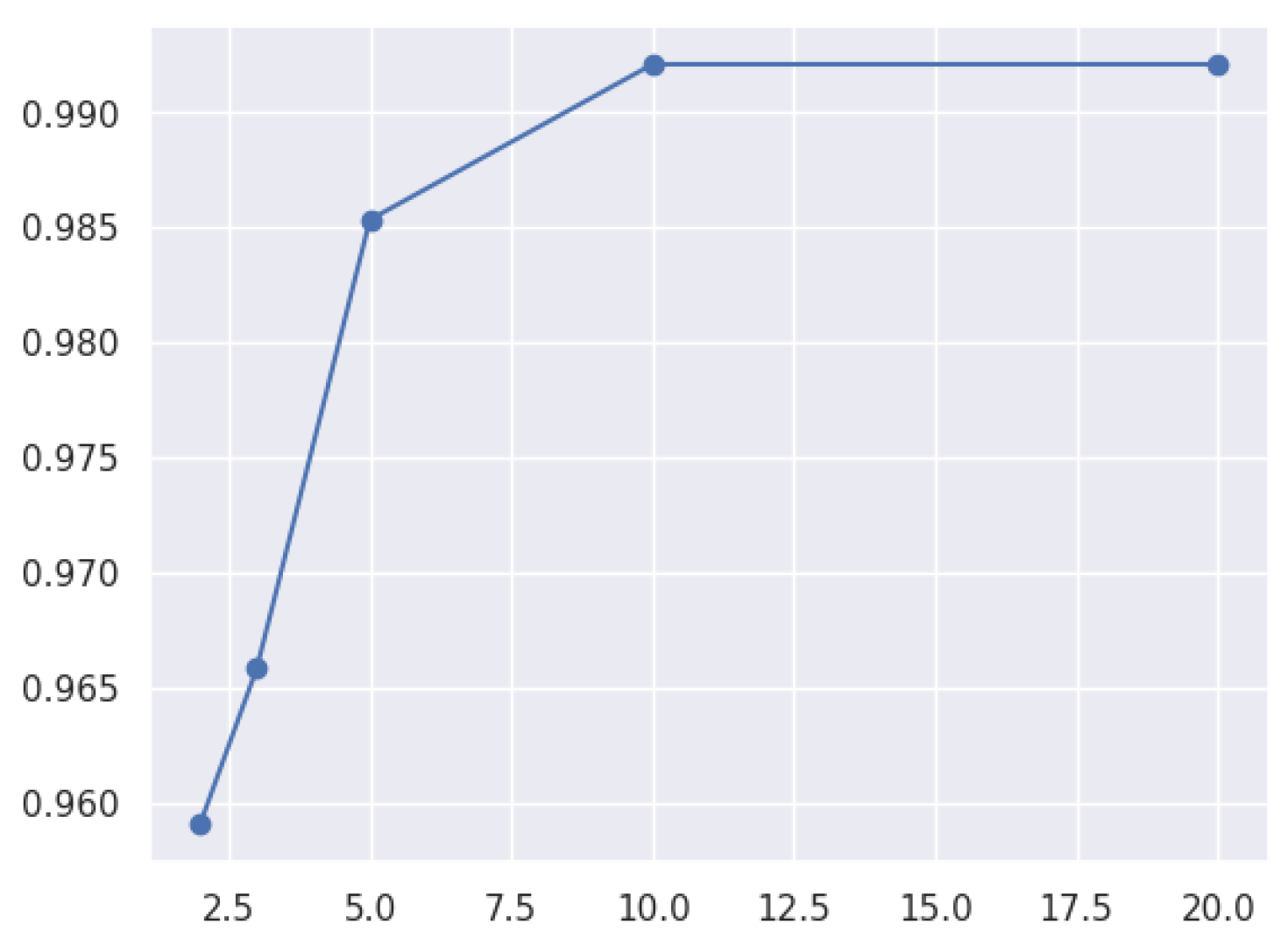
3.8.3. Hyperparameters in the Model

The risk of overfitting was reduced by tuning hyperparameters and using k-fold cross-validation. ML models perform better when hyperparameters are properly selected, since they influence an algorithm’s ability to fit the model to the data. In order to optimize the performance of the model, it is necessary to select appropriate hyperparameters. The hyperparameters of a model must be tuned to maximize its performance [70]. ML models are built by setting hyperparameters, which are settings that are not learned from data and are determined before training begins [71]. The following are critical components of hyperparameters [71]:

• The following types of hyperparameters can be identified:
  • Characteristics specific to a particular model may include the depth of decision trees (DTs) or the number of hidden layers within a neural network, for example.
  • Training-specific factors include the learning rate or batch size in gradient descent.
• A hyperparameter tuning approach involves finding the best parameters to optimize a model’s performance on a given task. It can be carried out through grid search, Bayesian optimization, or random search.
• In terms of importance, the following apply:
  • Optimizing hyperparameters can significantly improve a model’s performance.
  • Controlling overfitting and underfitting can be achieved by altering hyperparameters, such as the regularization parameter.
• The challenge of tuning hyperparameters can be computationally expensive and time-consuming, especially for models with a large number of parameters and complex interactions among them.

With GridSearchCV, tuning hyperparameters in ML efficiently and effectively is possible. A systematic evaluation of hyperparameters creates a grid of possible combinations. Combinations that perform best are evaluated by using cross-validation and selected according to performance. In this way, hyperparameter tuning can be automated, improving model performance and reducing the need for manual trial and error [70].

A description of each hyperparameter and its values is provided in

Table 8. Hyperparameter and tuning values for each ML algorithm.

ML Algorithm	Hyperparameter	Values
AdaBoost	n_estimators	80, 100, 150, 200, 250
Voting	voting	Hard, soft
Stacking	passthrough	True, False
SVM	Regularization parameter (C)	0.1, 0.9, 10.0, 50.0, 100.0
RF	max_depth	2, 3, 5, 10, 20
XGBoost	Learning rate	0.5, 0.7, 1, 2, 10

. In addition, k-fold cross-validation can enhance the model’s robustness and generalizability when used during the evaluation process. To train the model, k = 5 subsets of the datasets were divided into one set, and the model was trained on the sets of data. By repeating this procedure five times, the cross-validation performance metrics for each fold were obtained. In addition, the results of the cross-validation process are not discussed in detail in this study.

4. Results and Discussion

This experiment was conducted on an HP laptop with an Intel(R) Core(TM) i7-8550U processor @ 1.80 GHz and 2.00 GHz, with 16.0 GB RAM, and Windows 11. An IDS was developed by using ML techniques on the open-source Google Colab Notebook platform. This section will present and analyze the results.

4.1. Results

4.1.1. AdaBoost

This model was trained on the first dataset, CIC-MalMem-2022, with an accuracy of 99.94%. Based on the confusion matrix shown in Figure 3, the model correctly predicted 5805 malicious and 5802 benign instances. However, two malicious instances were incorrectly predicted as benign, and four benign instances were incorrectly predicted as malicious. For CIC-IDS-2018, the accuracy was 99.11%, and the confusion matrix in Figure 4 indicates that the model correctly predicted 2059 malicious instances and 4418 benign instances. Nevertheless, 13 malicious instances were incorrectly predicted as benign, and 45 benign instances were incorrectly predicted as malicious. CIC-IDS-2017 had an accuracy rate of 98.64%, and the confusion matrix in Figure 5 shows that the model accurately predicted 6235 malicious instances and 6936 benign instances. However, 115 malicious instances were incorrectly predicted as benign, while 66 benign instances were incorrectly predicted as malicious. The learning curve for the CIC-MalMem-2022 dataset is depicted in Figure 6, which shows that the training score is 100% accurate in every rotation; however, cross-validation scores show different accuracy levels in each cycle. The cross-validation score starts at 99.82%, reaches 99.88% with training examples ranging from 20,000 to 30,000, and then continues with an accuracy of 99.86%. These training and validation percentage results indicate no evidence that overfitting has occurred. Figure 7 presents the learning curve for the CIC-IDS-2018 dataset, which shows that the training scores have an accuracy of around 99.99% in every cycle, but cross-validation scores range from 94% to 96%. By comparing the results of training and cross-validation, it is apparent that the model is balanced. In Figure 8, the learning curve for the CIC-IDS-2017 dataset indicates that the model performs well in both training and cross-validation, as demonstrated by the high scores in both training and cross-validation. There is a slight difference in training and cross-validation scores, which is a typical pattern. Thus, the model does not overfit the training data. The effective hyperparameter for the AdaBoost model is n_estimators. Five values are assigned to check the best n_estimators, and they are 80, 100, 150, 200, and 250; for the experiment on the CIC-MalMem-2022 dataset, the best value is 80, with a time of 0.102 s; moreover, all values yield 100% accuracy, as shown in Figure 9; so, in this case, it is necessary to check the time. For the CIC-IDS-2018 dataset, the best parameter is 100, with a mean test score of 99.40% and a mean test time of 0.191 s. Figure 10 illustrates the relationship between n_estimators and their accuracy. According to Figure 11, the best parameter for the CIC-IDS-2017 dataset is 250. The mean test score and mean test time for the CIC-IDS-2017 dataset are 99.24% and 0.358 s, respectively.

4.1.2. Voting Classifier

Based on the first dataset, CIC-MalMem-2022, the model was trained and had an accuracy result of 99.96%. According to the confusion matrix in Figure 12, the model correctly predicted 5806 malicious and 5803 benign instances. However, one malicious instance was incorrectly predicted as benign, and three benign instances were incorrectly predicted as malicious. The accuracy result for the CIC-IDS-2018 dataset is 99.58%, and based on Figure 13, the model correctly predicted 2077 malicious instances and 4431 benign instances. In addition, 27 benign instances were incorrectly predicted as malicious, while no malicious instances were incorrectly predicted as benign. The accuracy result for the CIC-IDS-2017 dataset is 99.31% for this model, and the confusion matrix in Figure 14 indicates that the model correctly predicted 6279 malicious and 6982 benign instances. This model made incorrect predictions regarding 69 malicious instances and 22 benign instances. The learning curve for the CIC-MalMem-2022 dataset in Figure 15 indicates that the training score is 100% accurate in each cycle, meaning that the model is well trained to handle the data. In contrast, cross-validation scores are accurate between 99.80% and 99.90%, demonstrating the model’s ability to identify and learn new datasets. Compared with the cross-validation score, which ranges from 94% to 96%, the CIC-IDS-2018 dataset’s training scores achieved 99.99% accuracy in every cycle, as shown in Figure 16. With more examples of data, a classifier learns more about the data, and as the number of training examples increases, the cross-validation score also increases at a slower rate. For the CIC-IDS-2017 dataset, as shown in Figure 17, the training score starts at 99.51% and then drops to 99.46%, while the cross-validation score starts at 99.30% and then decreases to about 99.28% in accuracy. As a result of its effectiveness in learning, the Voting classifier will likely generalize well to new data. There are two options for the voting hyperparameter in the Voting model: hard or soft. The hard option is based on a majority vote, while the soft option is based on the average probability. In the CIC-MalMem-2022 dataset, the soft parameters were found to be the most effective, with a mean test score of 99.90% and a mean score time of 0.38 s. On the other hand, the hard option results in a mean test score of 99.88%, and the mean test time is 0.76 s. Moreover, the best parameter for the CIC-IDS-2018 dataset is also the soft value, with a mean test score of 99.44% and a mean score time of 0.22 s. Furthermore, the best parameter value for the CIC-IDS-2017 dataset is also soft, with a 99.39% mean test score and a 0.78 s mean test time.

4.1.3. Stacking Classifier

In this model, the accuracy result for the CIC-MalMem-2022 dataset was 99.98%. According to the confusion matrix in Figure 18, the model correctly predicted 5808 malicious and 5803 benign instances. However, one malicious instance and one benign instance were incorrectly predicted. In the CIC-IDS-2018 dataset, the model achieved a 99.61% accuracy, and per the confusion matrix in Figure 19, 2083 malicious instances were correctly predicted, whereas 4427 benign instances were correctly predicted. However, the model predicted 4 malicious instances as benign and 23 benign instances as malicious. For the CIC-IDS-2017 dataset, the accuracy rate was 99.86%, and based on the confusion matrix in Figure 20, the model predicted only two malicious samples as benign. Figure 21 indicates the learning curve for the CIC-MalMem-2022 dataset. According to Figure 21, the training score increases as the number of training examples increases. As the model receives more examples of the data, it becomes more knowledgeable about the data. As a result, the cross-validation score also increases, indicating that the model does not overfit the training data. In this case, a good sign is that the model learns the data effectively and can also generalize to new data. The Stacking learning curve in Figure 22 for the CIC-IDS-2018 dataset shows that the training and cross-validation scores increase as the number of training examples increases. By seeing more examples, the Stacking model can better understand the data; the cross-validation score eventually plateaus around 95.51%, whereas the training score continues to increase, reaching 100%. The CIC-IDS-2017 learning curve in Figure 23 shows that the training score increases with the increase in the number of training examples and cross-validation. A training score of 99.66% is achieved and continues to increase, reaching 99.85%; a cross-validation score of 99.25% is achieved and continues to increase, reaching get 99.81%. This model’s passthrough hyperparameter can be set to “True” or “False”. In the CIC-MalMem-2022 dataset, the best parameter is “True”, with a mean test score of 99.94% and a mean test time of 0.640 s. The best parameter for the CIC-IDS-2018 dataset is “False”, with a mean test score of 99.38% and a mean test time of 0.45 s. The best parameter value for the CIC-IDS-2017 dataset is “True”, with a mean test score of 99.30% and a mean test time of 0.414534 s.

4.1.4. SVM

This model achieved a 99.93% accuracy rate on the CIC-MalMem-2022 dataset. According to Figure 24, the model correctly predicted 5808 malicious instances and 5798 benign instances. However, one malicious instance was incorrectly predicted as benign, and six benign instances were incorrectly predicted as malicious. For the CIC-IDS-2018 dataset, the accuracy result was 97.41%. Based on Figure 25, the confusion matrix shows that the model correctly predicted 1976 malicious and 4390 benign instances. However, 41 malicious instances were incorrectly predicted to be benign, and 128 benign instances were incorrectly predicted as malicious. In the CIC-IDS-2017 dataset, accuracy was achieved at 94.04% by this model, and the confusion matrix in Figure 26 indicates that the model incorrectly predicted 741 malicious samples as benign and 54 benign samples as malicious. For the CIC-MalMem-2022 dataset, the learning curve, as shown in Figure 27, indicates that as the number of training examples increases, the training score rises. The training score starts at 99.88%, a little higher than the cross-validation score, which begins at 99.84% accuracy; however, the cross-validation score decreases after 40,000 samples. As shown in Figure 28, the training and cross-validation scores for the CIC-IDS-2018 dataset increase with the increase in training examples. Nevertheless, the cross-validation score plateaus after a certain point, whereas the training score continues to increase. The learning curve for the CIC-IDS-2017 dataset in Figure 29 indicates that the training score increases with the number of training examples because the classifier becomes more proficient at analyzing the data as more samples are viewed. However, the cross-validation score plateaus after a certain number of examples. This results in the classifier needing help to learn from the data, and the additional training examples do not improve the classifier’s performance. For the SVM model, the regularization parameter (C) is a very important parameter. As the value of the parameter increases, the classification accuracy improves (or the regression error is reduced); however, overfitting may also occur. In this model, five different values were assigned to C: 0.1, 0.9, 10.0, 50.0, and 100.0. As shown in Figure 30, the best parameter was 50.0 for the CIC-MalMem-2022 dataset. Furthermore, the best parameter value for the CIC-IDS-2018 dataset was 100, with a mean test score of 98.31%, as shown in Figure 31, and the mean score time was 0.34 s. Also, the best parameter for the CIC-IDS-2017 dataset was 100, as shown in Figure 32. The mean score for this dataset was 97.20%, and the mean score time was 1.17 s.

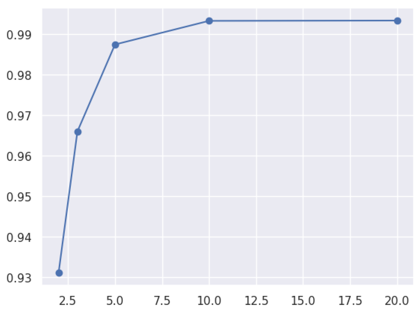
4.1.5. Random Forest

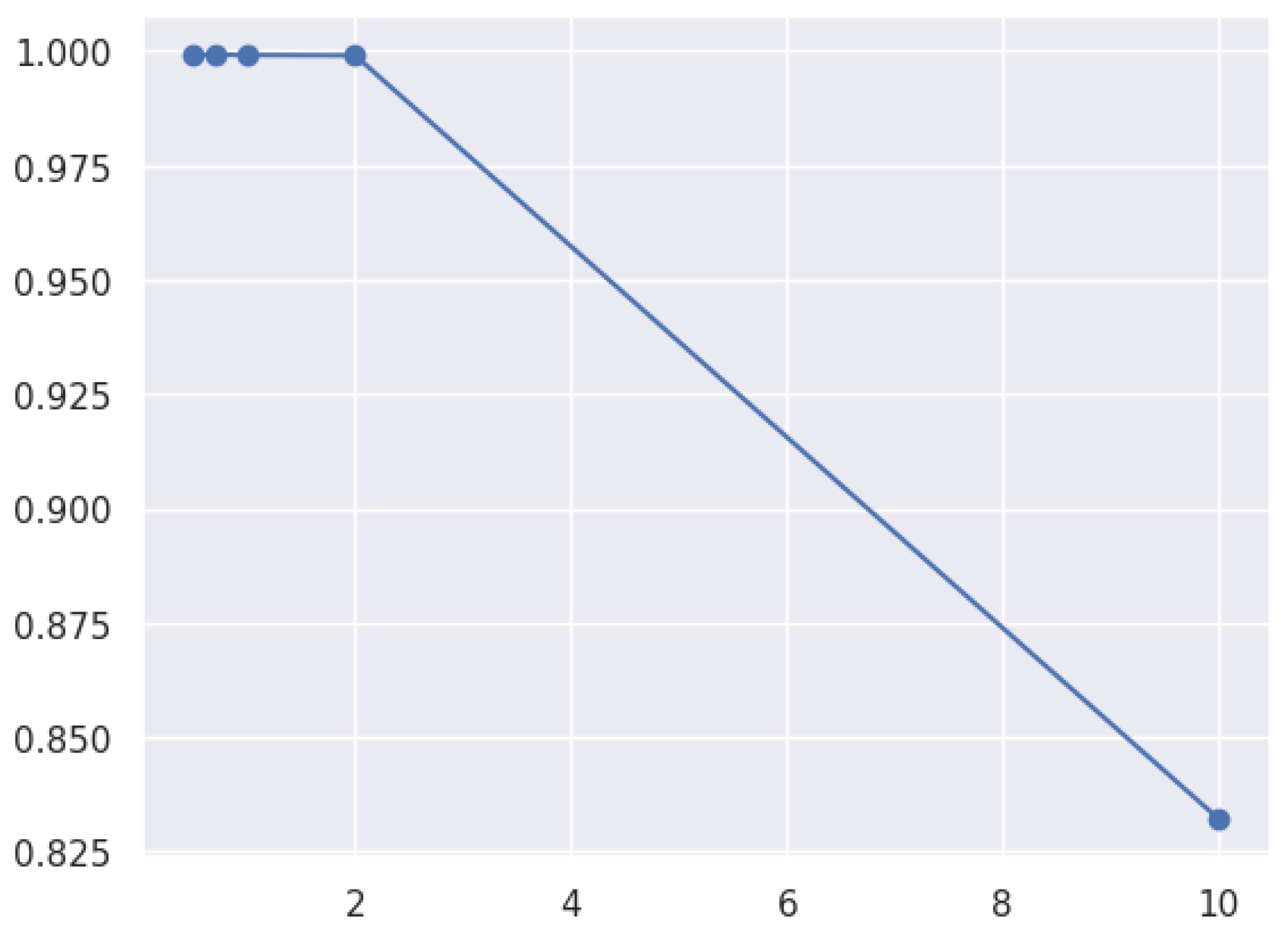
For the CIC-MalMem-2022 dataset, the accuracy result was 99.98%. As shown in Figure 33, the model correctly predicted 5808 malicious and 5803 benign instances. However, one malicious instance was incorrectly predicted as benign, and one benign instance was incorrectly predicted as malicious. For the CIC-IDS-2018 dataset, the accuracy result was 99.64%, with the confusion matrix shown in Figure 34. The model correctly predicted 2071 malicious and 4431 benign instances. Two malicious instances were incorrectly identified as benign, and twenty-four benign instances were incorrectly identified as malicious. For CIC-IDS-2017, the model achieved 99.40% accuracy; the confusion matrix in Figure 35 shows that the model correctly predicted 6287 malicious and 6985 benign instances. However, the model wrongly predicted 66 malicious samples as benign and 14 benign samples as malicious. The learning curve for CIC-MalMem-2022 in Figure 36 shows that the training score is close to 100%, which indicates that the Forest classifier can learn the training data effectively. The cross-validation score, however, is slightly lower than the training score. Figure 37 illustrates that the Random Forest model learns the CIC-IDS-2018 dataset effectively, since each cycle achieved 100% for learning; however, cross-validation shows a slightly lower percentage, starting at around 98.40% and declining to 96.1%. As shown in Figure 38, the CIC-IDS-2017 dataset’s learning curve indicates the training score begins at 99.71% accuracy and decreases to 99.52. However, the cross-validation score is slightly lower than the training score: it starts at 99.39% and increases to 99.45%. The best parameter for the CIC-MalMem-2022 dataset is 20. The mean test score attained is 99.90%, as seen in Figure 39. Furthermore, the mean duration required to obtain these scores is 0.059 s. The analysis of Figure 40 reveals that the CIC-IDS-2018 dataset attains its best performance when the parameter value is set to 10. The selection of this criterion correlates with an average examination score of 99.20% and an average time taken of 0.056 s. Moreover, drawing upon the evidence shown in Figure 41, one may deduce that the most favorable value for CIC-IDS-2017 is 20. The aforementioned conclusion is substantiated by the average test score of 99.34% and the average score time of 0.248 s.

4.1.6. XGBoost

For the CIC-MalMem-2022 dataset, this model achieved an accuracy rate of 99.96%. According to Figure 42, the model correctly predicted 5806 malicious and 5803 benign instances. However, one malicious instance was incorrectly predicted as benign, and three benign instances were incorrectly predicted as malicious. The accuracy result for the CIC-IDS-2018 dataset was 99.73%, and the confusion matrix in Figure 43 indicates that the model correctly predicted 2076 malicious and 4432 benign instances. However, only 1 malicious instance was incorrectly identified as benign, while 16 benign instances were incorrectly identified as malicious. In addition, on the CIC-IDS-2017 dataset, the model achieved 99.84% accuracy, with the confusion matrix shown in Figure 44 showing that the model correctly predicted 6288 malicious and 7044 benign instances. On the other hand, the model incorrectly predicted 7 malicious samples as benign and 13 benign samples as malicious. Figure 45 shows that the training score is 100% at every cycle, while the cross-validation score is between 99.83 and 99.89% accurate. As shown in Figure 46, the CIC-IDS-2018 learning curve shows a high training score and a high cross-validation score, and the training score does not plateau, indicating that the model does not overfit the data during the training phase. According to Figure 47, the training score for the CIC-IDS-2017 dataset oscillates between 100% and 99.99%, in contrast to the cross-validation score, which begins at 99.54% and then increases, reaching 99.90%. For the XGBoost model, the learning rate is a very important parameter. As shown in Figure 48, the best parameter for the CIC-MalMem-2022 dataset is 0.7, with a mean test score of 99.92%. According to Figure 49, the best parameter value for the CIC-IDS-2018 dataset is 0.5, with a mean test score of 99.50%. In addition, the best parameter value for the CIC-IDS-2017 dataset is 0.7, with a mean test score of 99.49%, as displayed in Figure 50.

4.2. Security Analysis Using an Adversarial Attack Model

We defined an adversarial model that includes new types of attacks and tested the model’s robustness in detecting them on a real dataset (CSE-CIC-IDS2018). First, we describe the adversarial attack model; then, we present the preprocessing and test methodology, and lastly, we show the obtained results and their analysis.

4.2.1. Adversarial Attack Model

Our adversarial attack model consists of four different types of attacks:

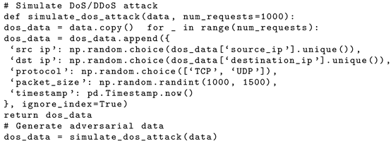
• DoS/DDoS: We simulated high-volume traffic from a single source and multiple sources to disrupt service availability. We used the same features, like packet rate, duration, and protocol type, to mimic attack patterns already existing in the real dataset (CSE-CIC-IDS2018).
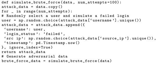
• Brute force: We simulated repeated login attempts with varying usernames and passwords to gain unauthorized access to the organization’s network or systems. Also, we used features like failed login attempts and source IP addresses.
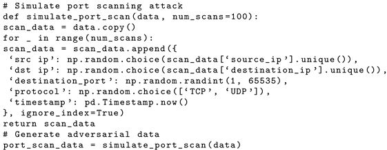
• Port scanning: We simulated a port scanning attack by sending packets to multiple ports to identify vulnerabilities in the organization’s network and systems. We used features like port numbers, packet count, and response time.
• Malware: We simulated a malicious payload delivery and execution attack to gain persistent access to or control of the organization’s systems. We used features like file size, execution behavior, and network activity.

4.2.2. Attack Generation and Preprocessing of Generated Attack Data

In this section, we will present some code snippets used to generate the attacks and preprocess the attack data to ensure consistency in modeling and a good fit with the dataset in terms of normalization, scaling, selected features, labeling, and handling missing data. Code Listing 1 simulates a DoS/DDoS attack by generating high-volume traffic to overwhelm the system:

Code Listing 2 simulates a brute force attack by generating repeated failed login attempts.

Code Listing 3 simulates a port scanning attack by generating scanning behavior data by sending packets to multiple ports.

Code Listing 4 simulates a malware attack by generating malicious payload delivery and execution data. Before testing the model, we preprocessed the generated attack data by performing the following:

• Ensure that the simulated adversarial data have the same features as the original dataset. Also, add new features related to new attacks when retraining the model to deal with data changes.
• Apply the same preprocessing steps to the simulated adversarial data as those applied to the original dataset.
• Ensure that the labels in the simulated adversarial data match the encoding used in the original dataset.
• Ensure that the simulated adversarial data follow the same statistical distribution as the original dataset. A significant change in data distribution requires retraining the model.

Listing 1. DoS/DDos simulated attack.

Listing 2. Brute force simulated attack.

Listing 3. Port scanning simulated attack.

Listing 4. Malware simulated attack.

4.2.3. Adversarial Model Results and Analysis

The XGBoost model was used to detect adversarial attacks because it is highly accurate and takes less time (faster model).

We used two different testing methods. The first involved testing the model based on the original dataset without retraining it by using the newly generated attack data to analyze the model’s robustness.

Table 9. Performance metrics for adversarial attack detection without retraining the model on adversarial data.

Adversarial Attack	Accuracy	Test Time
DoS/DDoS	99.61%	0.02 s
Brute force	99.57%	0.03 s
Port scanning	99.63%	0.02 s
Malware	99.63%	0.02 s

depicts the different metrics.

The XGBoost model was already evaluated on the CIC-IDS-2018 dataset and had an accuracy of 99.73% and a test time of 0.03 s. According to our evaluation, the XGBoost model’s detection accuracy on adversarial data without training on adversarial data ranges from 99.57% in detecting brute force attacks to 99.63% in detecting port scanning and malware attacks. We can observe that the accuracy is almost the same and the model keeps its ability to detect new attacks.

The second test method involved retraining the model by using the simulated attack data, which is required in the case of a significant change in data distribution. The results are depicted in

Table 10. Performance metrics for adversarial attack detection using trained model on adversarial data.

Adversarial Attacks	Accuracy	Test Time
Combined data	99.75%	0.03 s

.

Table 10 shows an accuracy in detection of 99.75%, which outperforms even the accuracy detection rate on the original data, which is 99.73%.

The confusion matrix in Figure 51 indicates that the model correctly predicted 1561 malicious and 4449 benign instances. Fourteen instances were incorrectly predicted as malicious, and one was incorrectly predicted as benign.

According to the results, it is clear that the model has the ability to detect new attacks while keeping high accuracy and a low false positive rate, which ensures the model’s robustness. Of course, in the case of an infrastructure change, such as adding new devices or changing the network topology, the model must be retrained based on the new data distribution to keep a high detection rate.

4.3. Discussion

According to

Table 11. CIC-MalMem-2022 dataset analysis.

Algorithm	Accuracy	Precision	Recall	F1-Score	Test Time
AdaBoost	99.94%	99.96%	99.93%	99.94%	0.10 s
Voting	99.96%	99.98%	99.94%	99.96%	2.27 s
Stacking	99.98%	99.98%	99.98%	99.98%	2.90 s
SVM	99.93%	99.89%	99.98%	99.93%	0.44 s
RF	99.98%	99.98%	99.98%	99.98%	0.11 s
XGBoost	99.96%	99.98%	99.94%	99.96%	0.01 s

,

Table 12. CIC-IDS-2018 dataset analysis.

Algorithm	Accuracy	Precision	Recall	F1-Score	Test Time
AdaBoost	99.11%	99.37%	97.86%	98.61%	0.08 s
Voting	99.58%	100%	98.71%	99.35%	2.20 s
Stacking	99.61%	99.66%	99.13%	99.40%	1.64 s
SVM	97.41%	97.96%	93.91%	95.89%	1.56 s
RF	99.64%	99.90%	98.99%	99.44%	0.10 s
XGBoost	99.73%	99.95%	99.23%	99.59%	0.03 s

and

Table 13. CIC-IDS-2017 dataset analysis.

Algorithm	Accuracy	Precision	Recall	F1-Score	Test Time
AdaBoost	98.64%	98.18%	98.95%	98.56%	0.11 s
Voting	99.31%	98.91%	99.65%	99.28%	4.66 s
Stacking	99.86%	99.66%	99.74%	99.85%	2.93 s
SVM	94.04%	89.39%	99.14%	94.01%	9.81 s
RF	99.40%	98.96%	98.96%	99.36%	0.18 s
XGBoost	99.84%	99.88%	99.79%	99.84%	0.04 s

, and the requirement of the proposed architecture, the fastest model to detect malicious instances is XGBoost, while Stacking gives the highest accuracy in detecting malicious instances. Also, the Stacking model has fewer FNs for all datasets. XGBoost exhibits high accuracy, recall, precision, and F1-score across all datasets, with very low test time. The Stacking approach achieves the highest accuracy and F1-score in some cases. Additionally, it achieves high recall and precision, but it has a longer test time.

Due to the importance of test time in this study, the experiment conducted by [34,37] was re-conducted to determine the test time. A comparison of this study’s results and other studies is shown in

Table 14. Comparative analysis of CIC-MalMem-2022 dataset.

Author	Feature Selection	Algorithm	Selected Features	Accuracy	Test Time
[34]	XGBoost	RF	20	100%	0.09 s
This study	SelectKBest	XGBoost	25	99.96%	0.01 s

,

Table 15. Comparative analysis of CIC-IDS-2018 Dataset.

Author	Feature Selection	Algorithm	Selected Features	Accuracy	Test Time
[24]	RF and PCA	LightGBM	37	97.73%	17.94 s
This study	VarianceThreshold	XGBoost	72	99.73%	0.03 s

and

Table 16. Comparative analysis of CIC-IDS-2017 Dataset.

Author	Feature Selection	Algorithm	Selected Features	Accuracy	Test Time
[37]	Correlation Heatmap	Voting classifier	10	96.25%	15.86 s
This study	SelectKBest	XGBoost	30	99.84%	0.04 s

for each dataset used in this study. This study achieved 99.96% accuracy on the CIC-MalMem-2022 dataset within 0.01 s, while [34] obtained 100% accuracy with a time of 0.08 s, which is higher than this study. Based on the CIC-IDS-2018 and CIC-IDS-2017 datasets, this study achieves greater accuracy and lower time than [24,37]. In other studies, there is no global centralized traffic inspection before traffic is distributed to the sub-networks of an organization, as instead occurs with a multi-model IDS based on the traffic load. The proposed architecture involves two layers of security. The multi-model IDS in the first layer inspects the organization’s incoming traffic quickly. In contrast, the IDSs in the sub-networks of the organization act as second-layer security, which can more accurately detect attacks.

This research study aims to analyze traffic behavior and patterns; each network traffic has IP addresses, protocols, and packet sizes. While this study was evaluated by using specific datasets, the proposed architecture of a multi-model IDS based on traffic load was designed to be adaptable to different scenarios. Additionally, the proposed architecture allows organizations to monitor incoming traffic and encrypt sensitive data while restricting access to authorized users only.

The percentage of accuracy of the ML-based IDS for different organizations depends on the nature of an organization’s data. If the data for a specific organization are private and sensitive, the risk becomes high. In this situation, the organization should focus on high accuracy despite the higher computational cost. On the other hand, if the data are not sensitive and are normal, the risk is lower. It is important to note that false positives and false negatives have different consequences based on the environment, circumstances, and current situation. False positives lead to unnecessary costs, and the model cannot distinguish between normal and malicious traffic. False negatives lead to high risk, so high accuracy is very important. By understanding the trade-offs between accuracy and computational cost, organizations can improve their systems to reduce risk.

Our multi-model IDS based on traffic load employs a combination of signature and behavior-based detection to address known and unknown threats. Signature-based detection is effective in detecting known patterns of attacks. On the other hand, the behavior-based detection approach analyzes the deviation from normal traffic. It is, therefore, capable of detecting zero-day exploits and Advanced Persistent Threats (APTs) that are not matched by existing signatures.

In the case of a change in the organization’s network topology and device types or a huge change in traffic, the model must be retrained on the new data after the change. Generally, organizations do not frequently change their network infrastructure, so the update rate of the model will not be frequent.

Limitations of Proposed Model

The multi-model based IDS was tested on a dataset using real traffic (CIC-IDS-2018) and on another using simulated traffic (CIC-IDS-2017). Although the results are promising, we would need to collect a much larger dataset of real-world traffic and use techniques such as data augmentation to avoid overfitting. However, it should be noted that the proposed architecture remains to be deployed in a real-world setting.

5. Conclusions

The literature review examined various contemporary IDSs that utilize ML techniques across various environments. These techniques include information-based, similarity-based, probability-based, and error-based learning. The review also explored hybrid and SDN models in this context. This paper has undertaken a comprehensive literature research to improve NIDSs using ML techniques. Using a new architecture design, the proposed IDS is designed to scan all servers’ incoming traffic and redirect it to the requested server by creating a centralized proxy server. A two-layer security-based mechanism is proposed. Before reaching the central server, a preliminary layer of security is implemented, including examining global traffic. The second layer of security is implemented when the network traffic is dispersed from the central server to the sub-networks of the organization.

This paper presents and analyzes the results of the AdaBoost, Voting, Stacking, Support Vector Machine, Random Forest, and XGBoost models on the CIC-MalMem-2022, CIC-IDS-2018, and CIC-IDS-2017 datasets. The results show that XGBoost and Stacking are the best models. The first model used is XGBoost, which can perform the rapid identification of harmful instances. Subsequently, a Stacking classifier is utilized as the second model, demonstrating a notable level of accuracy but necessitating an extended detection duration. The activation of each model will be determined based on the volume of network traffic. The determination of the threshold value, which accurately represents the level of network traffic, is undertaken by the network administrator. The activation of the quickest model occurs when the amount of traffic is above the predetermined threshold value. Alternatively, the model with greater accuracy and longer detection times will be engaged. For the second layer, the Stacking model is used. They achieve a high level of accuracy in detecting harmful activities.

The findings of this experiment indicate that the XGBoost model exhibits the highest speed in identifying malicious data across all three datasets (CIC-MalMem-2022, CIC-IDS-2018, and CIC-IDS-2017). Conversely, the Stacking approach demonstrates the highest accuracy in this context. However, identifying fraudulent material necessitates a more significant amount of time. Based on the findings of the XGBoost model, on the CIC-MalMem-2022, CIC-IDS-2018, and CIC-IDS-2017 datasets, it exhibits accuracy rates of 99.96%, 99.73%, and 99.84%, respectively, achieved within time intervals of 0.01 s, 0.03 s, and 0.04 s, respectively. The Stacking model achieved accuracy values of 99.98%, 99.61%, and 99.86% on the CIC-MalMem-2022, CIC-IDS-2018, and CIC-IDS-2017 datasets, respectively. The findings indicate that the multi-model IDS that relies on traffic load is significantly capable of efficiently identifying and detecting malicious activity. The proposed model emphasizes the implementation of global traffic inspections before ingress into an organization’s network, as well as the implementation of two-layer security strategies. The proposed model also inspects the entire traffic with a faster model and inspects the subdomains with high accuracy at all times. Compared with other IDS models, the proposed XGBoost model has high accuracy and efficiency.

Although the proposed multi-model IDS is comparable to existing solutions in terms of accuracy, analyzing performance metrics reveals additional insights. The precision, F1-score, and recall of the system were carefully considered, showing its ability to identify true positives while minimizing false positives at the same time. In addition to its robust generalization across diverse datasets and simulated network traffic scenarios, the proposed multi-model IDS can adapt to varying threat landscapes, demonstrating its efficiency in dynamic environments.

The proposed model can be improved in several ways. For instance, the IPS prevention of malicious IPs through firewalls can be accomplished automatically by using a threat intelligence feed. The UNSW-NB15 dataset will be used. We also plan to focus on the network architecture inside an authentic setting pertaining to a particular business. Subsequently, we will proceed to perform an empirical investigation within this real-world environment, wherein we will gather relevant traffic data. These data will be appropriately processed and formatted to align with the models used in this paper. Deep learning algorithms may represent a good alternative to conduct this kind of learning and analysis.

References

1. Fakieh, A.; Akremi, A. An Effective Blockchain-Based Defense Model for Organizations against Vishing Attacks. Appl. Sci. 2022, 12, 13020. [Google Scholar] [CrossRef]
2. Azizan, A.H.; Mostafa, S.A.; Mustapha, A.; Foozy, C.F.M.; Wahab, M.H.A.; Mohammed, M.A.; Khalaf, B.A. A machine learning approach for improving the performance of network intrusion detection systems. Ann. Emerg. Technol. Comput. (AETiC) 2021, 5, 201–208. [Google Scholar] [CrossRef]
3. Priyadarsini, M.; Bera, P. Software defined networking architecture, traffic management, security, and placement: A survey. Comput. Netw. 2021, 192, 108047. [Google Scholar] [CrossRef]
4. Samantaray, M.; Satapathy, S.; Lenka, A. A Systematic Study on Network Attacks and Intrusion Detection System. In Machine Intelligence and Data Science Applications: Proceedings of MIDAS 2021; Springer: Berlin/Heidelberg, Germany, 2022; pp. 195–210. [Google Scholar]
5. Akremi, A.; Sallay, H.; Rouached, M. Intrusion detection systems alerts reduction: New approach for forensics readiness. In Security and Privacy Management, Techniques, and Protocols; IGI Global: Hershey, PA, USA, 2018; pp. 255–275. [Google Scholar]
6. Soomro, A.M.; Naeem, A.B.; Ghafoor, M.I.; Senapati, B.; Rajwana, M.A. A Systematic Review of Artificial Intelligence Techniques Used for IDS Analysis. J. Comput. Biomed. Inform. 2023, 5, 52–67. [Google Scholar]
7. Jaradat, A.S.; Barhoush, M.M.; Easa, R.B. Network intrusion detection system: Machine learning approach. Indones. J. Electr. Eng. Comput. Sci. 2022, 25, 1151–1158. [Google Scholar] [CrossRef]
8. Amanoul, S.V.; Abdulazeez, A.M.; Zeebare, D.Q.; Ahmed, F.Y. Intrusion detection systems based on machine learning algorithms. In Proceedings of the 2021 IEEE International Conference on Automatic Control & Intelligent Systems (I2CACIS), Shah Alam, Malaysia, 26 June 2021; pp. 282–287. [Google Scholar]
9. Verma, A.; Ranga, V. Machine learning based intrusion detection systems for IoT applications. Wirel. Pers. Commun. 2020, 111, 2287–2310. [Google Scholar] [CrossRef]
10. Mirlekar, S.; Kanojia, K.P. A Study on Taxonomy and State-of-the-Art Intrusion Detection System. In Proceedings of the 2nd International Conference on Advancement in Electronics & Communication Engineering (AECE 2022), Ghaziabad, India, 14–15 July 2022. [Google Scholar]
11. Unnisa A, N.; Yerva, M.; Kurian, M.Z. Review on Intrusion Detection System (IDS) for Network Security using Machine Learning Algorithms. Int. Res. J. Adv. Sci. Hub 2022, 4, 67–74. [Google Scholar] [CrossRef]
12. Aljanabi, M.; Ismail, M.A.; Ali, A.H. Intrusion detection systems, issues, challenges, and needs. Int. J. Comput. Intell. Syst. 2021, 14, 560–571. [Google Scholar] [CrossRef]
13. Alajanbi, M.; Ismail, M.A.; Hasan, R.A.; Sulaiman, J. Intrusion Detection: A Review. Mesopotamian J. Cybersecur. 2021, 2021, 1–4. [Google Scholar] [CrossRef]
14. Akremi, A.; Sallay, H.; Rouached, M. An efficient intrusion alerts miner for forensics readiness in high speed networks. Int. J. Inf. Secur. Priv. (IJISP) 2014, 8, 62–78. [Google Scholar] [CrossRef]
15. Yan, F.; Wen, S.; Nepal, S.; Paris, C.; Xiang, Y. Explainable machine learning in cybersecurity: A survey. Int. J. Intell. Syst. 2022, 37, 12305–12334. [Google Scholar]
16. Jahwar, A.F.; Ameen, S.Y. A review on cybersecurity based on machine learning and deep learning algorithms. J. Soft Comput. Data Min. 2021, 2, 14–25. [Google Scholar]
17. Robles Herrera, S.; Ceberio, M.; Kreinovich, V. When is deep learning better and when is shallow learning better: Qualitative analysis. Int. J. Parallel Emergent Distrib. Syst. 2022, 37, 589–595. [Google Scholar] [CrossRef]
18. Sarker, I.H. Machine learning: Algorithms, real-world applications and research directions. SN Comput. Sci. 2021, 2, 160. [Google Scholar] [CrossRef]
19. Demertzis, K.; Kostinakis, K.; Morfidis, K.; Iliadis, L. A comparative evaluation of machine learning algorithms for the prediction of R/C buildings’ seismic damage. arXiv 2022, arXiv:2203.13449. [Google Scholar]
20. Kelleher, J.D.; Mac Namee, B.; D’arcy, A. Fundamentals of Machine Learning for Predictive Data Analytics: Algorithms, Worked Examples, and Case Studies; MIT Press: Cambridge, MA, USA, 2020. [Google Scholar]
21. Das, S.; Gangwani, P.; Upadhyay, H. Integration of machine learning with cybersecurity: Applications and challenges. In Artificial Intelligence in Cyber Security: Theories and Applications; Springer: Berlin/Heidelberg, Germany, 2023; pp. 67–81. [Google Scholar]
22. Attou, H.; Guezzaz, A.; Benkirane, S.; Azrour, M.; Farhaoui, Y. Cloud-Based Intrusion Detection Approach Using Machine Learning Techniques. Big Data Min. Anal. 2023, 6, 311–320. [Google Scholar]
23. Saheed, Y.K.; Abiodun, A.I.; Misra, S.; Holone, M.K.; Colomo-Palacios, R. A machine learning-based intrusion detection for detecting internet of things network attacks. Alex. Eng. J. 2022, 61, 9395–9409. [Google Scholar] [CrossRef]
24. Seth, S.; Singh, G.; Kaur Chahal, K. A novel time efficient learning-based approach for smart intrusion detection system. J. Big Data 2021, 8, 111. [Google Scholar]
25. Ding, H.; Chen, L.; Dong, L.; Fu, Z.; Cui, X. Imbalanced data classification: A KNN and generative adversarial networks-based hybrid approach for intrusion detection. Future Gener. Comput. Syst. 2022, 131, 240–254. [Google Scholar]
26. Dini, P.; Saponara, S. Analysis, design, and comparison of machine-learning techniques for networking intrusion detection. Designs 2021, 5, 9. [Google Scholar] [CrossRef]
27. Hnamte, V.; Balram, G.; Priyanka, V.; Kolluru, V. Implementation of Naive Bayes Classifier for Reducing DDoS Attacks in IoT Networks. J. Algebr. Stat. 2022, 13, 2749–2757. [Google Scholar]
28. Onah, J.O.; Abdullahi, S.M.; Abdullahi, M.; Hassan, I.H.; Al-Ghusham, A. Genetic Algorithm based feature selection and Naïve Bayes for anomaly detection in fog computing environment. Mach. Learn. Appl. 2021, 6, 100156. [Google Scholar]
29. Baniasadi, S.; Rostami, O.; Martín, D.; Kaveh, M. A novel deep supervised learning-based approach for intrusion detection in IoT systems. Sensors 2022, 22, 4459. [Google Scholar] [CrossRef] [PubMed]
30. Naveed, M.; Arif, F.; Usman, S.M.; Anwar, A.; Hadjouni, M.; Elmannai, H.; Hussain, S.; Ullah, S.S.; Umar, F. A Deep Learning-Based Framework for Feature Extraction and Classification of Intrusion Detection in Networks. Wirel. Commun. Mob. Comput. 2022, 2022, 2215852. [Google Scholar]
31. Ponmalar, A.; Dhanakoti, V. An intrusion detection approach using ensemble support vector machine based chaos game optimization algorithm in big data platform. Appl. Soft Comput. 2022, 116, 108295. [Google Scholar]
32. Ullah, I.; Mahmoud, Q.H. Design and development of a deep learning-based model for anomaly detection in IoT networks. IEEE Access 2021, 9, 103906–103926. [Google Scholar]
33. Hnamte, V.; Hussain, J. DCNNBiLSTM: An Efficient Hybrid Deep Learning-Based Intrusion Detection System. Telemat. Inform. Rep. 2023, 10, 100053. [Google Scholar]
34. Talukder, M.A.; Hasan, K.F.; Islam, M.M.; Uddin, M.A.; Akhter, A.; Yousuf, M.A.; Alharbi, F.; Moni, M.A. A dependable hybrid machine learning model for network intrusion detection. J. Inf. Secur. Appl. 2023, 72, 103405. [Google Scholar]
35. Balyan, A.K.; Ahuja, S.; Lilhore, U.K.; Sharma, S.K.; Manoharan, P.; Algarni, A.D.; Elmannai, H.; Raahemifar, K. A hybrid intrusion detection model using ega-pso and improved random forest method. Sensors 2022, 22, 5986. [Google Scholar] [CrossRef]
36. Akshay Kumaar, M.; Samiayya, D.; Vincent, P.; Srinivasan, K.; Chang, C.Y.; Ganesh, H. A Hybrid Framework for Intrusion Detection in Healthcare Systems Using Deep Learning. Front. Public Health 2022, 9, 824898. [Google Scholar]
37. Patil, S.; Varadarajan, V.; Mazhar, S.M.; Sahibzada, A.; Ahmed, N.; Sinha, O.; Kumar, S.; Shaw, K.; Kotecha, K. Explainable artificial intelligence for intrusion detection system. Electronics 2022, 11, 3079. [Google Scholar] [CrossRef]
38. Rincy N, T.; Gupta, R. Design and development of an efficient network intrusion detection system using machine learning techniques. Wirel. Commun. Mob. Comput. 2021, 2021, 9974270. [Google Scholar]
39. Dutta, V.; Choraś, M.; Kozik, R.; Pawlicki, M. Hybrid model for improving the classification effectiveness of network intrusion detection. In Proceedings of the 13th International Conference on Computational Intelligence in Security for Information Systems (CISIS 2020), Burgos, Spain, 24–26 June 2020; Springer: Berlin/Heidelberg, Germany, 2021; pp. 405–414. [Google Scholar]
40. Liu, C.; Gu, Z.; Wang, J. A hybrid intrusion detection system based on scalable K-Means+ random forest and deep learning. IEEE Access 2021, 9, 75729–75740. [Google Scholar]
41. Aldallal, A.; Alisa, F. Effective intrusion detection system to secure data in cloud using machine learning. Symmetry 2021, 13, 2306. [Google Scholar] [CrossRef]
42. Elsayed, R.A.; Hamada, R.A.; Abdalla, M.I.; Elsaid, S.A. Securing IoT and SDN systems using deep-learning based automatic intrusion detection. Ain Shams Eng. J. 2023, 14, 102211. [Google Scholar]
43. Chaganti, R.; Suliman, W.; Ravi, V.; Dua, A. Deep Learning Approach for SDN-Enabled Intrusion Detection System in IoT Networks. Information 2023, 14, 41. [Google Scholar] [CrossRef]
44. Alzahrani, A.O.; Alenazi, M.J. Designing a network intrusion detection system based on machine learning for software defined networks. Future Internet 2021, 13, 111. [Google Scholar] [CrossRef]
45. Javeed, D.; Gao, T.; Khan, M.T.; Ahmad, I. A hybrid deep learning-driven SDN enabled mechanism for secure communication in Internet of Things (IoT). Sensors 2021, 21, 4884. [Google Scholar] [CrossRef]
46. Perez-Diaz, J.A.; Valdovinos, I.A.; Choo, K.K.R.; Zhu, D. A flexible SDN-based architecture for identifying and mitigating low-rate DDoS attacks using machine learning. IEEE Access 2020, 8, 155859–155872. [Google Scholar]
47. Alharbi, A.; Alsubhi, K. Botnet detection approach using graph-based machine learning. IEEE Access 2021, 9, 99166–99180. [Google Scholar]
48. Wang, X.; Zhu, T.; Xia, M.; Liu, Y.; Wang, Y.; Wang, X.; Zhuang, L.; Zhong, D.; Weng, S.; Zhu, J.; et al. Predicting the Prognosis of Patients in the Coronary Care Unit via Machine Learning Using XGBoost. Front. Front. Cardiovasc. Med. 2021, 9, 1–13. [Google Scholar]
49. Urrea, C.; Benítez, D. Software-defined networking solutions, architecture and controllers for the industrial internet of things: A review. Sensors 2021, 21, 6585. [Google Scholar] [CrossRef] [PubMed]
50. Shetabi, M.; Akbari, A. SAHAR: A control plane architecture for high available software-defined networks. Int. J. Commun. Netw. Distrib. Syst. 2020, 24, 409–440. [Google Scholar]
51. Valdovinos, I.A.; Pérez-Díaz, J.A.; Choo, K.K.R.; Botero, J.F. Emerging DDoS attack detection and mitigation strategies in software-defined networks: Taxonomy, challenges and future directions. J. Netw. Comput. Appl. 2021, 187, 103093. [Google Scholar]
52. Ahmad, S.; Mir, A.H. Scalability, consistency, reliability and security in SDN controllers: A survey of diverse SDN controllers. J. Netw. Syst. Manag. 2021, 29, 9. [Google Scholar]
53. Khan, K.; Mehmood, A.; Khan, S.; Khan, M.A.; Iqbal, Z.; Mashwani, W.K. A survey on intrusion detection and prevention in wireless ad-hoc networks. J. Syst. Archit. 2020, 105, 101701. [Google Scholar]
54. Chen, S.; Wu, Z.; Christofides, P.D. Cyber-security of centralized, decentralized, and distributed control-detector architectures for nonlinear processes. Chem. Eng. Res. Des. 2021, 165, 25–39. [Google Scholar]
55. Helmy, A.; Nayak, A. Centralized vs. decentralized bandwidth allocation for supporting green fog integration in next-generation optical access networks. IEEE Commun. Mag. 2020, 58, 33–39. [Google Scholar]
56. Louk, M.H.L.; Tama, B.A. Tree-Based Classifier Ensembles for PE Malware Analysis: A Performance Revisit. Algorithms 2022, 15, 332. [Google Scholar] [CrossRef]
57. Qazi, E.U.H.; Faheem, M.H.; Zia, T. HDLNIDS: Hybrid Deep-Learning-Based Network Intrusion Detection System. Appl. Sci. 2023, 13, 4921. [Google Scholar] [CrossRef]
58. Hassan, I.H.; Abdullahi, M.; Aliyu, M.M.; Yusuf, S.A.; Abdulrahim, A. An improved binary manta ray foraging optimization algorithm based feature selection and random forest classifier for network intrusion detection. Intell. Syst. Appl. 2022, 16, 200114. [Google Scholar]
59. Killamsetty, K.; Sivasubramanian, D.; Ramakrishnan, G.; Iyer, R. Glister: Generalization based data subset selection for efficient and robust learning. In Proceedings of the AAAI Conference on Artificial Intelligence, Vancouver, BC, Canada, 2–9 February 2021; Volume 35, pp. 8110–8118. [Google Scholar]
60. Pudjihartono, N.; Fadason, T.; Kempa-Liehr, A.W.; O’Sullivan, J.M. A review of feature selection methods for machine learning-based disease risk prediction. Front. Bioinform. 2022, 2, 927312. [Google Scholar]
61. Izquierdo, C.; Casas, G.; Martin-Isla, C.; Campello, V.M.; Guala, A.; Gkontra, P.; Rodríguez-Palomares, J.F.; Lekadir, K. Radiomics-based classification of left ventricular non-compaction, hypertrophic cardiomyopathy, and dilated cardiomyopathy in cardiovascular magnetic resonance. Front. Cardiovasc. Med. 2021, 8, 764312. [Google Scholar]
62. Brownlee, J. Data Preparation for Machine Learning: Data Cleaning, Feature Selection, and Data Transforms in Python; Machine Learning Mastery: Melbourne, Australia, 2020. [Google Scholar]
63. Zhang, Y.; Wang, H.; Chen, W.; Zeng, J.; Zhang, L.; Wang, H.; Weinan, E. DP-GEN: A concurrent learning platform for the generation of reliable deep learning based potential energy models. Comput. Phys. Commun. 2020, 253, 107206. [Google Scholar]
64. Linardatos, P.; Papastefanopoulos, V.; Kotsiantis, S. Explainable ai: A review of machine learning interpretability methods. Entropy 2020, 23, 18. [Google Scholar] [CrossRef] [PubMed]
65. Verma, R.; Nagar, V.; Mahapatra, S. Introduction to supervised learning. In Data Analytics in Bioinformatics: A Machine Learning Perspective; John Wiley & Sons: Hoboken, NJ, USA, 2021; pp. 1–34. [Google Scholar]
66. Ren, J.; Zhang, M.; Yu, C.; Liu, Z. Balanced mse for imbalanced visual regression. In Proceedings of the IEEE/CVF Conference on Computer Vision and Pattern Recognition, New Orleans, LA, USA, 18–24 June 2022; pp. 7926–7935. [Google Scholar]
67. Vázquez, F.I.; Hartl, A.; Zseby, T.; Zimek, A. Anomaly detection in streaming data: A comparison and evaluation study. Expert Syst. Appl. 2023, 233, 120994. [Google Scholar]
68. Mohr, F.; van Rijn, J.N. Learning Curves for Decision Making in Supervised Machine Learning—A Survey. arXiv 2022, arXiv:2201.12150. [Google Scholar]
69. Géron, A. Hands-On Machine Learning with Scikit-Learn, Keras, and TensorFlow; O’Reilly Media, Inc.: Sebastopol, CA, USA, 2022. [Google Scholar]
70. Hamida, S.; El Gannour, O.; Cherradi, B.; Ouajji, H.; Raihani, A. Optimization of machine learning algorithms hyper-parameters for improving the prediction of patients infected with COVID-19. In Proceedings of the 2020 IEEE 2nd International Conference on Electronics, Control, Optimization and Computer Science (ICECOCS), Kenitra, Morocco, 2–3 December 2020; pp. 1–6. [Google Scholar]
71. Yu, T.; Zhu, H. Hyper-parameter optimization: A review of algorithms and applications. arXiv 2020, arXiv:2003.05689. [Google Scholar]
Figure 1. Multi-model based on network traffic load.
Network 05 00013 g001
Figure 2. Machine learning model architecture.
Network 05 00013 g002
Figure 3. Confusion matrix for AdaBoost on CIC-MalMem-2022 dataset.
Network 05 00013 g003
Figure 4. Confusion matrix for AdaBoost on CIC-IDS-2018 dataset.
Network 05 00013 g004
Figure 5. Confusion matrix for AdaBoost on CIC-IDS-2017 dataset.
Network 05 00013 g005
Figure 6. Learning curve for AdaBoost on CIC-MalMem-2022 dataset.
Network 05 00013 g006
Figure 7. Learning curve for AdaBoost on CIC-IDS-2018 dataset.
Network 05 00013 g007
Figure 8. Learning curve for AdaBoost on CIC-IDS-2017 dataset.
Network 05 00013 g008
Figure 9. Hyperparameter tuning for AdaBoost on CIC-MalMem-2022 dataset.
Network 05 00013 g009
Figure 10. Hyperparameter tuning for AdaBoost on CIC-IDS-2018 dataset.
Network 05 00013 g010
Figure 11. Hyperparameter tuning for AdaBoost on CIC-IDS-2017 dataset.
Network 05 00013 g011
Figure 12. Confusion matrix for Voting classifier on CIC-MalMem-2022 dataset.
Network 05 00013 g012
Figure 13. Confusion matrix for Voting classifier on CIC-IDS-2018 dataset.
Network 05 00013 g013
Figure 14. Confusion matrix for Voting classifier on CIC-IDS-2017 dataset.
Network 05 00013 g014
Figure 15. Learning curve for Voting classifier on CIC-MalMem-2022 dataset.
Network 05 00013 g015
Figure 16. Learning curve for Voting classifier on CIC-IDS-2018 dataset.
Network 05 00013 g016
Figure 17. Learning curve for Voting classifier on CIC-IDS-2017 dataset.
Network 05 00013 g017
Figure 18. Confusion matrix for Stacking classifier on CIC-MalMem-2022 dataset.
Network 05 00013 g018
Figure 19. Confusion matrix for Stacking classifier on CIC-IDS-2018 dataset.
Network 05 00013 g019
Figure 20. Confusion matrix for Stacking classifier on CIC-IDS-2017 dataset.
Network 05 00013 g020
Figure 21. Learning curve for Stacking classifier on CIC-MalMem-2022 dataset.
Network 05 00013 g021
Figure 22. Learning curve for Stacking classifier on CIC-IDS-2018 dataset.
Network 05 00013 g022
Figure 23. Learning curve for Stacking classifier on CIC-IDS-2017 dataset.
Network 05 00013 g023
Figure 24. Confusion matrix for SVM on CIC-MalMem-2022 dataset.
Network 05 00013 g024
Figure 25. Confusion matrix for SVM on CIC-IDS-2018 dataset.
Network 05 00013 g025
Figure 26. Confusion matrix for SVM on CIC-IDS-2017 dataset.
Network 05 00013 g026
Figure 27. Learning curve for SVM on CIC-MalMem-2022 dataset.
Network 05 00013 g027
Figure 28. Learning curve for SVM on CIC-IDS-2018 dataset.
Network 05 00013 g028
Figure 29. Learning curve for SVM on CIC-IDS-2017 dataset.
Network 05 00013 g029
Figure 30. Hyperparameter tuning for SVM on CIC-MalMem-2022 dataset.
Network 05 00013 g030
Figure 31. Hyperparameter tuning for SVM on CIC-IDS-2018 dataset.
Network 05 00013 g031
Figure 32. Hyperparameter tuning for SVM on CIC-IDS-2017 dataset.
Network 05 00013 g032
Figure 33. Confusion matrix for RF on CIC-MalMem-2022.
Network 05 00013 g033
Figure 34. Confusion matrix for RF on CIC-IDS-2018.
Network 05 00013 g034
Figure 35. Confusion matrix for RF on CIC-IDS-2017.
Network 05 00013 g035
Figure 36. Learning curve for RF on CIC-MalMem-2022.
Network 05 00013 g036
Figure 37. Learning curve for RF on CIC-IDS-2018.
Network 05 00013 g037
Figure 38. Learning curve for RF on CIC-IDS-2017.
Network 05 00013 g038
Figure 39. Hyperparameter tuning for RF on CIC-MalMem-2022.
Network 05 00013 g039
Figure 40. Hyperparameter tuning for RF on CIC-IDS-2018.
Network 05 00013 g040
Figure 41. Hyperparameter tuning for RF on CIC-IDS-2017.
Network 05 00013 g041
Figure 42. Confusion matrix for XGBoost on CIC-MalMem-2022 dataset.
Network 05 00013 g042
Figure 43. Confusion matrix for XGBoost on CIC-IDS-2018 dataset.
Network 05 00013 g043
Figure 44. Confusion matrix for XGBoost on CIC-IDS-2017 dataset.
Network 05 00013 g044
Figure 45. Learning curve for XGBoost on CIC-MalMem-2022 dataset.
Network 05 00013 g045
Figure 46. Learning curve for XGBoost on CIC-IDS-2018 dataset.
Network 05 00013 g046
Figure 47. Learning curve for XGBoost on CIC-IDS-2017 dataset.
Network 05 00013 g047
Figure 48. Hyperparameter tuning for XGBoost on CIC-MalMem-2022 dataset.
Network 05 00013 g048
Figure 49. Hyperparameter tuning for XGBoost on CIC-IDS-2018 dataset.
Network 05 00013 g049
Figure 50. Hyperparameter tuning for XGBoost on CIC-IDS-2017 dataset.
Network 05 00013 g050
Figure 51. Confusion matrix trained on both the CIC-IDS-2018 dataset and the simulated attack data for XGBoost.
Network 05 00013 g051