An Experimental Comparison of Basic Device Localization Systems in Wireless Sensor Networks

Abstract

Localization plays a crucial role in wireless sensor networks (WSNs) and it has sparked significant research interest. GPSs provide quite accurate positioning estimations, but they are ineffective indoors and in environments like underwater. Power usage and cost are further disadvantages, and so many alternatives have been proposed. Many works in the literature still base localization on RSSI measurements and often rely on methods to mitigate the effects of fluctuations in values, so it is important to know real values of RSSIs measured using common devices. This work presents the main localization techniques and exploits a real testbed to collect and evaluate RSSI measurements. An accuracy evaluation and a comparison among several localization techniques are also provided.

1. Introduction

Recently, the ability to localize persons and objects has become the driving force behind a new context of applications, ranging from environment monitoring to navigation, warehouse management, safety, and entertainment. Developments in telecommunications and electronics have enabled the spread of micro-sensors able to send data via radio through a wireless sensor network (WSN). A WSN consists of numerous small, low-energy, low-cost sensors with limited processing power that communicate in an ad hoc manner. Localization, or positioning, is the process of determining the physical coordinates of these sensor nodes and is essential for applications that require knowledge of the event’s origin. Different localization methods have been proposed according to application requirements, most of them exploiting radio signals that can provide indirect information to estimate the sender position.

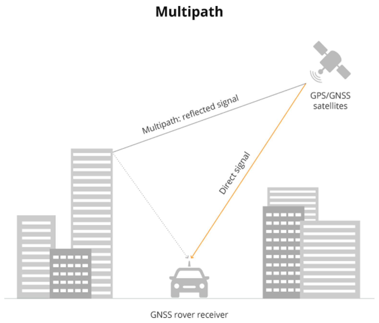
Localization in outdoor environments often relies on the Global Positioning System (GPS). This technology is not the best option for sensor nodes that usually run on limited power provided by batteries. Also, the cost of GPS modules is quite high, and they significantly increase the weight and the dimensions of the sensors. Shadowing and multipath have an impact on this technology’s accuracy. The shadowing effect is caused by the obstruction of the signal due to physical obstacles, moving or stationary, that the signal encounters in its path. Electromagnetic waves tend to be disturbed by objects that are the same size as the wavelength. Potentially any obstacle can be a source of disturbance in the 2.4 GHz band used by GPS. The multipath phenomenon [1], as shown in Figure 1, introduces both constructive and destructive interferences [2] since different signals may travel different paths to reach their destination. Nevertheless, the indoor reception from satellites is degraded due to signal attenuation caused by obstacles. Hence, localization in WSN adopts different solutions, especially indoors.

As transmissions in a WSN happen via radio, these signals provide an indirect way to calculate the sensor position and then localize objects or persons. This work presents some of the techniques available, and it mainly focuses on the use of a received signal strength indicator (RSSI). This parameter can be used to estimate the distance between a transmitter and a receiver and does not require any additional modules or circuitry as it is inherently supported by most chips. Unlike more complex localization techniques, such as those relying on time-of-flight or angle-of-arrival measurements, RSSI-based localization can be implemented with low-cost, off-the-shelf hardware, such as simple wireless transceivers or low-power microcontrollers. These components are widely available and inexpensive, reducing the overall cost of the sensor network. Furthermore, because RSSI is a relative measure, it does not require sophisticated hardware or additional infrastructure, such as GPSs or specialized sensors. This makes it an ideal choice for developing non-complex sensor systems that are suitable for large-scale deployments in resource-constrained environments. By leveraging RSSI for localization, wireless sensor networks can be built with minimal hardware and maintenance requirements.

The primary contribution of this work lies in the development and evaluation of a real testbed for RSSI-based localization within a WSN, which provides valuable insights into the practical application of basic localization techniques in real-world conditions. While this study does not introduce novel filtering algorithms or complex methodologies, it lays a crucial foundation by implementing a functional sensor network, conducting a series of controlled experiments, and comparing basic RSSI-based localization techniques in various scenarios. By constructing and testing a real-world testbed, this work offers practical benchmarks and empirical data, which are essential for understanding the limitations and performance of existing approaches. The results from these experiments provide a basis for future research, offering a clear path forward for developing more advanced localization systems, incorporating filtering techniques or machine learning methods.

The following section presents several localization approaches and how RSSI is still considered a base for the evaluation of sensor positions. In Section 3 and Section 4, the main localization techniques and the main localization algorithms are presented. In Section 5 the testbed and its implementation are described. In the same section, a link to the code developed and used for the testbed is available. A comparison of the outcomes of several localization methods and an assessment of their correctness are presented in Section 6, and Section 7 reports the conclusions.

2. Related Work

Although widely investigated, RSSI is still attracting interest as a localization method. The authors in [3] examine a variety of technologies and approaches for both indoor and outdoor localization. Accuracy, cost, complexity, security, scalability, and other issues are covered, along with many applications where location data are essential. Different wireless-based locating systems’ accuracy values are compared in urban, rural, indoor, and remote settings. The transmission scale affects the accuracy requirements, which in turn affects the kinds of applications that each localization approach can serve. This emphasizes how crucial localization is to wireless systems, both present and future, in all scenarios and applications. The work in [4] reviews various range-based and range-free localization techniques, with a focus on the latter, and explores localization-based applications where location estimation is critical. It also addresses challenges related to accuracy, cost, complexity, and scalability.

An isosceles layout model is introduced in [5] to improve distance estimation and reduce the impact of RSSI variability. By guaranteeing that target nodes are consistently inside Anchor nodes’ transmission range, this method reduces interference and enhances localization precision. The isosceles layout can provide improvements when compared to other forms, such as square and equilateral layouts. The Jaya algorithm is used to evaluate the performance of the previous and new layout models, and the outcomes are contrasted with those of the localization methods based on Particle Swarm Optimization (PSO) and the Salp Swarm Algorithm (SSA). The performance of the suggested approach is evaluated in terms of localization accuracy and scalability.

A novel equal-arc trilateral localization algorithm based on RSSI is developed in [6] to increase localization accuracy and optimize node resource allocation in a WSN. The algorithm addresses the disruption in RSSI values by processing data from the optimal communication range using a Kalman filter. The ideal communication distance is determined by examining the correlation between RSSI and communication distance. By guaranteeing that the motion pathways of Unknown nodes stay within the ideal communication distance, the suggested equal-arc triangular beacon node structure improves measurement accuracy. However, the path loss plays a major role in improving the quality and reliability of range accuracy. Consequently, studies are conducted on the path loss model in a real-world propagation setting. A decay model is put forth in [7] to evaluate distance accuracy and adaptation to environmental variables, which is different from the traditional route loss methods. A different study using a Kalman filter suggests a better indoor positioning system that combines multi-lateration and a quadratic weighted combination. This makes it easier for Bluetooth low-energy (BLE) wearable devices to send and receive consistent RSSI signals [8].

Errors frequently result from the fluctuating RSSI signal caused by multi-path effects in physical contexts [9]. In [10], an enhanced multi-lateration approach is presented to increase localization accuracy by combining zone selection, boundary consideration, and a position compensation technique based on virtual positions. A ZigBee-based IEEE 802.15.4 wireless sensor network was used for the experiments, which were carried out in a corridor and a lab. The findings demonstrate that, in contrast to the conventional multi-lateration method, which frequently places locations beyond the test region, the suggested method offers estimated positions within the test area.

A method that combines the range-based algorithm based on RSSI measurements with the range-free distance vector (DV) hop algorithm is presented in [11]. In order to account for RSSI measurement errors, a technique known as disk-based multi-lateration (DML) is proposed. This approach extends the conventional multi-lateration method by linking each RSSI value to a disk-representative distance interval. The DV-hop and DML techniques are combined in two further algorithms, DV + DML and DMLDV. Simulations on testbeds utilizing actual RSSI measurement data are used to assess these algorithms.

RSSI is even used in different environments and with innovative technologies. In [12], an underwater positioning algorithm based on RSSI is proposed to overcome issues related to water interference, unstable positioning, and large errors typically seen in these situations. A threshold technique based on receiver operating characteristic analysis is presented in [13], which is a novel RSSI-based fingerprinting method for room-level localization using small radio devices to enable a proximity approach. The effects of RSSI samples and the number and position of the Anchor nodes have been studied in tests conducted to characterize this technique. It is observed that the path loss model contributes significantly to raising the caliber and dependability of range accuracy. As a result, research into the path loss model in a real-world propagation environment is required. In contrast to the conventional route loss models, the best fitted parametric exponential decay model (OFPEDM) can attain a greater distance estimate accuracy and adaptability to environmental variables, according to our analysis of experiments conducted at a wheat field. A study in wheat fields based in this model has been considered. Another approach relies on cooperation among nodes. Nodes assist one another in locating themselves in these kinds of systems [14] by using signal parameters such received signal strength (RSSI), time of arrival (TOA), or a combination of these. When testing a certain algorithm for particular channel characteristics and WSN topology, a lower bound parameter can be utilized as a benchmark using TOA or RSSI models. This enables one to determine whether the required accuracy for a given application is achievable. The “disk graph model”, which is typically used to test cooperative localization techniques, can be avoided thanks to this feature. The study in [15] highlights the unusually high errors in RSSI-based distance estimates, which lead to significant errors in RSSI-based localization schemes. It suggests using outlier detection techniques to eliminate the impact of these disproportionately inaccurate distance estimates in RSSI-based location estimation. Three distinct localization strategies that use outlier detection to successfully lower localization errors in darkened situations are suggested, just like in our study.

The study in [16] introduces machine learning techniques that use received signal strength indicator (RSSI) data gathered by Bluetooth low-energy (BLE)-based nodes to determine an object’s location. A publicly accessible RSSI dataset is used for this experiment. Several BLE beacon nodes placed in a complex indoor setting with labels are the source of the RSSI data. Moving average filters are then used to filter the RSSI data after they have been linearized using the weighted least-squares approach. Additionally, the dataset is trained and tested using machine learning methods to determine the exact location of the objects.

Localization can also be achieved via methods other than RSSI [17,18]. The node localization problem was usually regarded as an NP hard problem in research. A number of metaheuristic approaches that significantly reduce the localization error are used to solve the localization problem in WSNs. An efficient metaheuristic-based Group Teaching Optimization Algorithm for Node Localization (GTOA-NL) method for WSNs is developed in [19].

3. Sensor Localization

Assigning a defined position to an autonomous moving object, known as a target node, in relation to a known reference—that is, a collection of spatial coordinates, such as Cartesian coordinates—that clearly indicates the latter’s location in the system reference is the aim of a localization (or positioning) system. It is implied that a precision value related to the position is also stated, and that this precision is connected to the measurement error’s propagation. The precision of a localization system is thus characterized by the size at which the system is offered. The ordered historical sequence of successive positions of a target is then configured as tracking of the object and benefits from many other results borrowed from other disciplines. In general, tracking requires the observation of a subset of physical quantities.

This chapter is dedicated to positioning principles, which are typically applied when what is being observed and measured is a radio frequency waveform. Although there are other quantities that can be monitored to determine the position, those based on the same equipment used for radio communication have the undoubted advantage of not having to duplicate the sensors and are therefore particularly suited to the modern paradigm of the Internet of Things and home automation.

There are two possible configurations for the nodes in a WSN: (i) methodologically: the nodes’ coordinates can be encoded into the devices, defining a reference system that is known a priori and (ii) randomly: the nodes must be able to determine their own position automatically.

The fact that the exact location of sensors is not always known beforehand should serve as a helpful reminder. If the position is unknown, the data obtained will be useless since, even if the target’s position were predicted, the position would be determined using an imprecise reference system.

3.1. Localization Techniques

In localization service, two possible scenarios are present: (i) Anchor-Based: This is a network formed in part by Anchor nodes that are aware of their position, having established a system of predefined coordinates. These nodes can transmit their position to all the nodes of the network that do not have their own coordinates, called Unknowns (or targets) and that use the position of the Anchors to determine their own position within the absolute reference system, i.e., a reference system that uniquely associates a node to a position. (ii) Anchor-Free: In a network of this type, all nodes are unaware of their position. In this case, it is no longer the Anchors that communicate their position to the Unknowns, but selected Unknowns, elected as relative Anchors, transmit their position in a reference system created by them. The Unknowns nodes are then located within a relative reference system, which is a reference system that associates, in a non-unique way, a node to a position.

Both “families” have their advantages and disadvantages: an Anchor-Based network has the unquestionable advantage of determining the position of a node uniquely and can also communicate this information to other localization systems, but at the same time, it has disadvantages from the implementation point of view. All Anchors must be aware of their position, so these nodes must be positioned correctly within the network, and at the same time, Unknowns have to be positioned in a certain range to be located. On the other hand, an Anchor-Free network does not have problems with node arrangement. The devices that make it up can be randomly positioned within an area; obviously, the disadvantage is that this can change over time, and this information cannot be used outside.

3.2. Distance Estimation Methods

The node position inside any network is determined by knowing the distance between the various nodes that make up the network. There are two ways to evaluate distance:

Range-Based: The techniques belonging to this family are based on the Euclidean distance separating the different nodes.

The best known are the time-based methods, divided into time of arrival (ToA) and time difference of arrival (TDoA) [3]. To use these methods, it is required to know in advance the propagation speed of the involved signal.

The Angle-Based methods also belong to this family, based on the determination of the arrival angle of the signal transmitted by the Anchors nodes and resorting to trigonometric formulations to estimate the distance of the Unknowns.

Finally, RSSI methods are based on the measurement of the power of the signal transmitted by the Unknown and received by Anchors.

Range-Free: These techniques are independent of Euclidean distance.

The most important and possible implementations of this method are Centroid methods: the position of Unknowns is determined by knowing only the coordinates of neighboring Anchors, regardless of their distance. When an Unknown is within the coverage radius of several Anchors, it will assume the coordinates of the centroid of the geometric figure with the Anchors themselves as vertices.

Also, there are the DV-Hop methods [12]. In this approach, the distance that separates an Unknown from an Anchor is not expressed in terms of Euclidean distance but in the number of hops that divide the two nodes. The length of such hops is determined a priori by the Anchors of the network by calculating the value of the Euclidean distance that separates them and dividing it by the number of hops that the packet has made.

3.3. Time-Based

The estimation of the distance between two nodes is known as time of arrival or time of flight and can be calculated by precisely measuring the propagation time of the signal. Considering the high value of this speed compared to the metric distances, especially indoors, it is hard to achieve extreme precision and consistency because it is hard to have nodes perfectly synchronized and also because common devices are built with low-cost components.

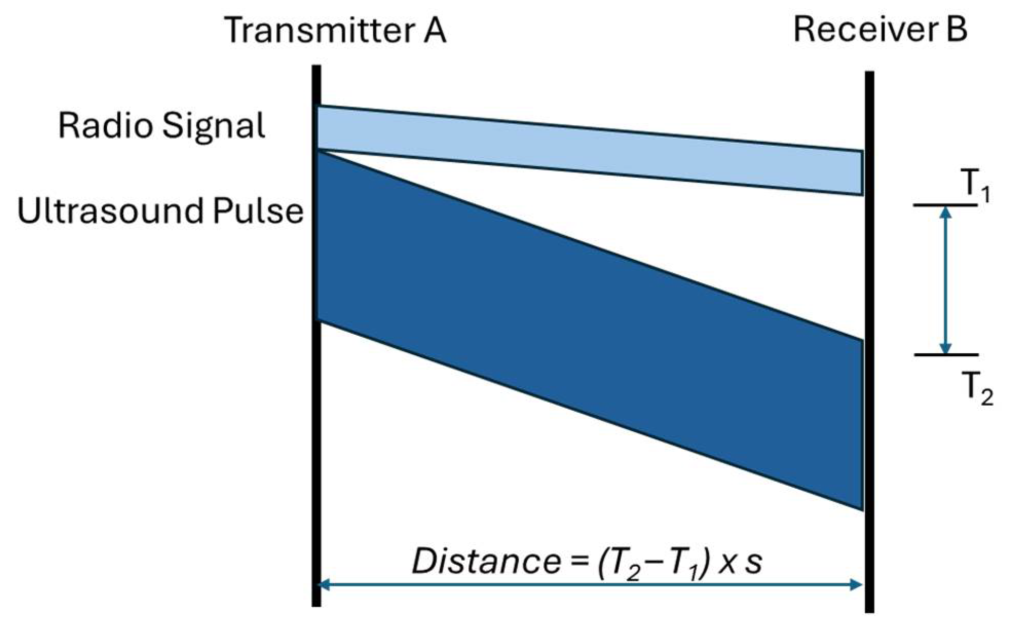
An interesting approach still based on time is the is known as time difference of arrival (TDoA). In this case, the emitter node transmits two signals that have different speeds, namely a radio frequency signal and an ultrasound pulse, as represented in Figure 2. Receivers infer the distance from the differences between the instant of ultrasound signal arrival T₂ and that of radio signal arrival T₁.

The big advantage of the TDoA method over simple measurements of time of arrival is the lack of synchronization requirements since, in this case, it does not need to be absolute.

3.4. Angle-Based

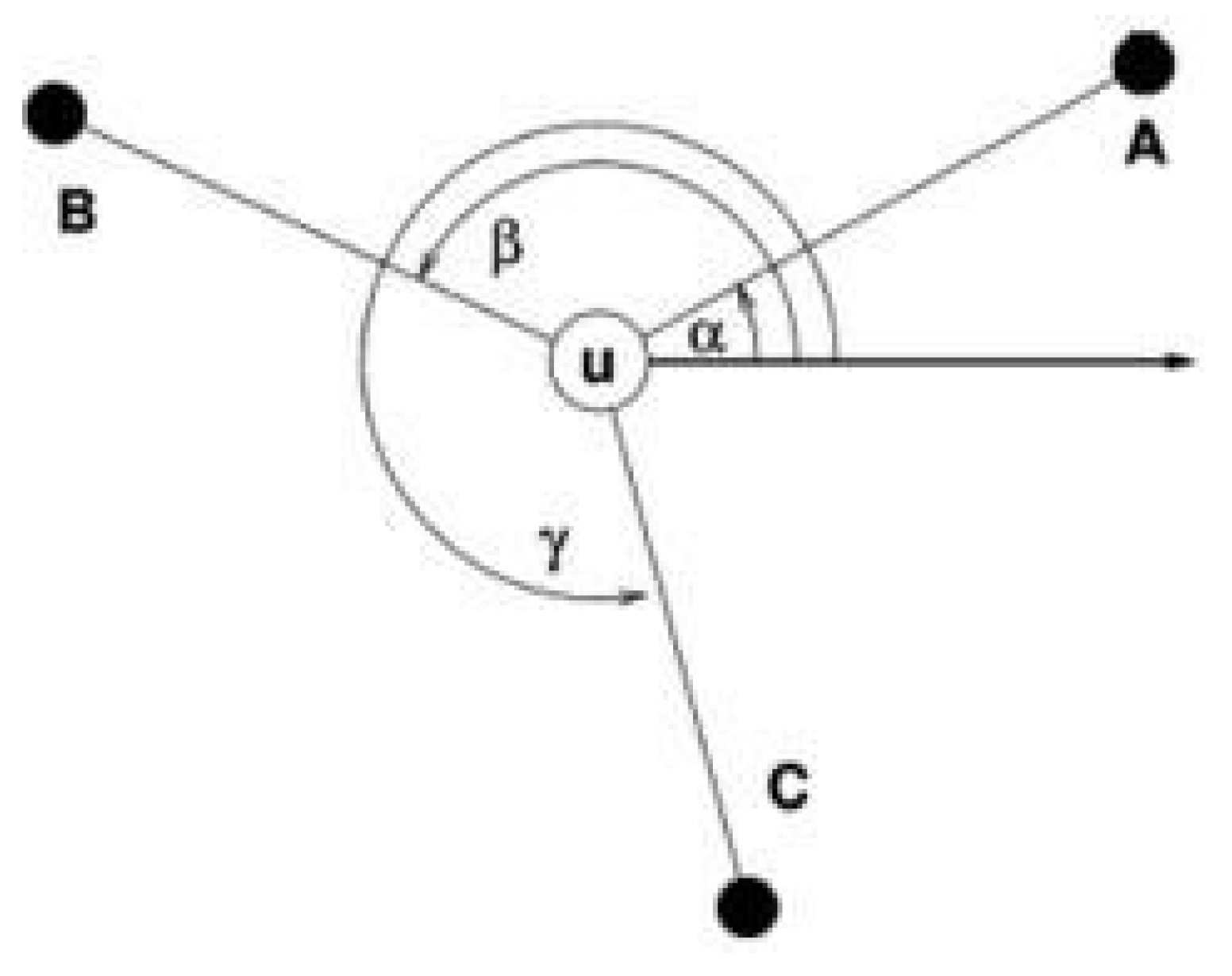
In this approach, the direction joining the anchor and target is often referred to as the direction of arrival, usually known as the Angle of Arrival (AoA). It is useful for the measurement node to exploit directional antennas [4] to estimate the Angle of Arrival, which is computed based on an angle system. In Figure 3, an example with three Anchor nodes (A, B, C) is presented. Once a target node has fixed a reference, it can measure the angles (α, β, γ) from radio signals coming from each Anchor, so the estimated position is given by the intersection u of the three rays originated by each Anchor. The advantage of Angle-of-Arrival-based methods is that they do not require flight time estimation (and consequently not even synchronizations).

3.5. Received Signal Strength Indicator—RSSI

The term received signal strength indicator, or RSSI, refers to a numerical value that indicates the power of a received signal, thanks to which it is possible to estimate the distance from the station that transmitted it. This parameter is measured in dBm, or decibels-milliwatts, which is the unit of measure used to indicate a power ratio expressed in decibels (dB) with reference to a milliwatt (mW). In

Table 1. RSSI values relative to received signal power.

Power (dBm)	Power (dBW)	Power (Watt)
−100	−130	0.1 pW
−90	−120	1 pW
−80	−110	10 pW
−70	−100	100 pW
−60	−90	1 nW
−50	−80	10 nW
−40	−70	100 nW
−30	−60	1 µW
−20	−50	10 µW
−10	−40	100 µW
1	−31	794 µW
0	−30	1 W

, a table associating typical RSSI values with received signal strengths is shown. The higher the RSSI value, the stronger the received signal.

It is assumed that the received power follows the polynomial decay model, typical of the Friis’ model [15]. This power is, in fact, assumed to depend on the transmitted power, on the path loss constants, and on the distance between the source and the receiver. The Friis equation evaluates the power P_R received from a transmitter placed at distance d:

$$P_R={\displaystyle \frac{P_T{G}_T{G}_R{\lambda }^2}{\left(4\mathrm{\pi }\right)2dn}}$$

(1)

where the following apply:

P_R: transmitted signal strength in watts;

G_R: receiving antenna gain;

G_T: gain of the transmitting antenna;

λ: signal wavelength; d: distance in meters;

n: propagation constant of the signal, also called propagation exponent, dependent on the environment.

RSSI can be then calculated by converting the power from Watts to dBm:

$$RSSI\left[\mathrm{dBm}\right]=10{\log }_{10}P\left[\mathrm{mW}\right]$$

(2)

There is a different expression of RSSI, based on the beacon distance formula:

$$RSSI=-10n\log d+A$$

(3)

where the following apply:

A: The RSSI value (in dBm) at a reference distance, typically 1 m from the beacon. This value is often provided by the beacon manufacturer and represents the signal strength at a known distance.

RSSI: The current received signal strength indicator value (in dBm) measured by the receiver. This value indicates the strength of the beacon’s signal at the receiver’s location.

n: The path-loss exponent, which accounts for the environment’s effect on signal propagation. The value of N typically ranges between 2 (representing free space) and 4 (representing indoor environments with obstacles such as walls and furniture).

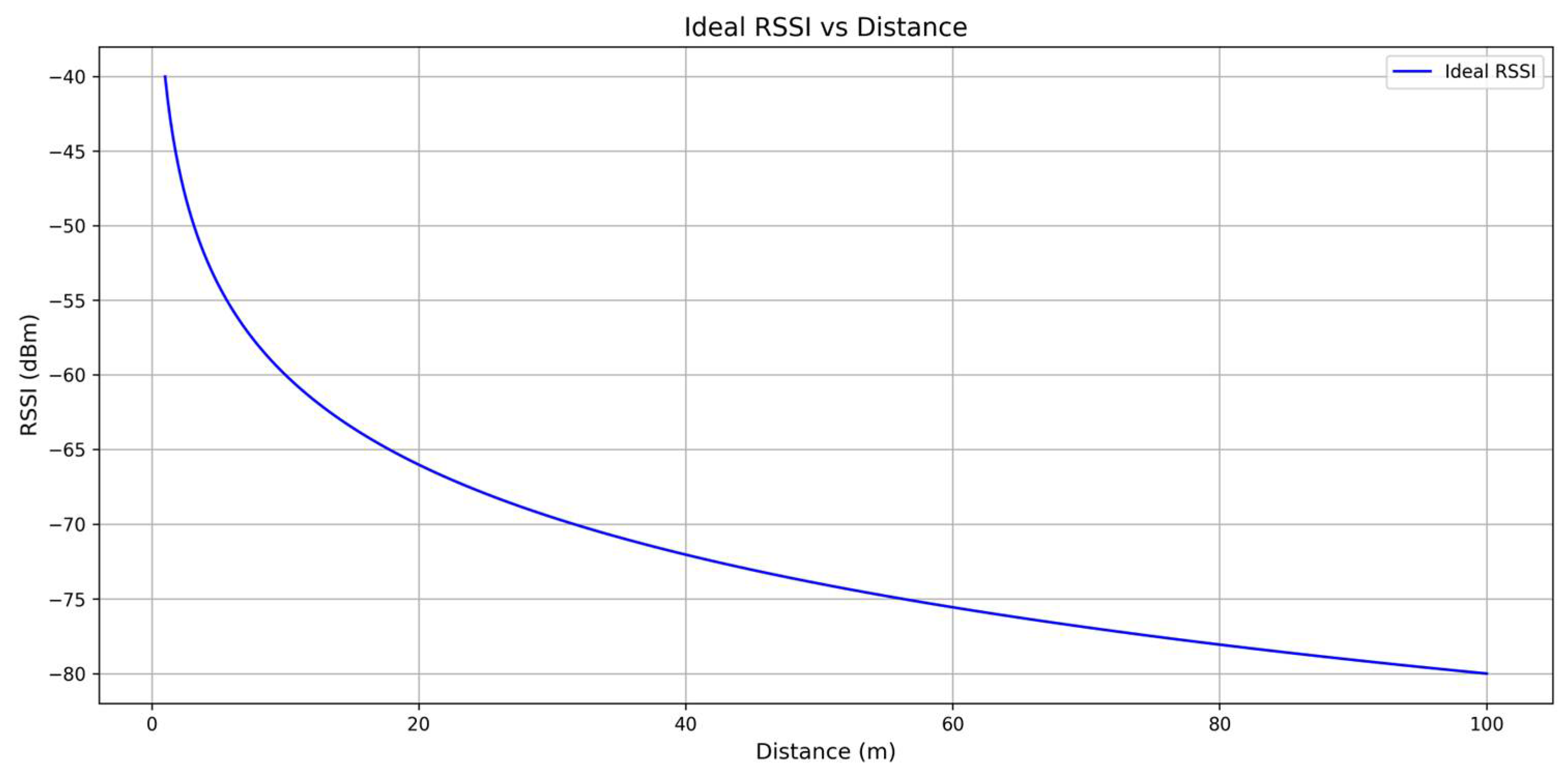
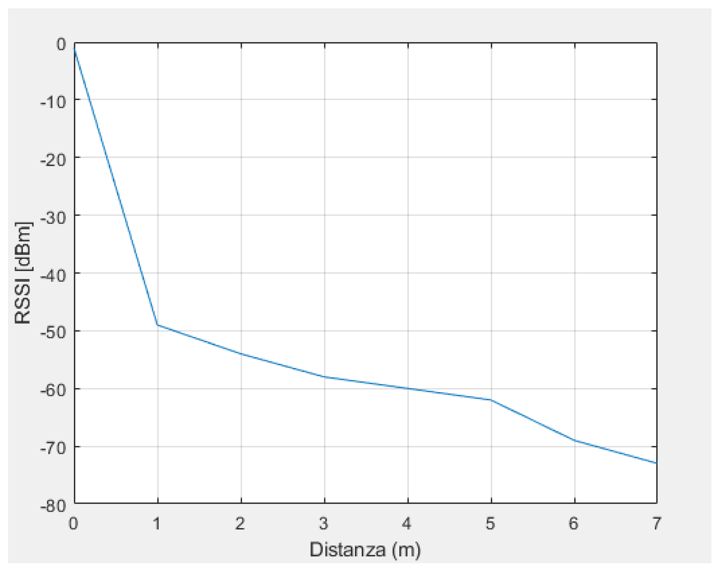
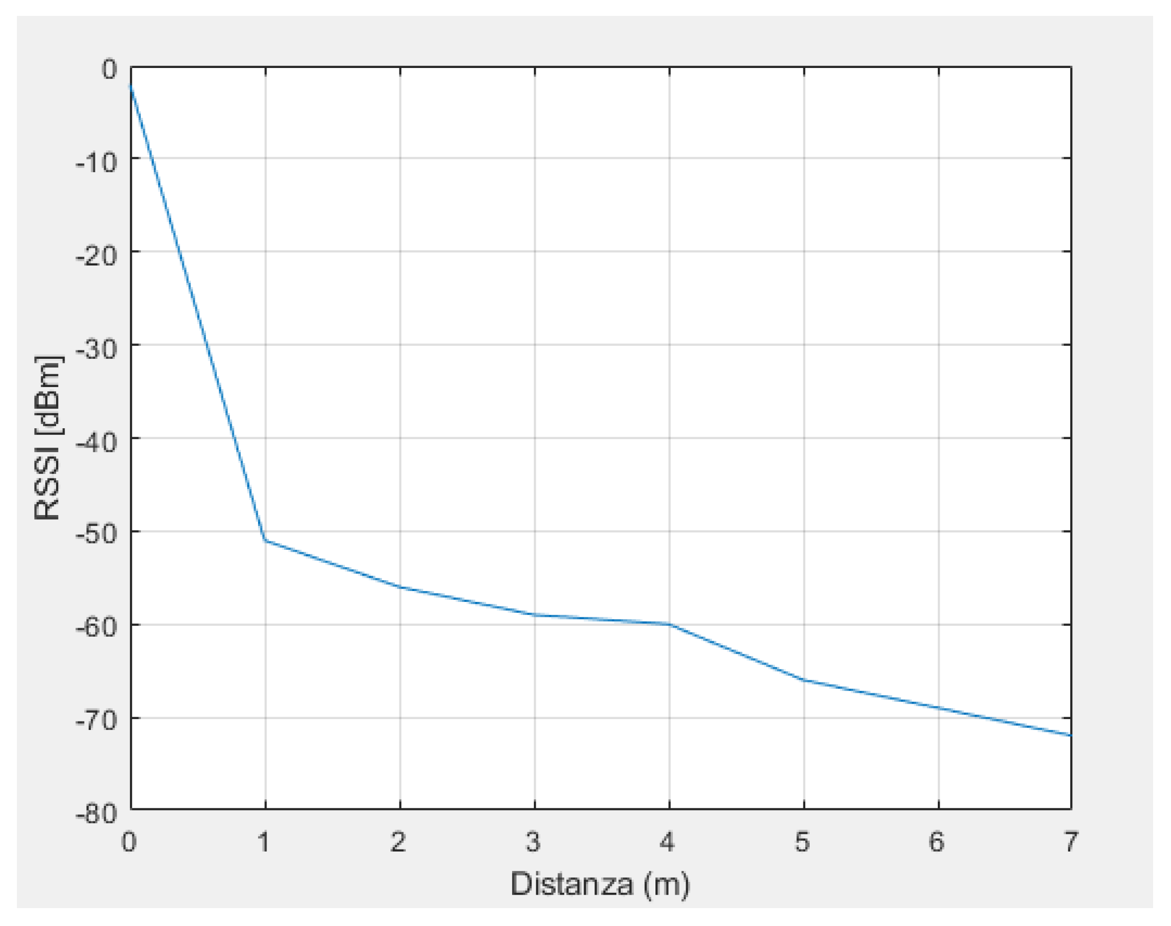
Figure 4 shows the ideal trend [20] of the RSSI in the open environment (A = −40 dBm and n = 2). The distance is then

$$d={\displaystyle \frac{{10}^{(A-RSSI)}}{10\times n}}$$

(4)

With the use of this final formula, the distance between two nodes can be determined given the RSSI value and the parameters A and n.

Since the RSSI can be used without additional hardware in any devices, many research activities in recent years have focused on the use of this index for localization. Efforts were initially concentrated on the analysis of this indicator and on a better understanding of the causes of its very strong localization variability. Being widely used in the localization domain, this parameter is exploited for the purpose of this work.

4. Localization Algorithms

Once the distances to the fixed nodes have been determined, the target can determine its position, which is performed in the so-called positioning phase.

In this section, the range-based and Anchor-based algorithms are used, so it is necessary to have the presence of reference nodes whose position is known in advance. Also, as mentioned earlier, the RSSI is used as the distance estimation method, i.e., the target node converts the RSSI value ascribed to each Anchor into a distance, thus estimating its own distance from the reference nodes. The problem will be tackled with a two-dimensional approach, i.e., the position of the localizing node will be understood as completely known once two of its three spatial components are known. This simplification is legitimated by the type of domain that a localization system can cover. In fact, not only is the two-dimensional position compatible with all the cases of practical interest that the new frontier of indoor localization presents, but it is also relatively simple to extend most of the results to an actual three-dimensional case.

4.1. Min–Max

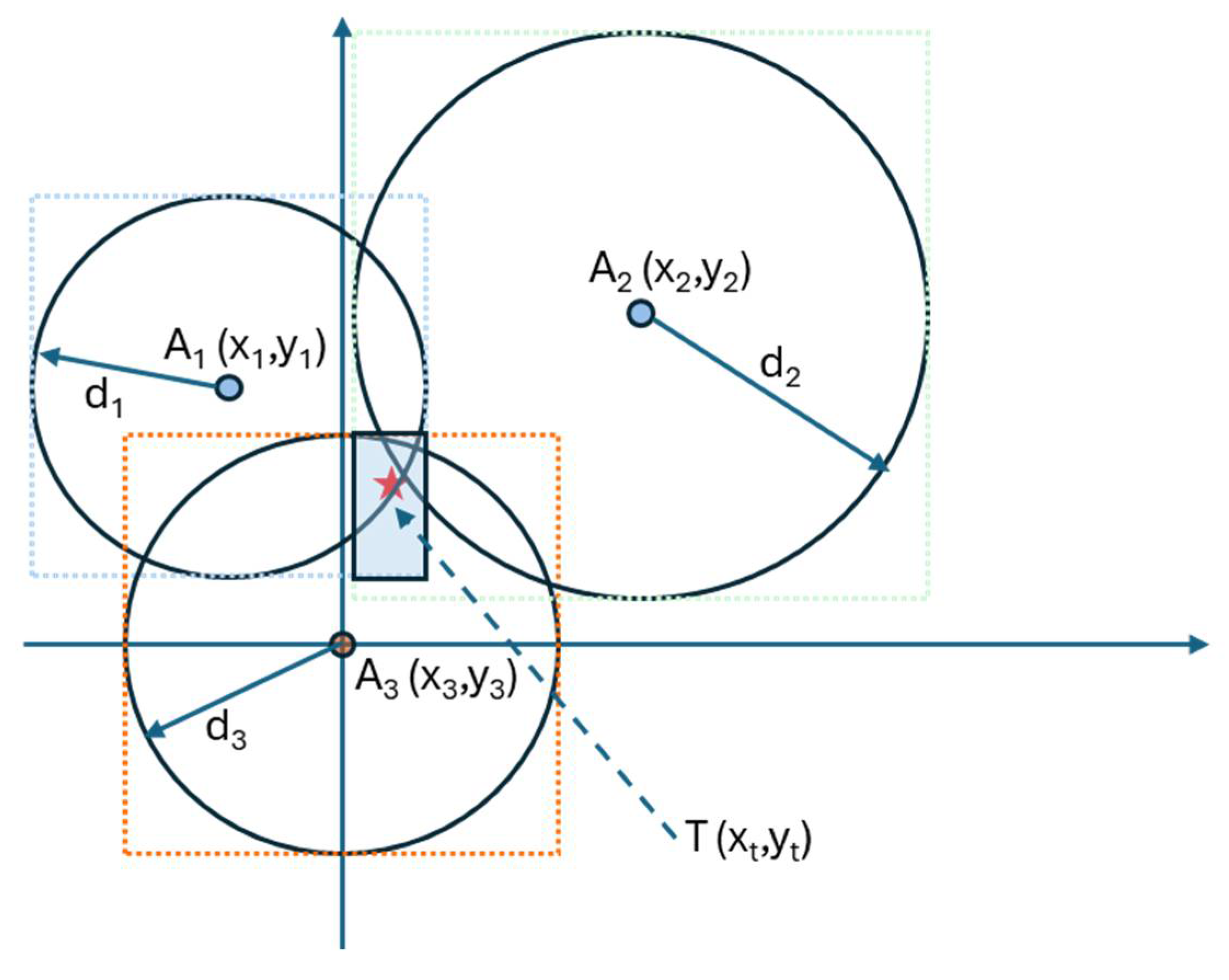
Min–Max is a popular localization algorithm whose success is mainly due to its extreme simplicity of implementation. A number N of fixed Anchor nodes is positioned at known coordinates (x_i,y_i), where I = 1, 2, …, N. A target T is situated at (x_t,y_t), which needs to be determined. Once the target collects RSSI measurements and convert them into distances d_i, squares are constructed for each Anchor by drawing two horizontal lines and two vertical lines around each reference node so that the side of this square is equal to the double of distance di, as showed in Figure 5. The intersection of these squares determines another quadrilateral whose coordinates can be calculated as follows:

$$\begin{gathered} V_1=\left[max\left(x_i-d_i\right),max\left(y_i-d_i\right)\right] \\ {V}_2=\left[max\left(x_i-d_i\right),min\left(y_i+d_i\right)\right] \\ {V}_3=\left[min\left(x_i+d_i\right),min\left(y_i+d_i\right)\right] \\ {V}_4=\left[min\left(x_i+d_i\right),max\left(y_i-d_i\right)\right] \end{gathered}$$

(5)

Finally, the position estimated is calculated at the center of the intersecting quadrilateral as follows:

$$\begin{gathered} x_{est}={\displaystyle \frac{\left[min\left(x_i+d_i\right),max\left(x_i-d_i\right)\right]}{2}} \\ {y}_{est}={\displaystyle \frac{\left[min\left(y_i+d_i\right),max\left(y_i-d_i\right)\right]}{2}} \end{gathered}$$

(6)

Hence, the smaller the area of the intersection rectangle, the higher the localization accuracy.

4.2. Trilateration

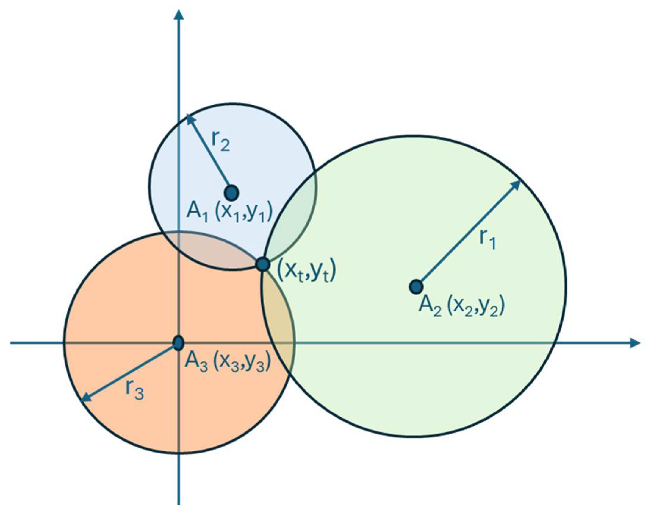
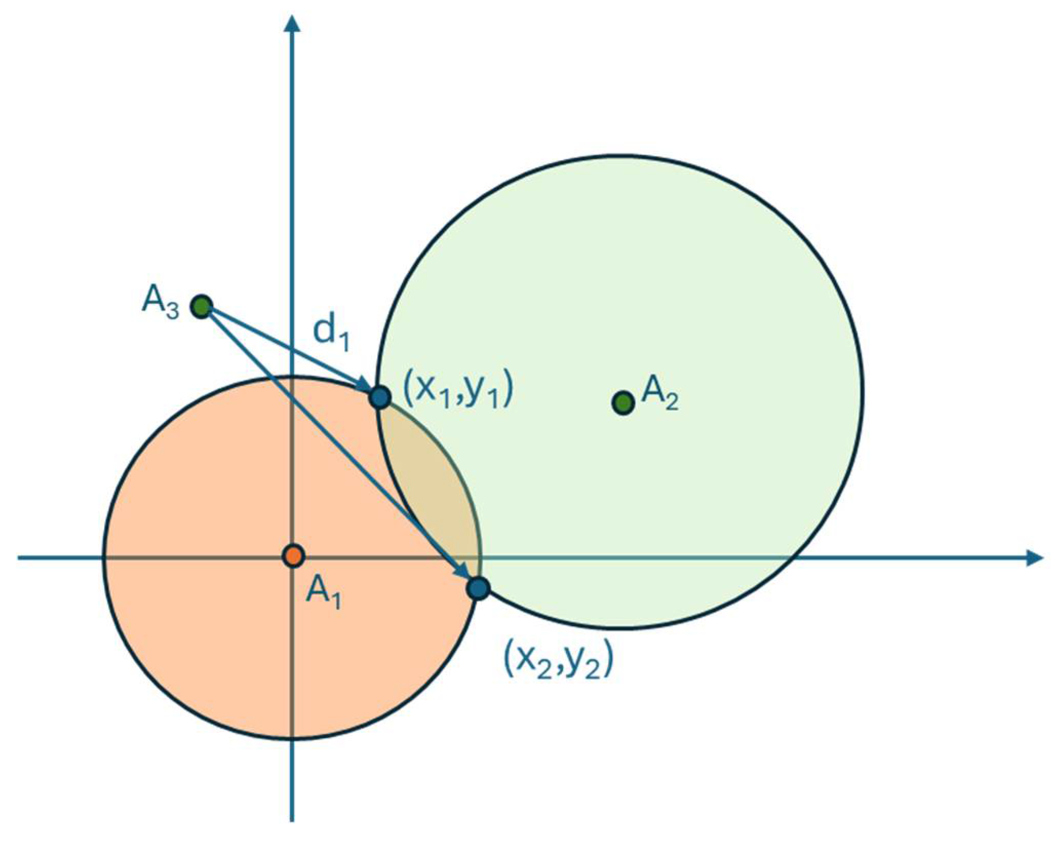
Trilateration, or multi-lateration as it is more properly called in the general case where N references are available, is an algorithm that estimates the position of the target based on geometric properties.

As before, RSSI measurements are collected and converted to distances d_i, at which point the target position is obtained as the result of a non-linear system that defines a circumference for each Anchor:

(x − x_i)² + (y − y_i)² = d_i²

(7)

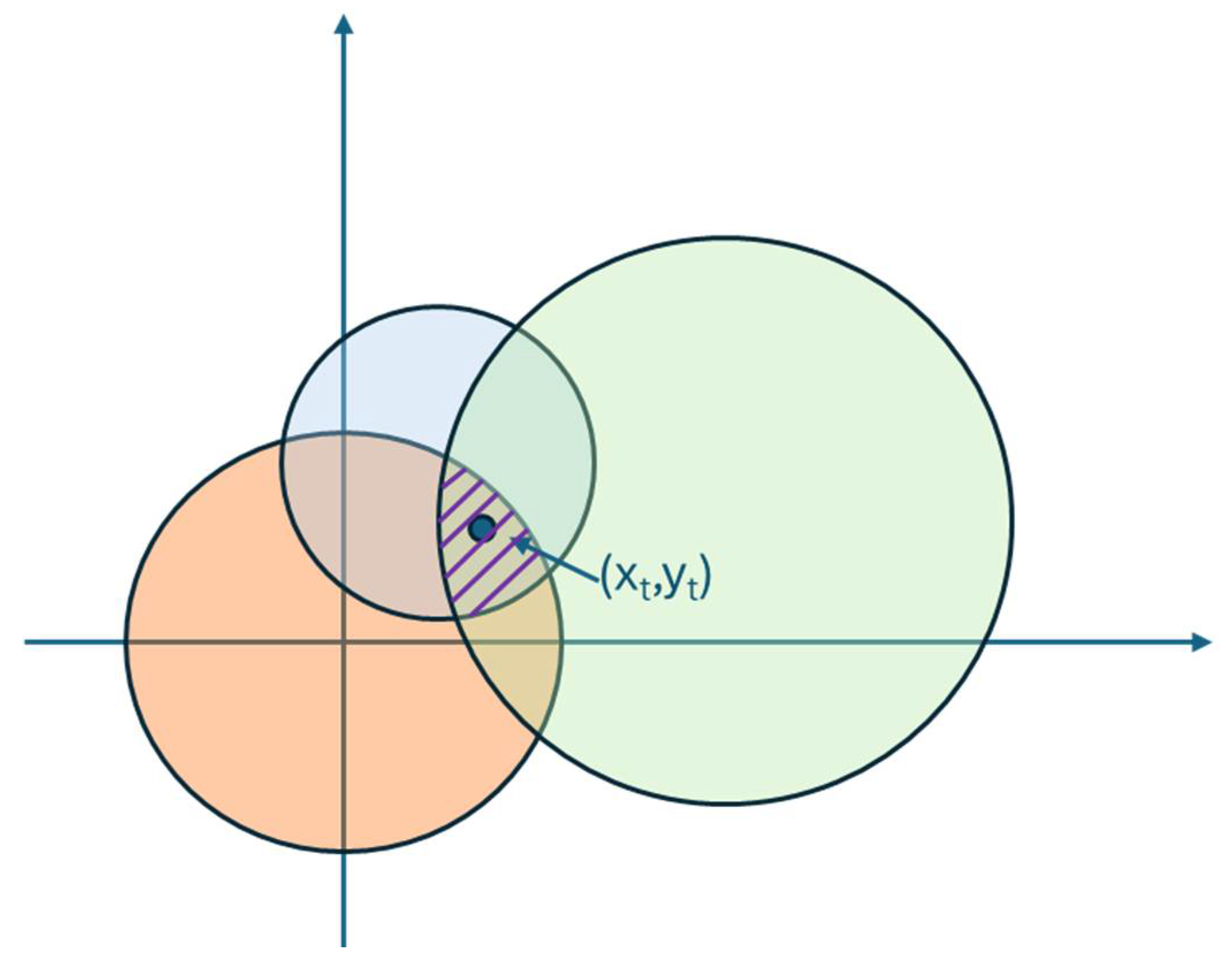
where d_i is the radius of the circumferences and (x_i, y_i) the center of the circumferences, as shown in Figure 6. The intersection of the circumferences locates the position of the target. In case of three Anchors, this results in the following system of equations:

(x − x₂)² + (y − y₂)² = d₁²

(x − x₂)² + (y − y₂)² = d₂²

(x − x₂)² + (y − y₂)² = d₃²

(8)

However, because of inevitable measurement errors in the distance estimation, the three-Anchor trilateration system can only be solved exactly theoretically. This is because noise perturbs the three circles, making it impossible for them to intersect exactly, which means that the estimated target position is almost never obtained as the intersection of circumferences, but falls inside an estimated area represented with a grid in Figure 7.

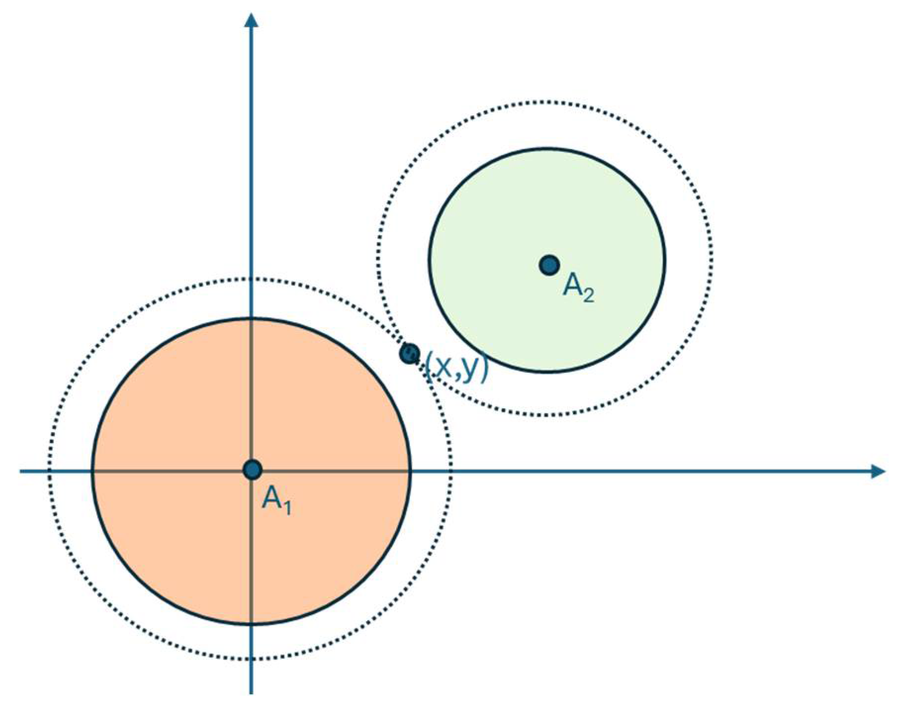
4.3. Alternative Trilateration Method

To address the issue presented above, one can reduce the number of steps in the traditional method by drawing inspiration from the proposal in [21]. The steps that will be described are performed iteratively for each pair of Anchor nodes.

• Given a pair of nodes and their circumferences, if the point of intersection is unique, it is saved;
• If the two circumferences do not intersect, like in Figure 8, the radii of each circumference are increased proportionally so that they intersect at a single point (the radius is increased until to the dotted lines);
• If instead the two circumferences intersect in two points, like in Figure 9, the one that is closest to a third Anchor node is considered.

At the end of this procedure, iterated for each node pair, the average of the coordinates is computed, which corresponds to the estimated position of the target node.

4.4. Triangulation

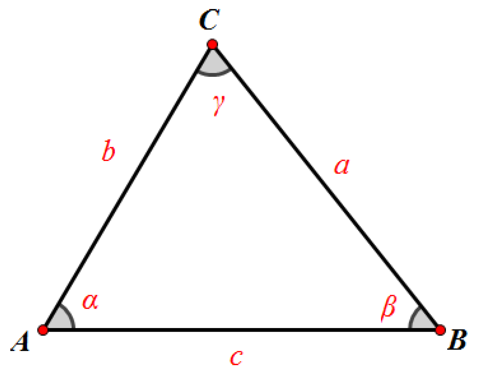
Triangulation is a localization algorithm for determining the position of a point by measuring the angles at the base of a triangle that has two points of known coordinates as its base vertices and a vertex of unknown coordinates as its top vertex. Trigonometric formulas are used to calculate the target coordinates.

Assuming we know the coordinates of Anchor nodes A and B, as represented in Figure 10, and that all nodes are at the same height, the distance c between the two reference nodes is known.

Once the distances of the target node from the reference nodes are estimated, as a and b are also known, the coordinates of point C can be derived.

Starting from the Cosine Theorem (or Carnot’s Theorem) [15], cos(α) is calculated as follows:

$$\cos (\alpha )={\displaystyle \frac{b^2+c^2-a^2}{2bc}}$$

$${\sin }^2\left(\alpha \right)+{\mathrm{c}\mathrm{o}\mathrm{s}}^2\left(\alpha \right)=1$$

$$\sin \left(\alpha \right)=\sqrt{1-{\cos }^2\left(\alpha \right)}$$

(9)

If we set point A as the origin of the reference system, i.e., coordinates (0,0), then point C has the following coordinates:

$$C=(b\cos \left(\alpha \right),b\sin \left(\alpha \right))$$

(10)

It should be specified that the triangulation method is not always successful. In particular, if the target node is on the segment joining the two Anchor nodes, the algorithm does not provide any position estimates because no triangle is formed, and therefore, the trigonometric formulas cannot be applied.

In addition, unlike the previously described algorithms that were based on at least three Anchor nodes, for triangulation, only two nodes are needed, but this results in a lower accuracy in position estimation.

5. Testbed Implementation

The main objective of this work is to implement a system that uses WSN infrastructure to measure located mobile objects using RSSI. The application involves scattering a given number of fixed nodes over an observation region or area of interest; these nodes work together to determine where the mobile node in the network will be located.

The mobile node, designated as the object to be monitored, moves within the monitored region and communicates with the fixed nodes in the network, allowing the system to stabilize the node’s position with reasonable accuracy. The interaction between the mobile node and fixed nodes is crucial to measuring mutual distances (based on the RSSI index), which is then used to determine the position of the mobile node using location algorithms. Then, the different algorithms are compared to determine which one is more efficient and accurate in estimating distance.

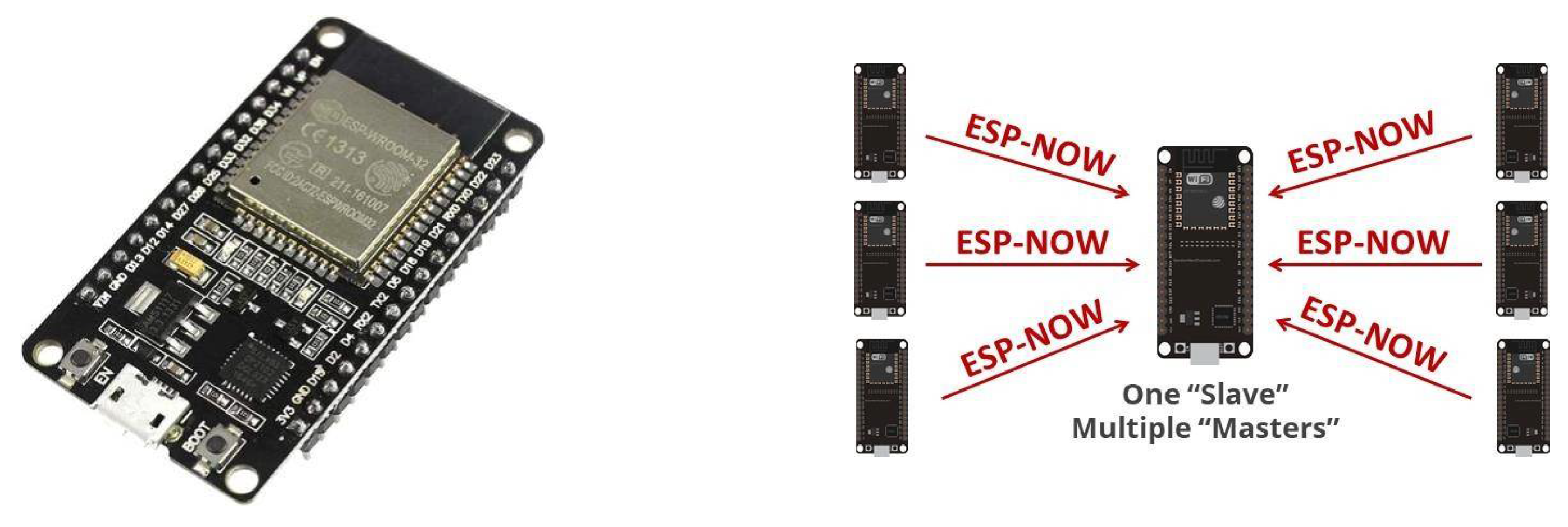
The system nodes consist of the ESP32 module DevKitMv1 developed by Espressif Systems, a semiconductors company located in 690 Bibo Road, Shanghai, Shanghai 201203, CN. This module is depicted on left side of Figure 11, and it represents an evolution of the ESP8266 module, widely used in the IoT field.ESP32 is a low-cost, low-power microcontroller series based on the ESP-WROOM-32 chip with integrated Wi-Fi and dual-mode Bluetooth and uses a 32-bit dual-core Tensilica Xtensa LX6 microprocessor.

MCU Specifications:

Tensilica LX6 dual core 32-bit microprocessor;

Working frequency settable between 80 MHz and 240 MHz;

ROM: 448 KB for booting and CPU;

SRAM: 520 KB for data and instructions;

RTC slow and fast SRAM: 16 KB for data storage and coprocessor access during deep-sleep mode.

WiFi: 802.11 b/g/n/d/e/i/k/r up to 150 Mbps;

Bluetooth v4.2 BR/EDR and BLE (Bluetooth low-energy) support.

The ESP32 devices have been programmed using the Arduino IDE version 1.8.19, a cross-platform application written in Java, provided with an easy-to-use and intuitive C/C++ software library and derived from the IDE created for the processing programming language.

It should be specified that for the ESP-WROOM-32 chip, the output power at the antenna reaches 20.5 dBm; this is because Equation (4), on which the calculation of the RSSI is based, takes into account the power of the signal transmitted by the emitter (in Watts). All the source codes implemented to perform the measurements described in the following sections is available on github https://github.com/maudarie/sensorLocalization (accessed on 1 April 2025).

5.1. Communication Protocol

To let the target node be able to collect RSSI values for each reference node, a wireless connection between the devices must be established. Once the connection has been established, the target receives simple data packets (i.e., signals) from the reference nodes, and every time it receives a packet, RSSI is calculated based on the number of transmission errors detected in the newly received packet, since a higher number of errors is expected for lower received powers.

The ESP-Now communication protocol (available at https://github.com/espressif/esp-now, accessed on 1 April 2025), also developed by Espressif Systems, was used to implement the sensor network and enable the devices present to communicate with each other in order to reduce power consumption during wireless communication. Esp-Now activates a peer-to-peer transmission between ESP family devices, with a power consumption lower than the classic Wi-Fi communication.

It uses the integrated Wi-Fi module, so it always uses the 2.4 GHz band, but in this case, it does not make a classic connection to the Wi-Fi Access Point and it does not interfere with normal home wireless communications.

Energy saving is not achieved by decreasing the transmission power but by simplifying and reducing the connection and communication time.

The transfer of a packet can have a maximum size of 250 bytes. It is not suitable for the transmission of high rates, but it is sufficient for the transfer of small data, typical of IOT applications. Data can be transmitted unidirectionally or bidirectionally, single-duplex or full-duplex, and be encrypted.

The communication mode on the right of Figure 11 foresees a board that is the target acting as receiver (or Slave) and several boards acting as emitters (or Master). Note that there are no “emitter/master” and “receiver/slave” components in the ESP-Now documentation. Each board can be an emitter or a receiver. However, to keep things clear, both these terms are used to differentiate their role. The sender board receives a confirmation message indicating whether the message has been delivered correctly or not, while the receiver board receives messages from all the senders and is able to identify which board sent the message. Since the target is able to identify which device sent a packet, it can associate each device with an RSSI value and thus establish distances from the devices.

As seen, we need to model the radio channel of our environment and then derive the parameters A and n so that Equation (4) can be applied.

The methodology used to derive these parameters is based on an empirical method, i.e., the observation of data. Parameter A is the power of the received signal, in dBm, at the reference distance of 1 m. To establish how much it is worth, the value it assumes is observed by placing two devices at the exact distance of 1 m and making an average of more values, as shown in Table 1 and

Table 2. Propagation exponent.

Environment	Path Loss Exponent (n)
Free space	2
Urban area cellular radio	2.7 to 3.5
Shadowed urban cellular radio	3 to 5
Inside a building–line of sight	1.6 to 1.8
Obstructed in building	4 to 6
Obstructed in factory	2 to 3

. The functions of the program loaded on the device carrying out these measurements reported that in an indoor environment, this parameter assumes the average value of A = −49 dBm, while in an outdoor environment, the value is A = −51 dBm.

Parameter n, as already shown, is the so-called signal propagation constant; it indicates the reduction in the power density of an electromagnetic wave as it propagates in space. This value is usually between 2 and 4, as shown in Table 2, where 2 indicates propagation in free space, 4 indicates lossy environments, and for the case of complete specular reflection (in some environments, such as buildings, stadiums, and other indoor environments), it can reach values between 4 and 6.

The choice of the value was made by observing the distance values obtained for different values of n. In particular, the experimentation phase showed that in an indoor environment, the use of the value n = 1.6, as also shown in the figure above, is very adequate because it provides RSSI values very close to the ideal ones.

Instead, for the outdoor environment, the value n = 1.9 was chosen for the same reasons.

Once these parameters have been determined and the distances have been calculated by exploiting the RSSI index, the localization phase comes into play, and dedicated algorithms can be applied.

5.2. Localization

First, the target distances from the Anchor nodes are estimated. To do this, three reference nodes were set with the following coordinates, (0;0), (5;0), and (0;5), where each single unit in the reference system corresponds to 1 m. The target device was then positioned within the area delimited by the Anchor nodes. (In the case of triangulation, the device at position (0;5) is not present for obvious reasons).

On each reference device, the first code was executed to continuously send packets towards the target node. The target device executes the code that first collects the RSSI values for each device, with correct parameters A and n. It then applies Equation (4) to estimate the distance between the target node and each reference node.

Next, the program performs the positioning phase; that is, it applies the localization algorithms and estimates the position of the target node. The Min–Max, triangulation, and trilateration source codes are all available on github.

6. Experimental Results

In this section, some considerations on the experimental results are provided, starting with the precision of the distance estimation carried out thanks to the RSSI index and how variable this can be under certain conditions. Then, in the following step, the selected location algorithms are compared, and it is determined which of the three is more accurate in the estimation of the position. Table 1 and Table 2 show RSSI measurements associated with multiple distances, both indoor and outdoor, calculated by placing two devices (one configured as the target and the other as the Anchor) at different distances.

Measurements were made in different environments to test whether, and how, the relationship between RSSI and distance changes depending on the environment in which the radio signal propagates.

The values obtained are the result of the average carried out on 25 samples because it has been observed that using fewer values makes the measurement too variable. Moreover, each time the average of the RSSI index is made on a smaller number of samples, it results in something too different from the previous calculation. Therefore, this number of samples can be considered sufficient to determine the RSSI value of the communication between two nodes in a WSN.

It is also preferred to use the standard deviation [2] as an index of variability because, in the presence of a fairly high number of measurements, it best represents the absolute error and is therefore of fundamental importance in order to correctly determine the magnitude of the fluctuations found in the measurements.

6.1. Indoor Environment

Table 3. RSSI in indoor environment.

d (m)	RSSI (dBm)	σ
0	−1	2.132
1	−49	0.748
2	−54	0.787
3	−58	0.810
4	−60	0.911
5	−62	2.328
6	−69	2.484
7	−73	3.801

shows the values obtained from the measurements made indoors. Observing the reported RSSI values, it can be observed that these reflect quite well the ideal trend reported in Figure 5, and it is possible to appreciate even more the similarity between the real and the ideal decreasing exponential trend in Figure 12.

As the distance between the devices increases, the RSSI increases negatively, meaning that the signal strength reaching the receiver tends to decrease as the devices move further apart, as is normal. It is also good to note that the standard deviation increases when the distance increases, in agreement with the fact that the measurements taken will be less accurate as the distance increases. It was expected that the data obtained were not perfectly equal to the ideal ones, precisely because the signal of radio communication is influenced by the environment in which it propagates and by the effects mentioned earlier, such as shadowing, multipath, etc.

6.2. Outdoor Environment

Table 4. RSSI in outdoor environment.

d (m)	RSSI (dBm)	σ
0	−2	0.898
1	−51	0.644
2	−56	0.871
3	−59	1.358
4	−60	1.480
5	−66	2.013
6	−69	2.135
7	−72	2.259

shows instead the values obtained outdoors with no obstacles between the devices and in the line of sight. In this case, the RSSI index does not differ much from that of the previous case; it continues to reflect the ideal trend, as reported in Figure 13. The difference can be seen in the standard deviation, which tends to have smaller values. This reflects the fact that the effects of reflections and environmental effects are less pronounced, as a smaller standard deviation value means that there is less variability in the RSSI calculation, i.e., the individual measurements are closer to the mean value.

Therefore, it can be said that the received signal strength indicator is reliable and usable for estimating distances; moreover, it is more suitable for outdoor environments as expected. If it was not usable, the localization algorithms would work with false values, and the results obtained would be meaningless.

6.3. Comparison of Algorithms

Table 5. Position estimates.

Real Coordinates		Estimated Coordinates		Estimation Error		Euclidean Distance Error	Algorithm
x	y	x	y	x	y	D
2	0	1.53	0.74	0.47	0.74	0.87	Min–Max
		null	null	null	null		Triangulation
		2.44	0.65	0.44	0.65	0.78	Trilateration
1.5	1.5	1.91	1.89	0.41	0.39	0.56	Min–Max
		2.11	2.37	0.61	0.87	1.06	Triangulation
		1.86	2.02	0.36	0.52	0.63	Trilateration
3	3	3.81	3.32	0.81	0.32	0.87	Min–Max
		4.23	3.74	1.23	0.74	1.43	Triangulation
		3.41	2.87	0.41	0.13	0.43	Trilateration
3.5	4	3.26	3.54	0.24	0.46	0.51	Min–Max
		4.51	3.35	1.01	0.65	1.20	Triangulation
		3.97	4.36	0.47	0.36	0.59	Trilateration

below shows the results obtained by the algorithms applied outdoors as RSSI reported many outliers indoors. The position of the target is calculated as an average of five measurements, and the Euclidean distance error from the real point is provided in the last column of Table 3.

The algorithm that performs best in this case is trilateration. This can be observed from the distance error, which is lower for almost every set of coordinates of the target node.

It was not easy to predict that it would be the most accurate algorithm because it is true that it is the most complex, and in some cases, it performs operations that approximate the values in the best way (such as the proportional increase in the radii), but at the same time, it is also the one with the highest computational cost, so the estimation error can propagate and increase for each operation performed, compromising the localization.

The least accurate algorithm is triangulation; it has quite high estimation errors. This is due to the fact it uses only two reference nodes to calculate the position compared to the other algorithms that make use of three nodes. In general, it can be said that the Min–Max algorithm and the trilateration algorithm provide relatively good results by calculating sets of coordinates that reflect the position of the nodes that are reliable enough.

Note that the estimated coordinates from triangulation are null in the case where the target’s coordinates are (2,0). This is true for any coordinate where the target node is on a straight line connecting the two reference nodes. This results from the absence of a triangle, making it unable to use the trigonometric formulas shown in Section 4.

7. Conclusions

This paper explores the role of received signal strength indicator (RSSI) in the localization of objects within a wireless sensor network (WSN). A real-world WSN testbed is implemented with low-cost devices, making this solution not only accessible but also scalable for a variety of real-world applications. A comprehensive comparison of three widely used RSSI-based localization techniques—Min–Max, triangulation, and trilateration—provides a detailed analysis of their performance, strengths, and limitations in real-world scenarios. This comparison serves as a valuable guide for practitioners seeking to select the most appropriate localization technique for their specific needs and network environments.

The experimental results emphasize the critical need for accurate RSSI values to improve the precision of object localization in WSNs.

While this work lays the groundwork for deploying localization techniques in sensor networks, it does not introduce novel hybrid approaches nor does it address some of the key challenges in improving RSSI accuracy. Looking forward, there are several potential directions for future work. One promising avenue is the integration of hybrid techniques that combine RSSI with other sensor modalities, such as time of flight (ToF) or Angle of Arrival (AoA), to enhance localization accuracy. Techniques such as machine learning-based models could also be explored to compensate for the noise and variability inherent in RSSI measurements, further improving performance. Additionally, the adoption of advanced calibration techniques and error correction algorithms, such as Kalman filtering or particle filtering, could address some of the issues related to signal interference and multipath effects. Other existing approaches like network-wide cooperative solutions are instead more suitable for large-scale networks.