1. Introduction
Finding an available on-street parking place has been considered as an old and noticeable challenge in large size cities. Drivers looking for vacant parking places can negatively impact traffic conditions and the environment (e.g., pollution and automotive fuel consumption) [
1,
2]. Studies of cruising in several congested downtowns between 1927 and 2001 showed that the average time to find a curb space ranged between 3.5 and 14 min and also between 8 and 74 percent of the traffic was cruising for parking [
3]. Results of a recent study [
4] also indicates that between 9 and 56 percent of the traffic is cruising for parking and the average search time is around 6.03 min.
The combination of Artificial Intelligence (AI) technologies with the Internet of Things (IoT) infrastructure refers to Artificial Intelligence of Things (AIoT). AIoT can achieve more efficient and autonomous IoT operations, improve human-machine interactions and enhance data management and analytics [
5]. In a smart parking, AIoT can help drivers to save searching time and automotive fuel by predicting short-term parking place availability.
In this work, we consider parking segment prediction rather than an individual on-street parking place. Where a street (or part of that) with the possibility of car park is considered as a segment. We decided to consider the parking segment prediction because predicting situation (i.e., vacant or occupied) of an individual on-street parking place is technically very difficult, inaccurate and even not possible. In addition, the drivers are usually willing to know parking availability of segment rather than an individual parking place on a street.
Machine Learning and Neural Network-based (MLNN) algorithms can be applied to large datasets of different applications in order to extract relevant information and for making predictions. However, the results of the algorithms may vary depending upon the datasets and application being used. Therefore, determining the most suitable algorithm for specific datasets and application can be considered as a key advantage.
In order to find the the most suitable MLNN algorithm for predicting parking segment availability, we compare several well-known MLNN algorithms (e.g., K-Nearest Neighbors (KNN), Decision Tree (DT), Random Forest (RF), and Voting Classifier) based on a real parking datasets. The datasets that we use contain around five millions records of the measured parking availability in San Francisco.
We implement the algorithms using Scikit-Learn and Pytorch and compare them considering the well-known evaluation metrics: Precision, Recall, F1-Score, and Accuracy.
In addition, we propose a recommendation system including an algorithm to predict parking segment availability (i.e., utilizing the selected MLNN model) in a desirable time interval (e.g., 30 min later) and, in case of unavailability, suggest alternative segments.
To our knowledge, there are quite a few works (see Related Work section) which tried to evaluate performance of different MLNN algorithms for predicting car park place availability. Different from these works, this paper evaluates a wider range of MLNN algorithms including a large number of various combinations of them (i.e., more than 50 combinations). We also consider some additional metrics that previous works have not considered such as execution time of the algorithms and the walk forward validation technique (instead of k fold cross validation) as well as the three-level parking availability technique to improve performance of our recommendation system.
Our main contributions are listed below with respect to the main objective of predicting the availability of parking spaces:
performance evaluation of various MLNN algorithms (e.g., KNN, RF and DT);
performance evaluation of the Ensemble Learning approaches (i.e., with various configurations)
comparing performance of different MLNN and Ensemble Learning to find the best one for the problem of predicting parking segment availability;
introducing and simulating our recommendation system to offer the most suitable parking segment to drivers based on their requested destination and prediction time.
This paper is organized as follows.
Section 2 introduces the related work. In
Section 3, we describe our use case and the recommendation system.
Section 4 briefly presents the MLNN algorithms under study in this paper. In
Section 5, we implement and evaluate the performance of different MLNN algorithms and their combination (i.e., Ensemble Learning) as well as the proposed recommendation system. In
Section 6, we will have a discussion and, finally,
Section 7 concludes our work.
2. Related Work
A large number of studies have been carried out on the solution for parking space problems. Some works (e.g., [
1,
6,
7,
8,
9]) have recently studied and analyzed existing smart parking solutions and provided comprehensive insights into the building of smart parking solution.
One of the solutions to help drivers to save searching time and automotive fuel is predicting the availability of parking places at a particular time based on AI methods. In this case, the data generated by sensors and AIoT devices are proceed by MLNN approaches (i.e., considered as an AIoT system).
Several AI-based studies have been conducted in the literature to find solutions for parking availability problem. Canli et al. [
10] have recently proposed a deep learning and cloud-based mobile smart parking method for minimizing the problem of searching for parking places. Ali et al. [
11] introduced a framework based on a deep long short term memory network to predict the availability of parking space with the integration of IoT and cloud computing. To this end, they utilized the Birmingham parking sensors dataset. Tekouabou et al. [
12] proposed a system that integrates the IoT and a predictive model based on ensemble methods for predicting the availability of parking spots in smart parking. Arjona et al. [
13] studied and developed two Recurrent Neural Network (RNN) architectures (i.e., Long Short-Term Memory (LSTM) and Gated Recurrent Unit (GRU)) for predicting parking availability in urban areas. In order to improve the quality of the models, exogenous variables like hourly weather and calendar effects have been considered. Sonny et al. [
14] proposed a method for detecting the occupancy status of an outdoor parking space using Long Term Evolution (LTE)-based Channel State Information and Convolutional Neural Network (CNN). Piccialli et al. [
15] presented a Deep Learning-based ensemble technique to predict the parking space occupancy. A genetic algorithm has also been utilized to optimize predictors parameters. The proposed system has been evaluated on a real IoT dataset including more than 15M of collected sensor records. Rahman et al. [
16] modified the architecture of CNN to classify parking spaces and increase the work efficiency of the smart parking system in processing parking availability information.
Considering various MLNN algorithms, one technical challenge is to detect the most suitable MLNN model for predicting parking place availability. Because, depending on applications, the performance of each MLNN model can be different.
Chen el al. [
17] analyzed and compared four classifiers RF, Support Vector Machines (SVMs), KNN, and Linear Discriminant Analysis (LDA) as well as combination of these them with different features selection methods. To this end, they used three popular datasets. However, this work is not specialized for the smart parking application.
To our knowledge, there are quite a few works which tried to analyze and compare the performance of different MLNN algorithms for predicting car park place availability.
Awan et al. [
18] evaluated the performance of several MLNN algorithms using the Santander’s parking dataset. In this work, we evaluate the performance of some other MLNN algorithms such as LSTM, Single Layer Perceptron (SLP) and Categorical Naive Bayes (CNB) using a different dataset (i.e., the San Francisco dataset). We also considered some additional metrics such as execution time of the algorithms. In addition, unlike [
18] which considered only one voting classifier (Ensemble Learning algorithm), we implement and evaluate a large number of various combinations of different MLNN algorithms (i.e., more than 50 combinations) to offer a comprehensive analysis. Unlike [
18], we use the walk forward validation. It provides better performance than k fold cross validation for time series data analysis [
19].
In order to get a more accurate result, unlike [
18] which considered two availability situations (i.e., free and occupied), we define three parking availability levels to provide a priority for the parking segments with higher free places.
3. Use Case and Recommendation System
We consider a smart city including several streets. Here, a street with the possibility of car park is considered as a segment. In order to increase performance, very long streets are divided into several segments.
The drivers have a list of streets and the number of available segments in every street (i.e., for a long street, the segments are numbered starting from beginning of the street).
In order to get a recommendation, a driver first sends a request including his destination location (i.e., street name and segment number) and a time period that he intends to be there. When the system receives the request, it applies a MLNN algorithm to the historical data of the requested parking segment to predict the number of free parking places for the requested time interval.
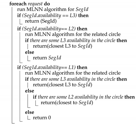
Our recommendation system considers three levels of parking place availability called L1 (zero or very low available places), L2 (several available places) and L3 (high availability) using two thresholds (i.e., T1 and T2) as follows:
less than or equal to T1 free places is considered as level L1;
between T1 and T2 free places is considered as level L2;
equal or above T2 free places is considered as level L3.
As Algorithm 1 shows, if the level of the selected parking segment by a driver is predicted as L3 for the requested time interval, the recommendation system recommends the selected segment to the driver.
If the level of the selected parking segment by a driver is predicted as L2, the system defines a circle area with center of the requested segment and radius of X (e.g., X = 500) meters. It only considers and evaluates the historical data of those parking segments that are located in the circle area. In this case, the system separately trains the best model on the data sets of each parking segment in the circle area. Finally, among the eligible parking segments (i.e., the segments in the circle area which their availability levels are L3 for the requested time interval), the closest parking segment to the requested destination is recommended to the driver. However, if the recommendation system can not find a segment with level of L3 in the circle, it offers the selected segment itself to the driver.
If the level of the selected parking segment by driver is predicted as L1, the closest L3 level parking segment to the requested destination is recommended to the driver. If there is no segment with level of L3, but there are one or more segments with L2, it suggests the closest segment with L2 to the requested segment to driver. Otherwise, the system sends a warning message to the driver.
| Algorithm 1: Segment-Selector (, timeInterval) |
![Network 02 00015 i001]() |
4. A Review on Machine Learning and Neural Network Algorithms
This section briefly introduces concept of Machine learning and Neural network, and then presents the MLNN algorithms that we study and analyze in this paper.
Primary AI research considered hard-coded statements in formal languages, which a computer according to logical inference rules can then automatically reason about (i.e., knowledge base approach). This approach has some limitations as humans generally struggle to explicate all their tacit knowledge that is needed to do complex tasks. Machine learning is utilized to overcome these limitations. It can help to make decisions by learning from previous computations and extracting regularities from large-size databases. As such, it tries to automate the task of analytical model building to do cognitive tasks such as detecting objects. It is conducted by applying MLNN algorithms that learn from problem-specific training data, which lets computers to detect hidden insights and complex patterns without explicitly being programmed. Depending on the learning task, the field offers different types of MLNN algorithms, with each algorithm coming in multiple specifications and variants, including regressions models, instance-based algorithms, decision trees, Bayesian methods, and Neural networks [
20].
In the following, we present the MLNN algorithms that we study and analyze in this paper.
4.1. K-Nearest Neighbors (KNN)
The KNN algorithm is considered as one of the simplest machine learning algorithms. It is a non-generalizing learning or lazy learning algorithm. KNN keeps all instances corresponding to training data in n-dimensional space. In order to classify a new data, it considers a simple majority vote of the k nearest neighbors of each point. In other words, every new data point is classified based on the saved data and similarity measures such as Euclidean distance function. One of the biggest challenges with KNN is to find the optimal number of neighbors. This algorithm can be utilized for both classification and regression [
21].
4.2. Decision Tree (DT) and Random Forest (RF)
DT is considered as a well-known non-parametric supervised learning method which is used for both classification and regression tasks. It constructs a tree by setting different conditions on its branches. Iterative Dichotomiser 3 (ID3), C4.5, and Classification and Regression Trees (CART) are well known for DT algorithms [
18,
21].
RF classifier is considered as an ensemble classification technique [
21]. It has been proposed in 2001 by Breiman. RF is considered as a collaborative method which works based on the proximity search. For improving the performance, RF makes use of a standard divide and conquer approach [
22]. There are a lot of similarities between the DT and RF algorithms. In fact, the RF consists of multiple independent DTs where each tree sets conditional features differently. Once a sample arrives at a root node, it is transferred to all the sub-trees where every sub-tree predicts the class label for the sample. Finally, the class in the majority is assigned to that sample [
18].
4.3. Support Vector Machines (SVMs)
For classification and clustering objectives, SVMs map data points to high dimensional vectors. If we have data points in a n-dimensional space, a (n-1)-dimensional hyperplane can be utilized as a classifier [
23].
4.4. Categorical Naive Bayes (CNB)
CNB is a relatively simple probabilistic algorithm based on the Bayes theorem. It naively assumes that the features are independent. They can be trained rather quickly using supervised learning, but are usually less accurate than more complicated approaches [
23,
24].
4.5. Single Layer Perceptron (SLP)
SLP, or simply Perceptron, is a binary classifier. It assigns a weight to every input of a Perceptron and then sums over the products of the weights and their inputs. The result is compared to a threshold in order to determine the (output) label [
23].
4.6. Multilayer Perceptron (MLP)
MLP is a Perceptron-based system that includes multiple layers: an input layer, one or more hidden layers and an output layer. By increasing the number of hidden layers, the complexity of the model increases. The MLPs can be very powerful and complex [
23,
25].
4.7. Long Short-Term Memory (LSTM)
LSTM is considered as an artificial recurrent neural network (RNN) architecture. It has been proposed to solve the vanishing and exploding gradient problems of conventional RNNs. LSTMs originally include special units called memory blocks in the recurrent hidden layer. Each memory block has a memory cell with self-connections storing the temporal state of the network and special multiplicative units (i.e., gates). An input gate is used to control the flow of input activations into the memory cell and an output gate to control the output flow of cell activations into the rest of the network [
26].
4.8. Ensemble Learning (Voting Classifier)
An ensemble learning technique combines multiple learning models in order to make a better prediction than running the algorithms separately. It takes the training data and trains each model. In the next step, it feeds the testing data to the models where each model predicts a class label for each sample in the testing data. A voting process is then performed for each sample prediction. There are two ways for voting: hard voting and soft voting. The hard voting acts based on majority where it assigns a class label, voted by majority, to the sample. The soft voting approach averages the probability of all the expected outputs (i.e., the class labels) and, after that, the class with the highest probability is assigned to the sample [
18].
5. Performance Evaluation
This section includes three main parts. We first introduce the utilized dataset and describe how we prepare and specialize it for our work. In the second part, we present technical details of our implementation including utilized tools, features, hyper-parameters, validation technique and evaluation metrics. In the third part, we first talk about our methods for implementing single algorithms, combining different algorithms (as ensemble learning) and measuring the execution time by introducing main utilized Python functions. We then define three main scenarios to evaluate single and ensemble learning algorithms as well as our proposed recommendation system.
5.1. Dataset Description
We utilized San Francisco’s dataset [
27,
28] which contains around five millions records of the measured parking availability covering a total of 420 parking segments in San Francisco. Parking availability observations were recorded at approximately 5-min intervals for each parking segment during 6 weeks.
Each line of the dataset keeps the situation of a parking segment at a specific timestamp. We consider the columns correspond to the following content:
timestamp: timestamp reporting when the SFPark API was polled, rounded to the closest minute;
segmentid: ID of the parking segment;
capacity: total number of parking places in the segment (the capacity may vary over time, due to parking restrictions);
occupied: current number of occupied places in the segment.
In addition, there is a complementary file where each line of that corresponds to a parking segment and its columns correspond to the following content:
segmentid: ID of the parking segments;
streetname: name of the related street;
startx, starty, endx, endy: WGS84 coordinates of start and end point of parking segment.
5.1.1. Data Cleaning
The obtained dataset has been already cleaned from implausible sensor values and the segments with issues have been excluded [
28]. As a result, 420 segments from the original 579 road segments have been kept and the dataset contains a total of more than 5 million observations.
In addition, we verified that:
the obtained dataset does not contain empty cells, duplicates or wrong format;
Observations are regularly and continuously recorded every 5 min for each parking segment during the considered 6 weeks.
5.1.2. Dataset Individualization
In order to provide prediction with 30 min validity, we recreated the dataset in a way that it contains availability observations at approximately 30-min intervals.
In addition, we separated the obtained dataset into 420 datasets where each new dataset contains availability observations at approximately 30-min intervals for only one individual parking segment. There are two following reasons behind this decision. First, based on the use case under study (see
Section 3), we need to predict parking place availability for a requested segment by drivers individually. In addition, for the prediction of parking availability in one special segment, we found that utilizing the whole dataset (i.e., including information of all segments together which are usually unrelated) can make a negative effect on the trained models, and therefore the results of the prediction of parking availability for that special segment. As a result, this idea could help us to reduce complexity, processing time and improve performance.
5.2. Implementation Technical Details
5.2.1. Tools and Software
The machine learning and ensemble algorithms have been implemented using Scikit-learn library [
29] and the deep learning algorithm using PyTorch [
30].
5.2.2. Input Features
According to our dataset information and the use case requirements, we define the following input features for our MLNN model:
segmentid: ID of the parking segment;
observation time: including hour and minute features which keep the hour and minute for each observation;
availability level: is calculated based on the number of free parking spots in each segment. In order to define our three availability levels, in this work, two T1 and T2 threshold values are considered equal to 3 and 10 respectively. We selected these values after doing several tests with different values. In this case:
- –
less than or equal to 3 free places is considered as level L1.
- –
between 3 and 10 free places is considered as level L2.
- –
equal or above 10 free places is considered as level L3.
streetname: name of the related street in the segment;
startx, starty, endx, endy: WGS84 coordinates of start and end point of parking segment.
5.2.3. Hyper-Parameters
In order to improve performance of the models, we found the most appropriate hyper-parameters using the Scikit-learn’s RandomSearch Cross Validation [
31]. Recall that CNB does not have hyper-parameters to tune. We considered around 16% of the dataset (i.e., one week out of 6 weeks) for tuning the hyper-parameters.
Table 1 and
Table 2 show the utilized hyper-parameter values in this work.
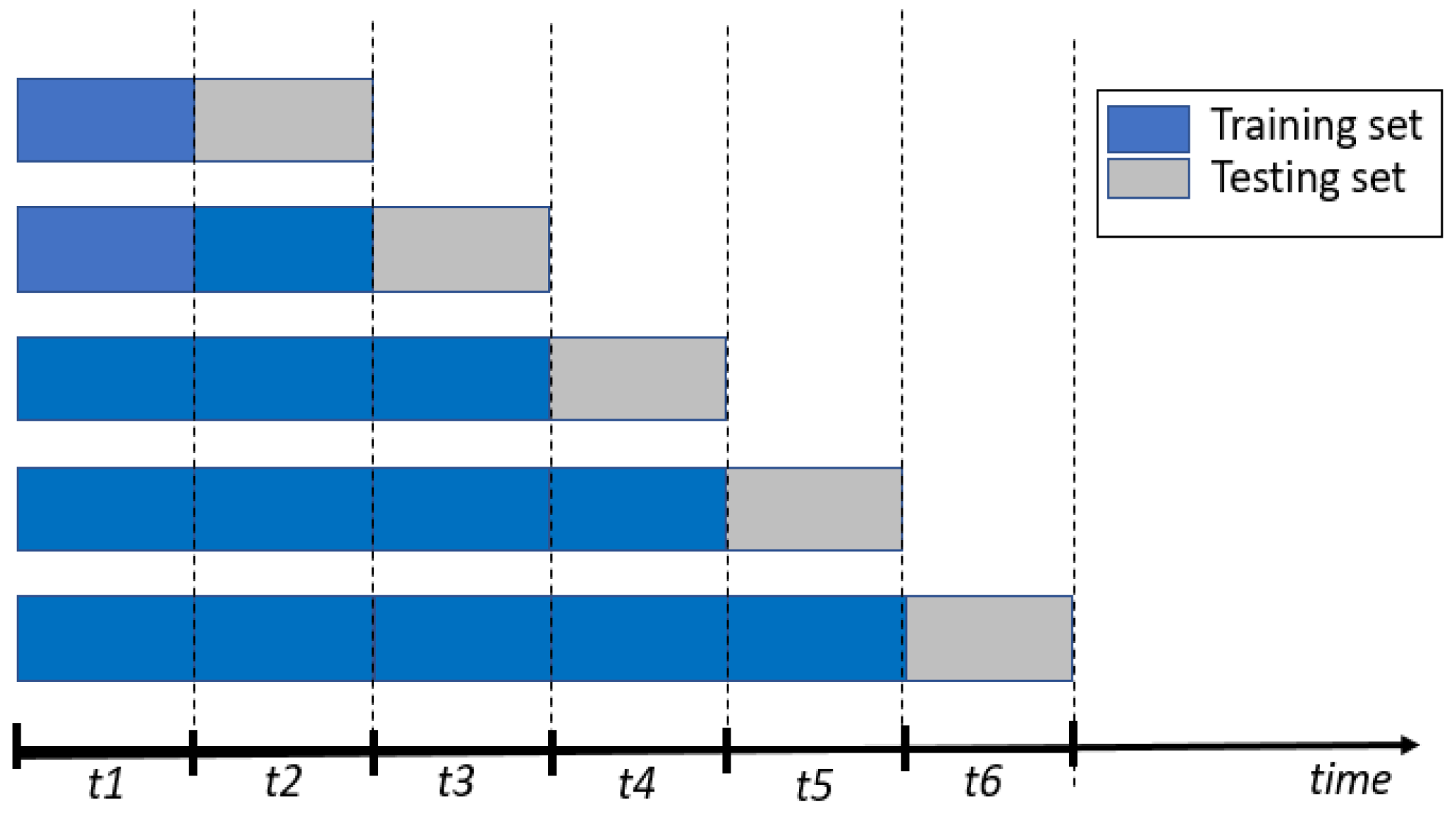
5.2.4. Validation Technique
For the time series data, using k-fold cross validation does not work perfectly. This is because it does not consider the order of data [
19].
In this work, we use a validation technique which is called walk-forward (i.e., a technique preserving the order of data).
As
Figure 1 shows, the walk-forward technique divides dataset into several units (e.g., in our work, one week as a unit). After that, units are chronologically ordered, and in each run, all data available before the unit to predict is considered as the training set, and the unit to predict is used as test-set. Finally, the model accuracy is considered as the average among runs. The number of runs is equal to one less than the number of data units [
19]. We considered around 84% of the dataset (i.e., five continues last weeks/units out of 6 weeks) for training and testing our models.
5.2.5. Evaluation Metrics
We evaluate the performance of different algorithms via Accuracy, Precision, Recall and F1 Score metrics. We also measured execution time of every algorithm (i.e., including both training and testing times).
5.3. Implementation and Evaluation
For implementing the algorithms (except LSTM), we use the Scikit-learn built-in Machine Learning classifiers (e.g., DecisionTreeClassifier for DT algorithm). For ensemble learning (i.e., combination of algorithms), we implement the hard voting technique considering the same weight for inputs (i.e., algorithms). As a result, we combine odd numbers of algorithms (i.e., 3 and 5 algorithms). To this end, we utilized the Scikit-learn voting classifier (i.e., VotingClassifier). We also use the random search function available in Scikit-learn to find appropriate values for hyper-parameters.
For calculating training/testing execution time of an algorithm, we consider the following approach. As already mentioned, we use the walk-forward technique where we need to execute every algorithm several times using different size of the dataset. We calculate an execution time by measuring the starting time and ending time of execution, and then consider the duration. To do this, we utilize the available “time” function. Finally, the execution time of an algorithm for training/testing is considered as the average of all execution times for training/testing of that algorithm.
In order to evaluate MLNN algorithms, we consider three parts. In Part.I, we implement and evaluate performance of the MLNN algorithms described in
Section 4. Notice that we use the one-vs-one method for using binary classification algorithms such as SLP for our three-class classification. Part II evaluates the performance of different combinations of MLNN algorithms, known as ensemble learning algorithms, and finally Part III implements and analyzes the proposed recommendation system introduced in
Section 3.
5.3.1. Part I-Algorithms
This part evaluates the performance of the well-known MLNN algorithms introduced in
Section 4 (i.e., KNN, DT, RF, SVM, MLP, CNB, LSTM and SLP) for predicting parking segment availability in smart cities based on accuracy, precision, recall, F1-Score and execution time.
Table 3 presents the average cross-validation score of the algorithms given 30-min predictions.
We can see that the computationally complex neural networks-based models such as LSTM, MLP and even SLP show generally the lowest performance. The results of neural networks-based models are as expected. Because generally neural networks are poor at time series forecasting. Among neural networks-based models, MLP has the best performance. It can be seen that SVM’s accuracy is the closest to the accyracy of MLP. KNN and DT, as two simple methods, show promising performance. RF can outperform other algorithms. However, it is considered as an ensemble learning method.
Table 4 compares execution time of different models (in s). Training phase for LSTM algorithm is very time consuming in comparison to other algorithms. We can see that simple algorithms such as DT and KNN have better training time than more complex ones. Considering both training and testing execution times together, DT can be considered as one of the quickest algorithms.
5.3.2. Part II-Ensemble Learning algorithms
After analyzing and comparing the performance of MLNN algorithms which are introduced in
Section 4, here, we evaluate performance of different combinations of some machine learning algorithms. The combination technique is known as Ensemble Learning or Voting Classifier. Ensemble learning combines two or more learning algorithms in order to get a better performance.
Table 5 shows results of different combination of our 7 algorithms in groups of 3 algorithms. In other words, we implemented 35 different combinations of the algorithms. As LSTM was implemented using Pytorch, due to technical limitation, we did not combine it with other algorithms. The results show that the ensemble learning methods including two neural network-based algorithms (i.e., CNB-SLP-MLP, DT-SLP-MLP, KNN-SLP-MLP, RF-SLP-MLP and SLP-SVM-MLP) have poor performance. However, as expected, a combination of a low-performance neural network algorithm with two high-performance algorithms (e.g., DT, RF and MLP) can give an acceptable performance. In general, it can be seen that there are several ensemble learning algorithms with an accuracy above 79%. Looking again at results of Part I (i.e.,
Table 4), we have only RF algorithm which its accuracy is above 79%.
According to
Table 5, a combination of DT, RF and CNB can provide the best cross validation scores (e.g., with accuracy equals to 79.81%) than other combinations.
Regarding the execution time, we can see that the combinations which contain MLP consume more time than other combinations for the training phase. It is because training phase of MLP is time consuming.
We can see, in
Table 6, results of different combination of the seven algorithms in groups of 5 algorithms. In general, the ensemble algorithms that use RF, DT and KNN together, they can provide a promising performance, especially in aspects of accuracy and recall (i.e., all above 79.5%). In particular, the results show that the combination of five KNN, DT, RF, CNB and SVM algorithms can provide the best cross validation scores (with 79.93% accuracy/recall, 81.79% precision and 79.10% f1_score) in comparison to other combinations. The second rank is the combination of KNN, DT, RF, CNB and MLP (with 79.92% accuracy/recall, 81.76% precision and 79.14% f1_score). However, because of using MLP, its training phase is time consuming.
Regarding the execution time, we can see that the combinations which contain SVM consume more time than other combinations for the training phase. It is because training of SVM is time consuming.
5.3.3. Part III-Recommendation System
The goal of this part is to evaluate the performance of the recommendation system introduced in
Section 3. In order to get an accurate result, we implemented and run Algorithm 1 ten times, and then calculated an average result. Every time, 100 drivers sent their requests. For every request, the segment number and requested time interval were selected randomly. To have more accurate results, we consider only day time (i.e., from 8:00 to 18:00). Inspiring from results of Parts I and II of this section, we used the simple but effective DT algorithm in our recommendation system. The results show that 77% of drivers selected L1 or low availability segments. It means, without using the recommendation system, 77% of drivers can not find a free spot in their selected segment and, therefore, they have to search for an available place in other segments. If we assume that finding an available place in another segment takes 5 min, for our 1000 requests, in total, the drivers should spend 1000 × 0.70 × 5 min to find a place. In this case, our recommendation system can save this time by predicting (with accuracy around 94%) selected L1 segments, and then suggesting a L3 or L2 segment.
6. Discussion
Here, we analyze and compare results of the
Table 3,
Table 4,
Table 5 and
Table 6 together. From
Table 3, we found that RF is the best algorithm (with 79.15% accuracy/recall, 80.94% precision and 78.68% f1_score) and, after RF, DT is ranked second (with 78.96% accuracy/recall, 81.09% precision and 78.64% f1_score). However, as
Table 4 shows, training phase in RF (with 0.215 s) is more time consuming than DT (with 0.0015 s). In
Table 5, we have already seen that the combination of DT, RF and CNB can provide 79.81% accuracy/recall, 81.65% precision and 79.11% f1_score with 0.2205 s training time. And, in
Table 6, we can see that the combination of five KNN, DT, RF, CNB and SVM algorithms can provide the best cross validation scores (with 79.93% accuracy/recall, 81.79% precision, 79.10% f1_score and 0.2534 s training time) in comparison to all other ensemble algorithms.
Table 7 shows the top first single algorithm (i.e., RF), the top first ensemble learning with three algorithms (i.e., DT, RF and CNB) and the top first ensemble learning with three algorithms (i.e., KNN, DT, RF, CNB and SVM). We also put DT, as a simple algorithm, to enrich our discussion. As
Table 7 shows, training time of the simple DT algorithm (i.e., 0.0015 s) is much more less than the computing-intensive ensemble algorithm with the combination of five KNN, DT, RF, CNB and SVM algorithms (i.e., 0.2534 s), while there is not a noticeable difference between performance of them (e.g., accuracy difference between them is less than 1%).
Considering the limited resources of AIoT end and even edge devices in smart parkings and also real-time nature of many AIoT applications, using simple algorithms such as DT looks more reasonable than the complex ensemble learning algorithms.
7. Conclusions
In a smart parking, AIoT can help drivers to save searching time and automotive fuel by predicting short-term parking place availability utilizing a MLNN algorithms. To find the most suitable MLNN algorithm, this paper evaluated performance of a set of well-known MLNN algorithms (i.e., KNN, DT, RF, SVM, MLP, LSTM and SLP) as well as more than 50 combinations of them (i.e., known as Ensemble Learning) based on a real parking datasets including around five millions records of the measured parking availability in San Francisco. For evaluation, we considered the cross validation scores as well as resource requirement, simplicity and execution time (i.e., including both training and testing times) of algorithms. We saw that some ensemble learning algorithms provide the best performance in aspect of validation score. However, they consume a noticeable amount of computing and time resources. On the other hand, simple algorithms such as DT and KNN could provid a much faster execution time than ensemble learning algorithms, while we could not see a noticeable difference between their performance and the best ensemble learning algorithm (e.g., DT’s accuracy is less than 1% lower than the best ensemble algorithm). In a AIoT-based smart parking, the MLNN algorithms should be run on limited-resource edge and even end device. As a result, using simple MLNN algorithms with acceptable performance such as DT can be more appropriate than complex compute-intensive ones.
We finally simulated the proposed recommendation system using the DT Algorithm. For 1000 parking spot requests from drivers, the results showed that around 77% of drivers can not find a free spot in their selected destinations (i.e., street or segment). By predicting this issue and introducing alternative closest vacant locations to destinations to the drivers, the recommended system could save, in total, 3500 min drivers searching time. Therefore, the recommendation system can help to reduce the traffic and save a noticeable amount of fuel.


